Article

Land8Fire: A Complete Study on Wildfire Segmentation Through Comprehensive Review, Human-Annotated Multispectral Dataset, and Extensive Benchmarking

1
College of Engineering, University of Arkansas, Fayetteville, AR 72701, USA
2
Center for Advanced Spatial Technologies, Fayetteville, AR 72701, USA
*
Author to whom correspondence should be addressed.
Remote Sens. 2025, 17(16), 2776; https://doi.org/10.3390/rs17162776
Submission received: 9 May 2025 / Revised: 1 July 2025 / Accepted: 12 July 2025 / Published: 11 August 2025

Abstract

Early and accurate wildfire detection is critical for minimizing environmental damage and ensuring a timely response. However, existing satellite-based wildfire datasets suffer from limitations such as coarse ground truth, poor spectral coverage, and class imbalance, which hinder progress in developing robust segmentation models. In this paper, we introduce Land8Fire, a new large-scale wildfire segmentation dataset composed of over 20,000 multispectral image patches derived from Landsat 8 and manually annotated for high-quality fire masks. Building on the ActiveFire dataset, Land8Fire improves ground truth reliability and offers predefined splits for consistent benchmarking. We evaluate a range of state-of-the-art convolutional and transformer-based models, including UNet, DeepLabV3+, SegFormer, and Mask2Former, and investigate the impact of different objective functions (cross-entropy and focal losses) and spectral band combinations (B1–B11). Our results reveal that focal loss, though effective for small object detection, underperforms in scenarios with clustered fires, leading to reduced recall. In contrast, spectral analysis highlights the critical role of short-wave infared 1 (SWIR1) and short-wave infared 2 (SWIR2) bands, with further gains observed when including near infrared (NIR) to penetrate smoke and cloud cover. Land8Fire sets a new benchmark for wildfire segmentation and provides valuable insights for advancing fire detection research in remote sensing.

1. Introduction

With climate change accelerating, the world has seen increasingly devastating wildfire seasons. Between 1999 and 2018, wildland fires burned an average of 2.8 million hectares (1 hectare ≈ 2.471 acres) per year, largely driven by extreme heat, wind, and drought [1]. In January 2025, wildfires in Palisades and Eaton scorched large areas of Los Angeles County, with economic losses estimated at USD 250 billion. Despite the efforts of thousands of firefighters, dry conditions and strong winds continue to fuel fire risk. Additionally, the August 2023 wildfires in Maui, Hawaii were among the deadliest in U.S. history, resulting in 100 fatalities and an estimated USD 5.5 billion in damages [2]. These events serve as a reminder of the devastating impacts of wildfires.
Given the increasing frequency and severity of wildfires, there is a growing need for reliable fire detection systems. Early, accurate detection and monitoring are essential to minimizing the damages caused by wildfires. However, their inherent unpredictability and tendency to ignite in remote, inaccessible areas present significant challenges to timely and effective containment. Historically, wildfire detection protocols relied on watchtowers using human observations [3]. However, dense smoke and occlusions often hindered efforts to locate the fire’s origin and track its progression. To address this, ‘point’ sensors have been used for fire detection. Point sensors are instruments that measure physical or chemical properties at a specific, localized point in space—rather than over an area or volume. These sensors activate when the surrounding air reaches a high temperature or dense smoke concentration [4]. However, they are limited in their application for early fire detection, as they are not sensitive towards onset fire temperatures. Recent efforts have aimed to address these difficulties by turning to aerial imaging for more reliable remote sensing.
A common practice involves using unmanned aerial vehicles (UAVs), or drones, due to their ability to access remote and difficult terrain. UAVs offer low operating costs and can be quickly deployed, enabling continuous monitoring and the rapid transmission of critical information for early forest fire detection [5]. However, drone- and video-based imaging can only cover small areas and often miss fires obscured by dense canopy or occlusions. Additionally, drones require trained personnel to plan and manually operate flights through forested regions. As a result, many efforts have shifted toward satellite imagery. Satellite imagery are pictures of Earth that are taken by sensors mounted on an orbiting satellite rather than by a plane, drone, or grounded camera. The satellite sensors record different properties such as how much incoming sunlight is being reflected by the ground and the thermal energy across several bands in the electromagnetic spectrum. The decreasing cost, increasing resolution, and growing availability of satellite data for the general public have made it a more favorable solution for fire detection [6].
Satellites are commonly distinguished by their spatial and temporal resolutions. Low Earth Orbit (LEO) satellites, such as Landsat-8/9 and Sentinel-2, offer high spatial resolution but have limited temporal resolution, typically revisiting the same location every few days. In contrast, Geosynchronous Equatorial Orbit (GEO) satellites, positioned much farther from Earth, provide frequent temporal coverage—capturing images of the same region multiple times per day—but at the cost of lower spatial resolution (around 2 km) [7]. One example of a GEO satellite system is the Geostationary Operational Environmental Satellites-R Series (GOES-R). However, the low spatial resolution of GOES-R limits its reliability for fire detection, with reported false alarm rates between 60% and 80% for medium- and low-confidence fire pixels [8].
The origins of satellite-based active fire (AF) detection date back to the 1960s and 1970s with airborne imaging, advancing significantly with the introduction of higher-resolution data from National Oceanic and Atmospheric Administration Advanced Very High Resolution Radiometer (NOAA’s AVHRR) sensors. These early methods relied on the sensitivity of middle infrared (MIR) spectral bands to detect thermal anomalies [9]. One of the most widely used instruments for wildfire monitoring is NASA’s Moderate Resolution Imaging Spectroradiometer (MODIS) active fire products, launched as part of the Earth Observing System [10]. MODIS provides two key capabilities: identifying the location of active fires and mapping burn scars over specified time periods [10]. The MODIS detection algorithm laid the groundwork for more advanced handcrafted AF algorithms such as VIIRS (Schroeder) [11], Murphy [12], and GOLI (Kumar and Roy) [13]. Unfortunately, thresholding methods often struggle with changing environmental factors like temperature shifts, shadows, and clouds, reducing detection accuracy [14].
In recent years, deep learning has demonstrated remarkable success in image understanding tasks, including object detection, segmentation, and classification across various domains. Convolutional neural networks (CNNs), in particular, have achieved state-of-the-art performance in applications including facial recognition, autonomous driving, and medical imaging. Moreover, deep learning methods have shown promise in remote sensing applications such as land cover and crop type classifications [15], localizing solar panels [16], waterbody mapping [17], etc. Similarly, deep learning approaches have demonstrated superior performance over traditional machine learning methods in tasks such as active fire detection, burned area mapping, and wildfire forecasting using satellite imagery [18]. Despite these advancements, remote sensing-based wildfire detection still faces several challenges including the lack of large-scale benchmark datasets with comprehensive spectral bands and accurately annotated ground truth samples [19].
To address the aforementioned challenges, we introduce the Land8Fire dataset, which builds upon the work of ActiveFire by Phiera Gha. The dataset consists of 9000 256 × 256 patches from Landsat-8 imagery, encompassing 10 spectral bands for a more comprehensive analysis of active wildfires. This dataset is built from 8194 Landsat-8 images captured globally, covering significant wildfire events since August 2020 in regions such as the Amazon, Africa, Australia, and the United States [20].
Our contributions are summarized as follows:
  • Literature Review: We present a comprehensive review of the existing wildfire segmentation methods, covering both traditional approaches and the recent advancements in deep learning.
  • Dataset: We introduce the Land8Fire dataset, a large-scale, high-resolution, human-annotated multispectral wildfire segmentation dataset designed to support the development and evaluation of wildfire detection models.
  • Benchmark: We conduct extensive benchmarking and a comprehensive comparison of various deep learning methods, which will serve as baselines for wildfire segmentation in the research domain. In addition, we investigate the impact of different loss functions and spectral band combinations to better understand their influence on model performance.
The proposed dataset and source code is publicly available on GitHub (https://github.com/UARK-AICV/Land8Fire).

2. Literature Review

2.1. Threshold-Based Wildfire Segmentation Methods

Thresholding algorithms are a fundamental image-processing technique used to classify pixels by applying a cutoff value that separates relevant features from the background [21]. In wildfire detection, these algorithms are used to isolate fire pixels by comparing their intensity values against surrounding background pixels, allowing for the identification of fire-affected areas in satellite imagery. For this research, we focus on three widely used thresholding algorithms developed specifically for Landsat-8 Operational Land Imager (OLI) data: the methods proposed by Murphy et al. [12], Schroeder et al. [22], and Kumar and Roy [13]. Murphy et al.’s algorithm, one of the first thresholding methods for Landsat-8, established a baseline by classifying fire pixels purely based on the intensity of the pixel level without considering the surrounding context. The Schroeder method improved on this by introducing a contextual approach, where thresholds are adjusted based on the values of neighboring pixels. This incorporation of spatial information is the key distinction between the two: Murphy’s method is strictly pixel-based, while Schroeder’s is context-aware. Building on both approaches, the Kumar and Roy GOLI algorithm introduced further refinements. It not only employed a variable-sized contextual window, allowing for more flexible adjustments based on local conditions, but also integrated Landsat B4 (Red) into its calculations, adding a new spectral dimension for better accuracy in specific applications.

2.1.1. Murphy et al.’s Method

In 2016, Murphy et al. [12] developed a non-contextual active fire detection algorithm for Landsat-8 OLI using thresholds based on bands 5, 6, and 7. The first step identifies unambiguous fire pixels based on the following conditions:
( ρ 7 ρ 6 1.4 ) and ( ρ 7 ρ 5 1.4 ) and ( ρ 7 0.15 )
Pixels within a 3 × 3 window around the detected fire pixels are classified as potential fire pixels. These are confirmed as fire pixels if they meet the following conditions:
( ( ρ 6 ρ 5 2 ) and ( ρ 6 0.5 ) ) or ( ( ρ 7 is saturated ) or ( ρ 6 is saturated ) )

2.1.2. Schroeder et al.’s Method

In 2016, Schroeder et al. [22] introduced a contextual approach to fire detection using Landsat-8 OLI. The algorithm applies a set of conditions that must be met for pixel classification. The first condition identifies unambiguous fire pixels:
( ( ρ 7 ρ 5 > 2.5 ) and ( ρ 7 ρ 5 > 0.3 ) and ( ρ 7 > 0.5 ) )
For highly energetic fires that may fail the initial condition, an alternative set of criteria is used:
( ( ρ 6 > 0.8 ) and ( ρ 1 < 0.2 ) and ( ρ 5 > 0.4 or ρ 7 < 0.1 ) )
The conditions in (1) are relaxed, and additional candidate fire pixels are identified using the following criteria:
( ρ 7 ρ 5 > 1.8 ) and ( ρ 7 ρ 5 > 0.17 )
Pixels identified through these relaxed conditions must pass the following contextual test to be classified as fire pixels:
( ρ 7 ρ 5 > μ ρ 7 ρ 5 + max [ 3 σ ρ 7 ρ 5 , 0.8 ] ) and ( ρ 7 > μ ρ 7 + max [ 3 σ ρ 7 , 0.08 ] ) and ( ρ 7 ρ 6 > 1.6 )
Here, μ ρ 7 ρ 5 and σ ρ 7 ρ 5 (and μ ρ 7 and σ ρ 7 ) represent the mean and standard deviation of the reflectance value in a 61 × 61 window centered around each candidate pixel, excluding water and confirmed fire pixels.

2.1.3. Kumar and Roy’s Method

In 2018, Kumar and Roy [13] further developed these methods, the GOLI algorithm, incorporating both a contextual approach and the use of Landsat-8’s band 4 (red: 0.66 μm) [13]. The first condition identifies unambiguous fire pixels based on a linear combination of reflectance values from bands 4 and 7:
ρ 4 0.53 ρ 7 0.214
Within an 8-pixel radius, additional unambiguous fire pixels are identified using the following condition:
ρ 4 0.35 ρ 6 0.044
Potential fire pixels are identified using the following conditions:
( ( ρ 4 0.53 ρ 7 0.125 ) or ( ρ 6 1.08 ρ 7 0.048 ) )
For final classification, these potential fire pixels must satisfy the following criteria, similar to Schroeder’s method:
( ρ 7 ρ 5 > μ ρ 7 ρ 5 + max ( 3 σ ρ 7 ρ 5 , 0.8 ) ) or ( ρ 7 > μ ρ 7 + max ( 3 σ ρ 7 , 0.08 ) )
Unlike Schroeder’s fixed window size, GOLI uses a variable window size r to compute the mean and standard deviation of reflectance values, further improving the contextual adaptability.

2.1.4. Thresholding Methods Strengths and Limitations

Threshold-based wildfire segmentation methods provide a simple and computationally efficient approach to fire detection, particularly effective in controlled environments. However, they face significant limitations:
  • Sensitivity to Environmental Illumination: During daylight hours, the sun’s intensity can significantly influence surface reflectance, introducing variability that may lead to false detections in remote sensing applications. This is particularly evident in channels sensitive to solar radiation. Furthermore, cloud occlusions can obscure parts of the surface, altering the intensity and distribution of light, which affects the accuracy of fire detection. Weather conditions, such as haze, fog, or varying cloud cover, can further impact the reflectance and absorption of light, introducing additional challenges in accurately detecting fire pixels.
  • Reliance on Fixed Thresholds: These methods depend on predefined thresholds for reflectance channels, making them rigid and prone to errors in dynamic environments. They often fail to adapt to varying environmental conditions, such as changes in weather or different landscapes, resulting in frequent misclassifications. As a result, highly reflective non-fire surfaces, like urban areas or deserts, are often misclassified as fire. For a detailed study on false detections in various settings, we refer readers to [20]. Furthermore, the inflexibility of these models can result in overly intense fire pixels being missed as illustrated in Figure 1 (middle).
Threshold-based wildfire segmentation methods, while straightforward and computationally efficient, face significant challenges in adapting to dynamic environments. These challenges are particularly evident when examining the performance of specific thresholding algorithms applied to diverse wildfire scenarios.
To further understand these limitations, we analyze three widely used thresholding algorithms—Schroeder et al., Murphy et al., and Kumar and Roy—focusing on their strengths and weaknesses in detecting fire pixels across different intensities and environmental conditions. As shown in Figure 1, these algorithms exhibit distinct performance patterns, particularly when detecting boundary fire regions or responding to varying fire intensities.
Upon closer inspection, while each algorithm performs well for broad fire regions, notable challenges emerge with boundary cases and specific fire characteristics. For instance, both the Murphy et al. and Kumar and Roy algorithms frequently misclassify ember flashes released from active wildfire, identifying them as part of the primary fire. This boundary misclassification is prominent in the middle and bottom rows of Figure 1, where scattered embers surrounding the fire’s edge are often marked as active fire pixels (shown in blue). False positives can compromise accuracy, particularly when embers are near but not part of the main fire.
Further analysis reveals that the Kumar and Roy algorithm, although effective at identifying clustered fire pixels, struggles when faced with detecting smaller, isolated fire pixels. These tiny pixels, particularly those outside larger clusters, tend to go undetected, leading to instances of under-segmentation in less intense fire areas. This limitation suggests that while effective for prominent clusters, the algorithm may not be optimal for sparse or dispersed fire activity, which is critical in early detection scenarios.
Another challenge observed across all thresholding algorithms is their difficulty in detecting intense wildfire pixels as shown in the middle rows of Figure 1. Highly saturated or overexcited pixels often fall outside the algorithms’ fixed threshold ranges, leading to frequent misclassifications or complete omissions. These high-intensity regions exhibit significant variability in pixel values, which static thresholding methods struggle to handle. While approaches such as adaptive thresholding or incorporating additional spectral bands can improve sensitivity and granularity in these cases, calibrating thresholds continues to be a complex and delicate task. Adjusting the threshold to better capture intense pixels can inadvertently affect other parts of the detection process, leading to either missed detections in less intense regions or an increase in false positives around the fire’s boundaries. This limitation underscores the complex trade-offs involved in threshold selection, where enhancing sensitivity in one area can compromise accuracy in another, especially when working with highly variable wildfire data.
Overall, while thresholding algorithms are effective at identifying primary fire regions, they fall short in more complex scenarios—such as detecting fire boundaries, isolated fire pixels, and saturated regions. These limitations highlight the need for more adaptive solutions. In response, recent research has increasingly turned to machine learning methods to improve wildfire segmentation performance.

2.2. Machine Learning-Based Wildfire Segmentation Methods

Machine learning (ML) algorithms have been widely applied to wildfire detection and segmentation, offering varying degrees of success based on the techniques used. These methods can be broadly categorized into two groups: conventional ML-based methods and deep learning (DL)-based methods.

2.2.1. Conventional ML-Based Methods

Conventional machine learning methods learn directly from data, allowing them to detect wildfires without needing expert-defined rules or precise modeling of complex environmental variables, such as fuel composition or weather patterns. Traditional ML methods are often interpretable and suitable for smaller datasets with well-defined features [23]. Milanović et al. used logistic regression (LR) and random forest (RF) to map forest fire probability in Eastern Serbia, finding that RF models outperformed LR in predictive ability, with drought code as the most important variable for fire occurrence [24]. Molovtsev et al. evaluated the performance of various machine learning models on a dataset of forest fires in the Russian Federation, concluding that RF exhibited high performance, while decision tree, LR, and support vector machine (SVM) models performed poorly in early fire detection [25]. Hong et al. compared the performance of RF and SVM for fire detection, concluding that RF outperforms SVM in overall performance. While SVM identifies most points as fire, leading to low accuracy and recall, RF achieves better recall but still faces issues with low precision and more false positives, indicating room for improvement in accuracy and false alarm rates [26]. While machine learning models like RF and SVM show potential for wildfire detection, their effectiveness is often constrained by the specifics of the dataset and the geographical region being analyzed. The type of wildfire, whether severe or mild, as well as the terrain play significant roles in determining model performance [27]. This makes these methods highly inflexible when applied across different regions and varying wildfire conditions. As a result, a model that performs well in one area may not generalize effectively to other regions or different types of fire events, limiting their broader applicability for wildfire occurrences across diverse landscapes. These limitations have motivated the development of deep learning-based solutions. Therefore, our work will focus exclusively on deep learning-based methods for wildfire segmentation, omitting traditional machine learning approaches in our experiments due to their limited scalability and adaptability.

2.2.2. Deep Learning-Based Methods

In recent years, DL-based fire segmentation has gained prominence for its ability to address the inherent limitations of threshold-based approaches and conventional ML approach. Unlike conventional ML, which often relies on handcrafted features, DL automatically extracts and learns hierarchical features from raw data. Within fire segmentation, it involves grouping similar pixels of smoke or flame in satellite images according to their characteristics, such as color, shape, and texture, and producing a corresponding mask as output [18]. Reis et al. (2023) evaluated the UNet architecture for fire hotspot detection using Sentinel-2 images [28]. Akbari et al. (2023) evaluated a variety of UNet structures: UNet with stochastic ReLU activation, UNet with dropout layers, and probabilistic UNet, which integrates U-Net with a conditional variational auto-encoder [29]. Seyd et al. (2022) developed Fire-Net, using a two-stream deep learning approach: one stream focusing on identifying fire pixels and the other on detecting background elements [14]. Additionally, this architecture uses multi-scale residual convolution layers, enabling the model to handle different fire sizes by processing features at multiple scales, which improves the detection for both large and small fires [14].
DL-based methods show great promise in automatically detecting wildfires, offering advantages in feature extraction and segmentation performance. However, there are several limitations: (i) these methods are often evaluated on small datasets, which can lead to overfitting, as deep learning models typically require vast amounts of training data to generalize effectively; and (ii) many existing methods are benchmarked against ground-truth data created using threshold-based methods, meaning that DL-based approaches are inherently constrained by the performance of those algorithmic methods. To overcome these challenges, it is essential to create large-scale, high-quality datasets with standardized benchmarking to fully realize the potential of deep learning in wildfire detection.

2.3. Wildfire Datasets

One critical factor in the reliability of aerial imaging for wildfire detection is the availability and quality of datasets. For instance, the FLAME and predecessor FLAME2 dataset, consists of unmanned aerial vehicle (UAV) data, capturing fire videos and images during prescribed burning slash piles [30,31]. However, UAVs still require human involvement and face limitations in flight duration and distance, making them less suitable for long-term wildfire surveillance [32].
The California Department of Forestry and Fire Protection’s Fire and Resource Assessment Program (FRAP) maintains an annual wildfire perimeter dataset for California, developed with input from federal and state agencies. While comprehensive, it has limitations due to missing or incomplete data, including unrecorded small fires and over-generalizations in some perimeters [33]. Similarly, the Pyregence open-source fire science platform integrates various datasets for real-time fire spread models, including static inputs like fuel and topography, weather forecasts and real-time fire progression data, providing valuable tools for fire prediction and analysis [34]. While datasets that map burned areas are crucial for assessing post-fire recovery and rehabilitation, they lack real-time imagery, making them less useful for monitoring active fires. These datasets do not provide RGB or multispectral scene representations, limiting their ability to capture fires in progress. For active fire datasets, we study the following datasets: Sen2Fire [35] and ActiveFire [20].
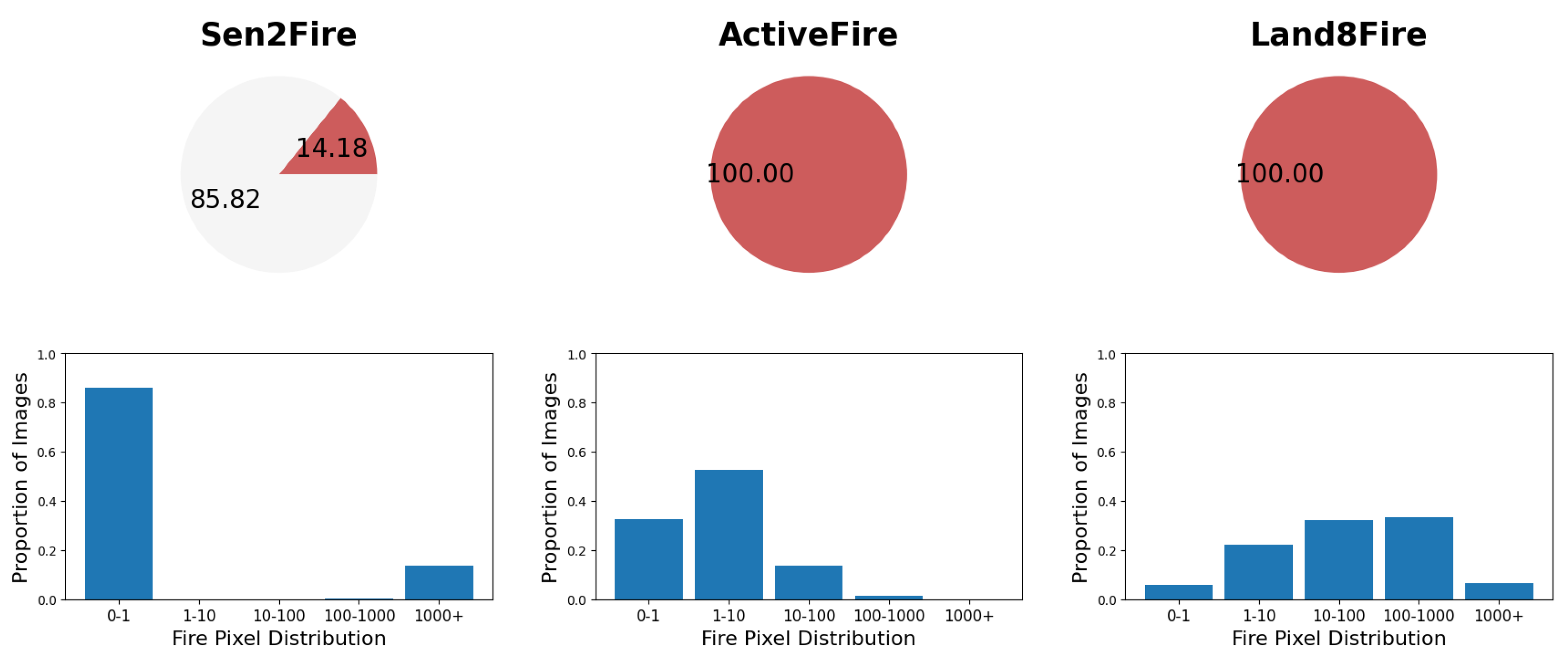
Sen2Fire [35] provides a satellite-based fire segmentation dataset derived from Sentinel-2 multispectral data and Sentinel-5P aerosol products. It consists of 2466 image patches (512 × 512 with 128-pixel overlap) across 13 spectral bands. The ground truth labels are generated using the MOD14AI V6.1 product, with a spatial resolution of 1 km. Additionally, Sen2Fire exhibits a highly imbalanced distribution of fire pixels. Figure 2 (top row) shows that only 14.18% of images contain fire pixels, while the remaining majority have no fire present. Furthermore, Figure 2 (bottom row) highlights the dataset’s skewed fire pixel distribution, where most images contain either very few fire pixels (<1) or an extremely high number (>1000), with no intermediate cases. This imbalance poses challenges for segmentation models, as it may lead to biases favoring non-fire regions.
Similarly, ActiveFire [20] is a large-scale dataset containing over 150,000 image patches (256 × 256 without overlap) extracted from Landsat-8 images, covering 10 spectral bands across all continents except Antarctica. Similarly, its ground truth is derived from automated threshold-based algorithms, raising concerns regarding segmentation accuracy. Additionally, our analysis shows that every image in the ActiveFire dataset contains at least one fire pixel. However, it remains unclear whether this was an intentional design choice. This raises concerns about potential false positives, as the ground truth is generated using an algorithm that inherently introduces classification errors. As a result, it is likely that the approximately 30% of the dataset falling within the [0–1] fire pixel distribution range in Figure 2 (bottom row)—implying these images contain exactly one fire pixel—is due to misclassification by the algorithm.
Despite notable contributions from existing wildfire datasets, there remains a significant gap in resources that seamlessly integrate high-resolution and long duration fire tracking. After evaluating the two datasets, Sen2Fire and ActiveFire both provide a good basis for wildfire detection, each having distinct strengths and weaknesses. As shown in Table 1, Sen2Fire offers a variety of spectral bands. However, it suffers from a small sample size, with only four wildfire occurrences studied. Additionally, its ground truth is generated using a thresholding algorithm, making its accuracy uncertain. On the other hand, ActiveFire is a much larger dataset, covering a wide variety of wildfire occurrences, including a variety of spectral bands. Additionally, like Sen2Fire, its ground truth data are derived from thresholding algorithms, introducing similar concerns regarding accuracy.

3. Land8Fire Dataset Curation

The Land8Fire dataset addresses the limitations in existing wildfire datasets by providing a large-scale collection with 10 spectral bands, and most importantly manually validated masks to improve ground truth accuracy. The dataset originates from the ActiveFire subset of full-sized Landsat 8 images. For details on the initial dataset, refer to Pereira et al. [20]. The original dataset contained 76 images, each accompanied by masks generated using the Schroeder (2016) conditions. From this set, we selected all images with more than 950 fire pixels (19 images)—an arbitrarily chosen threshold based on human observation. Additionally, we randomly selected 7 more images from the remaining 57, each containing fewer than 950 fire pixels. The Schroeder-generated masks and their corresponding visual representations (SWIR2, SWIR1, and Blue bands) were loaded into an annotation tool, Computer Vision Annotation Tool (CVAT) for manual validation. This band combination was chosen because it provides an enhanced version of traditional RGB imagery; the SWIR2, SWIR1, and Blue bands produce more saturated colors that help visually distinguish fire pixels from the background with greater clarity. To maintain consistency, all annotations were performed by a single annotator. We verified our annotation through spot checks using alternative spectral bands with the other two thresholding-based methods. Additionally, we re-annotated a small batch after several weeks to assess consistency over time. Although this process significantly improves label quality, small fire pixels remain susceptible to human annotation error.
Rather than cropping the full-sized images, which could result in many patches without fire pixels, we focused on isolating wildfire groupings. For each grouping, we drew bounding rectangles and cropped 256 × 256 patches within these boundaries, applying a 220-pixel overlap. This overlap was chosen to ensure that the fire features near patch edges were preserved. Without overlap, important contextual information may be lost, particularly near patch borders where CNN-based models often struggle. Although this simple overlap strategy introduces some spatial redundancy, it effectively captures edge regions more completely in at least one patch. This approach yielded over 20,000 image patches, each containing 10 spectral bands. The full curation process, from manual annotation to bounding box selection and patch extraction, is illustrated in Figure 3. Landsat 8 provides 11 spectral bands, but our dataset excludes Band 8 (panchromatic, 0.500–0.680 μ) due to its higher resolution (15 m) compared to the other bands, which have a 30 m resolution (Table 2).
Rather than prioritizing geographic or seasonal diversity, Land8Fire emphasizes fire pixel imbalance by curating a diverse range of wildfire types—clustered, scattered, and small-scale fires—to better reflect the challenges of fine-grained fire detection.

4. Experiments

4.1. Evaluation Metrics

To assess model performance in fire segmentation, we compute five key metrics—mean accuracy (mAccuracy), precision, recall, intersection over union (IoU), and F1-score—focusing solely on the fire class. Given the dataset’s imbalance, we prioritize metrics that effectively balance fire pixel detection and misclassification. All metrics derive from the four basic values: true positive (TP), true negative (TN), false positive (FP) and false negative (FN).
mAccuracy measures the average proportion of correctly classified pixels across all images, accounting for both fire and non-fire pixels. It is defined as
mAccuracy = 1 n i = 1 n T P i + T N i T P i + T N i + F P i + F N i
While mAccuracy provides a broad performance assessment, it can be misleading in imbalanced datasets, where a model may achieve high accuracy simply by classifying most pixels as non-fire.
Precision quantifies the proportion of predicted fire pixels that are true fire:
Precision = T P f i r e T P f i r e + F P f i r e
A high precision score indicates the model effectively minimizes false positives, which is critical for reducing false alarms. False positives in wildfire detection can lead to unnecessary resource allocation, public distress, and inefficient emergency responses [36]. However, optimizing for precision alone can cause the model to miss actual fire pixels.
Recall, also known as sensitivity, evaluates the model’s ability to detect actual fire pixels:
Recall = T P f i r e T P f i r e + F N f i r e
High recall ensures that fewer fire pixels are misclassified as non-fire, minimizing false negatives. Since missing fire pixels can have severe consequences, including delayed wildfire response, recall is crucial for accurate fire detection [37]. By emphasizing true positives, recall ensures that all potential fire occurrences, even sparse ones, are detected.
Intersection over Union (IoU), also known as the Jaccard Index, assesses the spatial overlap between the predicted and actual fire pixels:
IoU = T P f i r e T P f i r e + F P f i r e + F N f i r e
IoU is particularly valuable for segmentation tasks, as it penalizes both false positives and false negatives. A high IoU score indicates that the predicted fire regions closely align with the ground truth, making it a robust metric for evaluating model effectiveness in imbalanced datasets [38].
F1-score, the harmonic mean of precision and recall, provides a balanced assessment of a model’s ability to detect fire pixels while minimizing misclassification:
F 1 - Score = 2 × T P f i r e 2 × T P f i r e + F P f i r e + F N f i r e

4.2. Evaluation Metric Analysis

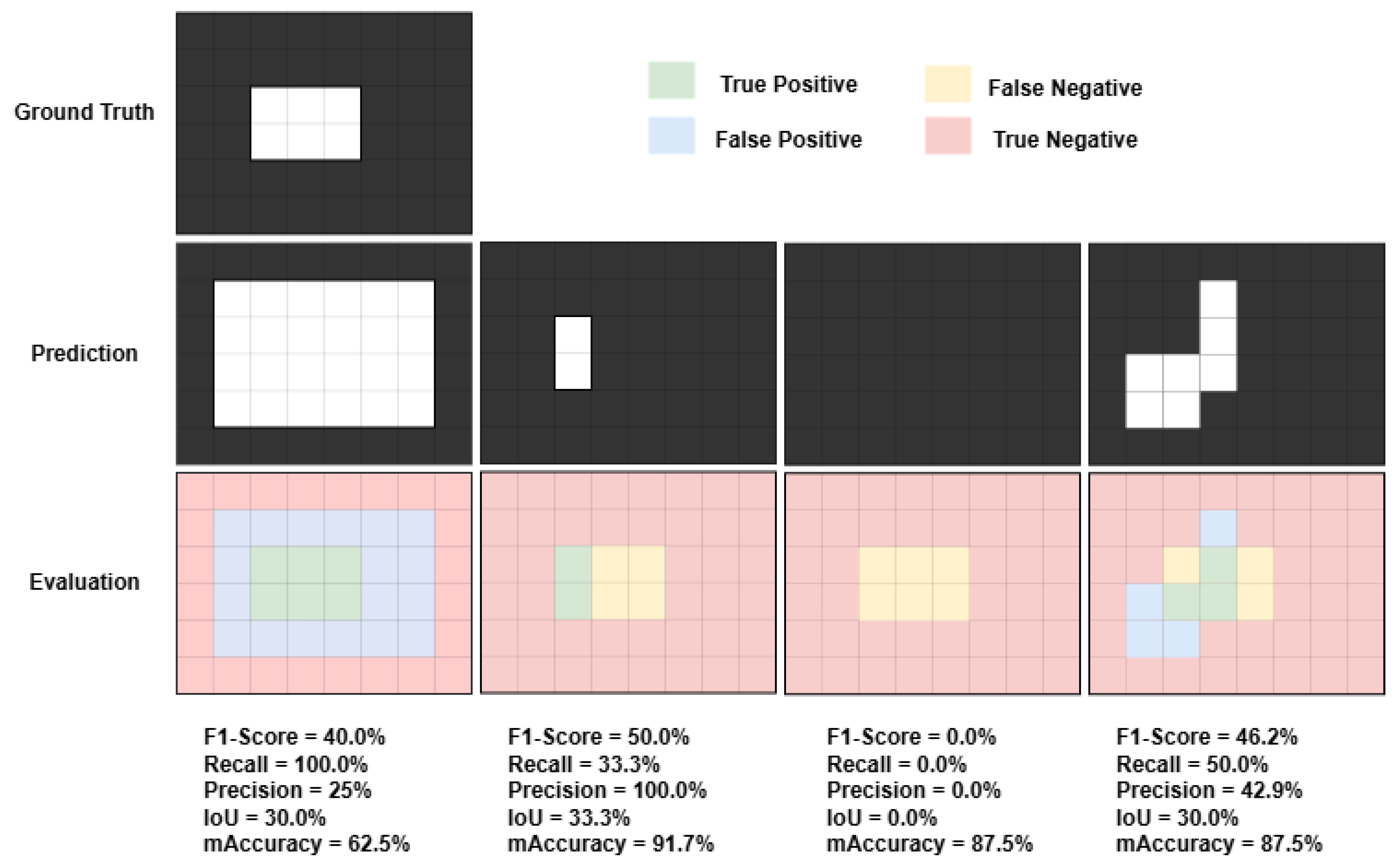
While these metrics provide quantitative definitions, understanding their practical implications requires visual context. To illustrate how different prediction scenarios impact each metric, we analyze segmentation outputs in Figure 4, highlighting the trade-offs between precision, recall, IoU, F1-score, and mAccuracy in different scenarios.
Figure 4 demonstrates the conceptual difference between the F1-score, recall, precision, mAccuracy, and IoU in the context of fire pixel segmentation. The ground truth mask (top-center) serves as the reference. The overpredicted mask (left) extends beyond the actual fire region, capturing all ground truth fire pixels while introducing false positives. As a result, it achieves a perfect recall (100.0%) but low precision (25.0%). Conversely, the underpredicted mask (top right) identifies only a subset of actual fire pixels. This leads to a perfect precision (100.0%), since all the predicted fire pixels are correct, but low recall (33.3%), as many fire pixels are missed. This visual illustrates how precision and recall must be balanced in wildfire detection tasks to ensure reliable and actionable segmentation results. Because recall and precision often conflict, the F1-score provides a more balanced metric by considering both. In the overpredicted and underpredicted mask in Figure 4, the F1-score is 40.0% and 50.0%, respectively, demonstrating the balance between recall and precision. In the context of wildfire detection, where missing a fire or misclassifying non-fire regions can both have serious consequences, we adopt F1-score as our primary evaluation metric, using precision and recall to further analyze model behavior. The third example (bottom-left) is an extreme case where the model fails to predict any fire pixels, i.e., predicting everything as the background. In this case, F1-score, recall, precision, and IoU are 0%, yet the mAccuracy remains 87.5%. This is because the model correctly identifies most background pixels (true negatives), which dominate the image. This example highlights a key weakness of mean accuracy in class-imbalanced scenarios like wildfire detection, where it can appear deceptively high even when the model completely fails to detect any fire present. In the final example (bottom-right), the model produces a noisy prediction containing both false positives and false negatives. Recall (50%) and precision (42.9%) are moderate, while IoU is 30%, matching the IoU seen in the overpredicted example. However, despite these predictions having identical IoU values, the underlying error types are completely different: one misses many true fire pixels, while the other overpredicts fire regions. This demonstrates a key limitation of IoU—it reflects the degree of spatial overlap but fails to distinguish how the model failed. In contrast, the F1-score (46.2%) captures the balance between false positives and false negatives, offering a clearer and more informative view of the model’s behavior.
By focusing on these class-specific metrics, we provide a robust evaluation of the model’s ability to detect fire pixels accurately while mitigating the effects of dataset imbalance. This ensures our segmentation model not only identifies fire regions effectively but also minimizes false alarms and missed detections.

4.3. Deep Learning Architecture Analysis

To assess model performance in fire segmentation, we use several deep learning architectures that have been briefly mentioned above: CNNs such as FCN, U-Net, PSPNet, UPerNet, and DeepLabV3+, and Transformers such as Mask2Former and SegFormer. Each of these models is well-documented through extensive online resources and open-source implementations, providing robust frameworks for addressing the challenges of fire segmentation in remote sensing imagery.

4.3.1. CNN-Based Segmentation Models

  • Fully Convolutional Networks (FCNs)
FCNs, introduced by Long et al. [39], were the first models designed to perform semantic segmentation using deep learning. FCNs adapt traditional CNNs by replacing the final fully connected layers with convolutional layers, allowing the network to make spatially aware, per-pixel predictions instead of assigning a single label to the entire image.
FCNs extract hierarchical features using convolution and pooling, then apply upsampling (using transpose convolutions) to restore the spatial resolution of the original input. This makes FCNs effective at identifying large regions of interest in an image. However, FCNs struggle to recover fine details, especially along object boundaries or with small and scattered targets, making them less effective in tasks requiring high spatial precision, such as early-stage wildfire detection.
2.
UNet
UNet, introduced by Ronneberger et al. [40], was originally developed for biomedical image segmentation but has since become a popular model for remote sensing and wildfire detection tasks. It follows an encoder–decoder structure that balances both high-level abstraction and precise localization.
The encoder is a standard CNN that uses repeated convolution and pooling layers to reduce the spatial resolution while increasing the depth of feature maps, capturing the contextual (semantic) features of the input. The decoder gradually upsamples the features using transpose convolutions to reconstruct the original spatial resolution. What makes UNet especially effective is its use of skip connections—these directly transfer feature maps from the encoder to the decoder at corresponding levels. This helps the model retain fine-grained spatial information that would otherwise be lost during downsampling.
Skip connections are essential for preserving small details such as edges or tiny fire pixels. As the encoder downsamples the input image through convolution and pooling, some fine details—like edges or small objects—can become lost. Skip connections solve this by directly copying the feature maps from the encoder and merging them with the corresponding decoder layers. By merging encoder features with decoder layers, the model obtains both global context and local detail. As a result, UNet’s ability to localize small targets makes it effective in detecting early-stage fires.
3.
Pyramid Scene Parsing Network (PSPNet)
PSPNet, introduced by Zhao et al. [41], was designed to enhance semantic segmentation by capturing both local and global context. Unlike traditional CNN-based architectures that struggle to model global scene understanding, PSPNet introduces a pyramid pooling module (PPM) to address this limitation.
The encoder of PSPNet is built on top of a deep residual network (e.g., ResNet), which extracts hierarchical feature maps from the input image. After the encoder, instead of directly feeding the final feature map into a decoder, PSPNet inserts a pyramid pooling module. This module performs pooling at multiple spatial scales to aggregate contextual information from different regions of the image. These pooled features are then upsampled and concatenated with the original feature map, creating a rich representation that captures both fine and coarse details across the image. This combined feature map is then passed through a final convolution layer to generate the pixel-wise segmentation output.
PSPNet excels in scenarios where context is crucial, such as distinguishing between similarly colored objects based on their surroundings. For wildfire detection, its multi-scale feature aggregation helps differentiate between fire and background in complex natural scenes. However, due to its reliance on global pooling, it may struggle with precisely locating small or scattered fire pixels—unlike models like UNet that use skip connections to retain spatial detail.
4.
Unified Perceptual Parsing Network (UPerNet)
UPerNet, introduced by Xiao et al. [42], was designed to improve semantic segmentation by integrating multi-scale features across different network stages. While traditional CNN-based segmentation models often focus only on deep high-level features, UPerNet enhances segmentation by combining both low-level spatial detail and high-level semantic context.
The encoder of UPerNet is typically a pre-trained backbone like ResNet, which extracts hierarchical features from different stages of the network. Instead of relying on just the final layer, UPerNet taps into multiple feature stages—similar to a Feature Pyramid Network (FPN). These intermediate features capture varying levels of semantic abstraction and spatial resolution.
To aggregate the global context, UPerNet incorporates a pyramid pooling module (PPM)—borrowed from PSPNet—into the final encoder output. This module performs pooling at multiple scales to gather rich global context. These pooled features are upsampled and fused with the original high-level feature before being passed into the decoder.
The decoder then merges the outputs from different encoder stages using top–down fusion, progressively upsampling and combining lower-stage features (which have finer resolution) with higher-stage features (which contain more abstract information). This structure allows UPerNet to simultaneously capture fine-grained spatial detail and broad contextual understanding.
UPerNet is especially useful in segmentation tasks involving complex scenes where both the local and global information matter—like wildfire imagery that includes smoke, fire, trees, and terrain. Its multi-level fusion and pyramid pooling make it more flexible than basic FCNs or PSPNet alone. However, its complexity and reliance on fusion steps may make it less efficient for detecting very small and isolated fire pixels.
5.
DeepLabV3+
DeepLabV3+, introduced by Chen et al. [43], is an advanced semantic segmentation model that builds upon the DeepLab series by combining Atrous Spatial Pyramid Pooling (ASPP) with an encoder–decoder structure.
The encoder uses a deep CNN backbone (ResNet) to extract high-level semantic features from the input image. To expand the receptive field and capture multi-scale information, it applies dilated convolutions allowing the network to extract features from wider contexts without downsampling the image. At the core of this process is the ASPP module, which applies parallel dilated convolutions at multiple rates to gather rich contextual information across various spatial scales. The decoder then upsamples the feature maps using transpose convolutions and fuses them with low-level features from earlier encoder layers. This fusion helps recover spatial details lost during encoding and ensures that fine boundaries, such as those around fire edges, are preserved in the final segmentation mask.
Unlike UNet, DeepLabV3+ does not rely on symmetric skip connections at each level. Instead, it selectively merges low-level encoder features with the upsampled high-level ASPP output in a lightweight decoder. This design balances efficiency with accuracy, making it especially effective for segmenting larger or more complex wildfire regions—though it may underperform on very small, sparse fires.

4.3.2. Transformer-Based Segmentation Models

  • Mask2Former
Mask2Former, introduced by Cheng et al. [44], is a unified transformer-based framework for semantic, instance, and panoptic segmentation. It builds on the earlier MaskFormer design by replacing convolutional backbones with a fully transformer-driven architecture for both feature extraction and segmentation refinement.
In MaskFormer, features are first extracted using a backbone like ResNet and then passed through a pixel-level decoder such as ASPP (from DeepLabV3+) or PPM (from PSPNet). These refined features are then fed into a transformer decoder, which predicts and iteratively refines segmentation masks. The key innovation in Mask2Former is its masked attention mechanism. Rather than applying self-attention across the entire image, the model focuses only on relevant regions defined by the current predicted masks. This lets it refine predictions with high spatial precision, attending only to areas that matter.
Mask2Former excels in complex segmentation tasks requiring the precise delineation of object boundaries and fine-grained scene understanding. In the context of wildfire detection, its attention-based refinement can help separate active fire regions from surrounding noise such as smoke or clouds. However, due to its complexity and reliance on large amounts of high-quality training data, it may underperform in detecting small or early-stage fires.
2.
SegFormer
SegFormer, introduced by Xie et al. [45], is a lightweight and efficient transformer-based model designed for semantic segmentation. It was created to combine the representational power of transformers with the efficiency and simplicity often associated with CNN-based models, making it highly suitable for resource-constrained environments like real-time segmentation or edge devices.
SegFormer uses a hierarchical encoder called the MixVision Transformer (MiT), which processes images in multiple stages. Early layers capture fine spatial detail, while deeper layers extract high-level semantic features—forming a pyramid-like architecture similar to FPN but that is entirely transformer-based. Unlike traditional transformers that use positional encodings, SegFormer adopts overlapping patch embeddings using convolutions with stride smaller than kernel size. This preserves the local continuity and spatial structure without the need for explicit position information. The extracted features are then passed to a simple multi-layer perceptron (MLP) decoder, which fuses multi-scale features and produces the final segmentation map—avoiding heavier modules like ASPP or PPM.
SegFormer is both fast and accurate, making it suitable for real-time or edge applications. In wildfire detection, it performs well in a large-scale context but may miss very small fire pixels due to its lack of explicit mask refinement.

4.4. κ -Fold Cross-Validation

To ensure robust evaluation and mitigate the risk of overfitting due to the limited size of the Land8Fire dataset, we employ κ -fold cross-validation as our validation strategy. κ -fold cross-validation is a widely used resampling technique in machine learning, particularly beneficial for small datasets, as it allows models to be trained and evaluated on multiple data splits rather than relying on a single partition of the dataset [46,47]. This method enhances the reliability of model performance estimates by reducing variability across different data splits.
In κ -fold cross-validation, the dataset is divided into κ equal-sized subsets (folds). The model is trained on ( κ − 1) folds and tested on the remaining fold. This process is repeated κ times, with each fold serving as the test set once, and the final model performance is computed as the average of all κ iterations [48]. For this study, we used 5-fold cross-validation ( κ = 5), meaning the dataset is split into five parts, and each model is trained and evaluated five times. We report the mean performance across all five folds for accuracy, IoU, recall, precision, and F1-score, ensuring a comprehensive and statistically reliable assessment of each segmentation model in Table 3.
To avoid spatial leakage caused by overlapping patches from the same geographic region, we did not use a purely random fold assignment. Instead, we partitioned the dataset by grouping patches based on their Landsat-8 scene identifiers (LCO8_…_RT_{cluster identifier}_{counter}), where each identifier corresponds to a distinct fire event or spatial cluster. Patches from a single cluster were assigned exclusively to one fold, ensuring that no spatially correlated data appeared in both training and test sets.
To balance fire pixel distribution across folds, we first recorded the number of patches in each cluster and then randomly shuffled the cluster groups. Using a rolling counter, we assigned clusters to each fold until reaching approximately one-fifth of the total dataset for the first four folds, with the remaining clusters assigned to the fifth. We did not reserve a separate test set; instead, in each run, four folds were used for training and the remaining fold for testing.

4.5. Implementation Details

The experiments were conducted on single-GPU with a Quadro RTX 8000 GPU (48 GB). The implementation was performed using MMSegmentation, an open-source semantic segmentation toolbox based on the Pytorch library. We trained each architecture using the Adam optimizer with a learning rate of 0.0001 and a batch size of 32, and ran the training for 25,000 iterations.

4.6. Wildfire Detection Results

In this experiment, we benchmarked two categories of wildfire segmentation methods: (i) threshold-based methods, including Schroeder [22], Kumar and Roy [13], and Murphy [12], and (ii) deep learning-based methods, including FCN [39], UNet [40], PSPNet [41], DeepLabV3+ [43], Mask2Former [44], and SegFormer [45] as presented in Table 3. For all deep learning-based models, we employed the commonly used cross-entropy (CE) loss to optimize pixel-level classification. CE loss measures how well the model distinguishes between fire and background pixels by comparing each predicted class with its corresponding ground truth label. This pixel-wise formulation encourages the network to assign higher confidence to correct predictions and penalizes misclassifications accordingly. Under this loss function, the deep learning models are trained using the following objective:
L o s s C E = i = 1 n t i log ( p i ) , where p i = 1 1 + e x
where t i represents the ground truth, and p i is the softmax probability for the i t h class. In the binary segmentation setting, these probabilities are obtained using the sigmoid function, ensuring proper probability distribution across fire and non-fire pixels. This loss function serves as a baseline, enabling a later comparison with more specialized loss functions, such as focal loss, to address class imbalance more effectively. This comparison aims to evaluate the role of the loss function in balancing precision and recall, especially for fire pixel detection.
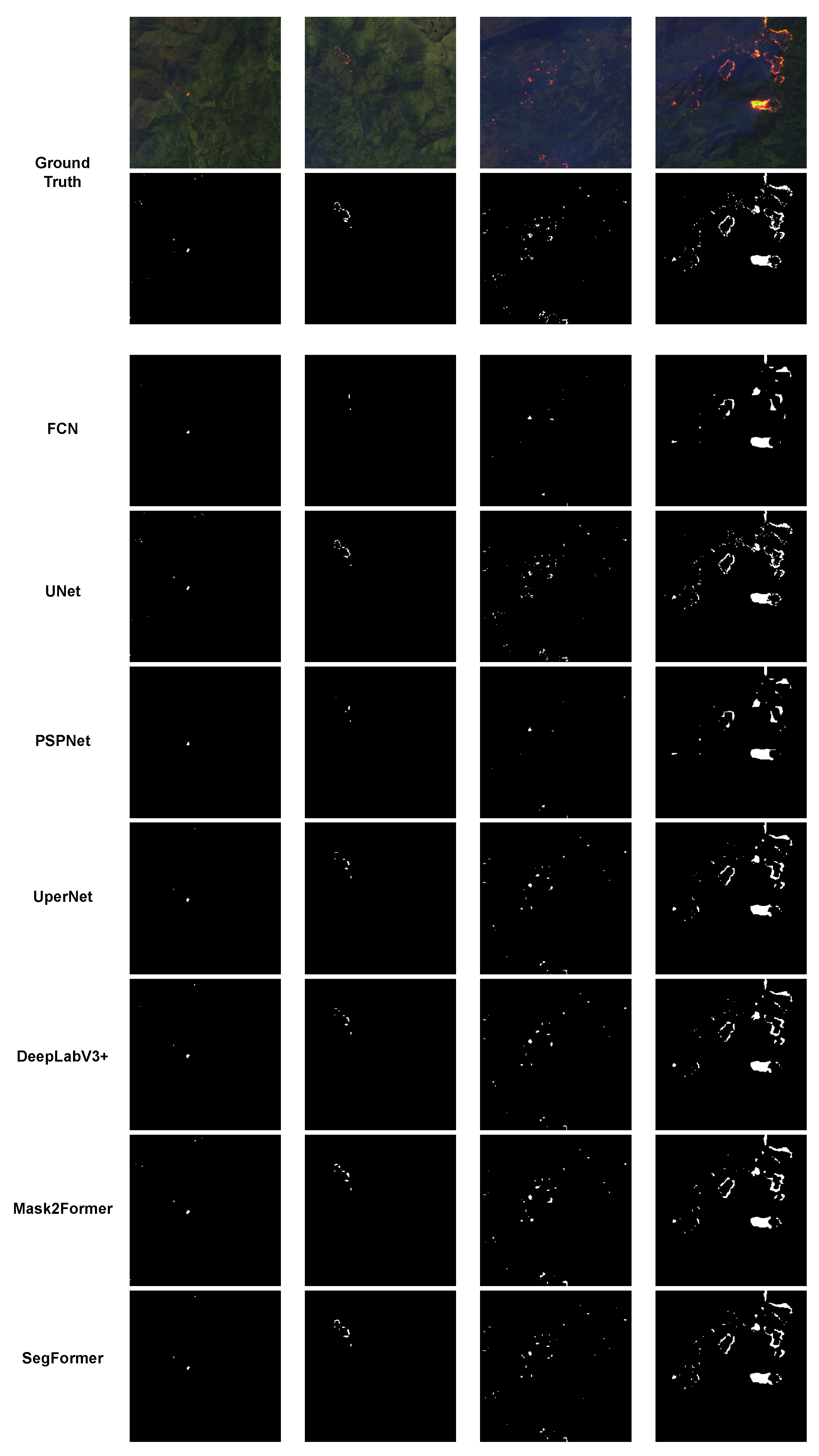
As shown in Table 3, the performance of deep learning-based segmentation models varies significantly on the Land8Fire dataset, with UNet demonstrating the strongest results across all metrics. UNet achieves an F1-score of 94.49%, along with a recall of 93.28%, precision of 95.76%, overall accuracy of 91.49%, and an IoU of 89.58%, outperforming all other models in the benchmark. UNet is the most effective model for wildfire detection, with its high F1-score emphasizing a strong balance between precision and recall. Figure 5 further illustrates the superior segmentation capability of UNet across various fire scenarios, particularly in small early-stage fires and scattered fire occurrences, where other models struggle with misclassification.
Other models, such as UPerNet, Mask2Former, SegFormer, and DeepLabV3+, also deliver competitive results, with F1-scores near 80%. Their respective recalls range from 74.42% to 77.20%, and precision values are consistently high, ranging from 82.54% to 83.90%. These models also achieve solid overall accuracies between 87.17% and 88.56%, and IoUs in the 65.35% to 67.36% range, indicating good segmentation performance, though not matching the level of accuracy of UNet. The higher precision but low recall suggests that while they maintain reliability, they might under-detect smaller fire regions, leading to missed detections in cases where fire is more dispersed.
Similarly, the threshold-based methods, such as those of Schroeder, Kumar and Roy, and Murphy, demonstrate competitive results with F1-scores of 87.58%, 70.75%, and 74.25%, respectively, but fail to achieve competitive segmentation quality compared to UNet. These methods rely on predefined thresholding rules, which lead to high precision (99.76%) but lower recall (82.98%) as seen in Schroeder’s algorithm, or vice versa as seen in those of Kumar and Roy, and Murphy, which have high recall (91.96% and 98.62%) but poor precision (61.08% and 62.44%). This imbalance indicates that thresholding methods either over-detect fire pixels, leading to high false positives, or under-detect them, missing smaller fire occurrences.
In contrast, FCN and PSPNet show significantly lower segmentation performance. Both models yield F1-scores of 64.99% and 64.77%, with recalls of 55.77% and 55.34%, precision of 79.54% and 80.38%, overall accuracies of 77.85% and 77.64%, and IoUs just under 50%. These results suggest that FCN and PSPNet struggle to capture fine-grained fire regions effectively, making them less suitable for wildfire segmentation in remote sensing imagery.

4.7. Discussion

Despite being state-of-the-art architectures, transformer-based models like Mask2Former and SegFormer underperform compared to UNet. These models typically require large, task-specific datasets to fully realize their potential. Although our dataset includes approximately 22,000 patches (with ≈18,000 used for training), this may still be insufficient for effective transformer learning. In addition, transformers often require more careful tuning, including longer training schedules and optimized learning rate strategies. However, to ensure a fair and consistent comparison across all models, we maintained the same training setup, including a 25,000 iteration limit, for each architecture, which may not be enough for transformers to fully converge. That said, the standard deviation for these models are moderate, suggesting a degree of stability despite their underperformance.
As expected, UPerNet and DeepLabV3+ also underperform relative to UNet in our wildfire segmentation task. Both models are designed to capture global context and parse complex scene structures, often at the expense of fine-grained spatial precision. This trade-off makes them less effective at detecting small, sparse fire regions, where accurate boundary delineation is crucial. Like the transformer-based models, UPerNet and DeepLabV3+ exhibit moderate standard deviation across evaluation folds, reflecting some sensitivity to data variation but not to the extent of older architectures.
On the other hand, PSPNet and FCN—being older and less specialized—struggle to resolve fine edges and small fire pixels, resulting in both lower performance and higher standard deviation across all metrics. This indicates greater instability and poor generalization across folds. Their limited ability to model fine-grained spatial features, along with outdated architectural designs, likely contribute to this inconsistency.
In contrast, the strong inductive biases of UNet, particularly spatial locality, make it better suited for learning from limited data and smaller training time. Furthermore, its consistently low standard deviation further highlights its ability to generalize under such constraints and can be attributed to its superior performance on Land8Fire.

4.8. Abalation Study: Objective Function

In addition to traditional cross-entropy (CE) loss, we conduct an ablation study to evaluate the effectiveness of focal loss in addressing the class imbalance present in our dataset. As illustrated in Figure 2, the Land8Fire dataset exhibits a severe imbalance between fire and non-fire pixels. In most cases, fire pixels constitute a very small fraction of the total image. Specifically, approximately 90% of Land8Fire images contain fewer than or equal to 1000 fire pixels. Given that each image patch is 256 × 256 pixels (totaling 65,536 pixels), this means fire pixels often make up only around 1.5% of the image. This imbalance significantly increases the risk of the model becoming biased toward predicting the dominant background class. Given this distribution, it becomes necessary to evaluate how well deep learning models can handle imbalanced data, especially in the context of early-stage fire detection, where small fires may appear as just a few pixels.
To address this, we compare focal loss against CE loss in our experiments. Originally proposed by Lin et al. [49], focal loss mitigates class imbalance by down-weighting easy examples, allowing the model to focus on hard-to-classify pixels:
L o s s F o c a l = i = 1 n ( i p i ) γ log ( p i )
It dynamically scales the CE loss, removing the need for explicit resampling while still encouraging attention to minority classes. This is especially relevant in wildfire segmentation, where small fires often appear as sparse or isolated pixels. Fires in their initial stages may span only a few pixels, making them difficult to detect using conventional loss functions biased toward majority classes. By emphasizing harder examples during training, focal loss improves the model’s sensitivity to these small underrepresented fire regions, making it a strong candidate for unbalanced pixel-wise segmentation tasks like this.
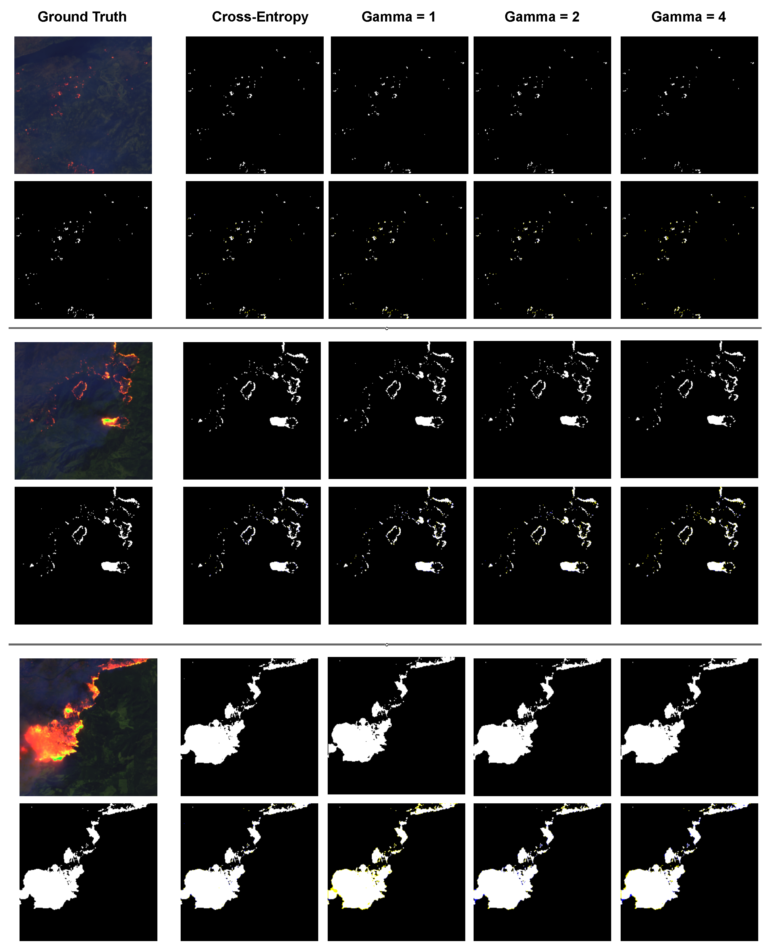
To assess the effectiveness of focal loss in wildfire segmentation, we applied focal loss with varying gamma values to a UNet model and compared its performance against traditional CE loss. As shown in Table 4, the results indicate that UNet with focal loss performs worse across all evaluation metrics compared to CE.
While focal loss is highly effective for small object detection, its failure in our wildfire segmentation task highlights an important distinction. Focal loss is best suited for detecting small, isolated objects, such as single-pixel or tiny fire instances scattered across an image. However, the Land8Fire dataset features not only sparse fire pixels but also extensive clustered fire regions, which presents a different challenge. As illustrated in Figure 6, focal loss tends to struggle with these larger fire clusters, resulting in higher false negative rates, even in areas where fires are visually prominent. This occurs because the loss function overemphasizes rare, ambiguous fire pixels and underweights confident predictions, thereby reducing the model’s ability to fully segment well-defined fire regions. The result is a noticeable drop in recall, as the model misses substantial portions of clustered fires. Instead of improving segmentation performance, focal loss suppresses predictions for larger, more easily detectable fire areas, ultimately harming the overall detection capability. While focal loss is designed to handle extreme class imbalance, it is not well-suited for wildfire segmentation where fires often appear in clusters rather than as isolated small objects.

4.9. Band Analysis

Unlike traditional image classification tasks that primarily use Red, Green, Blue (RGB) inputs, wildfire detection benefits significantly from multispectral imaging. Since aerial imagery captures active wildfires from above, smoke and cloud cover can obscure flames, making detection in standard RGB channels unreliable.
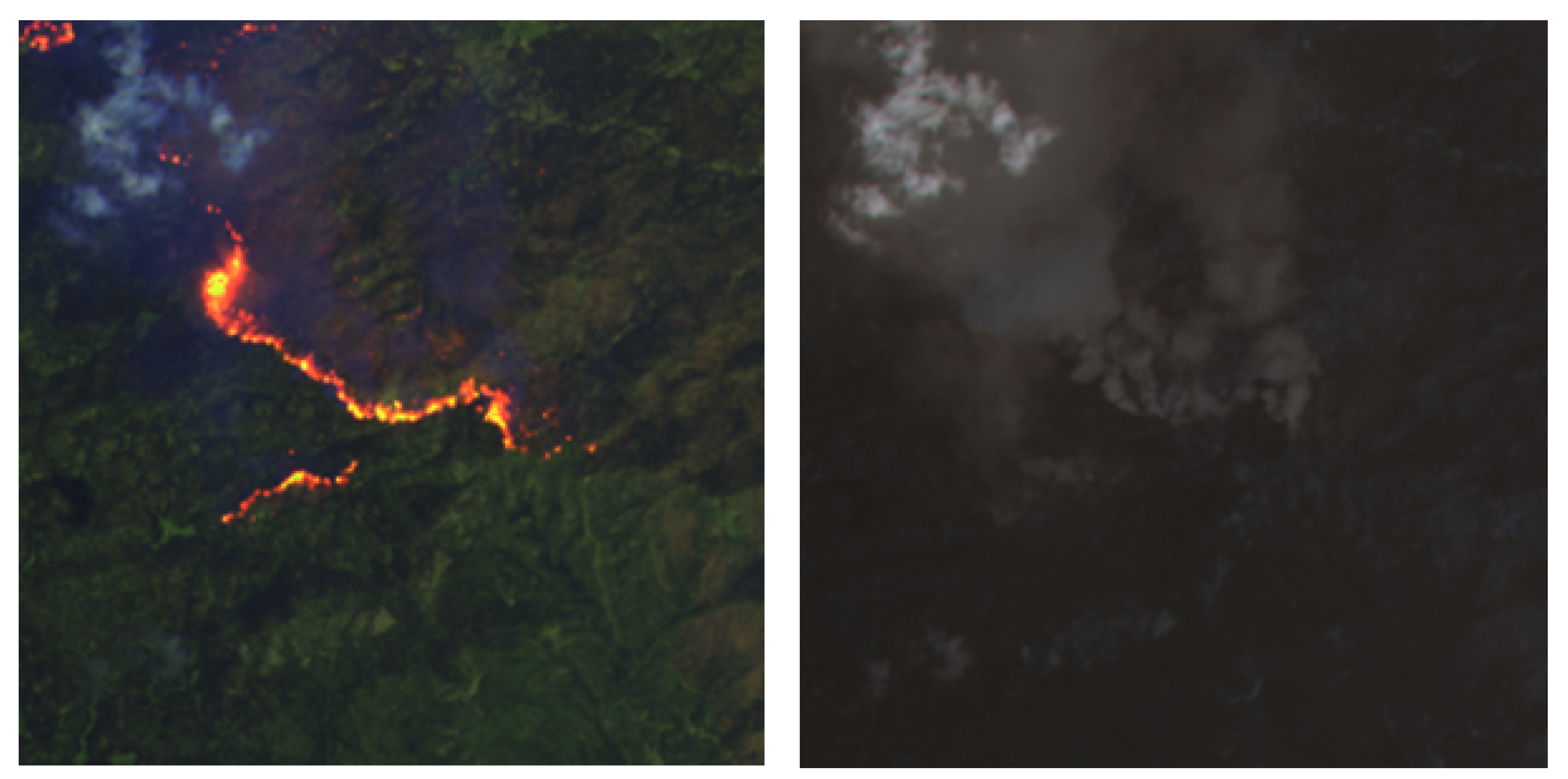
Figure 7 illustrates this challenge by comparing a visual representation of short-wave infrared bands (B2 (Blue) + B6 (SWIR1) + B7 (SWIR2)) (left) with a raw visible Landsat image (right) using standard (B4 (Red) + B3 (Green) + B2 (Blue)) (RGB) channels. The SWIR-based visualization enhances thermal anomalies, making active fire regions more distinguishable, whereas the RGB image often fails to highlight fire pixels clearly.
Given the importance of spectral band selection, a key question arises: which band combinations optimize wildfire segmentation performance? While prior studies have identified B6 (SWIR1) and B7 (SWIR2) as critical for fire detection, alternative band selections have been used in various threshold-based algorithms. For example, Schroeder [22] uses bands 1, 5, 6, and 7; Kumar and Roy [13] use bands 5, 6, and 7; and Murphy [12] uses bands 4, 5, 6, and 7. To systematically evaluate the impact of different spectral inputs, we trained UNet on the Land8Fire dataset using multiple band configurations, as summarized in Table 5.
As shown in Table 5, the combination B5+B6+B7 (NIR + SWIR1 + SWIR2) produced the best results, achieving an F1-score of 96.99%, recall of 97.24%, precision of 96.73%, mAccuracy of 98.61%, and IoU of 94.15%. These results confirm that adding near infrared alongside the short wave infrared bands significantly boosts the model’s ability to accurately isolate fire pixels. Similarly, the combination B4+B5+B6+B7 (Red + NIR + SWIR1 + SWIR2) also performed well, with an F1-score of 96.39%, suggesting that including the Red band may help, but it does not provide as much benefit as NIR and SWIR do. These findings align with the prior research [50], which emphasizes that SWIR wavelengths are particularly sensitive to thermal anomalies—making them ideal for fire detection, especially when smoke or cloud occlusions are present.
In contrast, setups limited to just the visible bands—specifically B2 + B3 + B4 (Blue, Green, Red)—performed the worst. This configuration resulted in an F1-score of 32.70% and an IoU of just 19.55%, clearly showing that visible light alone is not enough to reliably distinguish fire from the background in satellite imagery.
Interestingly, using all available bands (B1–B7, B9–B11) did not lead to the best results either. Although the full-band configuration achieved a strong F1-score of 96.17%, it still underperformed compared to more selective combinations like B5 + B6 + B7. This suggests that not all bands contribute meaningful information—some may even introduce redundancy or spectral noise, ultimately degrading the segmentation performance. This is consistent with the findings from [50], which suggest that while bands B1 to B5 often capture smoke or haze, they fail to reliably isolate the fire core, especially when used without complementary thermal bands.
Although our original use of the blue band (B2) helped with creating visually interpretable representations of the scene, this choice did not translate into strong segmentation performance. B2 lacks the spectral distinction needed to robustly differentiate fire from background, particularly when smoke is present. With this analysis, it becomes clear that training with SWIR1, SWIR2, and NIR is a better choice. Overall, this highlights that optical band selection is a critical step in designing reliable wildfire segmentation when using deep learning models, as they are sensitive to the quality of input features.

5. Conclusions

In this paper, we introduce Land8Fire, a large-scale and high-resolution wildfire segmentation dataset designed to advance research in remote sensing-based fire detection. Land8Fire contains over 20,000 image patches with manually validated ground truth masks, providing a more reliable and challenging benchmark for semantic segmentation.
The value of Land8Fire extends beyond model benchmarking. It provides a robust and realistic testing ground for evaluating the generalizability of segmentation methods in real-world wildfire scenarios, particularly those involving wide variations in fire size and intensity. From sparse, low-intensity ignitions to dense, high-intensity fire clusters, the dataset captures the full spectrum of wildfire behavior. We benchmark a range of state-of-the-art deep learning methods including both CNN-based and transformer-based, offering new insights into their performance on real-world wildfire imagery. Beyond model evaluation, we investigate the impact of different loss functions and various spectral band selections.
Our findings show that despite focal loss helping in retrieving small fire pixels, it is less effective in clustered fire scenarios in general compared to the CE loss. Additionally, spectral analysis revealed that B5 (NIR), B6 (SWIR1), and B7 (SWIR2) bands are the most critical for effective fire detection, especially under cloud or smoke occlusion.
Future work shall focus on investigating alternative loss functions, such as Tversky loss, Dice loss, and class-balanced focal loss, which may offer better performance in handling imbalanced datasets and improving segmentation accuracy, particularly for small or scattered fire regions.
We hope that Land8Fire can serve as a foundation for future research in fine-grained wildfire segmentation and contribute to the development of more accurate and reliable fire detection systems in remote sensing.

Author Contributions

Conceptualization, A.T., M.T. and E.M.; formal analysis, J.C. and N.L.; methodology, A.T., M.T. and E.M.; project administration, J.C. and N.L.; validation, A.T., M.T. and E.M.; writing-review and editing, A.T., E.M., J.C., C.R., S.E. and N.L. All authors have read and agreed to the published version of the manuscript.

Funding

This research was funded by Student Undergraduate Research Fellowship (SURF), University of Arkansas Honors College Research Grant, National Science Foundation (NSF) under Award No OIA-1946391 RII Track-1, NSF 2345176.

Data Availability Statement

In this study, we compared three datasets: Sen2Fire, ActiveFire, and Land8Fire. The Sen2Fire is available at https://zenodo.org/records/10881058. The ActiveFire dataset is publicly available at https://github.com/pereira-gha/activefire. Lastly, the Land8Fire dataset can be acessed at https://github.com/UARK-AICV/Land8Fire. Please refer to the provided links for futher details.

Conflicts of Interest

The authors declare no conflicts of interest.

References

  1. Jaffe, D.A.; O’Neill, S.M.; Larkin, N.K.; Holder, A.L.; Peterson, D.L.; Halofsky, J.E.; Rappold, A.G. Wildfire and prescribed burning impacts on air quality in the United States. J. Air Waste Manag. Assoc. 2020, 70, 583–615. [Google Scholar] [CrossRef] [PubMed]
  2. NOAA National Centers for Environmental Information. Billion-Dollar Weather and Climate Disasters: Summary Statistics; Technical Report; NOAA National Centers for Environmental Information: Asheville, NC, USA, 2024.
  3. Dampage, U.; Bandaranayake, L.; Wanasinghe, R.; Kottahachchi, K.; Jayasanka, B. Forest fire detection system using wireless sensor networks and machine learning. Sci. Rep. 2022, 12, 46. [Google Scholar] [CrossRef]
  4. Huang, P.; Chen, M.; Chen, K.; Zhang, H.; Yu, L.; Liu, C. A combined real-time intelligent fire detection and forecasting approach through cameras based on computer vision method. Process Saf. Environ. Prot. 2022, 164, 629–638. [Google Scholar] [CrossRef]
  5. Khan, A.; Hassan, B.; Khan, S.; Ahmed, R.; Abuassba, A. DeepFire: A Novel Dataset and Deep Transfer Learning Benchmark for Forest Fire Detection. Mob. Inf. Syst. 2022, 2022, 5358359. [Google Scholar] [CrossRef]
  6. Upadhyay, P.; Gupta, S. Introduction To Satellite Imaging Technology And Creating Images Using Raw Data Obtained From Landsat Satellite. ICGTI-2012 2012, 1, 126–134. [Google Scholar]
  7. Koltunov, A.; Ustin, S.L.; Prins, E.M. On timeliness and accuracy of wildfire detection by the GOES WF-ABBA algorithm over California during the 2006 fire season. Remote Sens. Environ. 2012, 127, 194–209. [Google Scholar] [CrossRef]
  8. Badhan, M.; Shamsaei, K.; Ebrahimian, H.; Bebis, G.; Lareau, N.P.; Rowell, E. Deep Learning Approach to Improve Spatial Resolution of GOES-17 Wildfire Boundaries using VIIRS Satellite Data. Remote Sens. 2024, 16, 715. [Google Scholar] [CrossRef]
  9. Wooster, M.J.; Roberts, G.J.; Giglio, L.; Roy, D.P.; Freeborn, P.H.; Boschetti, L.; Justice, C.; Ichoku, C.; Schroeder, W.; Davies, D.; et al. Satellite remote sensing of active fires: History and current status, applications and future requirements. Remote Sens. Environ. 2021, 267, 112694. [Google Scholar] [CrossRef]
  10. Justice, C.; Giglio, L.; Korontzi, S.; Owens, J.; Morisette, J.; Roy, D.; Descloitres, J.; Alleaume, S.; Petitcolin, F.; Kaufman, Y. The MODIS fire products. Remote Sens. Environ. 2002, 83, 244–262. [Google Scholar] [CrossRef]
  11. Schroeder, W.; Oliva, P.; Giglio, L.; Csiszar, I.A. The New VIIRS 375 m active fire detection data product: Algorithm description and initial assessment. Remote Sens. Environ. 2014, 143, 85–96. [Google Scholar] [CrossRef]
  12. Murphy, S.W.; de Souza Filho, C.R.; Wright, R.; Sabatino, G.; Pabon, R.C. HOTMAP: Global hot target detection at moderate spatial resolution. Remote Sens. Environ. 2016, 177, 78–88. [Google Scholar] [CrossRef]
  13. Kumar, S.S.; Roy, D.P. Global operational land imager Landsat-8 reflectance-based active fire detection algorithm. Int. J. Digit. Earth 2018, 11, 154–178. [Google Scholar] [CrossRef]
  14. Seydi, S.T.; Saeidi, V.; Kalantar, B.; Ueda, N.; Halin, A.A. Fire-Net: A Deep Learning Framework for Active Forest Fire Detection. J. Sens. 2022, 2022, 8044390. [Google Scholar] [CrossRef]
  15. Kussul, N.; Lavreniuk, M.; Skakun, S.; Shelestov, A. Deep learning classification of land cover and crop types using remote sensing data. IEEE Geosci. Remote Sens. Lett. 2017, 14, 778–782. [Google Scholar] [CrossRef]
  16. De Luis, A.; Tran, M.; Hanyu, T.; Tran, A.; Haitao, L.; McCann, R.; Mantooth, A.; Huang, Y.; Le, N. SolarFormer: Multi-scale transformer for solar PV profiling. In Proceedings of the 2024 International Conference on Smart Grid Synchronized Measurements and Analytics (SGSMA), Washington, DC, USA, 21–23 May 2024; pp. 1–8. [Google Scholar]
  17. Chen, Y.; Fan, R.; Yang, X.; Wang, J.; Latif, A. Extraction of urban water bodies from high-resolution remote-sensing imagery using deep learning. Water 2018, 10, 585. [Google Scholar] [CrossRef]
  18. Ghali, R.; Akhloufi, M.A. Deep learning approaches for wildland fires using satellite remote sensing data: Detection, mapping, and prediction. Fire 2023, 6, 192. [Google Scholar] [CrossRef]
  19. Rashkovetsky, D.; Mauracher, F.; Langer, M.; Schmitt, M. Wildfire detection from multisensor satellite imagery using deep semantic segmentation. IEEE J. Sel. Top. Appl. Earth Obs. Remote Sens. 2021, 14, 7001–7016. [Google Scholar] [CrossRef]
  20. de Almeida Pereira, G.H.; Fusioka, A.M.; Nassu, B.T.; Minetto, R. Active fire detection in Landsat-8 imagery: A large-scale dataset and a deep-learning study. ISPRS J. Photogramm. Remote Sens. 2021, 178, 171–186. [Google Scholar] [CrossRef]
  21. Bhargavi, K.; Jyothi, S. A survey on threshold based segmentation technique in image processing. Int. J. Innov. Res. Dev. 2014, 3, 234–239. [Google Scholar]
  22. Schroeder, W.; Oliva, P.; Giglio, L.; Quayle, B.; Lorenz, E.; Morelli, F. Active fire detection using Landsat-8/OLI data. Remote Sens. Environ. 2016, 185, 210–220. [Google Scholar] [CrossRef]
  23. Janiesch, C.; Zschech, P.; Heinrich, K. Machine learning and deep learning. Electron. Mark. 2021, 31, 685–695. [Google Scholar] [CrossRef]
  24. Milanović, S.; Marković, N.; Pamučar, D.; Gigović, L.; Kostić, P.; Milanović, S.D. Forest fire probability mapping in eastern Serbia: Logistic regression versus random forest method. Forests 2020, 12, 5. [Google Scholar] [CrossRef]
  25. Molovtsev, M.D.; Sineva, I.S. Classification algorithms analysis in the forest fire detection problem. In Proceedings of the 2019 International Conference “Quality Management, Transport and Information Security, Information Technologies” (IT&QM&IS), Sochi, Russia, 23–27 September 2019; pp. 548–553. [Google Scholar]
  26. Hong, Z.; Tang, Z.; Pan, H.; Zhang, Y.; Zheng, Z.; Zhou, R.; Ma, Z.; Zhang, Y.; Han, Y.; Wang, J.; et al. Active fire detection using a novel convolutional neural network based on Himawari-8 satellite images. Front. Environ. Sci. 2022, 10, 794028. [Google Scholar] [CrossRef]
  27. Collins, L.; McCarthy, G.; Mellor, A.; Newell, G.; Smith, L. Training data requirements for fire severity mapping using Landsat imagery and random forest. Remote Sens. Environ. 2020, 245, 111839. [Google Scholar] [CrossRef]
  28. Reis, C.E.P.; dos Santos, L.B.R.; Morelli, F.; Vijaykumar, N.L. Deep Learning-Based Active Fire Detection Using Satellite Imagery. In Proceedings of the International Conference on Intelligent Systems Design and Applications, Olten, Switzerland, 11–13 December 2023; pp. 148–157. [Google Scholar]
  29. Akbari Asanjan, A.; Memarzadeh, M.; Lott, P.A.; Rieffel, E.; Grabbe, S. Probabilistic wildfire segmentation using supervised deep generative model from satellite imagery. Remote Sens. 2023, 15, 2718. [Google Scholar] [CrossRef]
  30. Shamsoshoara, A.; Afghah, F.; Razi, A.; Zheng, L.; Fulé, P.Z.; Blasch, E. Aerial imagery pile burn detection using deep learning: The FLAME dataset. Comput. Netw. 2021, 193, 108001. [Google Scholar] [CrossRef]
  31. Chen, X.; Hopkins, B.; Wang, H.; O’Neill, L.; Afghah, F.; Razi, A.; Fulé, P.; Coen, J.; Rowell, E.; Watts, A. Wildland fire detection and monitoring using a drone-collected rgb/ir image dataset. IEEE Access 2022, 10, 121301–121317. [Google Scholar] [CrossRef]
  32. Mohapatra, A.; Trinh, T. Early wildfire detection technologies in practice—A review. Sustainability 2022, 14, 12270. [Google Scholar] [CrossRef]
  33. California Department of Forestry and Fire Protection (CAL FIRE). CAL FIRE Data Portal. 2025. Available online: https://data.ca.gov/group/fire (accessed on 7 March 2025).
  34. Saah, D. Open Science in Wildfire Risk Management: Bridging the Gap with Innovations from Pyregence, Climate and Wildfire Institute, RiskFactor, Delos, and Planscape. In Proceedings of the AGU Fall Meeting Abstracts, San Francisco, CA, USA, 11–15 December 2023; Volume 2023, p. NH32A-03. [Google Scholar]
  35. Xu, Y.; Berg, A.; Haglund, L. Sen2Fire: A Challenging Benchmark Dataset for Wildfire Detection using Sentinel Data. arXiv 2024, arXiv:2403.17884. [Google Scholar] [CrossRef]
  36. Davis, J.; Goadrich, M. The relationship between Precision-Recall and ROC curves. In Proceedings of the 23rd International Conference on Machine Learning, Pittsburgh, PA, USA, 25–29 June 2006; pp. 233–240. [Google Scholar]
  37. Sokolova, M.; Lapalme, G. A systematic analysis of performance measures for classification tasks. Inf. Process. Manag. 2009, 45, 427–437. [Google Scholar] [CrossRef]
  38. Rahman, M.A.; Wang, Y. Optimizing intersection-over-union in deep neural networks for image segmentation. In Proceedings of the International Symposium on Visual Computing, Las Vegas, NV, USA, 12–14 December 2016; pp. 234–244. [Google Scholar]
  39. Long, J.; Shelhamer, E.; Darrell, T. Fully convolutional networks for semantic segmentation. In Proceedings of the IEEE Conference on Computer Vision and Pattern Recognition, Boston, MA, USA, 7–12 June 2015; pp. 3431–3440. [Google Scholar]
  40. Ronneberger, O.; Fischer, P.; Brox, T. U-net: Convolutional networks for biomedical image segmentation. In Proceedings of the Medical Image Computing and Computer-Assisted Intervention—MICCAI 2015: 18th International Conference, Munich, Germany, 5–9 October 2015; pp. 234–241. [Google Scholar]
  41. Zhao, H.; Shi, J.; Qi, X.; Wang, X.; Jia, J. Pyramid scene parsing network. In Proceedings of the IEEE Conference on Computer Vision and Pattern Recognition, Honolulu, HI, USA, 21–26 July 2017; pp. 2881–2890. [Google Scholar]
  42. Xiao, T.; Liu, Y.; Zhou, B.; Jiang, Y.; Sun, J. Unified perceptual parsing for scene understanding. In Proceedings of the European Conference on Computer Vision (ECCV), Munich, Germany, 8–14 September 2018; pp. 418–434. [Google Scholar]
  43. Chen, L.C.; Zhu, Y.; Papandreou, G.; Schroff, F.; Adam, H. Encoder-decoder with atrous separable convolution for semantic image segmentation. In Proceedings of the European Conference on Computer Vision (ECCV), Munich, Germany, 8–14 September 2018; pp. 801–818. [Google Scholar]
  44. Cheng, B.; Misra, I.; Schwing, A.G.; Kirillov, A.; Girdhar, R. Masked-attention mask transformer for universal image segmentation. In Proceedings of the IEEE/CVF Conference on Computer Vision and Pattern Recognition, New Orleans, LA, USA, 18–24 June 2022; pp. 1290–1299. [Google Scholar]
  45. Xie, E.; Wang, W.; Yu, Z.; Anandkumar, A.; Alvarez, J.M.; Luo, P. SegFormer: Simple and efficient design for semantic segmentation with transformers. Adv. Neural Inf. Process. Syst. 2021, 34, 12077–12090. [Google Scholar]
  46. Arlot, S.; Celisse, A. A survey of cross-validation procedures for model selection. Statist. Surv. 2010, 4, 40–79. [Google Scholar] [CrossRef]
  47. Kohavi, R. A study of cross-validation and bootstrap for accuracy estimation and model selection. Ijcai 1995, 14, 1137–1145. [Google Scholar]
  48. Manual, A.B. An introduction to Statistical Learning with Applications in R; Springer: New York, NY, USA, 2013. [Google Scholar]
  49. Lin, T.Y.; Goyal, P.; Girshick, R.; He, K.; Dollár, P. Focal loss for dense object detection. In Proceedings of the IEEE International Conference on Computer Vision, Venice, Italy, 22–29 October 2017; pp. 2980–2988. [Google Scholar]
  50. Singh, H.; Ang, L.M.; Srivastava, S.K. Active wildfire detection via satellite imagery and machine learning: An empirical investigation of Australian wildfires. Nat. Hazards 2025, 121, 9777–9800. [Google Scholar] [CrossRef]
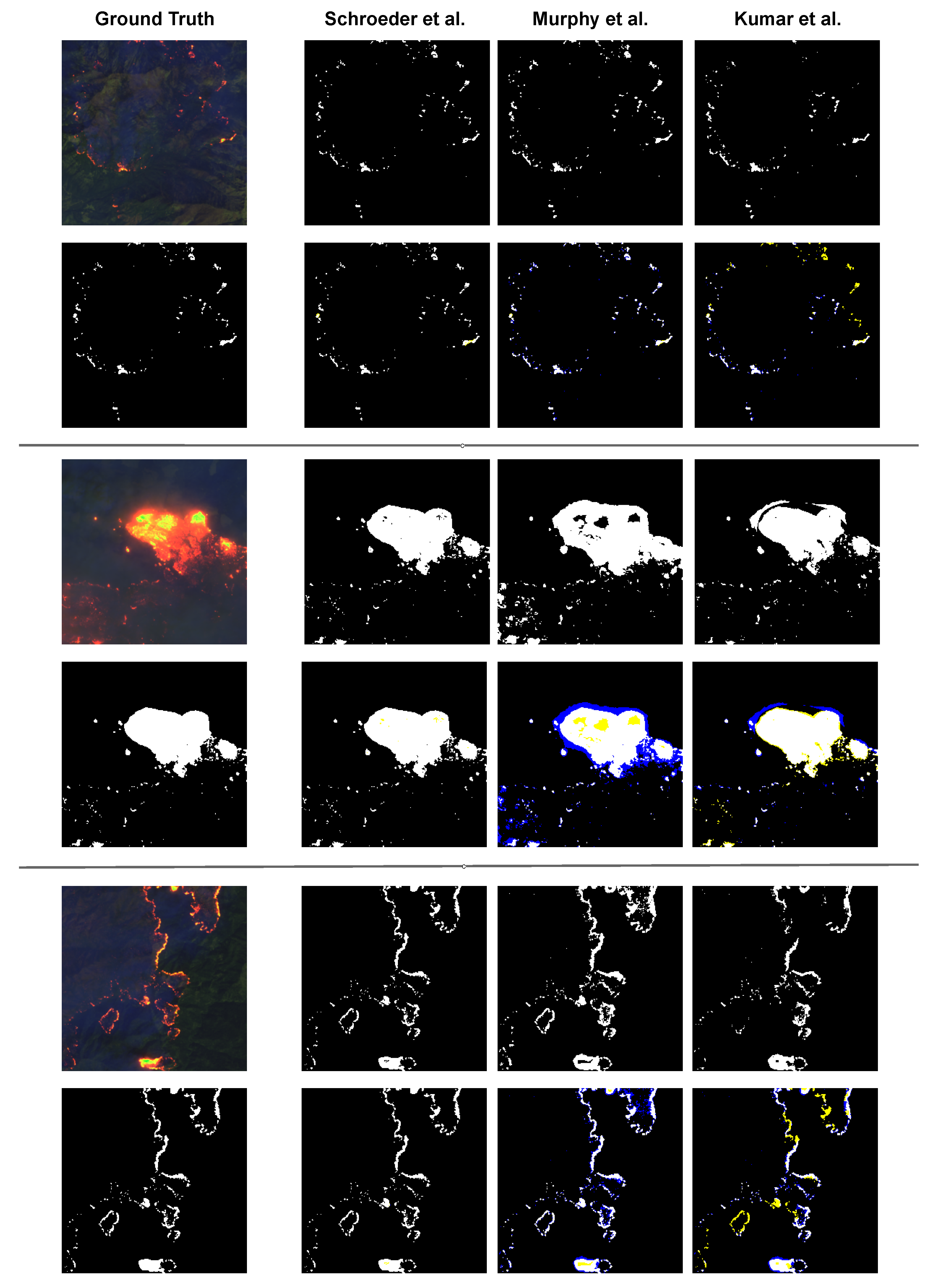
Figure 1. Visualization of wildfire detection using various existing thresholding methods on the Land8Fire dataset with three scenarios: scattered fires across the scene (top), a large, intense wildfire (middle), and a mid-stage fire beginning to spread (bottom). For each scenario: the 1st column displays the visible RGB image (1st row), followed by the ground truth (GT) mask (2nd row). The 2nd, 3rd, and 4th columns are the predicted mask (1st row), Schroeder et al. [22], Murphy et al. [12] and Kumar and Roy [13], respectively, followed by the highlighted misclassification including false negatives (shown in yellow) and false positives (shown in blue) (2nd row).
Remotesensing 17 02776 g001
Figure 2. Fire pixel distribution comparison across wildfire datasets. The top row illustrates the proportion of images containing at least one fire pixel, with Sen2Fire having only 14.18% fire-positive images, whereas all images in the ActiveFire and Land8Fire datasets contain fire. The bottom row highlights the differences in fire pixel distribution: Sen2Fire exhibits a highly skewed distribution, with most images containing either very few (<1) or a large number (>1000) of fire pixels, with no intermediate cases. ActiveFire retains a notable proportion of images with minimal fire pixels, while Land8Fire demonstrates a more balanced distribution across different fire pixel counts.
Remotesensing 17 02776 g002
Figure 3. Step 1: Manually annotate raw Landsat 8 images. Step 2: Identify fire clusters using OpenCV and create bounding boxes. Step 3: Expand bounding boxes if smaller than (256 + overlap) in either dimension, then crop them into 256 × 256 patches with a 220-pixel overlap.
Remotesensing 17 02776 g003
Figure 4. Quantitative metrics comparison: Visual illustration of differences between F1-score, precision, recall, mAccuracy, and IoU. The 1st row: Ground truth mask. The 2nd row: Predicted segmentation masks with various scenarios. The 3rd row: Visualization of True Positive, True Negative, False Positive and False Negative corresponding different predicted segmentation masks in the 2nd row. The 4th row: evaluation scores. In the first scenario, the predicted mask in the 1st column, it represents an overpredicted mask with expanded fire boundaries, resulting in high recall but lower precision due to excessive false positives. In the second scenario, the predicted mask in the 2nd column, it shows an underpredicted mask covering only part of the fire region, achieving perfect precision by avoiding false positives but suffering from low recall due to many missed fire pixels. In the third scenario, the predicted mask in the 3rd column, it demonstrates a model that fails to predict any fire pixels, resulting in deceptively high mAccuracy while all other scores remain at 0.0%. In the fourth scenario, the predicted mask in the 4th column, it shows a noisy prediction containing both false positives and false negatives.
Remotesensing 17 02776 g004
Figure 5. Visualization of segmentation results for different models on the Land8Fire dataset. The first row displays the visible image, followed by the ground truth (GT) mask in the second row. Subsequent rows correspond to predictions from various CNN- and transformer-based models as indicated on the left. The columns represent different fire scenarios: (1) small early-stage fires, (2) a small fire beginning to spread, (3) scattered fires distributed across the scene, and (4) a small but intense wildfire.
Remotesensing 17 02776 g005
Figure 6. Visualization of UNet outputs on the Land8Fire dataset using focal loss with varying gamma values. The first column shows the visible RGB image, followed by the ground truth (GT) mask. The remaining columns present predictions corresponding to different gamma values as labeled above. Each section illustrates a distinct wildfire scenario: (top) scattered fires across the scene, (middle) a small but intense wildfire, and (bottom) a large, intense wildfire cluster. In each section, the top row displays the predicted mask, while the bottom row highlights misclassified pixels—yellow indicates false negatives and blue indicates false positives.
Remotesensing 17 02776 g006
Figure 7. Visual representation on band comparison. (Left): (B2 (Blue) + B6 (SWIR1) + B7 (SWIR2)). (Right): (B4 (Red) + B3 (Green) + B2 (Blue)) (RGB).
Remotesensing 17 02776 g007
Table 1. Comparison between the existing datasets and our Land8Fire.
Aerial
Datasets
Dataset
Size
Fire Pixel
Distribution
Ground Truth
Annotation
Data Reliability
Sen2Fire2466High imbalanceSoftware (MOD14AI V6.1)Low, depend on the existing software
ActiveFire150,000+Imbalance (long tail)Automated (Algorithm-based)Low, depend on the existing algorithm
Land8Fire (ours)23,193Low imbalanceManual AnnotationHigh
Table 2. Full list of Land8Fire spectral bands.
Band NumberDescriptionWavelength (μm)Resolution
B1Coastal aerosol0.433–0.45330 m
B2Blue0.450–0.51530 m
B3Green0.525–0.60030 m
B4Red0.630–0.68030 m
B5Near Infrared (NIR)0.845–0.88530 m
B6Shortwave Infrared 1 (SWIR1)1.560–1.66030 m
B7Shortwave Infrared 2 (SWIR2)2.100–2.30030 m
B9Cirrus1.360–1.39030 m
B10Thermal Infrared 110.6–11.2100 m
B11Thermal Infrared 211.50–12.51100 m
Table 3. Performance of various methods on the Land8Fire dataset, including threshold-based (Schroeder, Kumar and Roy, and Murphy), CNN-based (FCN, UNet, PSPNet, UPerNet, and DeepLabV3+), and Transformer-based (Mask2Former and SegFormer) approaches. All deep learning models are trained with cross-entropy loss and evaluated using 5-fold cross-validation. The results for deep learning models are reported as (mean, standard deviation). As suggested in Pereira et al. [20], we only used the B7 (SWIR2), B6 (SWIR1), and B2 (Blue) bands.
MethodsBandsF1-ScoreRecallPrecisionmAccuracyIoU
Thresh
based
Schroeder{B1, B5, B6, B7}87.5882.9899.7691.4982.83
Kumar and Roy{B5, B6, B7}70.7591.9661.0895.8957.24
Murphy{B4, B5, B6, B7}74.2598.6262.4499.1161.45
Deep Learning
based
UNet{B2, B6, B7}94.49, 1.4293.28, 3.0195.79, 1.1196.62, 1.4989.58, 2.53
UPerNet{B2, B6, B7}80.76, 3.8074.42, 8.1183.83, 5.8987.17, 4.0565.35, 8.91
Mask2Former{B2, B6, B7}80.27, 5.2577.07, 6.0183.90, 5.8388.50, 3.0067.29, 7.16
SegFormer{B2, B6, B7}80.26, 6.1377.20, 7.9583.82, 5.4388.56, 3.9667.36, 8.31
DeepLabV3+{B2, B6, B7}78.96, 6.6975.76, 7.9982.54, 5.6887.84, 3.9865.62, 8.88
FCN{B2, B6, B7}64.99, 14.1255.77, 16.1379.54, 8.5677.85, 8.0649.38, 14.88
PSPNet{B2, B6, B7}64.77, 14.7755.34, 16.4980.38, 8.5077.64, 8.2449.15, 14.99
Table 4. Performance of UNet on a single fold of the Land8Fire dataset using B2 (Blue), B6 (SWIR1), and B7 (SWIR2) as input bands. Models were trained with cross-entropy and focal loss at varying gamma values. Due to training time constraints, results are reported on one fold only.
LossesGammaF1-ScoreRecallPrecisionmAccuracyIoU
Cross-Entropy95.6395.1397.7190.2386.17
Focal190.7785.497.5192.7083.38
292.6289.7395.8694.8586.28
489.9185.0995.5192.5381.72
Table 5. Performance of UNet on a single fold of the Land8Fire dataset using various spectral band combinations as input. All models were trained with cross-entropy loss. Due to training time constraints, results are reported on one fold only.
BandsF1-ScoreRecallPrecisionmAccuracyIoU
{B5, B6, B7}96.9997.2496.7398.6194.15
{B4, B5, B6, B7}96.3995.7197.3997.8593.31
{B1, B2, B4, B5, B6, B7}96.2094.4098.0897.1992.68
{B1, B2, …, B11}96.1798.8993.5999.4292.62
{B2, B6, B7}96.0096.5395.4898.2592.31
{B1, B5, B6, B7}95.1696.593.8698.2390.77
{B6, B7}94.9893.5296.4996.7590.44
{B2, B3, B4}32.7020.4781.3260.2219.55
Disclaimer/Publisher’s Note: The statements, opinions and data contained in all publications are solely those of the individual author(s) and contributor(s) and not of MDPI and/or the editor(s). MDPI and/or the editor(s) disclaim responsibility for any injury to people or property resulting from any ideas, methods, instructions or products referred to in the content.