Article

Towards Robust Hyperspectral Target Detection via Test-Time Spectrum Adaptation

Institute of Flight Systems, University of the Bundeswehr Munich, 85577 Neubiberg, Germany
*
Author to whom correspondence should be addressed.
Remote Sens. 2025, 17(16), 2756; https://doi.org/10.3390/rs17162756
Submission received: 16 May 2025 / Revised: 1 August 2025 / Accepted: 4 August 2025 / Published: 8 August 2025

Abstract

Target detection is a cornerstone task in hyperspectral image processing but faces significant challenges due to domain gaps. While statistical detectors like Constrained Energy Minimization (CEM) and Adaptive Cosine Estimator (ACE) are not prone to learned biases, in practice they still suffer from mismatches between the reference target spectrum and the spectral characteristics of the target in the test scene. We propose Test-time Adaptive Spectrum Refinement (TASR), a novel framework addressing this problem. TASR operates in an interpretable, lightweight, data-efficient manner, requiring only a single labeled source image of the target material. At test time, TASR dynamically refines the target spectrum to better align with the spectral properties of the test scene. This adaptive refinement enables detectors to effectively handle data with spectral variations, bridging the gap between the source and test spectra. To validate TASR, we conduct extensive experiments on established benchmarks and introduce a new dataset—ShadySunnyDiffuse (SSD)—which explicitly tests detector robustness to naturally occurring illumination changes. We further demonstrate the method’s versatility by applying it to camouflage detection and show compatibility with multiple statistical detectors. Our results establish TASR as a state-of-the-art approach in domain-adaptive hyperspectral target detection and target spectrum management.

1. Introduction

Effective hyperspectral target detection, whether using statistical or learned detectors, relies on the availability of a known target spectrum that accurately represents the material of interest. Traditionally, a straightforward approach is used: extracting the mean spectral vector from a labeled source image. However, hyperspectral target detection is inherently challenged by spectral variability [1,2,3], the phenomenon where a material’s spectral signature fluctuates due to external factors such as sensor noise, illumination, atmospheric conditions, occlusions, or even minor variations in the material’s surface properties [4]. Despite the well-documented significance of spectral variability [1,5,6,7], most research in this field operates under ideal conditions, where the target spectrum is extracted from the same image that is used for evaluating the detector [5,8,9,10,11,12].
This artificial setup is prevalent across widely used hyperspectral benchmarks such as HYDICE Urban [13], SanDiego [14], and Cuprite [15], which have been instrumental in the development of many state-of-the-art hyperspectral target-detection methods. Several influential papers in the field report AUC( P f , P d ) scores that consistently exceed 0.99 [8,9,10,12], suggesting near-perfect performance. However, these results may be misleading in real-world scenarios, where the source data from which a target spectrum is extracted is not identical to the test image. In practice, we must detect targets in new scenes and conditions [6], leading to spectral mismatches between the extracted reference spectrum and the target’s true spectral signature in the test image. This raises a crucial yet largely overlooked question: how robust are hyperspectral detectors when confronted with cross-scene scenarios?
In the field of visual-optical object detection, the challenge of detecting objects across different environments is extensively studied under the umbrella of domain adaptation. Researchers in this area focus on bridging the distribution gap between training and test datasets, ensuring models generalize to novel conditions. Several well-established benchmarks assess cross-domain generalization, including Cityscapes [16] to Foggy Cityscapes [17] for evaluating robustness to adverse weather conditions, Sim10k [18] to Cityscapes for measuring the ability to transition from synthetic to real-world data, and visual-optical to infrared benchmarks [19,20] for cross-spectrum adaptation. However, no comparable benchmarks exist for hyperspectral target detection, primarily due to the unique challenges of working with hyperspectral data cubes, which are difficult to collect and store at scale. In fact, widely used hyperspectral datasets often consist of a single data cube, which fundamentally prevents any systematic study of cross-scene adaptation. This scarcity implies that addressing domain adaptation in hyperspectral target detection requires not only the development of robust detectors but also frugal algorithms that can adapt to new environments without access to extensive datasets. Inspiration can be drawn from works in one-shot, unsupervised domain adaptation for object detection, which demonstrate that even a single unlabeled test-domain image can significantly boost model performance [21,22,23,24]. While primarily explored in the visual-optical context, the premise of one-shot, unsupervised domain adaptation holds strong potential for hyperspectral target detection, where data scarcity is a key challenge.
While domain gaps in visual-optical object detection are often categorized into different levels, such as image-level, object-level, or pixel-level, we argue that in hyperspectral target detection, the primary cause of failure is the mismatch between the extracted target spectrum and the spectral characteristics of the test scene. This issue is particularly evident in statistical detectors like Constrained Energy Minimization (CEM), which directly processes the test image and relies solely on the extracted spectral vector as prior information [12]. Unlike deep methods, which may fail due to learned biases [25,26], statistical detectors break down primarily because their target spectrum no longer aligns with the spectral distribution of the test environment. Rather than adapting entire models or images, we propose an alternative approach: adapting the target spectrum itself. Instead of relying on the extracted source spectrum, TASR finds a reference spectrum directly within the test image, bridging spectral shifts and improving detection without altering the underlying detector.
Our contributions can be summarized as follows. (1) We introduce the problem of cross-scene target detection in hyperspectral imagery, emphasizing its importance and highlighting the shortcomings of current evaluation practices. (2) We propose new cross-scene domain adaptation benchmarks for hyperspectral target detection, enabling more realistic assessments of detector performance under spectral variability. (3) We introduce the novel research area of target spectrum adaptation, shifting the focus to directly adapting target vectors at test time. (4) We present TASR, the first framework for test-time target spectrum adaptation, designed to mitigate spectral mismatches and improve hyperspectral target detection across diverse real-world environments in an interpretable and data efficient manner.
By shifting the research focus towards target spectrum adaptation and realistic evaluation methodologies, we aim to bridge the gap between lab conditions and practical deployment scenarios—such as airborne target monitoring via UAVs in unfamiliar environments—ultimately advancing the field of hyperspectral target detection towards more robust and generalizable solutions.

2. Materials and Methods

2.1. Test-Time Adaptive Spectrum Refinement

The Test-time Adaptive Spectrum Refinement (TASR) framework addresses hyperspectral target detection under domain shift, where spectral signatures of the same material may vary significantly across scenes due to changes in lighting, atmospheric conditions, or background composition. TASR assumes access to a labeled source image containing known instances of a target material and an unlabeled test image where the goal is to detect occurrences of the same material. Rather than relying on the target spectrum from the source image—which may be unreliable in the new scene due to spectral variability—TASR adaptively estimates a target spectrum directly from the test image by selecting a set of pixels whose average spectrum is likely to correspond to the material of interest.
To identify such a pixel set, TASR uses a discrete genetic algorithm [27] (GA)—a population-based search heuristic inspired by biological evolution. Genetic algorithms are particularly well-suited for discrete optimization problems where the search space is combinatorial, as in the selection of subsets of pixels from a high-dimensional hyperspectral image. In TASR, each candidate solution (or genome) is a set of 10 pixel indices from the test image, with replacement (i.e., duplicates allowed). The core hypothesis is that if the average spectrum of these selected pixels enables strong target detection in the source image—when used as input to a fixed detector such as Constrained Energy Minimization (CEM) [28]—then those pixels are likely to be true instances of the target in the test image.
The optimization begins with a randomly initialized population of 30 candidate solutions. Over 50 generations, this population is iteratively refined through selection, crossover, mutation, and fitness evaluation. Selection is performed using tournament selection [29] with a tournament size of 5: five candidates are randomly sampled from the current population, and the one with the highest fitness is selected. This process is repeated until 15 parents—half the population—are chosen. This number ensures a balance between selection pressure and genetic diversity, preventing premature convergence while enabling steady progress [30]. To preserve high-quality solutions, the best individual from the previous generation is copied unchanged to the next (elitism) [31]. The remaining 29 offspring are generated via uniform crossover, where each gene (i.e., pixel index) in a child has a 50% chance of being inherited from either parent. Since the number of required offspring exceeds the number of parent pairs, some parents contribute multiple times and some pairs are reused.
To promote exploration and prevent stagnation, mutation is applied to all offspring. With a mutation rate of 0.25, 25% of the genes in each individual are replaced with new, randomly selected pixel indices from the test image. This mutation rate was selected to maintain sufficient diversity while preserving promising solutions. After crossover and mutation, all individuals in the new generation—including the elite—are evaluated using a fitness function that combines detection accuracy and spectral distinctiveness. The population size remains fixed at 30 throughout, and this evolutionary loop continues for 50 generations.
Fitness evaluation is central to TASR. For each candidate, the average spectrum of the selected pixels is computed and used as a pseudo-target for CEM detection on the labeled source image. The performance of this detection is quantified using the area under the curve (AUC) of the ROC curve, denoted F AUC . The AUC is calculated using the trapezoidal rule [32] from the detection ( P d ) and false alarm ( P f ) probabilities across thresholds:
F AUC = i = 1 n 1 ( P f i + 1 P f i ) · ( P d i + P d i + 1 ) 2 .
This term encourages the selection of pixel sets whose spectra produce high detection accuracy when used in a cross-scene manner. However, relying solely on this term can lead the optimizer to exploit artifacts: for example, it may select background pixels whose linear combination coincidentally resembles the source target spectrum, yielding high performance in the source image without truly representing the target in the test image.
To address this limitation, TASR introduces an auxiliary term to promote spectral separability from the test image background. Specifically, it computes the spectral angle mapper (SAM) between the candidate target spectrum t and the average background spectrum b , defined as:
F sep = arccos t b t b ,
where · denotes the Euclidean norm. This angle lies in [ 0 , π ] , with larger values indicating greater angular separation and, hence, better discriminability. By including this term in the fitness function, TASR discourages degenerate solutions that match the source image but lack distinctiveness from the test background.
The final fitness function combines the detection and separability terms as:
F total = F AUC + w 1 · F sep ,
where w 1 is a hyperparameter controlling the trade-off between the two objectives. Unless otherwise specified, we use w 1 = 0.1 , which was found to yield stable performance across datasets.
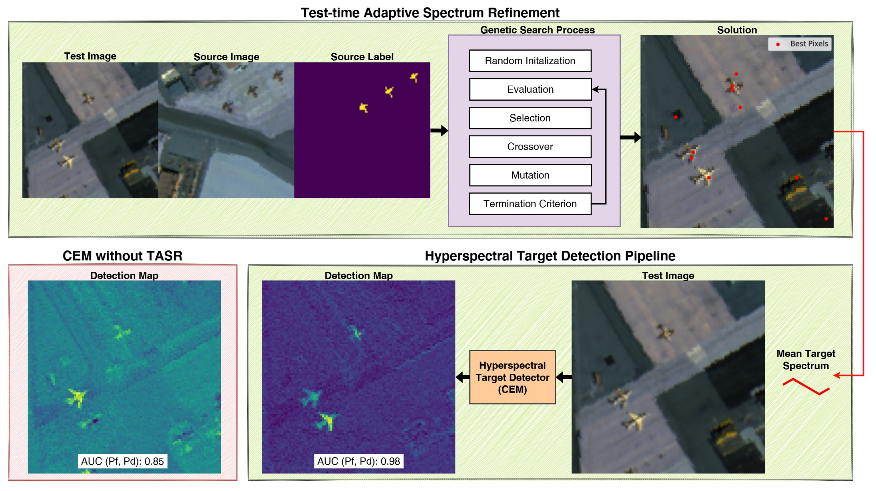
Upon completion of the 50-generation optimization, the candidate with the highest fitness is selected. The average spectrum of its selected pixels serves as the refined, scene-adapted target spectrum. This spectrum is then used to perform detection in the test image using CEM. An example of the evolutionary process is visible in Figure 1. By adapting the target representation to the spectral characteristics of the test image, TASR improves robustness to spectral variability and effectively bridges the domain gap without requiring any test labels.
To ensure consistent search behavior across datasets of varying resolutions, all test images are resized to a fixed resolution of 100 × 100 pixels prior to optimization. This step also improves computational efficiency and avoids the need for dataset-specific hyperparameter tuning. The full, high-level pipeline is visualized in Figure 2.

2.2. Datasets

Hyperspectral target detection has relied heavily on well-established benchmark datasets such as San Diego [14] and Urban [13]. However, these datasets are often limited in size, typically consisting of only one or a few images. When datasets contain multiple images, they are often treated as separate test cases, such as San Diego 1 and San Diego 2, rather than being evaluated in a more integrated manner. This practice typically involves training and/or tuning detectors on the same image used for the final test, which leads to overly optimistic results. To address these limitations, we construct cross-scene domain adaptation benchmarks. This setup, inspired by benchmarks in visual-optical object detection such as Synscapes → Cityscapes and Cityscapes → Foggy Cityscapes, enables the evaluation of detector robustness across varying contexts. In hyperspectral detection, this involves extracting target spectra from one image (source) and performing cross-scene evaluations on another (test), thereby reflecting real-world challenges. Below, we further detail the datasets used to implement this approach.

2.2.1. SanDiego1↔SanDiego2

The SanDiego1 and SanDiego2 datasets are derived from images of the publicly available hyperspectral imaging (HSI) dataset collected by the Airborne Visible/Infrared Imaging Spectrometer (AVIRIS) over San Diego Airport, CA, USA, on 9 November 2011 [14]. Both datasets have a ground sampling distance of 3.5 m and include 189 spectral bands after removing low-quality bands affected by water vapor absorption and low signal-to-noise ratios (SNR). Each data cube consists of 100 × 100 pixels, with three airplanes as the targets of interest. SanDiego1 contains 64 target pixels (0.58% of the image), while SanDiego2 includes 134 target pixels (1.34% of the image). For the benchmark, each dataset alternates as the source for extracting hyperspectral target spectra and the test dataset to ensure comprehensive evaluation.

2.2.2. Camo1↔Camo2

The Camo1 and Camo2 datasets consist of hyperspectral images collected using the AFX17 sensor (Specim, Spectral Imaging Ltd., Oulu, Finland), covering a spectral range of 900–1700 nm with an 8 nm spectral resolution, resulting in 224 spectral bands [33]. Both datasets have a spatial resolution of 550 × 550 pixels and contain a single forest camouflage net as the target of interest. The net was designed to provide concealment in both the visual-optical and far infrared. Dataset collection was performed in a grassland/forest area near a road on the University of the Bundeswehr Munich campus at an altidude of 60 m, while the Camo2 dataset was recorded in a similar grassland/forest environment at a testing site near Storkow at an altidude of 50 m. Camo1 contains 429 target pixels (0.14% of the image), and Camo2 contains 627 target pixels (0.21% of the image). As with the SanDiego benchmark, evaluations are performed in both directions.

2.2.3. ShadySunnyDiffuse

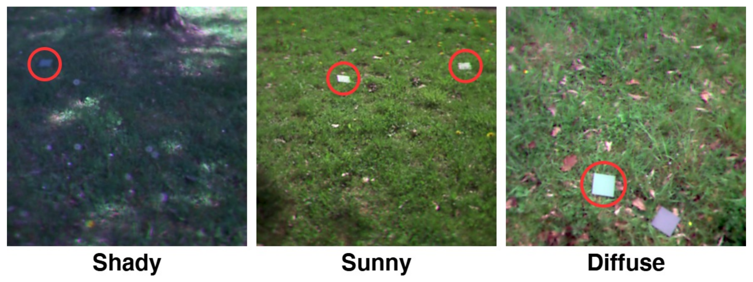
The ShadySunnyDiffuse (SSD) dataset comprises three hyperspectral images captured using a Ultis X20 Plus camera (Cubert GmbH, Ulm, Germany). Each image has a spatial resolution of 410 × 410 pixels and contains 164 spectral bands covering the VNIR range from 350 to 1000 nm. The dataset was specifically designed to evaluate the robustness of hyperspectral target-detection methods under naturally varying lighting conditions.To construct this dataset, identical 3D-printed green plastic targets of size 10 × 10 pixels were placed into three distinct scenes. The first image, referred to as the “shady” condition, includes a single target placed beneath a tree on a bright sunny day, resulting in under-illumination due to shadow cover. The second image, termed the “sunny” condition, features two green targets placed in a sunlit grassy field. This configuration was chosen to introduce over-illumination and to test the detector’s ability to identify multiple instances of the target. The third image, referred to as the “diffuse” condition, was acquired on a cloudy day, resulting in soft, uniform lighting. In this scene, a grey plastic decoy target of identical size was placed alongside the green target to evaluate the detector’s discriminative capacity in the presence of visually similar but spectrally distinct distractors. The shady image contains 261 target pixels (0.1553% of the image), the sunny image contains 509 target pixels (0.3028%), and the diffuse image contains 1372 target pixels (0.8162%). As with the SanDiego and Camo benchmarks, we perform evaluations in all possible source-target directions, resulting in six distinct testing conditions. This setup supports comprehensive cross-scene assessment under diverse illumination and contextual variability. The images in the SSD dataset are presented in Figure 3.

2.3. Quality Metrics

In hyperspectral target detection, the evaluation of detection performance relies on several key metrics derived from the receiver operating characteristic (ROC) curves. These metrics assess different aspects of a detector’s effectiveness, detectability, and robustness.
Three fundamental AUC metrics are considered. First, AUC ( P f , P d ) measures effectiveness, a direct measure of practical utility. It evaluates how well the detector balances the probability of false alarms ( P f ) and the probability of detection ( P d ). A higher value (closer to 1) indicates a better trade-off, meaning the detector can achieve high detection rates while keeping false alarms low. Second, AUC ( τ , P d ) assesses detectability, focusing on how well the detection threshold ( τ ) separates targets from the background. A higher value (closer to 1) means that as the threshold varies, the detector consistently identifies targets while ignoring non-targets. This metric reflects how reliably the system distinguishes true targets from their surroundings. Third, AUC ( τ , P f ) captures false alarm sensitivity, measuring how the false alarm rate changes as the threshold ( τ ) varies. A lower value (closer to 0) is desirable, as it indicates that increasing the threshold effectively reduces false alarms.
In addition to these individual metrics, two composite metrics provide a more comprehensive assessment. The overall quality metric, AUC O A , is defined as:
AUC O A = AUC ( P f , P d ) + AUC ( τ , P d ) AUC ( τ , P f ) .
This metric combines effectiveness, detectability, and false alarm rate into a single value, with a higher score (ideal = 2) indicating strong performance across all aspects. Meanwhile, the signal-to-noise power ratio metric, AUC S N P R , is given by:
AUC S N P R = AUC ( τ , P d ) AUC ( τ , P f ) .
This ratio evaluates the robustness of the detection process by comparing detectability to false alarms, where a higher value (ideal = + ) indicates a strong ability to suppress false alarms while maintaining high detectability.
Beyond detection performance, computational efficiency is a critical consideration in hyperspectral target detection, as many algorithms are prohibitively expensive for real-time or large-scale applications [34]. Therefore, we also include inference time (measured in seconds) as an additional metric to assess the feasibility of methods in practical scenarios.

2.4. Experimental Details

The TASR framework is implemented in Python using the PyGAD library. All images are normalized. Key hyperparameters—including population size, number of generations, crossover rate, and mutation rate—were carefully selected to balance computational efficiency and performance, and are commonly used in discrete genetic algorithm literature. A comprehensive list of hyperparameters is provided in Appendix A. All benchmarks were conducted on an RTX 4090 GPU and an Intel i9-14900KF processor. To ensure fair and consistent comparisons, we reproduced all benchmarked methods within our framework, carefully verifying that our implementations matched the original authors’ reported results. Methods that do not use TASR use a hyperspectral target spectrum that is extracted as the mean spectrum from the source label map. Standard deviations are reported based on 25 independent runs. The complete code and datasets are available at https://github.com/RobinGerster7/TASR (accessed on 3 August 2025). The experiments were conducted using commit cd3c2c7 of the repository.

3. Results

In this section, we evaluate our proposed TASR method alongside several statistical hyperspectral target detectors on two newly introduced cross-domain benchmarks: SanDiego and Camo. We report detection performance using the metrics in Table 1, and include Oracle variants that use the true target spectrum from the test scene to establish an upper-bound for each method. For completeness, we also provide additional tables in Appendix B where the AUC metrics are computed over a low false positive rate (FPR) range of 10 4 to 10 2 , which is sometimes desirable in scenarios where false positives are particularly undesirable. Quantitative comparisons are complemented by visual detection maps to qualitatively assess detector performance. We organize our analysis into several experiments. First, we benchmark TASR against existing detectors on each dataset to demonstrate its cross-domain robustness. Next, we show that TASR can be used as a plug-and-play refinement module that enhances a wide range of detectors by adapting their target spectrum at test time. We then study TASR’s convergence behavior, demonstrating that its fitness function is a reliable proxy for downstream detection quality. This is followed by a sensitivity analysis on genome length to assess the trade-offs between expressive power and optimization complexity. Finally, we conduct an ablation study to evaluate the impact of the separability term in the fitness function, which promotes the selection of discriminative target pixels.

3.1. SanDiego1↔SanDiego2

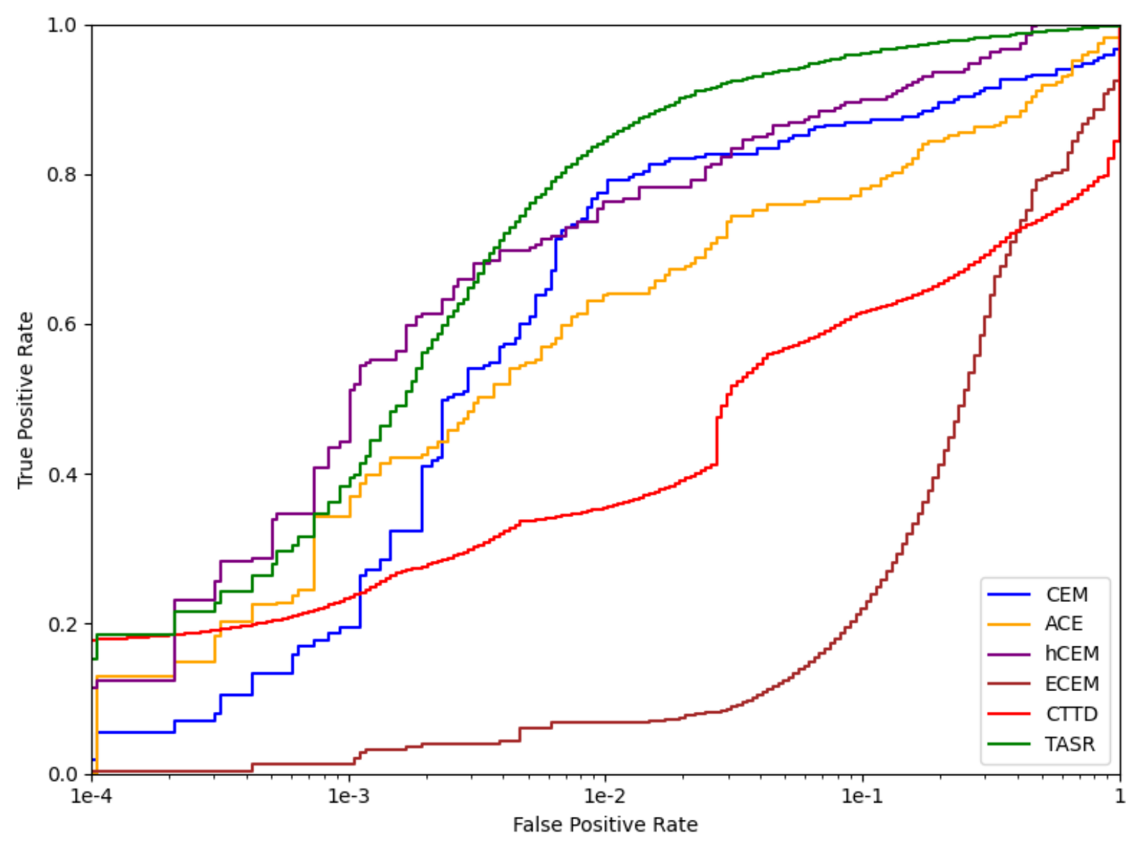
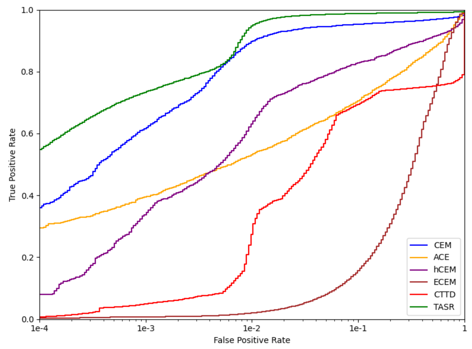
Table 2 presents the performance of various hyperspectral target detectors on the SanDiego benchmark, highlighting the substantial performance drop when transitioning from an same-scene to a cross-domain evaluation. ECEM and CTTD, which achieve AUC( P f , P d ) scores above 0.99 in same-scene evaluations, drop sharply to 0.670 and 0.722, respectively, in cross-domain settings. This reduction indicates that despite their strong same-scene performance, these detectors struggle with domain shifts induced by target spectrum variability. Although all methods degrade in cross-domain settings, hCEM remains relatively robust with an AUC( P f , P d ) of 0.965. In contrast, TASR significantly improves CEM’s cross-domain performance, increasing its AUC( P f , P d ) from 0.92 to 0.978—the highest among all tested methods. This is further supported by Figure 4, where TASR maintains a consistently high true positive rate across the range of false positive rates, unlike methods such as CEM and ECEM that exhibit early drop-offs. We emphasize AUC( P f , P d ) as the practical and interpretable performance measure, as other metrics, such as AUC( τ , P f ), can be misleading in assessing detection capability. For instance, ACE achieves the lowest AUC( τ , P f ), suggesting a low false positive rate, but this is due to its failure to detect targets rather than superior selectivity. A similar argument holds for AUCSNPR. Such cases highlight the need for a holistic evaluation and qualitative results. Inference time varies significantly across methods. CEM is the most efficient detector, requiring just 0.010 s per inference, making it ideal for real-time applications. In contrast, TASR achieves the best cross-domain performance but requires 4.225 s per inference, making it one of the slowest among the benchmarked detectors—surpassed only by ECEM, which takes 4.755 s. Despite TASR’s higher inference time, all detectors evaluated in this study are relatively fast compared to many well-known hyperspectral methods. For instance, CSCR [35], which utilizes sparse representations, MLSN [36], a meta-learning-based Siamese network, and the autoencoder ULMMDL [37] are known to be significantly slower.
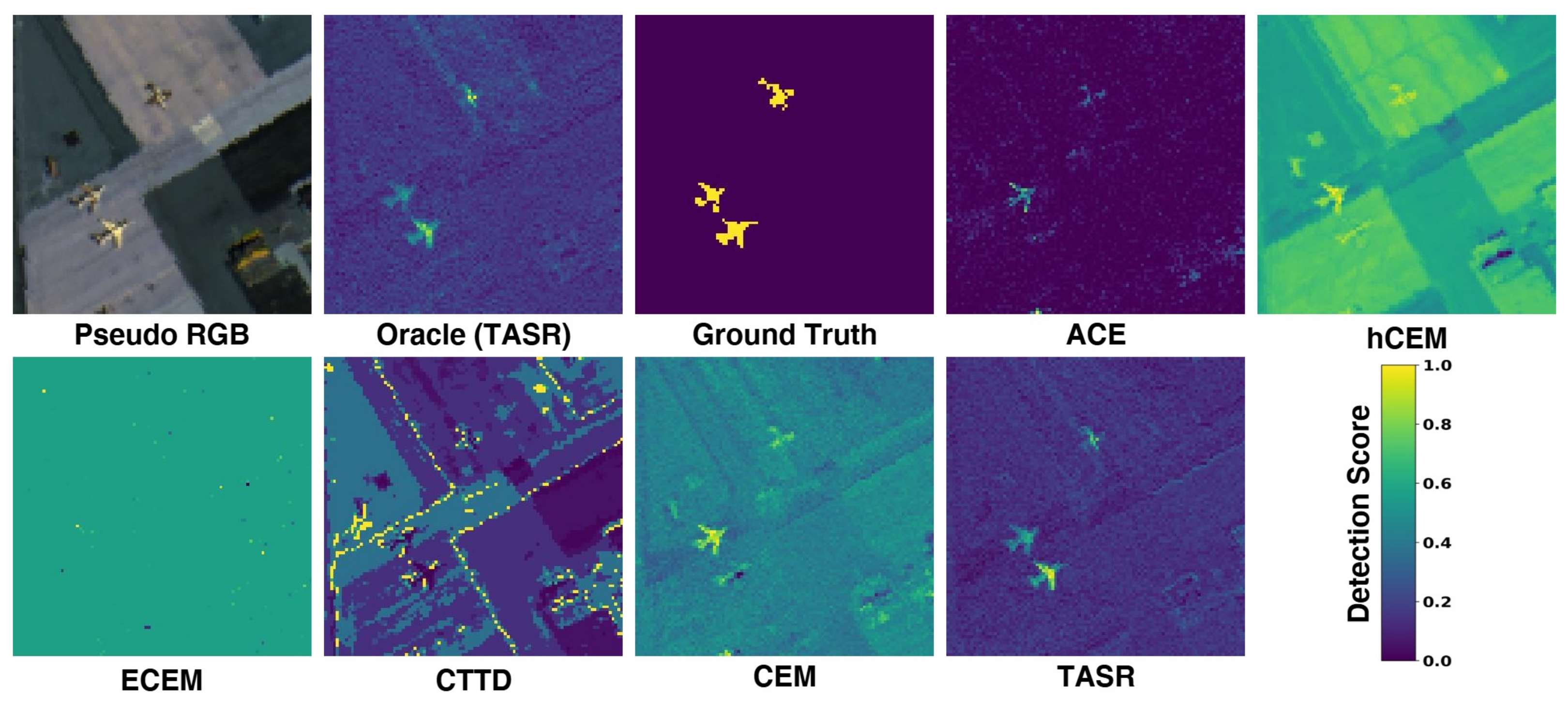
To complement the numerical analysis, we present detection maps in Figure 5, offering a side-by-side visual comparison of all evaluated methods. TASR stands out by producing the most accurate detection map, effectively delineating targets with minimal false positives. Although hCEM achieves a marginally higher AUCOA and a comparable but slightly lower AUC( P f , P d ), its detection maps exhibit a high false positive rate, resulting in cluttered outputs where not all airplanes are distinctly visible. In contrast, ACE, despite minimizing false positives, fails to generate a meaningful detection map, as its excessive selectivity prevents effective target localization. The failure of ECEM and CTTD to generalize across scenes is evident in their detection maps, where no discernible airplanes appear. Compared to the baseline CEM, TASR not only improves target delineation but also yields the cleanest detection map, with a darker, more uniform background that minimizes noise. These qualitative findings reinforce TASR’s superiority and highlight the importance of carefully managing target spectra in cross-domain target detection.

3.2. Camo1↔Camo2

The Camo benchmark poses a particular challenge due to the presence of camouflaged targets, which make it difficult to distinguish them from the background. As shown in Table 3, ECEM and CTTD achieve the lowest AUC( P f , P d ) values at 0.534 and 0.542, respectively, indicating their vulnerability to domain shifts. Unlike in the SanDiego experiment, hCEM also exhibits a substantial decline in effectiveness falling to 0.765, suggesting that its robustness is not consistent across different detection tasks. Standard CEM, however, remains relatively stable at 0.954, making it the most robust among the tested baselines. Notably, TASR outperforms all methods, achieving 0.997 AUC( P f , P d ) while also exhibiting a low false positive rate and high detectability. This is visually evident in Figure 6, where TASR consistently dominates the ROC curve across all false positive rates. Consequently, TASR achieves the highest AUCOA by a wide margin. While the SanDiego dataset consists of 100 × 100 images with 189 spectral bands, the Camo dataset features 550 × 550 images with 224 spectral bands, significantly increasing computational demands. Despite this, CEM remains the fastest method, requiring only 0.085 s to process the larger data cubes, while ECEM is the slowest at 33.875 s. TASR benefits from an efficient design: during the genetic optimization process, image resolution is reduced to 100 × 100, ensuring that the search process scales linearly with the number of spectral bands rather than cubically with spatial and spectral resolution. However, the increased spectral dimensionality (224 bands compared to 189 in SanDiego) during optimization, along with the final hyperspectral target detection step—which operates on the full 550 × 550 × 224 data cube after spectrum refinement—introduces additional computational overhead, increasing inference time from 4.225 s in the SanDiego benchmark to 7.124 s.
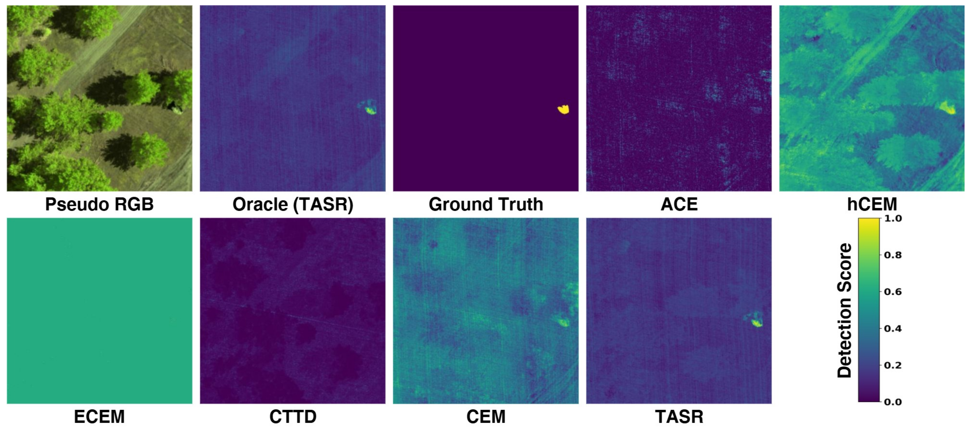
The detection maps in Figure 7 provide further insights into these trends. ACE, ECEM, and CTTD fail to detect the target entirely, confirming their poor robustness in cross-domain camouflage detection. CEM and hCEM show partial detection capability, but their outputs contain high false positive rates, making them less reliable and targets hard to locate. TASR produces a detection map closely resembling the Oracle (CEM), successfully delineating the camouflage net while minimizing background noise. These findings highlight TASR’s effectiveness in bridging spectral domain shifts, positioning it as the most suitable detector for cross-scene camouflage detection.

3.3. ShadySunnyDiffuse

The ShadySunnyDiffuse (SSD) dataset introduces domain shifts commonly observed in outdoor remote sensing, particularly those caused by variations in illumination conditions such as shading, direct sunlight, and diffuse lighting. These changes significantly alter the spectral appearance of materials, complicating target detection. As shown in Table 4, this illumination-induced spectral variability leads to a marked drop in detection performance for most statistical detectors. ECEM and CTTD are especially sensitive, with AUC( P f , P d ) scores falling to 0.641 and 0.734, respectively, confirming their limited capacity to generalize across different lighting conditions. While CEM demonstrates greater robustness—maintaining AUC( P f , P d ) values above 0.96—their performance still suffers due to elevated false positive rates. Once again, it can be observed in Figure 8 that TASR clearly dominates across various thresholds for false positive rates. Notably, hCEM achieves the highest AUC( τ , P d ) at 0.764, suggesting high detectability, but this comes at the cost of significant background activation, as evidenced by its high AUC( τ , P f ) of 0.606. In contrast, TASR achieves the highest AUC( P f , P d ) of 0.987, nearly matching Oracle performance, which indicates that it effectively compensates for spectral distortions introduced by lighting shifts. Furthermore, TASR maintains a low AUC( τ , P f ), demonstrating effective suppression of false positives. The method’s strong performance across all evaluated metrics, combined with its relatively low variance, further underscores its suitability for real-world deployment in dynamic, uncontrolled environments.
The detection maps in Figure 9 further validate the effectiveness of TASR under challenging lighting conditions. While the target spectrum is derived from the diffuse scene—where spectral signatures are clean and uncorrupted—the test image originates from the sunny condition, where targets are spectrally distorted due to over-illumination. This type of corruption is prevalent in aerial hyperspectral sensing applications and often leads to severe detection degradation. As observed, traditional detectors like ACE, ECEM, and CTTD fail to localize targets accurately, either missing them entirely or producing overly sparse maps. CEM and hCEM produce moderate results, but their detection maps remain noisy, with considerable background activation. In contrast, TASR generates a highly focused detection map that closely resembles the Oracle output, successfully suppressing background noise while clearly delineating the target. These results illustrate TASR’s capacity to adapt to real-world spectral distortions introduced by illumination which is of practical value in field-deployable systems.

3.4. Spectra Analysis

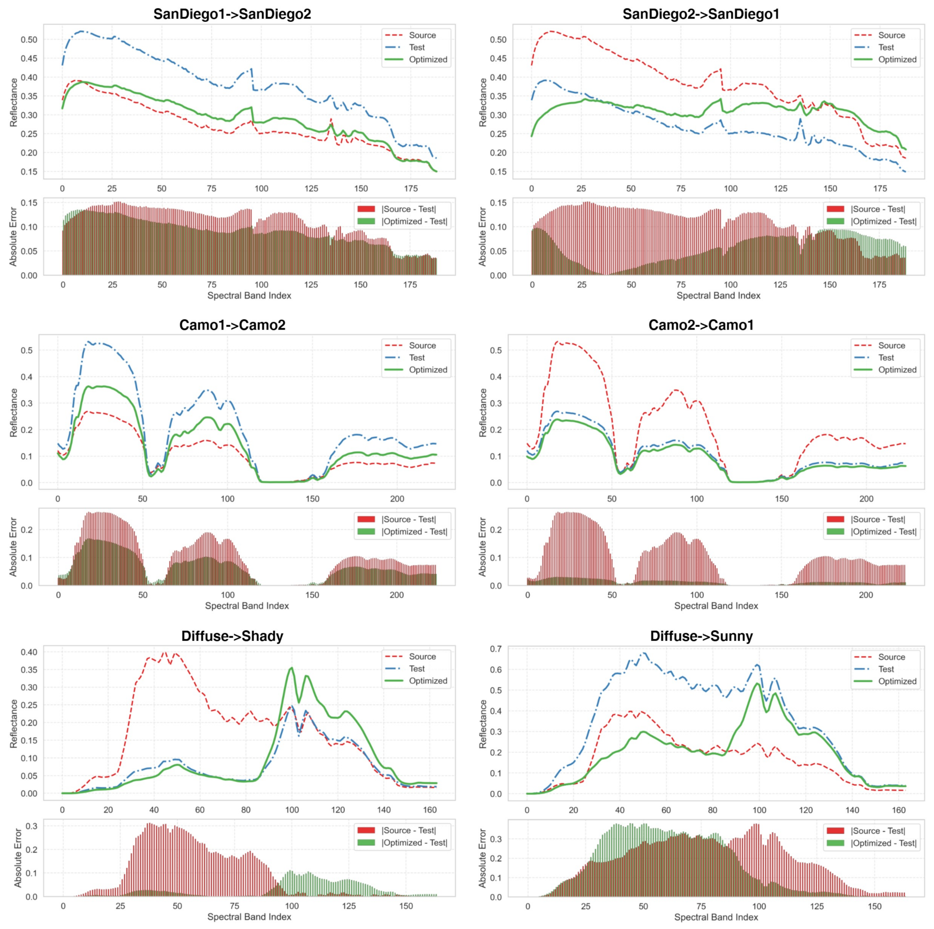
TASR is designed as a method to optimize target spectra. As demonstrated in previous sections, the optimization process consistently yields favorable downstream performance gains—quantitatively measured through metrics such as AUC( P f , P d ) and visualized via ROC curves. Similarly, qualitative improvements can be observed through inspection of the resulting detection maps. While these results suggest that the spectrum refinement process is effective, it is also important to examine how the optimized spectra compare to both the original source spectra and the spectra extracted from the test domain.
In Figure 10, we conduct this analysis by comparing spectral curves from the SanDiego and Camo datasets in both source-to-test directions, as well as from the ShadySunnyDiffuse (SSD) dataset in the diffuse-to-sunny and shady subsets. The latter condition reflects a practical use case: a high-quality reference spectrum is collected under diffuse lighting, but the target appears under drastically different illumination, introducing significant spectral variability. Beyond side-by-side visualizations of the spectra, we also plot the absolute error per channel to better highlight spectral differences. Across all cases, a consistent trend is observed: the TASR-optimized spectra tend to more closely resemble the test spectra than the original source spectra do. This is particularly evident in the reduced channel-wise error in the optimized–test comparisons relative to source–test. To quantify this observation, we compute the mean absolute error (MAE), mean squared error (MSE), and cosine similarity (Cos) between each pair of spectra across the entire dataset. The results, summarized in Table 5, indicate substantial improvements in MAE and MSE, with reductions ranging from 33.4% to 80.3%. Improvements in cosine similarity, which captures spectral shape rather than magnitude, are more nuanced: a 13.9% improvement is observed for the SSD dataset, whereas gains in Camo are modest (0.6%), and a slight reduction (−0.7%) is seen in SanDiego, which may be considered negligible in practice. We note, however, that the notion of what constitutes a “refined” spectrum remains underexplored in the literature. Further research is warranted to establish robust criteria for spectrum refinement and to better understand which spectral characteristics most influence detection performance.

3.5. Improving Detection Across Methods

TASR introduces the concept of target spectrum adaptation, a broader research direction that extends beyond individual detectors. In theory, a perfect target spectrum adaptation algorithm could enable statistical hyperspectral detectors to achieve Oracle performance. Consequently, TASR is expected to enhance various detectors beyond CEM by offering a more precise approximation of the target spectrum in novel scenes.
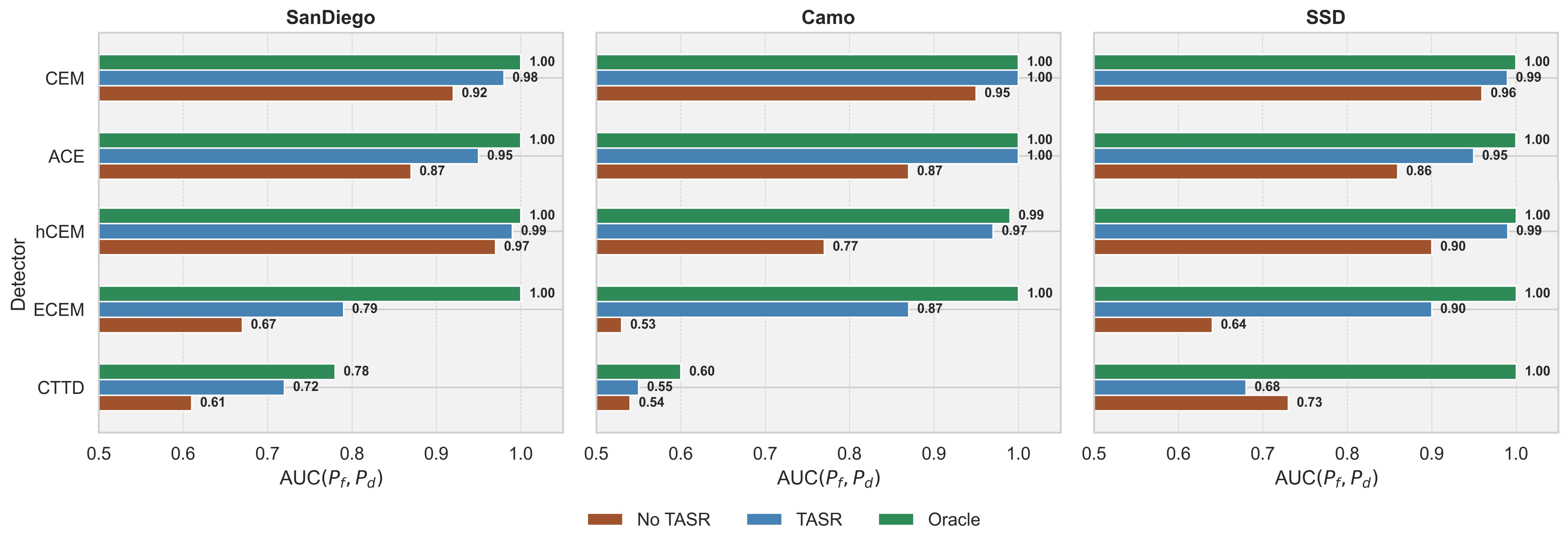
To validate this hypothesis, a systematic experiment is conducted where the default hyperspectral target detector (CEM) is sequentially replaced with each of the benchmarked methods. Performance is evaluated across all datasets. The results in Figure 11 confirm that using TASR leads to a notable and consistent improvement in detection effectiveness. Even in the SanDiego dataset, where some detectors already perform well without additional test-time spectrum adaptation, TASR provides meaningful gains. The most substantial improvements occur in methods with limited generalization capabilities. For example, ECEM in the Camo dataset improves dramatically, with AUC( P f , P d ) increasing from 0.53 (a completely monotone detection map) to 0.87. Similarly, hCEM in the Camo dataset rises from 0.77 to 0.97, and ECEM in the SanDiego dataset increases from 0.67 to 0.79.
Interestingly, for detectors that are already relatively robust in the Camo dataset, such as CEM and ACE, TASR enables AUC( P f , P d ) values to reach or exceed 0.995, further underscoring its ability to refine and enhance detection performance. However, an exception is observed with the CTTD, where TASR fails to yield the expected improvement. This discrepancy may arise from CTTD’s strong dependence on hyperparameters, limiting its ability to generalize effectively. Moreover, even the Oracle for CTTD yields suboptimal results, suggesting that the issue may lie with the detector itself rather than TASR. This introduces an important consideration: TASR functions as a framework that adapts the target spectrum, but its effectiveness also depends on the characteristics of the detector it is applied to. While TASR consistently enhances performance across most tested cases, its effectiveness is influenced by the detector’s ability to leverage the refined target spectrum. Therefore, applying TASR requires careful consideration, especially for methods with rigid model assumptions or substantial hyperparameter sensitivities such as CTTD.
While CEM serves as the default detector within TASR, it is not the top-performing method on the SanDiego dataset, where it is slightly outperformed by hCEM. Nonetheless, CEM exhibits the most stable performance across varying conditions and offers computational efficiency and simplicity, making it a suitable general-purpose choice. Overall, our findings demonstrate that TASR provides significant performance improvements across diverse detectors and datasets, reinforcing the potential of target spectrum adaptation as a promising direction for advancing cross-domain hyperspectral target detection.

3.6. Convergence Study

We perform a convergence analysis to evaluate the suitability of our fitness function as a proxy for final detection performance. Figure 12 shows the evolution of fitness (left) and AUC( P f , P d ) (right) across generations for three benchmark datasets. The strong correlation between the two curves confirms that the fitness function reliably predicts downstream detection quality. Across all datasets, TASR rapidly approaches or surpasses the baseline CEM performance within the first 10 generations and stabilizes by around 25 generations. This suggests that the number of generations can be reduced without significantly compromising performance—an important consideration for time-sensitive applications. These results demonstrate that TASR not only converges efficiently but also leverages a well-aligned objective function.

3.7. Genome Length Sensitivity

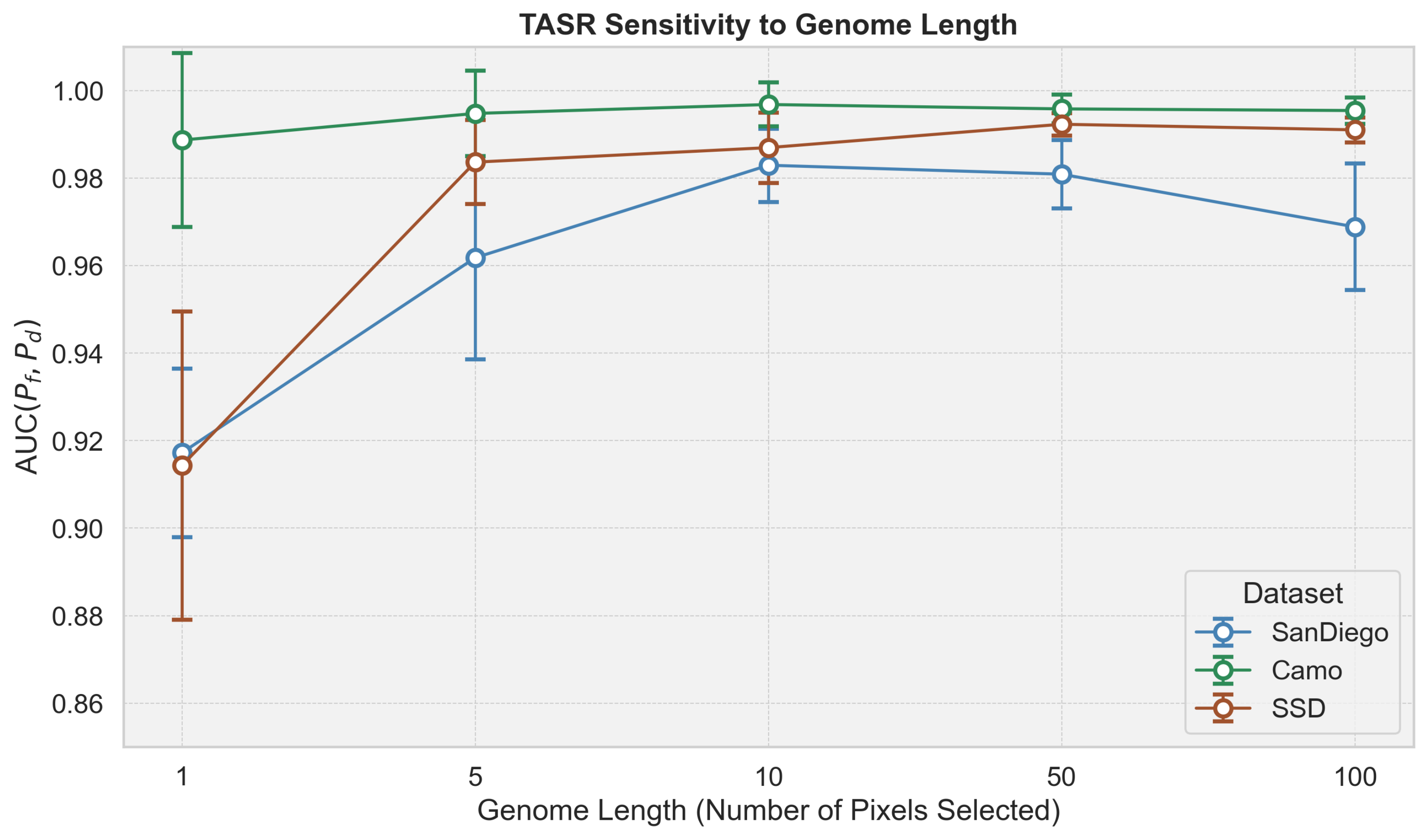
We conduct a sensitivity analysis to evaluate the effect of genome length—i.e., the number of pixels selected for spectrum refinement—on TASR’s detection performance. By default, we set the genome length to 10, but it is important to understand the implications of this design choice. As shown in Figure 13, very small genome lengths lack sufficient expressive power to construct effective linear combinations. In particular, a genome length of 1 consistently yields the lowest AUC( P f , P d ) across all datasets, as it restricts the refined spectrum to a single pixel, which is typically insufficient to capture the variability and richness of the target signature. On the other hand, excessively large genome lengths make the optimization problem more complex and can lead to convergence to suboptimal solutions. However, we observe that the exact genome length is not overly sensitive given that values of 10 and 50 produce nearly identical results. In practice, shorter genome lengths offer faster optimization. Moreover, using fewer pixels may act as an implicit regularizer by limiting the model’s ability to overfit to the source spectrum. In contrast, longer genome lengths can over-express the spectrum, potentially aligning it too closely with the reference, thereby preventing generalization. Overall, a genome length of 10 strikes a good balance between computational efficiency, expressive power, and interpretability, and we recommend it as a default for most scenarios.

3.8. Ablation Study on Separability Fitness

To assess the impact of the separability fitness measure ( F sep ), we compare TASR’s performance with and without this component across the SanDiego and Camo benchmarks in Table 6. The separability fitness term discourages the optimizer from selecting background pixels that resemble the target in the source image but fail to generalize to the test scene. The results confirm its importance. In SanDiego and SDD, a substantial increase in AUC( P f , P d ) from 0.905 to 0.965 and 0.947 to 0.987 demonstrates its role in target spectrum estimation. In Camo, where the target is intentionally camouflaged to blend with the background, no statistically significant improvement is observed. However, this is promising, as the separability term does not degrade performance even when its core assumption—that the target differs from the background is challenged. This stability may be attributed to the weighting factor w 1 = 0.1 , which ensures that F AUC remains the dominant term in optimization. These findings demonstrate that the separability fitness improves TASR’s robustness to domain shifts with negligible computational overhead—and more broadly, underscore the importance of incorporating domain knowledge when designing fitness functions.

4. Discussion

TASR is an interpretable and transparent framework. This is because TASR directly addresses target spectrum variability by refining the target spectrum, allowing the sources of performance gains to be traced to target spectrum adaptation. Furthermore, its optimization process can be visually tracked at every step, providing insight into its inner workings as it searches for pixel indices—a process that is easier to interpret than the abstract feature transformations common in deep-learning models. Additionally, TASR only features a small set of hyperparameters, such as the number of generations and population size, whose effects on detection performance are predictable. In contrast, deep-learning methods often require tuning numerous interdependent parameters, including stride, batch size, learning rate schedules, weight decay, momentum, and layer normalization factors—many of which interact in complex ways. For example, adjusting batch size can unintentionally affect model generalization [38]. Hence, TASR is a practical tool when black-box behavior is undesirable.
Despite the inherent randomness of genetic algorithms, our experiments demonstrate that TASR consistently converges to high-performing solutions with minimal variance. This stability indicates that the optimization process effectively refines the target spectrum, leading to robust detection performance. On average, baseline detectors without TASR perform several standard deviations worse. These results suggest that TASR’s stochastic nature does not negatively impact performance, as it consistently produces significant detection improvements over baselines that do not utilize target spectrum adaptation. Moreover, in certain scenarios, TASR’s stochasticity may be advantageous. For instance, when multiple detection maps are required for further analysis, such as in ensemble methods [39], TASR’s variability can enhance overall detection robustness. However, TASR is not immune to local optima failure in adversarial environments where spectral characteristics are significantly distorted, potentially leading the search process to converge to suboptimal solutions. This limitation reflects the fact that TASR is intended as a baseline—a minimal and interpretable method designed to introduce the broader concept of target spectrum adaptation. While we acknowledge the existence of potential failure modes in TASR, we believe that target spectrum adaptation as a research direction holds substantial promise. Future work incorporating more advanced optimization techniques, priors, or scene understanding could yield significantly more robust and generalizable approaches.
The primary practical limitation of TASR is its inference time, as the optimization process involves evaluating each candidate solution by applying CEM and computing the AUC( P f , P d ) on the source image as a proxy for test-time performance. Since this procedure is repeated numerous times during the genetic search, it introduces a significant computational cost. This becomes even more pronounced when detecting multiple target types, as TASR must optimize each target spectrum individually. To balance efficiency and effectiveness, our study retained CEM as the detector during optimization while replacing only the final downstream detector in Section 3.5. This decision was motivated by the observation that TASR’s optimization process yields a refined target spectrum that is more representative of the test image’s spectral characteristics than the original source spectrum. As a result, even though CEM is used for refinement, the optimized spectrum can still improve detection across more advanced detectors, such as hCEM or CTTD. In future work, an important question is whether alternative strategies could reduce inference time without compromising performance—particularly in scenarios involving multiple target materials. One promising direction is to reduce the spectral dimensionality during the search process (e.g., via band selection), which could significantly lower computational overhead while retaining the key discriminative characteristics needed for effective spectrum refinement.
Another promising direction for future work lies in the design of TASR’s fitness function. Currently, TASR uses the AUC ( P f , P d ) score computed on the source image as a proxy for detector effectiveness in the test image. This proxy-based approach implicitly assumes that improvements in source-image performance translate to better generalization in the target domain. However, this also opens up the opportunity to infuse further domain knowledge into the fitness function, tailoring it to specific operational objectives or environmental conditions. For example, in our experiments, we found that background separability played a critical role in downstream performance—suggesting that explicitly incorporating background contrast or suppressing background variability in the fitness function could further guide the search toward more discriminative target spectra. Such customization could be particularly valuable in application-specific scenarios, such as urban surveillance or agricultural monitoring, where the nature of the background and the operational constraints vary considerably. Future work could systematically investigate how different fitness function formulations, enriched with domain-specific priors, affect the robustness and adaptability of TASR in diverse detection contexts.
We configure TASR with a default selection of hyperparameters to ensure it functions effectively out of the box for a wide range of scenarios. However, fine-tuning these parameters for specific applications can further improve performance, particularly in cases where default settings may not be optimal. One such scenario is the detection of small targets, where the relative proportion of target pixels to background pixels influences the likelihood of sampling a target pixel during the search. If the target is too small, TASR may struggle to refine a representative spectrum due to insufficient sampling of target pixels. In our experiments, TASR successfully detected the smallest target in the Camo1 dataset, which occupied only 0.14% of the image. This suggests that the method is capable of handling low target-to-background ratios within a reasonable range. However, when targets occupy an even smaller fraction of the image, adjustments to hyperparameters such as the number of generations and population size may be necessary. Increasing these values could enhance the likelihood of identifying and refining a meaningful target spectrum in such cases, albeit at an increased computational burden. Despite these potential adjustments, it is important to note that TASR is not designed for small target-detection problems including sub-pixel targets [40,41]. Future work could explore adaptations to better handle these challenging scenarios.
Another interesting finding is that even in cases where TASR achieves AUC ( P f , P d ) > 0.99 , not all 10 pixel indices in the final solution are necessarily located on the target. Despite this, the resulting detection maps are close to that of the upper bound provided by the Oracle. This suggests that TASR does not strictly require every selected pixel to belong to the target; rather, its performance depends on the overall quality of the mean of all pixels. There are several possible explanations for why some of the selected indices do not correspond to target pixels. One possibility is the inherent stochasticity of the optimization process—since TASR relies on evolutionary search, the algorithm does not guarantee that all selected pixels will always fall within the target region, even in high-performing solutions. Another explanation is that certain non-target pixels may still contribute to an effective target representation when linearly combined with the selected target pixels especially if those pixels are not spectrally distant from the refined target representation. Further analysis of how these non-target pixels influence TASR’s optimization process could provide deeper insights into its robustness and highlight potential areas for improvement.

5. Conclusions

This paper introduces Test-time Adaptive Spectrum Refinement (TASR), a novel framework for mitigating hyperspectral domain shifts by dynamically adapting the target spectrum, a key factor influencing statistical detector performance in novel scenes. By leveraging a discrete genetic algorithm, TASR identifies test image pixels that best represent the target material, requiring only a single, labeled source image as prior information. Extensive benchmarking on SanDiego1↔SanDiego2, Camo1↔Camo2, and newly introduced SSD datasets demonstrates that TASR consistently achieves state-of-the-art performance, yielding the highest AUC( P f , P d ) scores and producing superior detection maps, particularly excelling in challenging camouflage scenarios where other methods fail. Beyond its standalone effectiveness, our experiments in Section 3.5 confirm that TASR is a versatile plug-and-play enhancement, improving multiple statistical detectors, including CEM, MF, ACE, hCEM, and ECEM. In Section 3.6, we validate that our fitness function reliably correlates with downstream performance and show that TASR outperforms baselines that do not apply target spectrum adaptation within just a few generations. The genome length sensitivity analysis (Section 3.7) further reveals that combining information from multiple pixels improves performance, while TASR remains relatively robust to the exact genome length chosen. This highlights the value of spectrum mixing and the stability of the method across a range of hyperparameter settings. Additionally, the ablation study (Section 3.8) confirms the importance of the spectral separability term in refining the target spectrum and enhancing AUC( P f , P d ) by discouraging background pixel selection. Future research could explore alternative approaches to target spectrum adaptation or extend TASR to learned detectors. Overall, the broader research area of target spectrum adaptation shows great promise in advancing hyperspectral target detection toward more robust and generalizable solutions.

Author Contributions

Conceptualization, R.G.; methodology, R.G.; software, R.G.; validation, R.G.; formal analysis, R.G.; investigation, R.G.; resources, R.G.; data curation, R.G.; writing—original draft preparation, R.G.; writing—review and editing, R.G. and P.S.; visualization, R.G.; supervision, P.S.; project administration, P.S.; funding acquisition, P.S. All authors have read and agreed to the published version of the manuscript.

Funding

This research was supported by dtec.bw–Digitalization and Technology Research Center of the Bundeswehr. dtec.bw is funded by the European Union–NextGenerationEU. The APC was funded by the University of the Bundeswehr Munich (UniBwM).

Data Availability Statement

All data used in this experiment is accessible via the GitHub repository at https://github.com/RobinGerster7/TASR (accessed on 3 August 2025).

Acknowledgments

The authors thank Linda Eckel for her support in creating the hyperspectral datasets and Nico Gerster for his support in developing a mounting platform for the hyperspectral sensor.

Conflicts of Interest

The authors declare no conflicts of interest.

Appendix A. Hyperparameter List

This appendix contains a list of hyperparameters used in our model, along with their respective values and descriptions.
Table A1. Hyperparameters used in the genetic search process of TASR.
NameValueDescription
Generations50Number of iterations for the genetic algorithm to refine the solution.
Population size30Number of candidate solutions (individuals) maintained in each generation.
Genome length10Number of unique pixel indices selected per individual (solution).
Mutation rate 0.25 Fraction of pixel indices randomly replaced per offspring to maintain diversity.
Tournament size5Number of individuals competing in each tournament selection process.
Keep parents1Number of top-performing parents retained unmodified for the next generation (elitism).
Crossover typeUniformOffspring inherit each gene (pixel index) from either parent with equal probability.
Crossover probability1Probability that crossover occurs between selected parents.
Detector C E M Detector used to compute the fitness.
Separability weight 0.1 Balance between separability and effectiveness objectives.

Appendix B. Low FPR Tables

Table A2. Benchmarks of hyperspectral target detectors on SanDiego1↔SanDiego2. The false positive rate (FPR) range for AUC-based metrics is restricted to [ 10 2 , 10 4 ] .
MethodAUC ( P f , P d )AUC ( τ , P d )AUC ( τ , P f )AUCOAAUCSNPR
CEM [28]0.5750.6030.3490.8291.827
ACE [5]0.5670.3110.0190.85915.833
hCEM [10]0.6640.7770.4500.9922.060
ECEM [9]0.0520.5530.5490.0561.007
CTTD [8]0.3150.4000.1600.5558.288
TASR (Ours)0.681 ± 0.0770.507 ± 0.1040.211 ± 0.0530.977 ± 0.1002.457 ± 0.315
Table A3. Benchmarks of hyperspectral target detectors on Camo1↔Camo2. The false positive rate (FPR) range for AUC-based metrics is restricted to [ 10 2 , 10 4 ] .
MethodAUC ( P f , P d )AUC ( τ , P d )AUC( τ , P f )AUCOAAUCSNPR
CEM [28]0.7090.6770.3880.9981.745
ACE [5]0.3890.3030.0420.6507.704
hCEM [10]0.4020.8000.6180.5841.348
ECEM [9]0.0100.5480.5480.0101.000
CTTD [8]0.0000.0230.031−0.0080.680
TASR (Ours)0.912 ± 0.0320.621 ± 0.0710.136 ± 0.0431.398 ± 0.0454.876 ± 0.971
Table A4. Benchmarks of hyperspectral target detectors on SSD. The false positive rate (FPR) range for AUC-based metrics is restricted to [ 10 2 , 10 4 ] .
MethodAUC ( P f , P d )AUC ( τ , P d )AUC ( τ , P f )AUCOAAUCSNPR
CEM [28]0.7790.6890.4840.9841.475
ACE [5]0.5350.4520.0220.96549.780
hCEM [10]0.4890.7640.6060.6471.457
ECEM [9]0.0130.4880.4880.0131.001
CTTD [8]0.1110.1180.0300.1995.836
TASR (Ours)0.836 ± 0.2580.758 ± 0.1090.417 ± 0.0571.177 ± 0.3181.836 ± 0.288

References

  1. Shi, Y.; Li, J.; Li, Y.; Du, Q. Sensor-Independent Hyperspectral Target Detection with Semisupervised Domain Adaptive Few-Shot Learning. IEEE Trans. Geosci. Remote Sens. 2021, 59, 6894–6906. [Google Scholar] [CrossRef]
  2. Ali, M.K.; Amin, B.; Maud, A.R.; Bhatti, F.A.; Sukhia, K.N.; Khurshid, K. Hyperspectral target detection using self-supervised background learning. Adv. Space Res. 2024, 74, 628–646. [Google Scholar] [CrossRef]
  3. Vincent, F.; Besson, O. Robust adaptive target detection in hyperspectral imaging. Signal Process. 2021, 181, 107905. [Google Scholar] [CrossRef]
  4. Manolakis, D.; Truslow, E.; Pieper, M.; Cooley, T.; Brueggeman, M. Detection Algorithms in Hyperspectral Imaging Systems: An Overview of Practical Algorithms. IEEE Signal Process. Mag. 2014, 31, 24–33. [Google Scholar] [CrossRef]
  5. Manolakis, D.; Marden, D.; Shaw, G. Hyperspectral image processing for automatic target detection applications. Linc. Lab. J. 2003, 14, 79–116. [Google Scholar]
  6. Zhang, X.; Gao, K.; Wang, J.; Wang, P.; Hu, Z.; Yang, Z.; Zhao, X.; Li, W. Target Detection Adapting to Spectral Variability in Multi-Temporal Hyperspectral Images Using Implicit Contrastive Learning. Remote Sens. 2024, 16, 718. [Google Scholar] [CrossRef]
  7. Shen, D.; Zhu, X.; Tian, J.; Liu, J.; Du, Z.; Wang, H.; Ma, X. HTD-Mamba: Efficient Hyperspectral Target Detection with Pyramid State Space Model. arXiv 2024, arXiv:2407.06841. [Google Scholar] [CrossRef]
  8. Gao, L.; Sun, X.; Sun, X.; Zhuang, L.; Du, Q.; Zhang, B. Hyperspectral Anomaly Detection Based on Chessboard Topology. IEEE Trans. Geosci. Remote Sens. 2023, 61, 5505016. [Google Scholar] [CrossRef]
  9. Zhao, R.; Shi, Z.; Zou, Z.; Zhang, Z. Ensemble-Based Cascaded Constrained Energy Minimization for Hyperspectral Target Detection. Remote Sens. 2019, 11, 1310. [Google Scholar] [CrossRef]
  10. Zou, Z.; Shi, Z. Hierarchical Suppression Method for Hyperspectral Target Detection. IEEE Trans. Geosci. Remote Sens. 2016, 54, 330–342. [Google Scholar] [CrossRef]
  11. Lockwood, R.; Cooley, T.; Jacobson, J.; Manolakis, D. Is there a best hyperspectral detection algorithm? In Algorithms and Technologies for Multispectral, Hyperspectral, and Ultraspectral Imagery XV; SPIE: Bellingham, WA, USA, 2009; Volume 7334. [Google Scholar] [CrossRef]
  12. Chang, C.I. Constrained Energy Minimization (CEM) for Hyperspectral Target Detection: Theory and Generalizations. IEEE Trans. Geosci. Remote Sens. 2024, 62, 1–21. [Google Scholar] [CrossRef]
  13. Chang, C.I.; Chiang, S.S. Anomaly detection and classification for hyperspectral imagery. IEEE Trans. Geosci. Remote Sens. 2002, 40, 1314–1325. [Google Scholar] [CrossRef]
  14. Xie, W.; Zhang, J.; Lei, J.; Li, Y.; Jia, X. Self-spectral learning with GAN based spectral–spatial target detection for hyperspectral image. Neural Netw. 2021, 142, 375–387. [Google Scholar] [CrossRef] [PubMed]
  15. Xie, W.; Yang, J.; Lei, J.; Li, Y.; Du, Q.; He, G. SRUN: Spectral Regularized Unsupervised Networks for Hyperspectral Target Detection. IEEE Trans. Geosci. Remote Sens. 2020, 58, 1463–1474. [Google Scholar] [CrossRef]
  16. Cordts, M.; Omran, M.; Ramos, S.; Rehfeld, T.; Enzweiler, M.; Benenson, R.; Franke, U.; Roth, S.; Schiele, B. The Cityscapes Dataset for Semantic Urban Scene Understanding. In Proceedings of the IEEE Conference on Computer Vision and Pattern Recognition (CVPR), Las Vegas, NV, USA, 27–30 June 2016; pp. 3213–3223. [Google Scholar]
  17. Sakaridis, C.; Dai, D.; Van Gool, L. Semantic Foggy Scene Understanding with Synthetic Data. Int. J. Comput. Vis. (IJCV) 2018, 126, 973–992. [Google Scholar] [CrossRef]
  18. Johnson-Roberson, M.; Barto, C.; Mehta, R.; Sridhar, S.N.; Rosaen, K.; Vasudevan, R. Driving in the Matrix: Can virtual worlds replace human-generated annotations for real world tasks? In Proceedings of the IEEE International Conference on Robotics and Automation (ICRA), Singapore, 29 May–3 June 2017; pp. 746–753. [Google Scholar]
  19. Liu, J.; Fan, X.; Huang, Z.; Wu, G.; Liu, R.; Zhong, W.; Luo, Z. Target-aware Dual Adversarial Learning and a Multi-scenario Multi-Modality Benchmark to Fuse Infrared and Visible for Object Detection. In Proceedings of the IEEE/CVF Conference on Computer Vision and Pattern Recognition (CVPR), New Orleans, LA, USA, 18–24 June 2022; pp. 5802–5811. [Google Scholar]
  20. Hwang, S.; Park, J.; Kim, N.; Choi, Y.; So Kweon, I. Multispectral pedestrian detection: Benchmark dataset and baseline. In Proceedings of the IEEE Conference on Computer Vision and Pattern Recognition, Boston, MA, USA, 7–12 June 2015; pp. 1037–1045. [Google Scholar]
  21. Gerster, R.; Caesar, H.; Rapp, M.; Wolpert, A.; Teutsch, M. OSSA: Unsupervised One-Shot Style Adaptation. arXiv 2024, arXiv:2410.00900. [Google Scholar] [CrossRef]
  22. Wan, Z.; Li, L.; Li, H.; He, H.; Ni, Z. One-Shot Unsupervised Domain Adaptation for Object Detection. In Proceedings of the International Joint Conference on Neural Networks (IJCNN), Glasgow, UK, 19–24 July 2020; pp. 1–8. [Google Scholar]
  23. D’Innocente, A.; Borlino, F.C.; Bucci, S.; Caputo, B.; Tommasi, T. One-Shot Unsupervised Cross-Domain Detection. In Proceedings of the European Conference on Computer Vision (ECCV), Glasgow, UK, 23–28 August 2020; pp. 732–748. [Google Scholar]
  24. Borlino, F.C.; Polizzotto, S.; Caputo, B.; Tommasi, T. Self-supervision & meta-learning for one-shot unsupervised cross-domain detection. Comput. Vis. Image Underst. 2022, 223, 103549. [Google Scholar]
  25. Geirhos, R.; Rubisch, P.; Michaelis, C.; Bethge, M.; Wichmann, F.A.; Brendel, W. ImageNet-trained CNNs are biased towards texture; increasing shape bias improves accuracy and robustness. In Proceedings of the International Conference on Learning Representations, Vancouver, BC, Canada, 30 April–3 May 2018. [Google Scholar]
  26. Yu, F.; Wang, D.; Chen, Y.; Karianakis, N.; Shen, T.; Yu, P.; Lymberopoulos, D.; Lu, S.; Shi, W.; Chen, X. Sc-uda: Style and content gaps aware unsupervised domain adaptation for object detection. In Proceedings of the IEEE/CVF Winter Conference on Applications of Computer Vision, Waikoloa, HI, USA, 4–8 January 2022; pp. 382–391. [Google Scholar]
  27. Rajeev, S.; Krishnamoorthy, C. Discrete optimization of structures using genetic algorithms. J. Struct. Eng. 1992, 118, 1233–1250. [Google Scholar] [CrossRef]
  28. Farrand, W.; Harsanyi, J. Mapping the Distribution of Mine Tailings in the Coeur d’Alene River Valley, Idaho, Through the Use of a Constrained Energy Minimization Technique. Remote Sens. Environ. 1997, 59, 64–76. [Google Scholar] [CrossRef]
  29. Blickle, T. Tournament selection. Evol. Comput. 2000, 1, 181–186. [Google Scholar]
  30. Back, T. Selective pressure in evolutionary algorithms: A characterization of selection mechanisms. In Proceedings of the First IEEE Conference on Evolutionary Computation. IEEE World Congress on Computational Intelligence, Orlando, FL, USA, 27–29 June 1994; pp. 57–62. [Google Scholar]
  31. Ahn, C.W.; Ramakrishna, R.S. Elitism-based compact genetic algorithms. IEEE Trans. Evol. Comput. 2003, 7, 367–385. [Google Scholar] [CrossRef]
  32. Yeh, S.T. Using trapezoidal rule for the area under a curve calculation. In Proceedings of the 27th Annual SAS® Users Group International Conference (SUGI’02), Orlando, FL, USA, 14–17 April 2002; Volume 4, p. 1. [Google Scholar]
  33. Eckel, L.; Stütz, P. Hyperspectral Sensor Management for UAS: Sensor Context Based Band Selection for Anomaly Detection. In Proceedings of the 2024 IEEE Aerospace Conference, Big Sky, MT, USA, 2–9 March 2024; pp. 1–14. [Google Scholar]
  34. Chen, B.; Liu, L.; Zou, Z.; Shi, Z. Target detection in hyperspectral remote sensing image: Current status and challenges. Remote Sens. 2023, 15, 3223. [Google Scholar] [CrossRef]
  35. Li, W.; Du, Q.; Zhang, B. Combined sparse and collaborative representation for hyperspectral target detection. Pattern Recognit. 2015, 48, 3904–3916. [Google Scholar] [CrossRef]
  36. Wang, Y.; Chen, X.; Wang, F.; Song, M.; Yu, C. Meta-learning based hyperspectral target detection using Siamese network. IEEE Trans. Geosci. Remote Sens. 2022, 60, 5527913. [Google Scholar] [CrossRef]
  37. Li, Y.; Shi, Y.; Wang, K.; Xi, B.; Li, J.; Gamba, P. Target detection with unconstrained linear mixture model and hierarchical denoising autoencoder in hyperspectral imagery. IEEE Trans. Image Process. 2022, 31, 1418–1432. [Google Scholar] [CrossRef]
  38. He, F.; Liu, T.; Tao, D. Control batch size and learning rate to generalize well: Theoretical and empirical evidence. In Proceedings of the Advances in Neural Information Processing Systems, Vancouver, BC, Canada, 8–14 December 2019; Volume 32. [Google Scholar]
  39. Ganaie, M.A.; Hu, M.; Malik, A.K.; Tanveer, M.; Suganthan, P.N. Ensemble deep learning: A review. Eng. Appl. Artif. Intell. 2022, 115, 105151. [Google Scholar] [CrossRef]
  40. Zhu, D.; Du, B.; Zhang, L. Learning single spectral abundance for hyperspectral subpixel target detection. IEEE Trans. Neural Netw. Learn. Syst. 2023, 35, 10134–10144. [Google Scholar] [CrossRef]
  41. Wang, X.; Wang, L.; Wu, H.; Wang, J.; Sun, K.; Lin, A.; Wang, Q. A double dictionary-based nonlinear representation model for hyperspectral subpixel target detection. IEEE Trans. Geosci. Remote Sens. 2022, 60, 5524516. [Google Scholar] [CrossRef]
Figure 1. This figure illustrates the evolutionary refinement of hyperspectral target spectra over generations. The top row shows RGB visualizations of SanDiego2 in the SanDiego1 → SanDiego2 adaptation benchmark, while the bottom row presents detection maps. Candidate solutions are color coded. In Generation 1, the best solution (red) only has a single pixel on one of the target airplanes. By Generation 2 and Generation 3, this improves to two and three pixels, respectively. By Generation 50, six of the ten pixels in the best solution have landed across all three airplanes, yielding the detection map with the clearest target delineation.
Remotesensing 17 02756 g001
Figure 2. The diagram presents an overview of our TASR framework, which refines target spectra at test time by selecting pixels that optimize the fitness objective. This refined mean spectrum is then used for hyperspectral target detection. Conventional methods rely on source-labeled spectra without adapting to the test scene, making them vulnerable to spectral variability. TASR overcomes this limitation, achieving an A U C ( P f , P d ) of 0.98 compared to 0.85 on SanDiego1→SanDiego2.
Remotesensing 17 02756 g002
Figure 3. RGB composites of the SSD dataset under three illumination conditions: under-illuminated target in shaded environment (shady), over-illuminated targets in direct sunlight (sunny), and evenly illuminated target with a spectral decoy (diffuse). Red circles indicate target locations.
Remotesensing 17 02756 g003
Figure 4. ROC curves comparing the detection performance of all benchmarked methods on the SanDiego dataset.
Remotesensing 17 02756 g004
Figure 5. This figure provides a qualitative comparison of all benchmarked detectors on the SanDiego1→SanDiego2 sample.
Remotesensing 17 02756 g005
Figure 6. ROC curves comparing the detection performance of all benchmarked methods on the Camo dataset.
Remotesensing 17 02756 g006
Figure 7. This figure provides a qualitative comparison of all benchmarked detectors on the Camo1→Camo2 sample.
Remotesensing 17 02756 g007
Figure 8. ROC curves comparing the detection performance of all benchmarked methods on the SSD dataset.
Remotesensing 17 02756 g008
Figure 9. This figure provides a qualitative comparison of all benchmarked detectors on the diffuse→sunny sample.
Remotesensing 17 02756 g009
Figure 10. Examples of source, test, and optimized (TASR) spectra across several experimental conditions.
Remotesensing 17 02756 g010
Figure 11. Comparison of AUC( P f , P d ) for all detectors with and without test-time adaptive spectrum refinement (TASR). Due to TASR’s stochasticity, we report the mean over 25 runs.
Remotesensing 17 02756 g011
Figure 12. Left: Fitness over generations. Right: Test-time downstream AUC( P f , P d ) across generations. The strong correlation confirms the effectiveness of optimizing fitness as a proxy for final detector effectiveness.
Remotesensing 17 02756 g012
Figure 13. TASR sensitivity to genome length. A very short genome (e.g., 1) lacks expressive power. Increasing genome length improves detection up to a point, but larger values (e.g., 100) can reduce performance due to the increased optimization complexity. A length of 10 provides a good trade-off between accuracy, efficiency, and interpretability.
Remotesensing 17 02756 g013
Table 1. Summary of AUC-based performance metrics for hyperspectral target detection. Arrow values ( , ) indicate whether higher or lower values are better.
AUC ( P f , P d )↑AUC ( τ , P d )↑AUC ( τ , P f )↓AUCOAAUCSNPR
PerspectiveEffectivenessDetectabilityFalse AlarmOverallOverall
Range[0, 1][0, 1][0, 1][−1, 2][0, +)
Table 2. Benchmarks of hyperspectral target detectors on SanDiego1↔SanDiego2. Arrow values ( , ) indicate the change from the respective Oracle, where the Oracle extracts the target spectrum directly from the test scene (i.e., no target spectrum shift). Green indicates performance improvement over the Oracle, while red indicates degradation.
MethodAUC( P f , P d ) ↑AUC ( τ , P d ) ↑AUC ( τ , P f ) ↓AUCOAAUCSNPRInference Time (s)
Oracle (TASR) 0.995  ± 0.002 0.581  ± 0.064 0.223  ± 0.049 1.352  ± 0.038 2.695  ± 0.297 4.4465  ± 0.049
CEM [28] 0.920 ↓0.079 0.610 ↑0.033 0.355 ↑0.207 1.175 ↓0.253 1.809 ↓2.126 0 . 010
ACE [5] 0.894 ↓0.104 0.265 ↓0.210 0 . 020 ↑0.015 1.140 ↓0.329 13 . 100 ↓92.739 0.080
hCEM [10] 0.965 ↓0.033 0 . 777 ↓0.030 0.450 ↓0.024 1 . 293 ↓0.039 2.060 ↑0.312 0.565
ECEM [9] 0.670 ↓0.329 0.553 ↓0.268 0.549 ↑0.536 0.674 ↓1.133 1.007 ↓80.417 4.755
CTTD [8] 0.722 ↓0.062 0.400 ↑0.014 0.160 ↑0.070 0.962 ↓0.118 8.286 ↓0.545 0.070
TASR (Ours)0.978 ± 0.0130.544 ± 0.0510.237 ± 0.0341.283 ± 0.0512.359 ± 0.3014.225 ± 0.047
Table 3. Benchmarks of hyperspectral target detectors on Camo1↔Camo2. Arrow values ( , ) indicate the change from the respective Oracle, where the Oracle extracts the target spectrum directly from the test scene (i.e., no target spectrum shift). Green indicates performance improvement over the Oracle, while red indicates degradation.
MethodAUC( P f , P d ) ↑AUC( τ , P d ) ↑AUC( τ , P f ) ↓AUCOAAUCSNPRInference Time (s)
Oracle (TASR) 0.996  ± 0.006 0.601  ± 0.049 0.134  ± 0.009 1.463  ± 0.052 4.732  ± 0.0403 7.136  ± 0.127
CEM [28] 0.954 ↓0.045 0.677 ↑0.050 0.388 ↑0.271 1.242 ↓0.266 1.742 ↓3.757 0 . 085
ACE [5] 0.869 ↓0.130 0.251 ↓0.366 0 . 039 ↑0.037 1.081 ↓0.533 7 . 417 ↓256.269 0.335
hCEM [10] 0.765 ↓0.228 0 . 800 ↑0.205 0.618 ↑0.365 0.947 ↓0.388 1.348 ↓1.058 3.470
ECEM [9] 0.534 ↓0.465 0.563 ↓0.095 0.562 ↑0.465 0.534 ↓1.025 1.000 ↓5.318 33.875
CTTD [8] 0.542 ↓0.059 0.023 ↓0.397 0.031 ↓0.287 0.534 ↓0.169 0.680 ↓0.722 2.050
TASR (Ours)0.997 ± 0.0030.594 ± 0.0630.131 ± 0.0151.460 ± 0.0554.710 ± 0.332 7.124  ± 0.165
Table 4. Benchmarks of hyperspectral target detectors on ShadySunnyDiffuse. Arrow values ( , ) indicate the change from the respective Oracle, where the Oracle extracts the target spectrum directly from the test scene (i.e., no target spectrum shift). Green indicates performance improvement over the Oracle, while red indicates degradation.
MethodAUC ( P f , P d ) ↑AUC ( τ , P d ) ↑AUC ( τ , P f ) ↓AUCOAAUCSNPRInference Time (s)
Oracle (TASR) 0.995  ± 0.003 0.698  ± 0.068 0.358  ± 0.043 1.334  ± 0.048 1.985  ± 0.190 4.412  ± 0.063
CEM [28] 0.965 ↓0.035 0.689 ↓0.125 0.484 ↑0.134 1.170 ↓0.294 1.475 ↓0.908 0 . 520
ACE [5] 0.856 ↓0.144 0.305 ↓0.249 0 . 017 ↑0.016 1.144 ↓0.409 29 . 084 ↓943.088 0.691
hCEM [10] 0.897 ↓0.103 0 . 764 ↓0.043 0.606 ↑0.210 1.055 ↓0.356 1.457 ↓0.777 3.428
ECEM [9] 0.641 ↓0.359 0.490 ↓0.233 0.490 ↑0.399 0.641 ↓0.991 1.001 ↓7.733 13.560
CTTD [8] 0.734 ↓0.262 0.118 ↓0.332 0.030 ↓0.000 0.822 ↓0.594 5.826 ↓179.280 1.657
TASR (Ours)0.987 ± 0.0090.746 ± 0.0360.411 ± 0.0251.322 ± 0.0341.835 ± 0.103 4.404  ± 0.056
Table 5. Spectrum quality improvements across datasets. We report MAE, MSE, and cosine similarity for the source and optimized spectra with respect to the true test spectrum. The final column indicates the relative change (%) from the source to the optimized spectrum; positive values represent improvements and negative values indicate degradation. Arrow values ( , ) indicate whether higher or lower values are better.
DatasetMetricSourceOptimizedRelative Change (%)
SanDiegoMAE ↓ 0.110 0.072 33.4
MSE ↓ 0.013 0.006 51.2
Cos ↑ 0.999 0.991 0.7
CamoMAE ↓ 0.099 0.038 61.7
MSE ↓ 0.016 0.003 80.3
Cos ↑ 0.994 1.000 0.6
SSDMAE ↓ 0.185 0.071 61.5
MSE ↓ 0.061 0.014 77.3
Cos ↑ 0.853 0.971 13.9
Table 6. Ablation study on TASR with and without separability fitness cross-scene benchmarks. The reported metric is AUC ( P f , P d ).
MethodSeparabilitySanDiegoCamoSSD
TASR0.965  ±  0.0120.997 ± 0.0030.987 ± 0.009
TASRx0.905 ± 0.0250.996 ± 0.0030.947 ± 0.013
Disclaimer/Publisher’s Note: The statements, opinions and data contained in all publications are solely those of the individual author(s) and contributor(s) and not of MDPI and/or the editor(s). MDPI and/or the editor(s) disclaim responsibility for any injury to people or property resulting from any ideas, methods, instructions or products referred to in the content.