Article

Deep Learning Small Water Body Mapping by Transfer Learning from Sentinel-2 to PlanetScope

1
Key Laboratory for Environment and Disaster Monitoring and Evaluation, Hubei, Innovation Academy for Precision Measurement Science and Technology, Chinese Academy of Sciences, Wuhan 430077, China
2
University of Chinese Academy of Sciences, Beijing 100049, China
*
Author to whom correspondence should be addressed.
Remote Sens. 2025, 17(15), 2738; https://doi.org/10.3390/rs17152738
Submission received: 15 June 2025 / Revised: 24 July 2025 / Accepted: 6 August 2025 / Published: 7 August 2025
(This article belongs to the Section Remote Sensing Image Processing)

Abstract

Small water bodies are widely spread and play crucial roles in supporting regional agricultural and aquaculture activities. PlanetScope imagery has a high resolution (3 m) with daily global coverage and has obviously enhanced small water body mapping. Recent studies have demonstrated the effectiveness of deep learning for mapping small water bodies using PlanetScope; however, a persistent challenge remains in the scarcity of high-quality, manually annotated water masks used for model training, which limits the generalization capability of data-driven deep learning models. In this study, we propose a transfer learning framework that leverages Sentinel-2 data to improve PlanetScope-based small water body mapping, capitalizing on the spectral interoperability between PlanetScope and Sentinel-2 bands and the abundance of open-source Sentinel-2 water masks. Eight state-of-the-art segmentation models have been explored. Additionally, this paper presents the first assessment of the VMamba model for small water body mapping, building on its demonstrated success in segmentation tasks. The models were pre-trained using Sentinel-2-derived water masks and subsequently fine-tuned with a limited set (1292 image patches, 256 × 256 pixels in each patch) of manually annotated PlanetScope labels. Experiments were conducted using 5648 image patches and two areas of 9636 km2 and 2745 km2, respectively. Among the evaluated methods, VMamba achieved higher accuracy compared with both CNN- and Transformer-based models. This study highlights the efficacy of combining global Sentinel-2 datasets for pre-training with localized fine-tuning, which not only enhances mapping accuracy but also reduces reliance on labor-intensive manual annotation in regional small water body mapping.

Graphical Abstract

1. Introduction

Optical remote sensing imagery is the primary data for large-scale, temporally sensitive surface water monitoring [1]. Medium-resolution systems such as Landsat (30 m resolution, 8–16 days revisit) and Sentinel-2 (10 m resolution, 5–10 days revisit) have mapped global surface water for decades [2,3,4], but their spatial granularity limits detection of small water bodies (<0.01 km2) [5]. In contrast, PlanetScope’s SuperDove constellation, which consists of over 200 satellites, provides daily 3 m resolution imagery and captures fine-scale features and rapid dynamics of farm reservoirs, aquaculture ponds, natural ponds, narrow rivers, and irrigation channels with enhanced spatiotemporal consistency [6,7,8]. This high-resolution, daily revisit capability enables PlanetScope to map small water bodies and capture their dynamic changes effectively.
Current PlanetScope water mapping methods include simple thresholding and advanced learning algorithms. The Otsu thresholding method applied to the Normalized Difference Water Index (NDWI) is simple to use but assumes a bimodal pixel distribution, which is often violated by turbidity, depth variation, and shadows [9,10]. Classical machine learning techniques such as ISODATA clustering exploit multispectral bands to improve water mapping, but this approach’s performance remains highly sensitive to parameter selection [11]. In addition, both Otsu thresholding and ISODATA clustering are unsupervised approaches that inherently cannot leverage valuable prior information potentially available from training datasets, which represents a significant limitation in their application to complex water mapping scenarios. More recently, the supervised deep learning approaches have demonstrated superior accuracy by automatically learning hierarchical features from training data. For instance, CNN-based U-Net variants have delineated Arctic thermokarst ponds [6] and tropical ditches [12], Mask R-CNN has segmented boreal wetlands [13], and CNN classifiers have traced narrow rivers across global biomes [7]. Transformer-based models, such as the Vision Transformer (ViT) [14] and Swin Transformer [15,16], also capture long-range dependencies and global context, thereby improving segmentation in complex scenes. Hybrid architectures like CoAtNet [17], which blends convolution and self-attention, and VMamba [18], which integrates state-space modeling for efficient global feature aggregation, show particular advantages in computer vision analysis, but their effectiveness on small water bodies remains to be validated.
The performance of data-driven deep learning models is dependent on the availability of sufficient and representative training data with precise water labels [7]. This requirement is particularly challenging for mapping small water bodies, which exhibit high variability in morphological characteristics (size and shape), seasonal phenological variations, and diverse spectral signatures. However, creating high-quality water masks for training typically requires manual annotation, and this process is not only labor-intensive and time-consuming but also demands domain-specific expertise [6,19]. Transfer learning presents a viable strategy to address the challenge of limited training samples for small water body mapping using PlanetScope imagery. As a machine learning paradigm that transfers knowledge from a source domain to enhance performance in a target domain with scarce labeled data, transfer learning reduces computational costs and training time while improving model generalization through pre-trained representations or fine-tuning [20,21].
Transfer learning has been widely explored in remote sensing image analysis. For instance, Martins et al. [22] employed a U-Net model pre-trained on Landsat-8-derived burned area references before fine-tuning with limited PlanetScope samples. Anand et al. [23] investigated cross-regional model transferability of transfer learning in burned area mapping. Researchers have addressed the importance of transfer learning in solving the problem of limited training samples in surface water mapping. For example, Wang et al. [24] proposed a Hybrid-scale Attention Network (HA-Net) which transferred the best weights that are saved on the Google dataset to the Landsat-8 imagery in lake water mapping. The results showed that it achieved higher overall accuracy than the comparison models, such as Pre_PSPNet. Wu et al. [25] replaced the backbone network of DeepLabV3+ with a pre-trained MobileNetV2 model on the ImageNet dataset and applied it to the Google dataset. The results demonstrated that, compared to U-Net, the model through transfer learning improved the mIoU by 3.06% for high-resolution water body segmentation. Although transfer learning has shown its advantages in surface water mapping, previous studies have mainly focused on visible bands but often failed to consider the near-infrared band, which is sensitive in distinguishing water bodies from shadows, especially for mapping small water bodies from PlanetScope [12]. Given the importance of the near-infrared band in surface water mapping and the spectral consistency between Sentinel-2 and PlanetScope, it is essential to explore transfer learning from Sentinel-2 or Landsat imagery to PlanetScope for small water body mapping. In surface water mapping, numerous open-access medium-resolution water masks exist for surface water mapping, including the 30 m resolution global datasets from the Joint Research Centre (JRC) and Global Land Analysis & Discovery (GLAD) with over two decades of historical records [2,26]. However, their coarse spatial resolution renders them suitable only for large water bodies [27]. Given the spectral interoperability between PlanetScope’s SuperDove sensor (featuring eight bands, six of which align with Sentinel-2 bands) and the availability of various Sentinel-2 water masks, Sentinel-2 imagery presents an untapped opportunity. However, to our knowledge, no studies have yet explored Sentinel-2 to PlanetScope transfer learning for surface water mapping applications.
Beyond the challenge of constructing representative training datasets, the accuracy of data-driven surface water mapping is influenced by the choice of deep learning models. Various models have been developed for surface water mapping. Convolutional Neural Network (CNNs)-based models, which capture local connectivity patterns through localized receptive fields, have been continuously applied to surface water mapping [28,29,30]. Transformer-based models offer advantages in using global receptive fields and capture long-range contextual dependencies, and they also have shown effectiveness in surface water mapping [14,15]. More recently, VMamba architecture has demonstrated superior performance to both CNNs and Transformer models in semantic segmentation tasks, which results in its linear-complexity selective state-space model that enables efficient global feature modeling while preserving fine-grained spatial details [18]. Nevertheless, the application of VMamba for surface water extraction from PlanetScope imagery remains unexplored. Furthermore, a systematic comparison of contemporary deep learning approaches utilizing Sentinel-2 to PlanetScope transfer learning is absent at present to the best of our knowledge.
This study presents a transfer learning framework for small water body mapping from Sentinel-2 to PlanetScope imagery using state-of-the-art deep semantic segmentation models. The open-access S1S2-Water dataset, which is a global sampled training, validation, and testing of deep learning networks for surface water body mapping, was used to pre-train the networks. These networks were then fine-tuned using a small training dataset comprising PlanetScope imagery and corresponding water masks. Eight backbone networks, including VMamba, MambaOut [31], CoAtNet, MaxViT [32], Swin Transformer (SwinT), ConvNeXt [33], ResNet [34], and Xception [35], have been tested. The models were evaluated based on a PlanetScope dataset comprising 5648 image patches (256 × 256 pixels each) and have been applied in surface water mapping in two regions in Central China (9636 km2) and Texas, USA (2745 km2), respectively, to assess the model’s generalization capability. This research provides both solutions for small water mapping with limited training data and theoretical insights into multi-source remote sensing synergies, while establishing benchmark performance comparisons among contemporary deep learning approaches for transfer learning applications in small water body mapping.

2. Study Area, Data and Methods

2.1. Study Area

The study area encompasses a geographically diverse region in Central China (113°E–120°E, 19°N–33°N) spanning between the Hai River and Yangtze River basins, as illustrated in Figure 1. The experiment incorporates 26 non-overlapping PlanetScope scenes, and a total of 5648 image patches (256 × 256 pixels each) were used for training (red), validation (yellow), and testing (blue). The patches represent natural and artificial ponds, narrow rivers, and ditches in Figure 1.
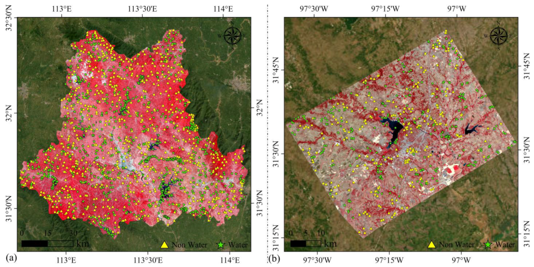
To further validate the generalization ability of transfer learning, two regions including Suizhou City in Hubei Province, China (31°19′–32°26′N, 112°43′–113°46′E) and McAllen County in Texas, USA (31°15′–31°50′N, 96°45′–97°45′W) have been selected for validation as shown in Figure 2. Suizhou City (Figure 2a) has an area of approximately 9636 km2, while McAllen County (Figure 2b) has an area of approximately 2745 km2. Both regions contain various types of surface water bodies, including small and medium reservoirs, artificial lakes, ponds, and narrow rivers. We obtained multiple validation sample points in two regions using visual interpretation (Figure 2). Specifically, we obtained 1601 sample points in Suizhou City (766 non-water sample points and 835 water sample points) and 530 sample points in McLean County (265 non-water sample points and 265 water sample points). All the models have been assessed using sample points through manual interpretation.

2.2. Data Sources

2.2.1. Sentinel-2 Data

Sentinel-2 imagery and corresponding water masks were employed for pre-training deep learning segmentation models. The publicly available S1S2-Water dataset, which is a global reference dataset specifically designed for training and evaluating convolutional neural networks in water body semantic segmentation [36], was adopted to pre-train the deep learning models. Since the original dataset incorporates both Sentinel-1 SAR and Sentinel-2 optical imagery, only the Sentinel-2 components were retained for this study to maintain spectral consistency with optical PlanetScope data. The S1S2-Water dataset comprises 65 Sentinel-2 scenes, each containing six spectral bands (Blue: 490 nm, Green: 560 nm, Red: 665 nm, NIR: 842 nm, SWIR1: 1610 nm, SWIR2: 2190 nm) accompanied by the corresponding binary water masks (0: non-water, 1: water). Each image contains 10,980 × 10,980 pixels at 10 m spatial resolution.

2.2.2. PlanetScope Data

The PlanetScope constellation, consisting of more than 180 Dove satellites, provides daily global coverage at 3 m spatial resolution. The original Dove satellites captured only four spectral bands (Red, Green, Blue, and Near-Infrared), and the upgraded SuperDove constellation deployed since August 2021 added four additional bands (Green I, Red Edge, Yellow, and Coastal Blue). As shown in Table 1, our analysis is limited to the four original bands (RGB-NIR) to ensure temporal consistency across the five-year study period and compatibility with established small water body mapping methodologies [6,7]. This approach aligns with previous research, which demonstrate superior performance of four-band 10 m Sentinel-2 imagery compared with incorporating 20 m resolution bands for small water body detection [37,38].
In this study, a total of 26 PlanetScope images were used. These images were acquired at different seasons, which enables us to assess the deep learning model to map small water bodies with various phenological features. The detailed information about the used PlanetScope is in Appendix A Table A1.

2.3. Dataset Pre-Processing

For the Sentinel-2 dataset from S1S2-Water dataset used for pre-training, all 65 scenes and corresponding water masks were partitioned into non-overlapping 256 × 256 pixel patches. The patches were quantitatively stratified into 1%-interval bins according to water coverage percentage, followed by proportional allocation into training (70%) and validation (30%) subsets through stratified random sampling. This preprocessing generated a Sentinel-2 training dataset comprising 53,112 training patches and 22,767 validation patches.
For the PlanetScope dataset for fine-tuning, the PlanetScope imagery was manually annotated to binary water masks. Since water boundary may be blurred in the PlanetScope image, the manual annotation is performed by incorporating higher-resolution (1 m) Google Earth imagery that is temporally adjacent to PlanetScope. After annotation, both the PlanetScope images and corresponding water masks were systematically partitioned into non-overlapping 256 × 256 pixel patches. The final dataset contains 5648 patches (4356 for training and validation, 1292 for testing).

2.4. Model Architecture and Training

2.4.1. Deep Learning Network for Small Water Body Segmentation

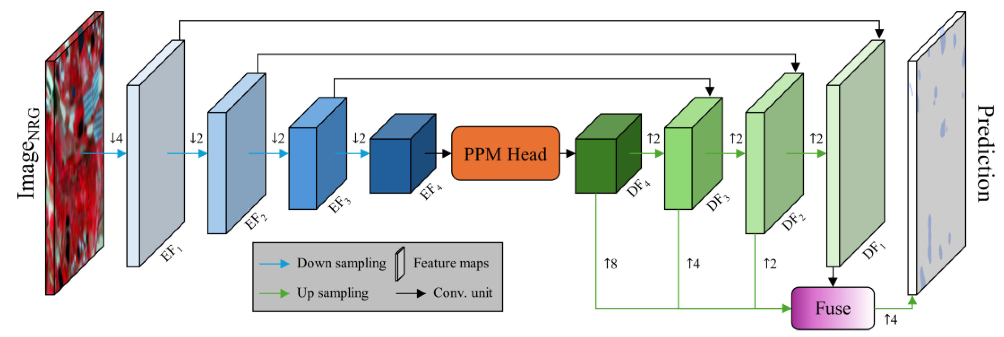
As illustrated in Figure 3, the UperNet with an encoder–decoder semantic segmentation architecture has been explored in this study. The model extracts multi-scale encoder features (EFi, i = 1, 2, 3, 4) from the input image through the backbone network and inputs them into the decoder to obtain multi-scale decoder features (DFi, i = 1, 2, 3, 4). Among these, the EF4 features are refined by a pyramid pooling module (PPM) to generate DF4. A Feature Pyramid Network (FPN) subsequently fuses these hierarchical features and produces DF3, DF2, and DF1. All feature maps (excluding DF1) are upsampled to 1/4 resolution of the input image, concatenated, and fed into the segmentation classifier for pixel-wise prediction.
This study evaluates eight foundational network architectures, including VMamba, MambaOut, CoAtNet, MaxViT, Swin Transformer (SwinT), ConvNeXt, ResNet, and Xception, which represent state-of-the-art paradigms in visual backbone design. These architectures have been extensively adopted in image segmentation tasks, including surface water mapping, due to their hierarchical feature extraction capabilities. To ensure architectural consistency, all eight backbone networks were implemented with four-stage encoder frameworks. This standardized four-stage configuration enables systematic comparison of their feature learning characteristics while maintaining compatibility with dense prediction tasks. The detailed encoder structures, including channel dimension configurations and block arrangements, are visualized in Figure 4.
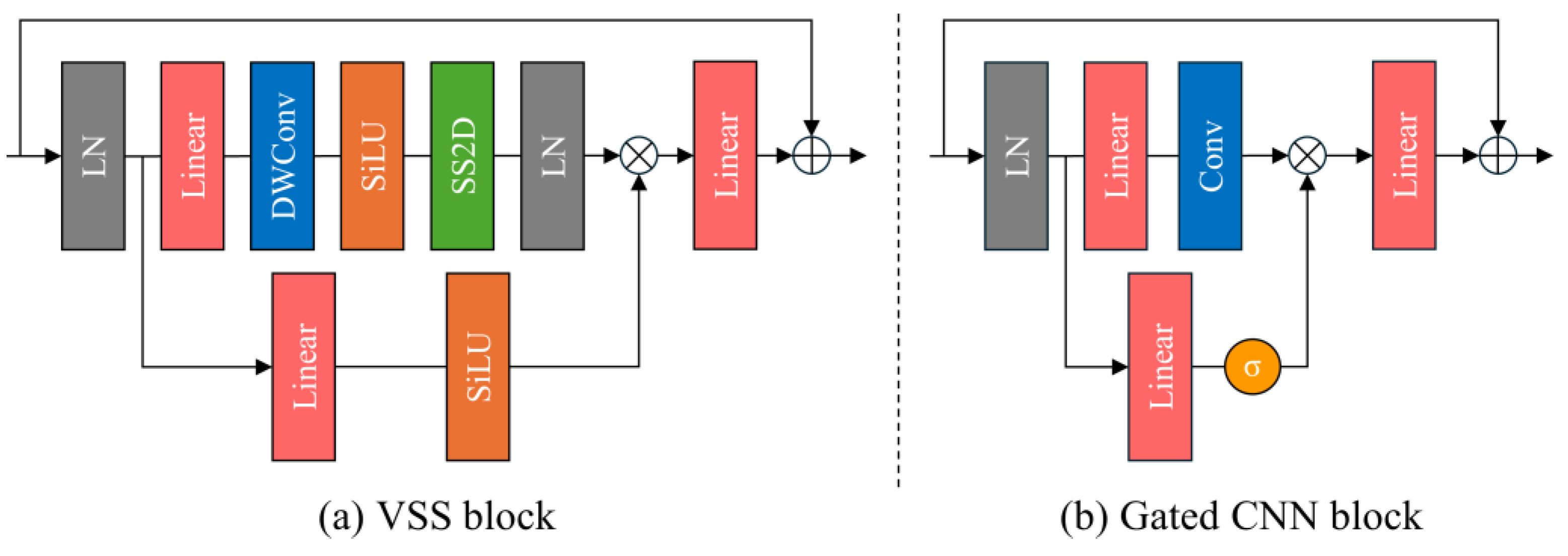
VMamba, proposed in 2024, aims to develop a novel backbone network that combines the low complexity of CNNs with the strong fitting capacity of Vision Transformers. Its core innovation is the Visual State-Space (VSS) module, which extends the Mamba model (originally designed for 1D natural language processing) to handle 2D image data in computer vision. By introducing the Cross-Scan Module (CSM) and the 2D Selective Scanning method (SS2D), VMamba addresses the directional sensitivity issue of State-Space Models (SSMs) in visual tasks while preserving global perception and dynamic feature selection capabilities. Through architectural optimizations of the VSS block, VMamba maintains linear computational complexity alongside excellent representational power, demonstrating significant potential as a next-generation visual backbone. The structural details are presented in Figure 5a and Appendix B Table A2.
MambaOut, proposed in 2024, investigates the necessity of SSMs for visual tasks, demonstrating that Mamba’s applicability requires both long-sequence and auto-regressive characteristics. It replaces SSMs with stacked Gated CNN blocks and further simplifies the model architecture. While MambaOut outperforms visual Mamba models on the ImageNet classification task, its performance on long-sequence tasks like detection and segmentation is comparable yet inconclusive against visual Mamba variants, warranting further validation. The structural details are presented in Figure 5b and Appendix B Table A2.
CoAtNet, proposed in 2021, is a hybrid vision architecture that synergistically combines CNNs and Transformers, leveraging the strong generalization capacity of CNN with the global receptive field of Transformer. The framework unifies mobile inverted residual convolutions (MBConv) with relative position self-attention (Rel-SA) modules through a cohesive design. This design preserves the local inductive bias inherent to CNNs while incorporating the global receptive field of Transformers, enabling an effective balance between efficiency and performance across diverse data scales. The structural details are presented in Figure 6a,b and Appendix B Table A3.
MaxViT, a hybrid architecture algorithm, was proposed in 2022. This algorithm introduces a multi-axis self-attention (Max-SA) mechanism based on CoAtNet, capturing fine-grained features within local regions through block-wise computation and enabling global feature interaction across regions through an expansion strategy. This approach expands the receptive field while minimizing computational complexity. The structural details are presented in Figure 6a–c and Appendix B Table A3.
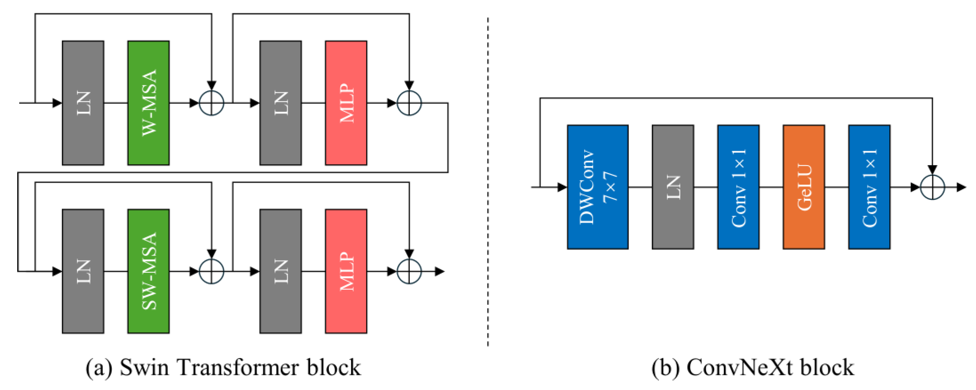
Swin Transformer, proposed in 2021, is a vision model based on the Vision Transformer architecture. It employs a shifted window mechanism: the image is partitioned into non-overlapping fixed-size windows where self-attention is computed locally (W-MSA), and cross-window communication is achieved via periodic window shifts (SW-MSA). Additionally, it adopts a hierarchical structure where image patches are progressively merged, facilitating multi-scale feature extraction and enhancing global structure modeling capabilities. The structural details are presented in Figure 7a and Appendix B Table A4.
ConvNeXt, proposed in 2022, is a pure CNN architecture designed following Swin Transformer principles. Building upon the traditional ResNet, it replaces standard convolutions with 7 × 7 depth-wise convolutions to enlarge the receptive field. Batch Normalization (BN) and ReLU activations are substituted with Layer Normalization (LN) and GELU, respectively. The introduction of a hierarchical design enhances performance while maintaining the inherent efficiency of CNNs. The structural details are presented in Figure 7b and Appendix B Table A4.
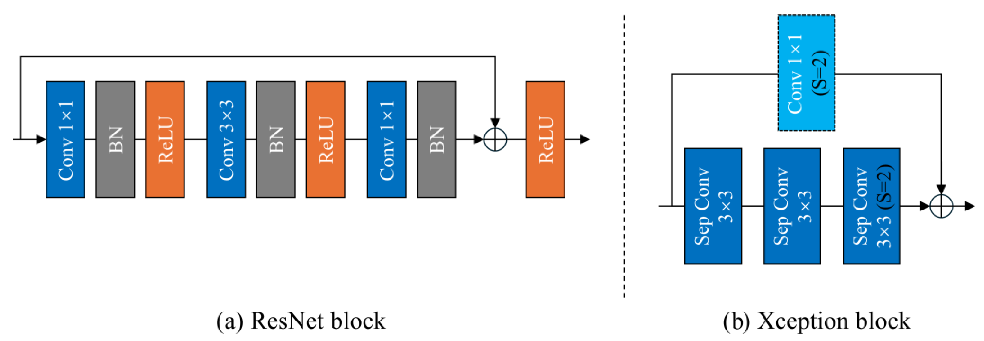
ResNet, proposed in 2015, is a classic CNN architecture. Its core innovation is the residual learning framework, where inputs are directly added (via skip connections) to the outputs of convolutional layers. This effectively mitigates the vanishing gradient problem and model degradation in deep network training. The structural details are presented in Figure 8a and Appendix B Table A5.
Xception, proposed in 2016 and later refined in DeepLabV3+, significantly reduces parameters while maintaining performance through the use of depth-wise separable convolutions. The structural details are presented in Figure 8b and Appendix B Table A5.

2.4.2. Model Training Strategy and Comparison

This study evaluated transfer learning feasibility for small water body mapping through three approaches: (1) baseline models trained exclusively on Sentinel-2 data (denoted as “pre-training”); (2) fine-tuning models where Sentinel-2 pre-trained weights were further optimized using limited PlanetScope data (denoted as “fine-tuning”); and (3) from-scratch training on PlanetScope data alone (denoted as “from-scratch training”).
To mitigate spectral discrepancies between Sentinel-2 and PlanetScope imagery, the fine-tuning strategy employed a reduced learning rate (10% of global rate) for backbone layers while maintaining standard rates for task-specific heads. All experiments were implemented in PyTorch 2.8.0 dev. Input data were standardized using the mean and standard deviation values of their respective datasets. Data augmentations included random geometric transformations (horizontal/vertical flips, 90° rotations), and random rectangular occlusions (number [ 1 , 3 ] , size [ 13 , 25 ] ) were applied to the training samples. During the model training phase, considering that a single accuracy evaluation metric has certain limitations [39], we obtained a ‘combine score’ (Table 2) by simply weighing and combining multiple metrics to comprehensively evaluate the performance of models.
Since the PalnetScope image dataset used for direct training and transfer learning is relatively small, we adopted a five-fold cross-validation [40] scheme to obtain robust prediction results. This reduces the impact of model training errors, training sample imbalance, and model architecture on the prediction results. All models use the same data partitioning, and a fixed random seed is used for each training run. All models maintained consistency in training hyperparameters (including optimizer selection, learning rate, batch size, and data augmentation strategies) and were not individually tuned.
In this study, all computational experiments were performed on a workstation equipped with an Intel Core i7-14700K CPU and an NVIDIA GeForce RTX 5080 GPU. All deep learning models were built using PyTorch 2.8.0 dev, with a CUDA version of 12.8. Comprehensive training configurations for the three strategies are summarized in Table 2.

2.5. Accuracy Assessment

The segmentation performance was quantitatively assessed using five metrics derived from the confusion matrix, including True Positives (TP) for correctly classified water pixels, True Negatives (TN) for accurately identified non-water regions, False Positives (FP) representing non-water misclassified as water, and False Negatives (FN) indicating water omission. Based on these metrics, we computed Producer’s Accuracy (PA), quantifying omission errors; User’s Accuracy (UA), measuring commission errors; Overall Accuracy (OA), reflecting global classification correctness, along with F1 Score and Mean Intersection over Union (MIoU), providing class-imbalance-resistant spatial and probabilistic assessments.
PA = TP TP + FN
UA = TP TP + FP
OA = TP + TN TP + FP + TN + FN
F 1 = 2 TP 2 TP + FP + FN
MIoU = TP TN + FP + FN + TN TP + FP + FN 2 TP + FP + FN TN + FP + FN

3. Results

3.1. Five-Fold Cross-Validation of Fine-Tuning Strategies and From-Scratch Training Strategies Using PlanetScope

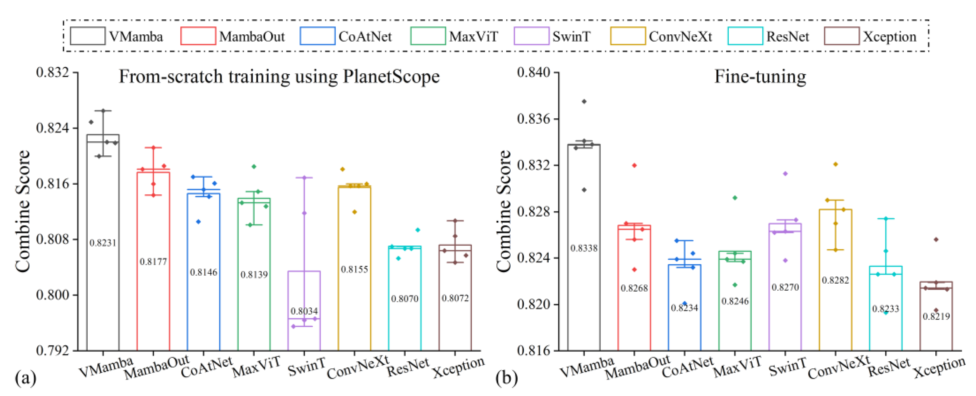
Since the focus of this paper is on assessing strategies for training with limited PlanetScope imagery, the pre-training strategy using a large number of Sentinel-2 images has not been evaluated with five-fold cross-validation in this section. The five-fold cross-validation (Table 3, Figure 9) highlights that VMamba achieved the highest accuracy in both from-scratch strategies and fine-tuning, using ‘combine score’ in Table 2 as the accuracy metric. In the from-scratch training in Figure 9a, SwinT generated the lowest accuracy and the highest variance. This is mainly because high accuracy of SwinT is usually based on a relatively large number of training data, while the training data used in the from-scratch training (approximately one thousand patches) is relatively small and is limited to training a robust model. In the accuracy plots from fine-tuning in Figure 9b, VMamba achieved the highest mean combined scores (0.8338), which increased about 0.56% and 1.19% compared with MambaOut and Xception. Compared to models based on hybrid architectures, VMamba also increased accuracy (e.g., VMamba increased 1.04% compared with CoAtNet), showing that it is robust when only a limited number of training data is available for fine-tuning. In addition, VMamba generated a standard deviation of 0.0024 in the five-fold cross-validation experiment in the fine-tuning results in Figure 9b, showing its robustness in mapping small water bodies with changed training samples. This superiority in VMamba stems from its SSM-based design, which captures long-range dependencies in multispectral data while maintaining computational efficiency.

3.2. Comparison Between Pre-Training and Fine-Tuning

Table 4 shows the quantitative metrics from pre-training and fine-tuning. Pre-learning from Sentinel-2 imagery yielded OA ranging from 0.92 to 0.96 across all networks. In particular, Xception demonstrated higher accuracy (OA = 0.9528, F1 = 0.76.68, MIoU = 0.7938) followed closely by ResNet (OA = 0.9528, F1 = 0.7533, MIoU = 0.7848). VMamba and MambaOut showed relatively lower accuracy (0.01 decrease in OA) compared to CNN-based models. For the pre-training strategy, the UA values were about 0.15 lower than the PA values, indicating large commission errors when applying pre-training models directly to PlanetScope imagery without fine-tuning. These findings reveal domain shifts between Sentinel-2 and PlanetScope data.
Fine-tuning with limited PlanetScope imagery yielded enhanced accuracy across all evaluated networks in Table 4. Compared with pre-training, fine-tuning increased OA by 0.0376 (VMamba), 0.0349 (MambaOut), 0.0291 (CoAtNet), 0.0480 (MaxViT), 0.0416 (SwinT), 0.0348 (ConvNeXt), 0.0226 (ResNet), and 0.0203 (Xception), respectively. The fine-tuning strategy enhanced both UA and PA for all eight networks compared with pre-training, demonstrating its effectiveness in decreasing both omission and commission errors. ResNet achieved the highest PA (0.9184) but the lowest UA (0.8017) among all models, while VMamba had a better-balanced PA (0.9117) and UA (0.8288). VMamba generated the highest OA (0.9781), F1 (0.8661), and MIoU (0.8710). The increased accuracies from fine-tuning compared with pre-training validate the effectiveness of the proposed two-stage transfer learning framework, which leverages large-scale Sentinel-2 pre-training followed by targeted PlanetScope fine-tuning, in small water body mapping.
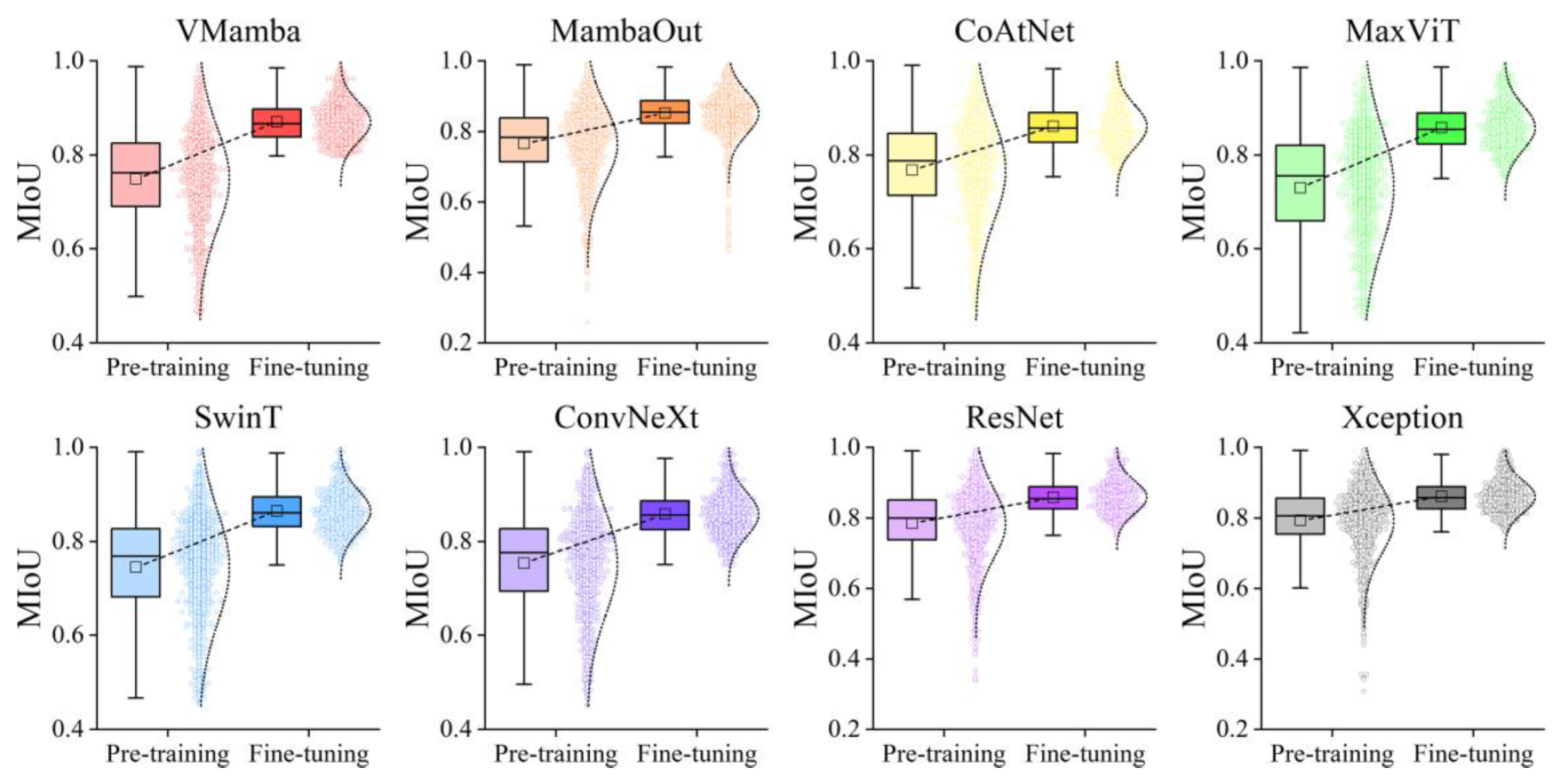
Figure 10 visualizes the corresponding MIoU accuracies for all 1292 testing patches before and after fine-tuning using boxplots. The results demonstrate that all fine-tuning models achieved an average MIoU exceeding 0.80. The changes in median MIoU values suggest that fine-tuning effectively reduced the occurrence of low-accuracy samples. MaxViT exhibited the most substantial improvement before and after fine-tuning (0.1277 increase in average MIoU). In addition, the boxplot analysis reveals a more concentrated MIoU sample distribution after fine-tuning, indicating enhanced robustness in surface water mapping accuracy.
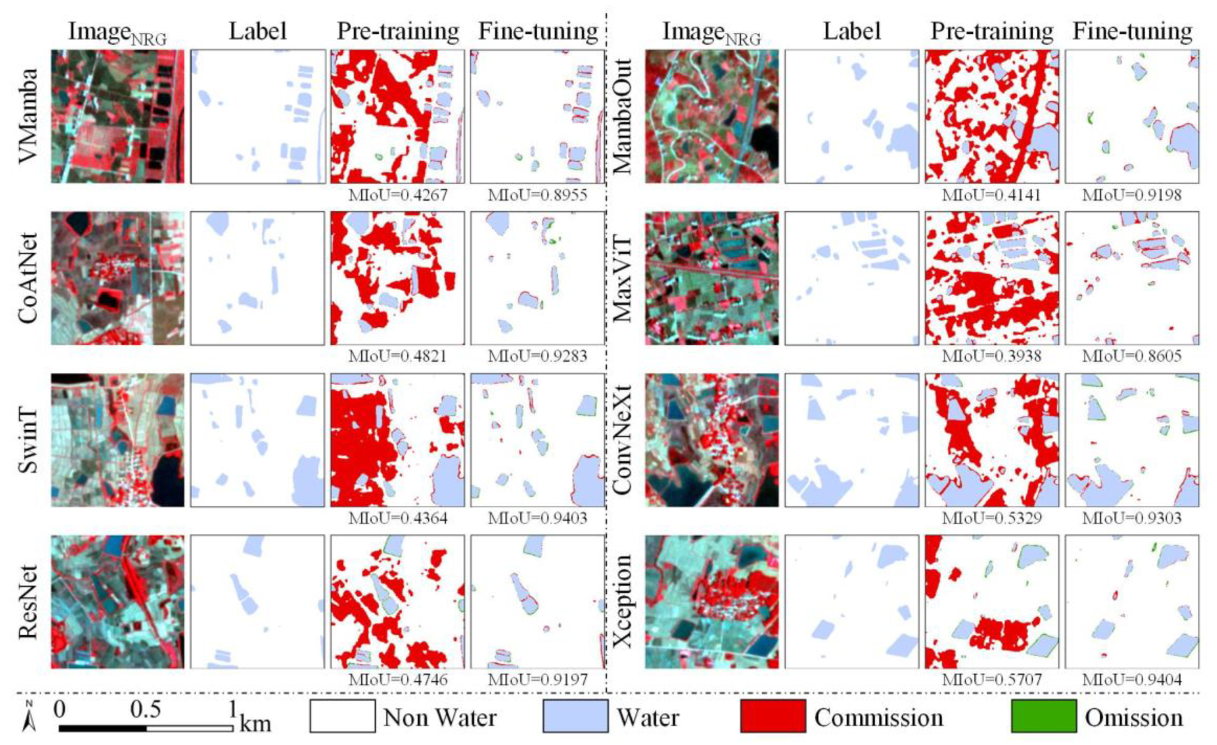
Figure 11 illustrates the comparative water mapping results generated by eight backbone networks from pre-training and fine-tuning across representative regions. Visual analysis reveals that all pre-training networks before fine-tuning produced substantial commission errors (highlighted in red). This is obvious by the misclassification of dark-colored vegetated areas and light-blue built-up regions in PlanetScope imagery as water bodies. From the fine-tuning, all networks reduced commission errors. This is consistent with the quantitative improvements shown in Table 3, where UA increased from 0.60 to 0.70 to over 0.80. For the water maps generated from fine-tuning, omission and commission errors were mainly located along small water body boundaries. Quantitatively, fine-tuning improved MIoU across all architectures, with VMamba showing an increase from 0.4267 to 0.8955 and CoAtNet increasing from 0.5329 to 0.9303. This finding reveals the effectiveness of the fine-tuning approach in transfer learning from Sentinel-2 to PlanetScope.
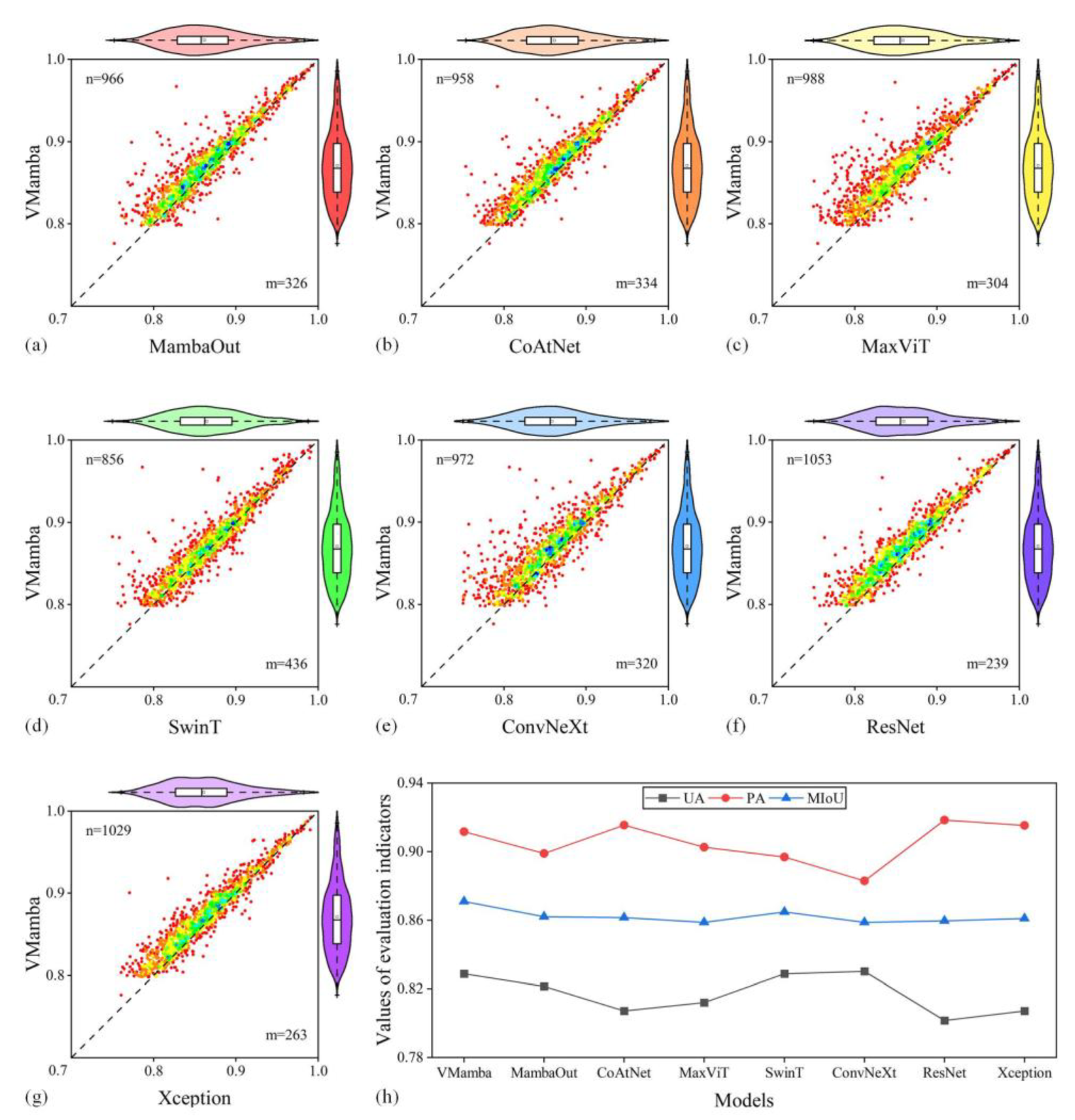
Figure 12 presents a comparative analysis of MIoU performance between VMamba and seven other backbone networks after fine-tuning. The scatter plot distributions demonstrated that the majority of sample points lie above the 1:1 reference line, showing that VMamba achieved higher MIoU compared to other models. Quantitative evaluation also reveals VMamba (denoted as ‘n’ in Figure 12) outperformed competing architectures (denoted as ‘m’) in a greater number of test patches. VMamba exhibited the highest n/m ratios compared with ResNet (Figure 12f, n/m = 4.41). VMamba also achieved a high n/m ratio compared with the Transformer-based SwinT network (Figure 12d), showing VMamba predicted higher MIoU values in more test patches.
The violin plot analysis in Figure 12 demonstrates that VMamba exhibits a more concentrated MIoU distribution characterized by both a higher median value and superior lower quartile performance relative to comparative models, confirming its enhanced robustness in water segmentation tasks. While the distributions of UA and PA across the eight networks (Figure 12h) reveal that VMamba does not achieve the highest individual values for these metrics, its highest MIoU demonstrates an optimal trade-off between omission and commission errors.
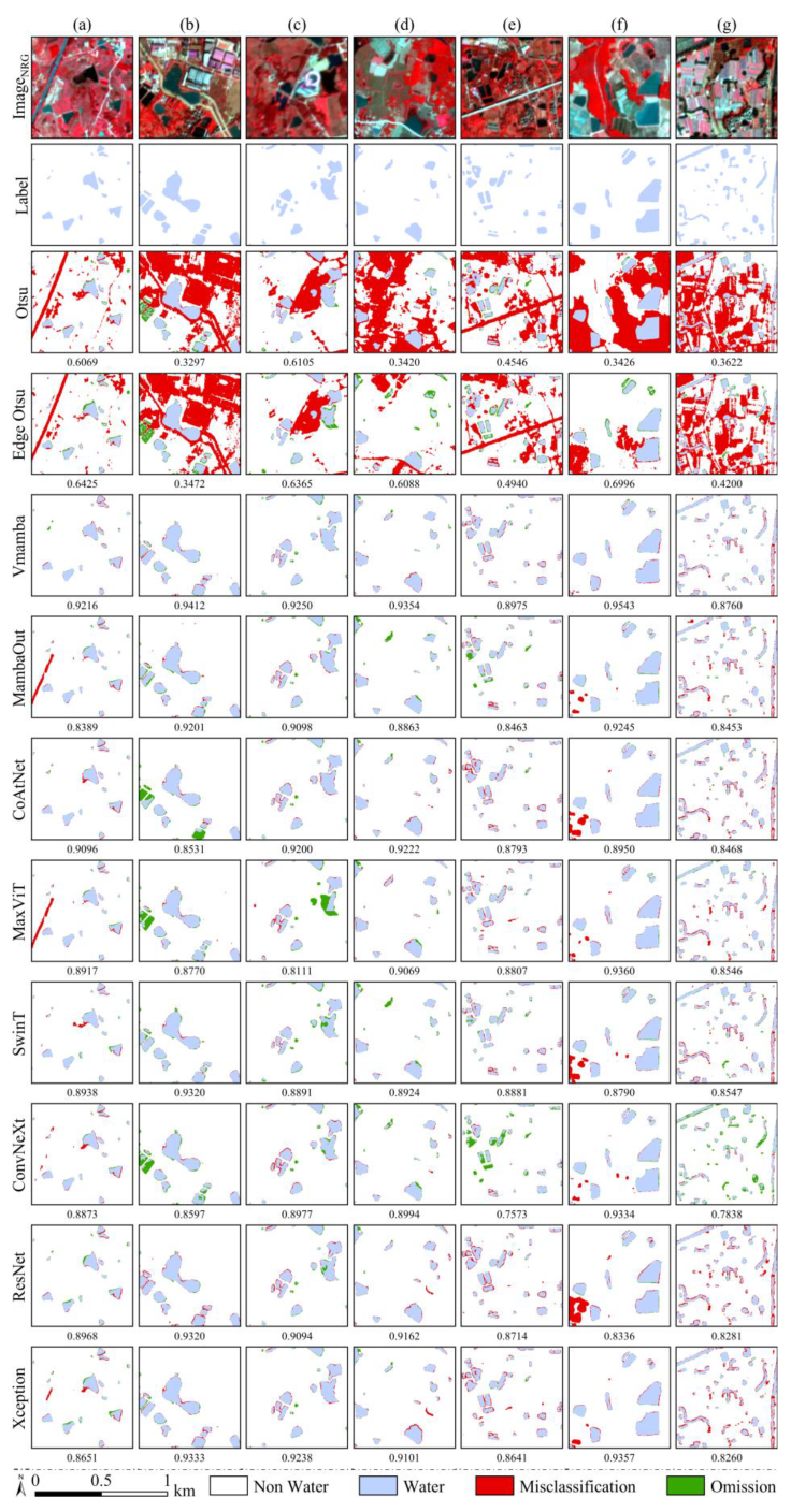
Figure 13 presents a comparative analysis of surface water segmentation performance across fine-tuned networks and two state-of-the-art automated methods (Otsu [41] and Edge-Otsu [42] algorithms). The conventional Otsu and Edge-Otsu methods exhibited obvious commission errors, primarily attributable to the misclassification of dark-toned non-water features (e.g., roads and bare soil) as water bodies (red highlights). In contrast, all deep learning architectures demonstrated a substantial decrease in commission errors. This finding reveals their superior capacity for extracting high-level semantic features from remote sensing imagery. Among the networks, VMamba generated surface water maps with minimal commission and omission errors, especially for small water bodies. VMamba correctly classified road segments that were misidentified as water by MambaOut and Xception in Figure 13a. VMamba detected small ponds that were not mapped by CoAtNet, MaxViT, and ConvNeXt in Figure 13b. Moreover, VMamba better mapped the shape of water bodies compared with SwinT in Figure 13d and decreased commission errors observed in ResNet and Xception outputs in Figure 13f. Quantitative analysis shows VMamba generated the highest MIoU across all test regions.

3.3. Comparison Fine-Tuning with From-Scratch Training Using PlanetScope

This section compares the fine-tuning model with from-scratch training using PlanetScope, to assess which method is better when only a limited number of training samples are available. Table 5 demonstrates that fine-tuning consistently outperforms from-scratch training. This is mainly due to the extensive data coverage of Sentinel-2 imagery used for pre-training the deep learning model, which enables the model to learn general spatial and spectral characteristics of surface water bodies. All networks trained from scratch (Table 5) were found to outperform those pre-trained exclusively on Sentinel-2 data without fine-tuning (Table 4). This finding reveals an obvious domain gap between these sensors while simultaneously underscoring the critical role of fine-tuning for PlanetScope small water body detection.
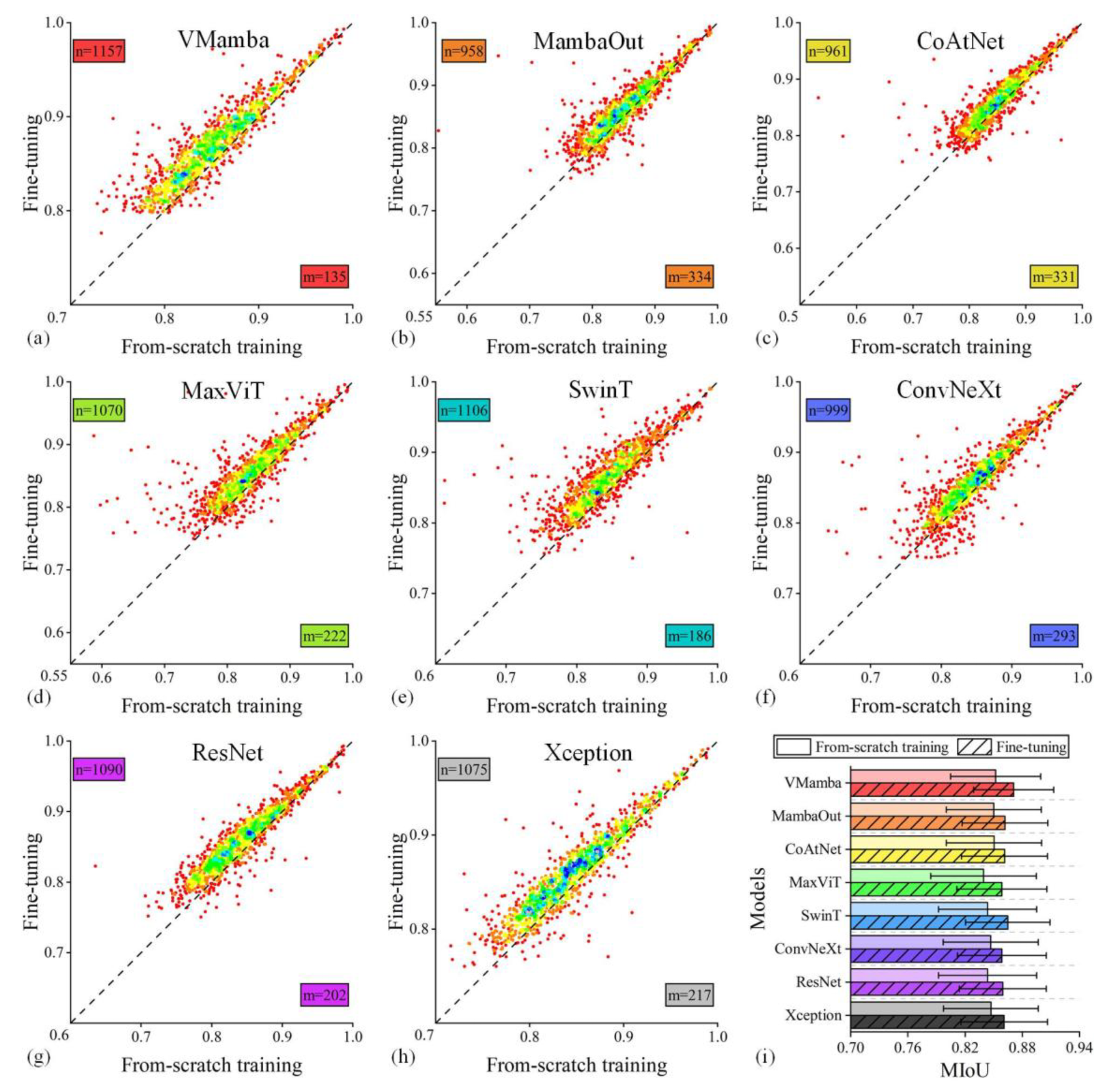
Figure 14 presents a comprehensive comparison of MIoU distributions between fine-tuning versus from-scratch training using PlanetScope. The scatter plot in Figure 14a–h analysis reveals most points were above the 1:1 line, quantitatively demonstrating that fine-tuning outperformed from-scratch training in most test patches. The quantitative analysis in Figure 14i showed significantly higher mean MIoU values for fine-tuning models, and VMamba exhibited both the highest mean accuracy and lowest standard deviation. This finding demonstrates the robustness of VMamba in small water body mapping. It is also found that VMamba achieves the highest n/m ratio of 8.57 in Figure 14a. These results show the effectiveness of cross-sensor transfer learning and architectural advantages of VMamba in PlanetScope water mapping applications.
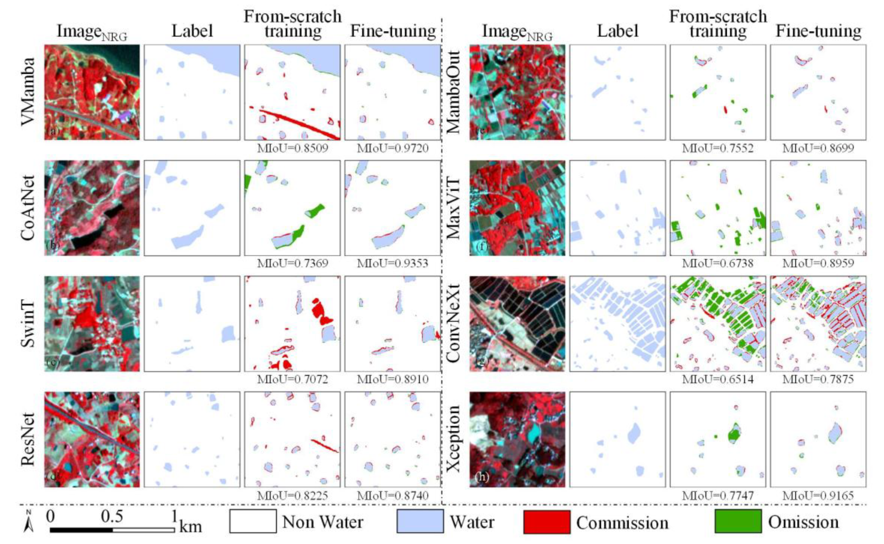
Figure 15 presents a comparative visualization of water mapping results between fine-tuning and from-scratch training using PlanetScope across multiple test sites. Results reveal that from-scratch training exhibits significantly higher commission errors, with commission from roads (Figure 15a,d) and dense vegetation (Figure 15c) indicated by red pixels. Fine-tuning networks reduced the commission errors in red pixels while simultaneously reducing the omission errors in green pixels (Figure 15b,e–h). In addition, the fine-tuning approach better delineates the boundary of small water features in Figure 15d,h with improved MIoU, and the result validated the efficacy of this transfer learning strategy when there is limited availability of high-resolution PlanetScope training samples.

3.4. Validating the Generalization Capability of Transfer Learning Models Across Diverse Networks

In this study, all eight deep learning models have been used to map surface water. The fine-tuning strategy was considered since it outperformed the pre-training and from-scratch training strategies as shown in the aforementioned tests. The unsupervised Otsu and Edge-Otsu were also compared. In addition, the classic machine learning model of Random Forest has been compared. Random Forest is an ensemble learning method that constructs multiple decision trees using bootstrap aggregation and random feature selection during training, then combines predictions through majority voting (classification) to improve accuracy and robustness. The training sample point data was obtained through manual visual interpretation and included different types of surface water bodies and non-water bodies to ensure sample diversity and, as far as possible, to ensure that the sample points were evenly distributed throughout the study area. In particular, 1300 sample points were identified in Suizhou City (650 non-water body samples and 650 water body samples), and 530 sample points were identified (295 non-water body samples and 295 water body samples) in McLean County.
Table 6 presents a comparative analysis of accuracy metrics from different methods. In general, the unsupervised methods of Otsu and Edge-Otsu generated the lowest OA and F1, since they did not explore any prior information about the surface water bodies. The shallow machine learning Random Forest increased the OA and F1 values compared with the unsupervised methods. In contrast, all the deep learning models generated higher OA and F1 than the unsupervised methods and the Random Forest classifier in Table 6. In particular, all models that were enhanced via transfer learning exhibited OA and F1 scores exceeding 0.92 and PA scores above 0.89. This finding shows that the shallow machine learning model may be overfit, while the deep learning model can better extract the deep semantic information inherent in surface water bodies. Among the various deep learning models, VMamba generated the highest OA (0.9825), F1 score (0.9832), and PA (0.9820), showing its effectiveness in surface water body extraction.
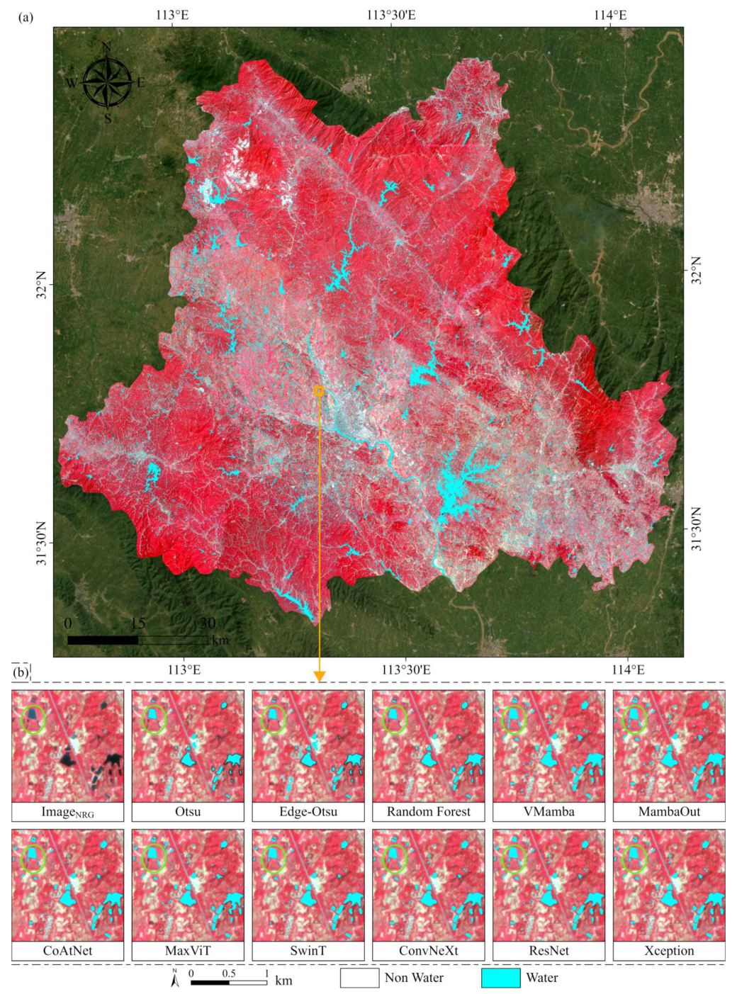
Figure 16a illustrates the surface water distribution map in Suizhou City generated by VMamba, which generated the highest OA and F1. VMamba has detected diverse water bodies, including rivers, medium-to-small reservoirs, and numerous small-scale water features. Figure 16b shows zoomed-in regions of Figure 16a obtained using different methods. The threshold-based methods and shallow machine learning approaches failed to detect many small water bodies, such as those highlighted with green ellipses in Figure 16b. Among the various deep learning models, CoAtNet, MaxViT, SwinT, and Xception only detected part of the small water bodies highlighted with green ellipses, while VMamba and other models better mapped these small water bodies. This result underscores the advantages of transfer learning in large-scale surface water mapping, particularly for PlanetScope-derived data, where the hierarchical architecture of VMamba and cross-scale feature decoding makes it robust in mapping various small water bodies.
Table 7 presents the accuracy metrics from multiple models in the McLennan study area. Consistent with findings in the Suizhou region, VMamba achieved the highest OA (0.9604), F1 score (0.9616), and PA (0.9887). All deep learning models outperformed traditional unsupervised classifications (Otsu and Edge-Otsu) and shallow machine learning of Random Forest. This cross-regional consistency highlights the adaptability and robustness of transfer learning frameworks and underscores the VMamba architecture’s generalizability in surface water mapping using high-resolution PlanetScope imagery.
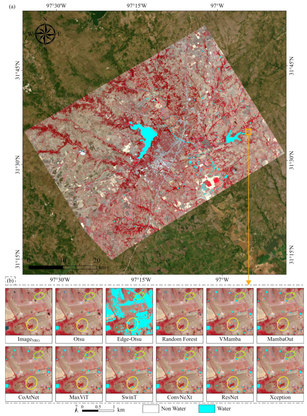
Figure 17a shows the surface water map of the McLennan study area generated by VMamba. Small and medium reservoirs and small ponds have been detected by VMamba. As shown in the zoom areas of Figure 17b, Edge-Otsu has misclassified many non-water bodies as surface water. Otsu and Random Forest failed to detect many small ponds, such as those highlighted with green and yellow ellipses in Figure 17b. In contrast, all the deep learning models have detected most of the ponds in the zoom areas. Among the various deep learning methods, MambaOut and MaxViT failed to map or only mapped part of the ponds highlighted with green and yellow ellipses, while VMamba and other deep learning models better mapped these ponds. This finding also highlights the generalization capacity of deep learning with transfer learning in large-scale surface water mapping and the advantage of the VMamba architecture.

4. Discussion

4.1. Impact of the Pre-Trained Data in Transfer Learning

This study employs the S1S2-water dataset, comprising Sentinel-2 imagery and corresponding water masks, for network pre-training before PlanetScope fine-tuning. The stratified random sampling design of the dataset ensures comprehensive coverage across diverse climatic zones, atmospheric conditions, and land cover types. This sampling strategy provides distinct advantages for pre-training deep learning networks to extract robust water body features across various geographical contexts. While the dataset excels in capturing large water bodies, its representation of small water features remains limited. In addition, S1S2-water dataset has collected abundant samples for flood mapping, which incorporate many inundated region samples. Thus, using S1S2-water dataset in pre-training may result in relatively large commission errors when mapping dark objects such as shadows and dense vegetations as water bodies. Besides S1S2-water dataset, other Sentinel-2 water masks, such as in [43], could also be applied to pre-train the networks. In addition, open-access land cover products also contain a water category that is helpful in pre-training. For instance, the Dynamic World, which is a globally stratified sampled training dataset [44], contains more than twenty thousand patches and could also be explored to pre-train the network for constructing a robust model.

4.2. The Impact of Model Hyperparameters

In this work, we isolate the impact of network architecture on small-water-body classification by keeping all other training variables constant. Specifically, we use the same hyperparameter set for all eight models (Table 2). While a dedicated hyperparameter search for each architecture might improve absolute accuracy, it would introduce an additional experimental variable. This would make direct comparisons of architectural effectiveness difficult.
Although we did not perform a formal hyperparameter search for each model (beyond a few informal pilot trials to prevent failures), prior research shows that relative performance rankings are usually robust when hyperparameters fall within a reasonable range. For example, Bengio [45] notes that sensible defaults often achieve near-optimal performance for many deep models. Similarly, Choi et al. [46] show that once optimizers and models are tuned to avoid obvious misconfigurations, their relative performance stabilizes. Novello et al. [47] further support this using sensitivity analysis, demonstrating that fine-tuning within an appropriate range rarely changes the comparative ranking of architectures.
We acknowledge that dedicated tuning per model (e.g., grid search or Bayesian optimization) could further improve absolute accuracies and potentially change the ranking. However, such extensive searches are beyond the scope of this study, whose primary goal is a controlled architectural comparison. They would also require a prohibitively large computational budget. Therefore, we leave comprehensive hyperparameter optimization as a promising direction for future work.

4.3. The Impact of Model Complexity

Experimental results demonstrate that VMamba consistently outperforms popular backbones (MambaOut, CoAtNet, MaxViT, Swin Transformer, ConvNeXt, and ResNet) in mapping small water bodies. This success stems from two key design innovations: the SS2D module, which enlarges the receptive field with minimal computational cost and sharpens edge and region detail, and the cross-shaped spatial mixing (CSM) module with a four-directional 2D scanning path, which captures multi-directional continuity more effectively than standard convolutions or local window attention. By contrast, MambaOut does not include a State-Space Model (SSM) module, which limits its global modeling capabilities. CNNs are hampered by narrow receptive fields, and Transformers lack adaptive feature selection for complex boundaries. In terms of complexity (Table 8), VMamba uses linear-cost state-space mechanisms to model large-scale features but carries 35.23 M parameters (134.49 MB) and requires about 40 min per ten epochs. Meanwhile, lighter networks like MambaOut (25.91 M parameters, 36 min/10 epochs) run faster, and the depth-wise separable convolutions of Xception still incur 28.40 GFLOPs. Swin Transformer and ConvNeXt train in around 30 min but remain limited by local receptive fields. These results highlight the inevitable trade-off between expressive power, computational load, and operational speed in backbone design.

4.4. Limitation and Future Works

Although the proposed transfer learning framework exhibits great potential for small water body mapping in PlanetScope imagery with a limited number of training samples, several limitations should be noted. First, although the networks maintain a proper balance between omission and commission errors during small water body detection, precisely delineating complex-shaped water bodies, particularly those with intricate shapes and heterogeneous surrounding landscapes, remains challenging. For instance, ConvNext tended to misclassify dense aquaculture areas, produced oversmoothed shapes, and struggled to distinguish individual ponds or precisely delineate their boundaries when multiple small water bodies are clustered closely together. To address these issues, future studies could explore developing advanced attention mechanisms [29], incorporating domain knowledge [12], or implementing class imbalance mitigation strategies [19]. Second, while this study utilized four 10 m resolution Sentinel-2 bands for network pre-training, the potential of 20 m spectral bands (particularly the coastal blue band at 443 nm, which is spectrally consistent between Sentinel-2 and PlanetScope) remains unexplored for cross-sensor transfer learning applications. Lastly, our current framework does not incorporate topographic information (e.g., DEM-derived features) in Sentinel-2-based water detection, which may potentially enhance water mapping accuracy. With recent advancements in global DEM products, future research should investigate DEM integration to further improve transfer learning performance for small water body mapping, particularly in mountainous and hilly regions.

5. Conclusions

This study presents a comprehensive investigation of cross-sensor transfer learning methodologies for small water body detection, evaluating eight state-of-the-art deep learning architectures (including CNN, Transformer, and novel VMamba) through a systematic knowledge transfer framework from Sentinel-2 to PlanetScope imagery. As deep learning represents a data-driven methodology, the accuracy of small water body detection from high spatiotemporal resolution PlanetScope data depends critically on the availability of training samples with water masks. Given the relatively short operational history of PlanetScope and the labor-intensive nature of manual water mask delineation from its imagery, pre-training networks using existing open-source Sentinel-2 water mapping datasets show significant potential for improving mapping accuracy while minimizing human intervention. Our methodology leverages open-source Sentinel-2 water datasets for pre-training, followed by fine-tuning with selected PlanetScope samples (1292 patches). The transfer learning achieved an MIoU of 0.87, an overall accuracy of 0.97, and an F1-score of 0.86. Fine-tuning improved these metrics compared with pre-training by over 0.10 while simultaneously decreasing both commission and omission errors. Fine-tuning demonstrates particular efficacy in decreasing both commission errors from roads and vegetation and omission errors in small ponds and narrow channels compared to pre-training. Architectural comparison reveals the superior performance of VMamba across various accuracy metrics, attributable to its unique ability to capture long-range spatial dependencies while maintaining computational efficiency. Spatial validation across regions of 9636 km2 and 2745 km2 confirms the method’s robustness and generalization capacity. This research establishes that a strategic combination of large-scale Sentinel-2 pre-training (incorporating seasonal variations and global water feature diversity) with targeted PlanetScope fine-tuning (requiring only a small number of samples compared with traditional training data) can overcome the fundamental data limitations in high-resolution water mapping while reducing manual annotation requirements.

Author Contributions

Conceptualization, Y.L. and X.L. (Xiaodong Li); Methodology, Y.L.; Software, Y.L.; Validation, Y.W. and X.L. (Xiang Li); Investigation, Y.L.; Writing—original draft, Y.L. and P.Z.; Writing—review & editing, Y.Z. and X.L. (Xiaodong Li); Supervision, X.L. (Xiaodong Li); Project administration, X.L. (Xiaodong Li); Funding acquisition, Y.Z. and X.L. (Xiaodong Li). All authors have read and agreed to the published version of the manuscript.

Funding

This work was supported by the Joint Funds of the National Natural Science Foundation of China (U24A20587), 2025 Central Government Guidance Fund for Local Science and Technology Development (Directed Commissioning Program for Platform Infrastructure), Department of Science and Technology of Hubei province (ZYYDJCC202500015), the Natural Science Foundation of China (42271400), and Young Top-notch Talent Cultivation Program of Hubei Province.

Institutional Review Board Statement

Not applicable.

Informed Consent Statement

Not applicable.

Data Availability Statement

Data will be made available on request. The code is available at the following link (https://github.com/YuyangLi001/rs_3731045, accessed on 24 July 2025).

Acknowledgments

The authors thank the Planet Labs Company and Google Company for providing images for research analysis.

Conflicts of Interest

The authors declare no conflicts of interest.

Appendix A

Table A1. Information about the used PlanetScope images.
IDImage Acquisition TimesImage Location
(Upper Left Corner)
Image Size in Pixels
(Height, Width)
126 May 2017117.68°N, 32.18°E3973 × 4804
217 July 2017111.97°N, 29.86°E4018 × 4160
323 July 2017111.96°N, 32.02°E4695 × 4367
42 January 2018109.50°N, 23.08°E5073 × 3855
512 January 2018119.07°N, 32.02°E5198 × 3958
628 March 2018115.17°N, 31.91°E5207 × 3871
71 April 2018116.21°N, 28.15°E1754 × 6995
88 April 2018116.54°N, 30.72°E3733 × 4193
97 June 2018112.62°N, 30.97°E6668 × 5668
1028 June 2018113.28°N, 30.17°E2864 × 3762
118 September 2018114.47°N, 31.08°E5667 × 4054
1214 March 2019111.52°N, 30.69°E4002 × 3668
136 April 2019111.48°N, 32.57°E3668 × 4001
1424 August 2019111.81°N, 29.94°E3335 × 3334
1520 March 2020112.25°N, 31.79°E2431 × 2611
1626 April 2020111.51°N, 30.56°E4961 × 4146
1720 May 2020119.11°N, 31.55°E5423 × 3196
1811 October 2020116.79°N, 31.71°E4257 × 4471
1924 October 2020118.90°N, 32.53°E3423 × 3220
2010 November 2020117.84°N, 31.37°E6616 × 3300
2112 November 2020117.31°N, 32.50°E8691 × 4745
2230 November 2020117.54°N, 31.22°E5145 × 3255
237 May 2021117.87°N, 31.00°E5223 × 4104
2426 September 2021118.23°N, 32.52°E5251 × 3879
2526 May 2017118.97°N, 32.00°E4862 × 3882
2617 July 2017113.75°N, 31.18°E3723 × 5249

Appendix B

Table A2. Structures of VMamba and MambaOut.
Layer NameOutput SizeVMambaMambaOut
Stem64 × 64 Conv   3 × 3 ,   4 48 ,   stride   2 Conv   3 × 3 ,   48 96 ,   stride   2
Stage164 × 64 Linear   96 2 × 96 DWConv   3 × 3 ,   2 × 96 SS 2 D ,   dim   2 × 96 Linear   2 × 96 96 × 2 Linear   96 256 ,   160 ,   96 DWConv   7 × 7 ,   96 Cat ( 160 ,   96 ) 256 256 Linear   256 96 × 3
Stage232 × 32 Conv   3 × 3 ,   96 192 ,   stride   2
Linear   192 2 × 192 DWConv   3 × 3 ,   2 × 192 SS 2 D ,   dim   2 × 192 Linear   2 × 192 192 × 2 Linear   192 512 ,   320 ,   192 DWConv   7 × 7 ,   192 Cat ( 320 ,   192 ) 512 512 Linear   512 192 × 3
Stage316 × 16 Conv   3 × 3 ,   192 384 ,   stride   2
Linear   384 2 × 384 DWConv   3 × 3 ,   2 × 384 SS 2 D ,   dim   2 × 384 Linear   2 × 384 384 × 6 Linear   384 1024 ,   640 ,   384 DWConv   7 × 7 ,   384 Cat ( 640 ,   384 ) 1024 1024 Linear   1024 384 × 9
Stage48 × 8 Conv   3 × 3 ,   384 768 ,   stride   2
Linear   768 2 × 768 DWConv   3 × 3 ,   2 × 768 SS 2 D ,   dim   2 × 768 Linear   2 × 768 768 × 2 Linear   576 1536 ,   960 ,   576 DWConv   7 × 7 ,   576 Cat ( 960 ,   576 ) 1536 1536 Linear   1536 576 × 3
Table A3. Structures of CoAtNet and MaxViT.
Layer NameOutput SizeCoAtNetMaxViT
Stem128 × 128 Conv   3 × 3 ,   4 32 ,   stride   2 Conv   3 × 3 ,   32 64
Stage164 × 64 AvgPool   2 × 2 ,   stride   2
    Conv   1 × 1 ,   64 96 Conv   1 × 1 ,   96 384 DWConv   3 × 3 ,   384 SE ,   384 96 384 Conv   1 × 1 ,   384 96 × 2 DWConv   7 × 7 ,   64 MLP ,   64 256 64 BlockAttn , 64 MLP ,   64 256 64 GridAttn , 64 MLP ,   64 256 64 × 2
Stage232 × 32 AvgPool   2 × 2 ,   stride   2
Conv   1 × 1 ,   96 192
Conv   1 × 1 ,   192 768 DWConv   3 × 3 ,   768 SE ,   768 192 768 Conv   1 × 1 ,   768 192 × 3
Conv   1 × 1 ,   64 128
DWConv   7 × 7 ,   128 MLP ,   128 512 128 BlockAttn , 128 MLP ,   128 512 128 GridAttn , 128 MLP ,   128 512 128 × 2
Stage316 × 16 AvgPool   2 × 2 ,   stride   2
Conv   1 × 1 ,   192 384
Rel-Attn ,   384   Conv   1 × 1 ,   384 1536 Conv   1 × 1 ,   1536 384 × 7
Conv   1 × 1 ,   128 256
DWConv   7 × 7 ,   256 MLP ,   256 1024 256 BlockAttn , 256 MLP ,   256 1024 256 GridAttn , 256 MLP ,   256 1024 256 × 5
Stage48 × 8 AvgPool   2 × 2 ,   stride   2
Conv   1 × 1 ,   384 768
Rel-Attn ,   768   Conv   1 × 1 ,   768 3072 Conv   1 × 1 ,   3072 768 × 2
Conv   1 × 1 ,   256 512
DWConv   7 × 7 ,   512 MLP ,   512 2048 512 BlockAttn , 512 MLP ,   512 2048 512 GridAttn , 512 MLP ,   512 2048 512 × 2
Table A4. Structures of Swin Transformer and ConvNeXt.
Layer NameOutput SizeSwin TransformerConvNeXt
Stem64 × 64 Conv   4 × 4 ,   4 96 ,   stride   4
Stage1 W-MSA   7 × 7 ,   96 ,   head   3 MLP ,   96 384 96 × 2 DWConv   7 × 7 ,   96 Conv   1 × 1 ,   96 384 Conv   1 × 1 ,   384 96 × 3
Stage232 × 32 PixelUnshuffle   ,   96 384 Linear ,   384 192 Conv   2 × 2 ,   96 192 ,   stride   2
W - MSA   7 × 7 ,   192 ,   head   6 MLP ,   192 768 192 × 2 DWConv   7 × 7 ,   192 Conv   1 × 1 ,   192 768 Conv   1 × 1 ,   768 192 × 3
Stage316 × 16 PixelUnshuffle   ,   192 768 Linear ,   768 384 Conv   2 × 2 ,   192 384 ,   stride   2
W-MSA   7 × 7 ,   384 ,   head   12 MLP ,   384 1536 384 × 6 DWConv   7 × 7 ,   384 Conv   1 × 1 ,   384 1536 Conv   1 × 1 ,   1536 384 × 9
Stage48 × 8 PixelUnshuffle ,   384 1536 Linear ,   1536 768 Conv   2 × 2 ,   384 768 ,   stride   2
W-MSA   7 × 7 ,   768 ,   head   24 MLP ,   768 3072 768 × 2 DWConv   7 × 7 ,   768 Conv   1 × 1 ,   768 3072 Conv   1 × 1 ,   3072 768 × 3
Table A5. Structures of ResNet and Xception.
Layer NameOutput SizeResNetXception
Stem128 × 128 Conv   3 × 3 ,   4 32 ,   stride   2 Conv   3 × 3 ,   32 Conv   3 × 3 ,   32 64 Conv   3 × 3 ,   4 32 ,   stride   2 Conv   3 × 3 ,   32 64
Stage164 × 64 MaxPool   3 × 3 ,   stride   2 SepConv   3 × 3 ,   64 128 SepConv   3 × 3 ,   128 SepConv   3 × 3 ,   128 ,   stride   2
Conv   1 × 1 , 64   Conv   3 × 3 ,   64 Conv   1 × 1 ,   64 256 × 3 SepConv   3 × 3 ,   128 256 SepConv   3 × 3 ,   256 SepConv   3 × 3 ,   256 ,   stride   2
Stage232 × 32 AvgPool   2 × 2 ,   stride   2 SepConv   3 × 3 ,   256 736 SepConv   3 × 3 ,   736 SepConv   3 × 3 ,   736 ,   stride   2
Conv   1 × 1 ,   128   Conv   3 × 3 ,   128 Conv   1 × 1 ,   128 512 × 4
Stage316 × 16 AvgPool   2 × 2 ,   stride   2 SepConv   3 × 3 ,   736 SepConv   3 × 3 ,   736 SepConv   3 × 3 ,   736 × 16
Conv   1 × 1 ,   256   Conv   3 × 3 ,   256 Conv   1 × 1 ,   256 1024 × 6
Stage48 × 8 AvgPool   2 × 2 ,   stride   2 SepConv   3 × 3 ,   736 1024 SepConv   3 × 3 ,   1024 SepConv   3 × 3 ,   1024 ,   stride   2
Conv   1 × 1 ,   512   Conv   3 × 3 ,   512 Conv   1 × 1 ,   512 2048 × 3 SepConv   3 × 3 ,   1024 1536 SepConv   3 × 3 ,   1536 SepConv   3 × 3 ,   1536 2048

References

  1. Li, L.; Long, D.; Wang, Y.; Woolway, R.I. Global Dominance of Seasonality in Shaping Lake-Surface-Extent Dynamics. Nature 2025, 642, 361–368. [Google Scholar] [CrossRef]
  2. Pekel, J.-F.; Cottam, A.; Gorelick, N.; Belward, A.S. High-Resolution Mapping of Global Surface Water and Its Long-Term Changes. Nature 2016, 540, 418–422. [Google Scholar] [CrossRef] [PubMed]
  3. Yang, X.; Zhao, S.; Qin, X.; Zhao, N.; Liang, L. Mapping of Urban Surface Water Bodies from Sentinel-2 MSI Imagery at 10 m Resolution via NDWI-Based Image Sharpening. Remote Sens. 2017, 9, 596. [Google Scholar] [CrossRef]
  4. Yang, X.; Qin, Q.; Yésou, H.; Ledauphin, T.; Koehl, M.; Grussenmeyer, P.; Zhu, Z. Monthly Estimation of the Surface Water Extent in France at a 10-m Resolution Using Sentinel-2 Data. Remote Sens. Environ. 2020, 244, 111803. [Google Scholar] [CrossRef]
  5. Freitas, P.; Vieira, G.; Canário, J.; Folhas, D.; Vincent, W.F. Identification of a Threshold Minimum Area for Reflectance Retrieval from Thermokarst Lakes and Ponds Using Full-Pixel Data from Sentinel-2. Remote Sens. 2019, 11, 657. [Google Scholar] [CrossRef]
  6. Mullen, A.L.; Watts, J.D.; Rogers, B.M.; Carroll, M.L.; Elder, C.D.; Noomah, J.; Williams, Z.; Caraballo-Vega, J.A.; Bredder, A.; Rickenbaugh, E.; et al. Using High-Resolution Satellite Imagery and Deep Learning to Track Dynamic Seasonality in Small Water Bodies. Geophys. Res. Lett. 2023, 50, e2022GL102327. [Google Scholar] [CrossRef]
  7. Valman, S.J.; Boyd, D.S.; Carbonneau, P.E.; Johnson, M.F.; Dugdale, S.J. An AI Approach to Operationalise Global Daily PlanetScope Satellite Imagery for River Water Masking. Remote Sens. Environ. 2024, 301, 113932. [Google Scholar] [CrossRef]
  8. Flores, J.A.; Gleason, C.J.; Brinkerhoff, C.B.; Harlan, M.E.; Lummus, M.M.; Stearns, L.A.; Feng, D. Mapping Proglacial Headwater Streams in High Mountain Asia Using PlanetScope Imagery. Remote Sens. Environ. 2024, 306, 114124. [Google Scholar] [CrossRef]
  9. Perin, V.; Roy, S.; Kington, J.; Harris, T.; Tulbure, M.G.; Stone, N.; Barsballe, T.; Reba, M.; Yaeger, M.A. Monitoring Small Water Bodies Using High Spatial and Temporal Resolution Analysis Ready Datasets. Remote Sens. 2021, 13, 5176. [Google Scholar] [CrossRef]
  10. Perin, V.; Tulbure, M.G.; Gaines, M.D.; Reba, M.L.; Yaeger, M.A. A Multi-Sensor Satellite Imagery Approach to Monitor on-Farm Reservoirs. Remote Sens. Environ. 2022, 270, 112796. [Google Scholar] [CrossRef]
  11. Chanda, M.; Hossain, A.K.M.A. Application of PlanetScope Imagery for Flood Mapping: A Case Study in South Chickamauga Creek, Chattanooga, Tennessee. Remote Sens. 2024, 16, 4437. [Google Scholar] [CrossRef]
  12. Zhou, P.; Li, X.; Zhang, Y.; Wang, Y.; Li, Y.; Li, X.; Zhou, C.; Shen, L.; Du, Y. Domain-Knowledge-Guided Multisource Fusion Network for Small Water Bodies Mapping Using PlanetScope Multispectral and Google Earth RGB Images. IEEE J. Sel. Top. Appl. Earth Obs. Remote Sens. 2025, 18, 2541–2562. [Google Scholar] [CrossRef]
  13. Freitas, P.; Vieira, G.; Canário, J.; Vincent, W.F.; Pina, P.; Mora, C. A Trained Mask R-CNN Model over PlanetScope Imagery for Very-High Resolution Surface Water Mapping in Boreal Forest-Tundra. Remote Sens. Environ. 2024, 304, 114047. [Google Scholar] [CrossRef]
  14. Kang, J.; Guan, H.; Ma, L.; Wang, L.; Xu, Z.; Li, J. WaterFormer: A Coupled Transformer and CNN Network for Waterbody Detection in Optical Remotely-Sensed Imagery. ISPRS J. Photogramm. Remote Sens. 2023, 206, 222–241. [Google Scholar] [CrossRef]
  15. Ma, D.; Jiang, L.; Li, J.; Shi, Y. Water Index and Swin Transformer Ensemble (WISTE) for Water Body Extraction from Multispectral Remote Sensing Images. GIScience Remote Sens. 2023, 60, 2251704. [Google Scholar] [CrossRef]
  16. Liu, Z.; Lin, Y.; Cao, Y.; Hu, H.; Wei, Y.; Zhang, Z.; Lin, S.; Guo, B. Swin Transformer: Hierarchical Vision Transformer Using Shifted Windows. In Proceedings of the 2021 IEEE/CVF International Conference on Computer Vision (ICCV), Montreal, BC, Canada, 1–17 October 2021; pp. 9992–10002. [Google Scholar]
  17. Dai, Z.; Liu, H.; Le, Q.V.; Tan, M. CoAtNet: Marrying Convolution and Attention for All Data Sizes. Available online: https://arxiv.org/abs/2106.04803 (accessed on 5 August 2025).
  18. Liu, Y.; Tian, Y.; Zhao, Y.; Yu, H.; Xie, L.; Wang, Y.; Ye, Q.; Jiao, J.; Liu, Y. VMamba: Visual State Space Model. Adv. Neural Inf. Process. Syst. 2024, 37, 103031–103063. [Google Scholar]
  19. Zhou, P.; Foody, G.; Zhang, Y.; Wang, Y.; Wang, X.; Li, S.; Shen, L.; Du, Y.; Li, X. Using an Area-Weighted Loss Function to Address Class Imbalance in Deep Learning-Based Mapping of Small Water Bodies in a Low-Latitude Region. Remote Sens. 2025, 17, 1868. [Google Scholar] [CrossRef]
  20. Ding, N.; Qin, Y.; Yang, G.; Wei, F.; Yang, Z.; Su, Y.; Hu, S.; Chen, Y.; Chan, C.-M.; Chen, W.; et al. Parameter-Efficient Fine-Tuning of Large-Scale Pre-Trained Language Models. Nat. Mach. Intell. 2023, 5, 220–235. [Google Scholar] [CrossRef]
  21. Liu, Z.; Xu, Y.; Xu, Y.; Qian, Q.; Li, H.; Ji, X.; Chan, A.; Jin, R. Improved Fine-Tuning by Better Leveraging Pre-Training Data. Adv. Neural Inf. Process. Syst. 2022, 35, 32568–32581. [Google Scholar]
  22. Martins, V.S.; Roy, D.P.; Huang, H.; Boschetti, L.; Zhang, H.K.; Yan, L. Deep Learning High Resolution Burned Area Mapping by Transfer Learning from Landsat-8 to PlanetScope. Remote Sens. Environ. 2022, 280, 113203. [Google Scholar] [CrossRef]
  23. Anand, A.; Imasu, R.; Dhaka, S.; Patra, P.K. Domain Adaptation and Fine-Tuning of a Deep Learning Segmentation Model of Small Agricultural Burn Area Detection Using Hi-Resolution Sentinel-2 Observations: A Case Study of Punjab, India. Remote Sens. 2025, 17, 974. [Google Scholar] [CrossRef]
  24. Wang, Z.; Gao, X.; Zhang, Y. HA-Net: A Lake Water Body Extraction Network Based on Hybrid-Scale Attention and Transfer Learning. Remote Sens. 2021, 13, 4121. [Google Scholar] [CrossRef]
  25. Wu, P.; Fu, J.; Yi, X.; Wang, G.; Mo, L.; Maponde, B.T.; Liang, H.; Tao, C.; Ge, W.; Jiang, T.; et al. Research on Water Extraction from High Resolution Remote Sensing Images Based on Deep Learning. Front. Remote Sens. 2023, 4, 1283615. [Google Scholar] [CrossRef]
  26. Pickens, A.H.; Hansen, M.C.; Hancher, M.; Stehman, S.V.; Tyukavina, A.; Potapov, P.; Marroquin, B.; Sherani, Z. Mapping and Sampling to Characterize Global Inland Water Dynamics from 1999 to 2018 with Full Landsat Time-Series. Remote Sens. Environ. 2020, 243, 111792. [Google Scholar] [CrossRef]
  27. Pi, X.; Luo, Q.; Feng, L.; Xu, Y.; Tang, J.; Liang, X.; Ma, E.; Cheng, R.; Fensholt, R.; Brandt, M.; et al. Mapping Global Lake Dynamics Reveals the Emerging Roles of Small Lakes. Nat. Commun. 2022, 13, 5777. [Google Scholar] [CrossRef] [PubMed]
  28. Lv, M.; Wu, S.; Ma, M.; Huang, P.; Wen, Z.; Chen, J. Small Water Bodies in China: Spatial Distribution and Influencing Factors. Sci. China Earth Sci. 2022, 65, 1431–1448. [Google Scholar] [CrossRef]
  29. Jiang, C.; Zhang, H.; Wang, C.; Ge, J.; Wu, F. Water Surface Mapping from Sentinel-1 Imagery Based on Attention-UNet3+: A Case Study of Poyang Lake Region. Remote Sens. 2022, 14, 4708. [Google Scholar] [CrossRef]
  30. Isikdogan, F.; Bovik, A.C.; Passalacqua, P. Surface Water Mapping by Deep Learning. IEEE J. Sel. Top. Appl. Earth Obs. Remote Sens. 2017, 10, 4909–4918. [Google Scholar] [CrossRef]
  31. Yu, W.; Wang, X. MambaOut: Do We Really Need Mamba for Vision? Available online: https://arxiv.org/abs/2405.07992 (accessed on 5 August 2025).
  32. Tu, Z.; Talebi, H.; Zhang, H.; Yang, F.; Milanfar, P.; Bovik, A.; Li, Y. MaxViT: Multi-Axis Vision Transformer. In Lecture Notes in Computer Science; Springer Nature: Cham, Switzerland, 2022; pp. 459–479. [Google Scholar]
  33. Liu, Z.; Mao, H.; Wu, C.-Y.; Feichtenhofer, C.; Darrell, T.; Xie, S. A ConvNet for the 2020s. In Proceedings of the 2022 IEEE/CVF Conference on Computer Vision and Pattern Recognition (CVPR), New Orleans, LA, USA, 18–24 June 2022. [Google Scholar]
  34. He, K.; Zhang, X.; Ren, S.; Sun, J. Deep Residual Learning for Image Recognition. In Proceedings of the 2016 IEEE Conference on Computer Vision and Pattern Recognition (CVPR), Vegas, NV, USA, 7–30 June 2016; pp. 770–778. [Google Scholar]
  35. Chen, L.-C.; Zhu, Y.; Papandreou, G.; Schroff, F.; Adam, H. Encoder-Decoder with Atrous Separable Convolution for Semantic Image Segmentation. In Lecture Notes in Computer Science; Springer International Publishing: Cham, Switzerland, 2018; pp. 833–851. [Google Scholar]
  36. Wieland, M.; Fichtner, F.; Martinis, S.; Groth, S.; Krullikowski, C.; Plank, S.; Motagh, M. S1S2-Water: A Global Dataset for Semantic Segmentation of Water Bodies from Sentinel- 1 and Sentinel-2 Satellite Images. IEEE J. Sel. Top. Appl. Earth Obs. Remote Sens. 2024, 17, 1084–1099. [Google Scholar] [CrossRef]
  37. Liu, D.; Zhu, X.; Holgerson, M.; Bansal, S.; Xu, X. Inventorying Ponds Through Novel Size-Adaptive Object Mapping Using Sentinel-1/2 Time Series. Remote Sens. Environ. 2024, 315, 114484. [Google Scholar] [CrossRef]
  38. Zhou, P.; Li, X.; Foody, G.M.; Boyd, D.S.; Wang, X.; Ling, F.; Zhang, Y.; Wang, Y.; Du, Y. Deep Feature and Domain Knowledge Fusion Network for Mapping Surface Water Bodies by Fusing Google Earth RGB and Sentinel-2 Images. IEEE Geosci. Remote Sens. Lett. 2023, 20, 1–5. [Google Scholar] [CrossRef]
  39. Reinke, A.; Tizabi, M.D.; Sudre, C.H.; Eisenmann, M.; Rädsch, T.; Baumgartner, M.; Acion, L.; Antonelli, M.; Arbel, T.; Bakas, S.; et al. Common Limitations of Image Processing Metrics: A Picture Story. arXiv 2021, arXiv:2104.05642. [Google Scholar] [CrossRef]
  40. Ait tchakoucht, T.; Elkari, B.; Chaibi, Y.; Kousksou, T. Random Forest with Feature Selection and K-Fold Cross Validation for Predicting the Electrical and Thermal Efficiencies of Air Based Photovoltaic-Thermal Systems. Energy Rep. 2024, 12, 988–999. [Google Scholar] [CrossRef]
  41. Otsu, N. A Threshold Selection Method from Gray-Level Histograms. IEEE Trans. Syst. Man Cybern. 1979, 9, 62–66. [Google Scholar] [CrossRef]
  42. Kolli, M.K.; Opp, C.; Karthe, D.; Pradhan, B. Automatic Extraction of Large-Scale Aquaculture Encroachment Areas Using Canny Edge Otsu Algorithm in Google Earth Engine—The Case Study of Kolleru Lake, South India. Geocarto Int. 2022, 37, 11173–11189. [Google Scholar] [CrossRef]
  43. Luo, X.; Tong, X.; Hu, Z. An Applicable and Automatic Method for Earth Surface Water Mapping Based on Multispectral Images. Int. J. Appl. Earth Obs. Geoinf. 2021, 103, 102472. [Google Scholar] [CrossRef]
  44. Brown, C.F.; Brumby, S.P.; Guzder-Williams, B.; Birch, T.; Hyde, S.B.; Mazzariello, J.; Czerwinski, W.; Pasquarella, V.J.; Haertel, R.; Ilyushchenko, S.; et al. Dynamic World, Near Real-Time Global 10 m Land Use Land Cover Mapping. Sci. Data 2022, 9, 251. [Google Scholar] [CrossRef]
  45. Bengio, Y. Practical Recommendations for Gradient-Based Training of Deep Architectures. In Lecture Notes in Computer Science; Springer: Berlin/Heidelberg, Germany, 2012; pp. 437–478. [Google Scholar]
  46. Choi, D.; Shallue, C.J.; Nado, Z.; Lee, J.; Maddison, C.J.; Dahl, G.E. On Empirical Comparisons of Optimizers for Deep Learning. arXiv 1910, arXiv:1910.05446. [Google Scholar] [CrossRef]
  47. Novello, P.; Poëtte, G.; Lugato, D.; Congedo, P.M. Goal-Oriented Sensitivity Analysis of Hyperparameters in Deep Learning. J. Sci. Comput. 2023, 94, 45. [Google Scholar] [CrossRef]
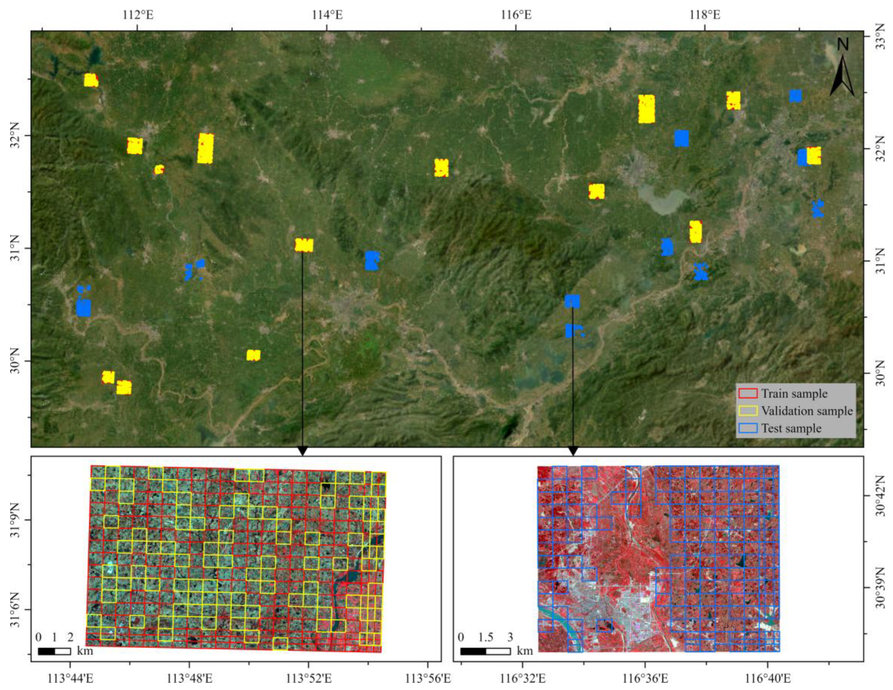
Figure 1. The distribution of image patches used in this study. The training (red) and validation (yellow) patches are illustrated in the lower left corner, and the validation (blue) patch is illustrated in the lower right corner.
Remotesensing 17 02738 g001
Figure 2. False color PlanetScope image in the study area and distribution of validation sample points. (a) Suizhou City; (b) McAllen County.
Remotesensing 17 02738 g002
Figure 3. Structure of the UperNet algorithm. ↓n indicates downsampling by a factor of n, ↑n indicates upsampling by a factor of n (n = 2, 4, 8).
Remotesensing 17 02738 g003
Figure 4. Overview of encoder of UperNet.
Remotesensing 17 02738 g004
Figure 5. Overview of the basic module of the VMamba and MambaOut algorithms. (a) The Visual State-Space (VSS) block in VMamba; (b) the Gated CNN block in MambaOut.
Remotesensing 17 02738 g005
Figure 6. Overview of the basic module of the CoAtNet and MaxViT algorithms. (a) The MBConv block in CoAtNet and MaxViT; (b) the Transformer block in CoAtNet and MaxViT; (c) the multi-axis strategy in MaxViT.
Remotesensing 17 02738 g006
Figure 7. Overview of the basic module of the Swin Transformer and ConvNeXt algorithms.
Remotesensing 17 02738 g007
Figure 8. Overview of the basic module of the ResNet and Xception algorithms.
Remotesensing 17 02738 g008
Figure 9. Five-fold cross-validation of two strategies. (a) Combined scores of each model when trained from scratch on the PlanetScope dataset; (b) Combined scores of each model after fine-tuning based on pre-trained weights on the PlanetScope dataset.
Remotesensing 17 02738 g009
Figure 10. Comparison of MIoU of different networks from pre-training and fine-tuning. The lighter-colored areas represent the accuracy results of pre-training, while the darker-colored areas represent the results of fine-tuning.
Remotesensing 17 02738 g010
Figure 11. Visualization of classification results for typical regions of different methods from pre-training and fine-tuning.
Remotesensing 17 02738 g011
Figure 12. Differences in MIoUs between VMamba and other networks from fine-tuning using the 1292 test patches. In (ag), the points located above the 1:1 line (y > x) show VMamba outperformed the competitors; otherwise, points located below the 1:1 line (y < x) show competitors generated higher MIoU. The darker box plots represent the accuracy results of VMamba, while the lighter box plots represent the accuracy results of other algorithms. n indicates the number of test patches where VMamba outperformed the competitors, and m indicates the number of test patches where the competitors outperformed VMamba. In (h), the three accuracy evaluation metrics for different models are shown.
Remotesensing 17 02738 g012
Figure 13. Comparison of different water mapping results from fine-tuning. In (ag), the classification results of eight algorithms are shown when there are differences in the distribution range and size of water bodies.
Remotesensing 17 02738 g013
Figure 14. Comparison of MIoU between fine-tuning and from-scratch training using PlanetScope, using the 1292 test patches. (a) VMamba (red), (b) MambaOut (orange), (c) CoAtNet (yellow), (d) MaxViT (green), (e) SwinT (cyan), (f) ConvNeXt (blue), (g) ResNet (purple), (h) Xception (gray). The points located above the 1:1 line (y > x) show fine-tuning outperformed from-scratch training; otherwise, points located below the 1:1 line (y < x) show from-scratch training generated higher MIoU. n indicates the number of test patches where fine-tuning outperformed the from-scratch training, and m indicates the number of test patches where from-scratch training outperformed fine-tuning. (i) Differences in MIoU across models under the two strategies.
Remotesensing 17 02738 g014
Figure 15. Comparison of water mapping results between fine-tuning and from-scratch training using PlanetScope.
Remotesensing 17 02738 g015
Figure 16. (a) Surface water mapping result from VMamba in Suizhou, China and (b) the resultant surface water maps in the zoom area from various methods. The green circle indicates areas where there are significant differences between the classification results of the algorithms.
Remotesensing 17 02738 g016
Figure 17. (a) Surface water mapping result from VMamba in McLennan County, Texas, USA and (b) the resultant surface water maps in the zoom area from various methods. The green and yellow circles indicate areas where there are significant differences between the classification results of the algorithms.
Remotesensing 17 02738 g017
Table 1. Comparison of spectral bands between PlanetScope and Sentinel-2 (https://docs.planet.com/data/, accessed on 1 June 2025).
PlanetScope
Band
Band NameWavelength (fwhm)Interoperable with Sentinel-2
1Coastal Blue443 (20)Yes—with Sentinel-2 band 1
2Blue490 (50)Yes—with Sentinel-2 band 2
3Green I531 (36)No equivalent with Sentinel-2
4Green565 (36)Yes—with Sentinel-2 band 3
5Yellow610 (20)No equivalent with Sentinel-2
6Red665 (31)Yes—with Sentinel-2 band 4
7Red Edge705 (15)Yes—with Sentinel-2 band 5
8NIR865 (40)Yes—with Sentinel-2 band 8a
Table 2. Common training configuration (applied to all models).
Name of StrategyPre-TrainingFrom-Scratch TrainingFine-Tuning
Random seed42
Batch size16
Minimum epochs3050
Maximum epochs60100
Early stop epochs10
Learning rate schedulerLinearLR + CosineAnnealingLR
Warmup epochs10
Maximum learning rate1 × 10−31 × 10−4 (backbone: 1 × 10⁻⁵)
Minimum learning rate1 × 10−41 × 10−5 (backbone: 1 × 10⁻⁶)
OptimizerAdamW
Weight decay1 × 10−21 × 10−3
Betas(0.9, 0.999)
Loss function0.5 × Focal Weighted Cross Entropy Loss + 0.5 × Focal Dice Loss 1
Label smoothing0.05
Evaluation metrics
(combine score)
0.5 × Mean Intersection over Union
+ 0.3 × Generalized Dice Score
+ 0.15 × Kappa + 0.05 × F1 score
1 The value of the gamma parameter in focal loss is 2.
Table 3. Accuracy of combined scores (described in Table 2) in five-fold cross-validation.
StrategyIDVMambaMambaOutCoAtNetMaxViTSwinTConvNeXtResNetXception
From-scratch training using
PlanetScope
10.8220 0.8160 0.8152 0.8149 0.7964 0.8157 0.8067 0.8085
20.8200 0.8144 0.8170 0.8101 0.8118 0.8120 0.8053 0.8047
30.8265 0.8181 0.8161 0.8128 0.7955 0.8157 0.8067 0.8064
40.8219 0.8186 0.8142 0.8133 0.7966 0.8160 0.8070 0.8057
50.8249 0.8212 0.8106 0.8185 0.8169 0.8181 0.8094 0.8107
Fine-tuning10.8338 0.8265 0.8232 0.8237 0.8263 0.8270 0.8226 0.8219
20.8299 0.8230 0.8201 0.8217 0.8238 0.8247 0.8193 0.8195
30.8335 0.8256 0.8239 0.8244 0.8262 0.8282 0.8226 0.8214
40.8341 0.8270 0.8244 0.8239 0.8273 0.8290 0.8246 0.8213
50.8375 0.8320 0.8255 0.8292 0.8313 0.8321 0.8274 0.8256
Table 4. The evaluation indexes for eight backbone networks from pre-training and fine-tuning. The highest accuracies are highlighted in bold.
StrategyBackbone NetworksEvaluation Indicators
MIoUOAF1PAUA
Pre-trainingVMamba0.74980.94050.70490.84970.6473
MambaOut0.76240.94150.72350.82570.7037
CoAtNet0.76870.94700.73020.81560.7086
MaxViT0.73100.92760.68110.83440.6326
SwinT0.74590.93530.70090.84010.6556
ConvNeXt0.75460.94140.71160.83150.6781
ResNet0.78480.95280.75330.84900.7070
Xception0.79380.95550.76680.84570.7290
Fine-tuningVMamba0.87100.97810.86610.91170.8288
MambaOut0.86190.97640.85510.89890.8214
CoAtNet0.86150.97610.85470.91540.8071
MaxViT0.85870.97560.85110.90260.8120
SwinT0.86480.97690.85870.89680.8287
ConvNeXt0.85870.97620.85070.88290.8301
ResNet0.85950.97540.85270.91840.8017
Xception0.86100.97580.85440.91530.8072
Table 5. The accuracies of from-scratch training using PlanetScope. The highest accuracies are highlighted in bold.
StrategyBackbone NetworksEvaluation Indicators
MIoUOAF1PAUA
From-scratch training using PlanetScopeVMamba0.85200.97370.84370.92300.7832
MambaOut0.85010.97360.84080.91570.7839
CoAtNet0.85040.97370.84090.90670.7922
MaxViT0.83940.97090.82740.90840.7710
SwinT0.84360.97220.83260.93090.7603
ConvNeXt0.84690.97300.83700.90190.7890
ResNet0.84360.97150.83330.93600.7587
Xception0.84700.97270.83740.92460.7728
Table 6. The accuracy of different transfer learning networks with fine-tuning in the Suizhou study area. The highest accuracies are highlighted in bold.
MethodsEvaluation Indicators
OAF1PAUA
Otsu0.7577 0.7061 0.5581 0.9608
Edge-Otsu0.7901 0.7576 0.6287 0.9528
Random Forest0.8501 0.8336 0.7198 0.9901
VMamba0.98250.98320.98200.9844
MambaOut0.9325 0.9349 0.9293 0.9406
CoAtNet0.9282 0.9297 0.9114 0.9489
MaxViT0.9369 0.9364 0.8910 0.9867
SwinT0.9338 0.9337 0.8934 0.9777
ConvNeXt0.9357 0.9377 0.9281 0.9474
ResNet0.9544 0.9556 0.9413 0.9704
Xception0.9563 0.9568 0.9281 0.9873
Table 7. The accuracy of different transfer learning networks with fine-tuning in the McLennan study area. The highest accuracies are highlighted in bold.
Backbone NetworksEvaluation Indicators
OAF1PAUA
Otsu0.7396 0.6878 0.5736 0.8588
Edge-Otsu0.5755 0.6955 0.9698 0.5422
Random Forest0.7585 0.6878 0.5321 0.9724
VMamba0.96040.96150.98870.9357
MambaOut0.9302 0.9319 0.9547 0.9101
CoAtNet0.9396 0.9420 0.9811 0.9059
MaxViT0.9302 0.9314 0.9472 0.9161
SwinT0.8925 0.9012 0.9811 0.8333
ConvNeXt0.9283 0.9307 0.9623 0.9011
ResNet0.8208 0.8382 0.9283 0.7640
Xception0.7472 0.7900 0.9509 0.6756
Table 8. Comparison of network parameters (M), size (MB), network complexity (GFLOPs), and training time (Minute) for different networks. Each network was trained with 256 × 256 pixels image patches.
BackbonesParams.
(M)
Weight Size
(MB)
FLOPs
(GFLOPs)
Training Time (10 Epoch)
(Minute)
VMamba35.23134.4919.4640
MambaOut25.9198.9318.9636
CoAtNet30.05114.8119.0332
MaxViT31.92122.0219.7936
SwinT30.90117.9718.6730
ConvNeXt31.20119.0918.9330
ResNet29.78113.6819.5828
Xception44.74170.8128.4028
Disclaimer/Publisher’s Note: The statements, opinions and data contained in all publications are solely those of the individual author(s) and contributor(s) and not of MDPI and/or the editor(s). MDPI and/or the editor(s) disclaim responsibility for any injury to people or property resulting from any ideas, methods, instructions or products referred to in the content.