
Integrating Sentinel-1 SAR and Machine Learning Models for Optimal Soil Moisture Sensor Placement at Catchment Scale


Abstract

1. Introduction
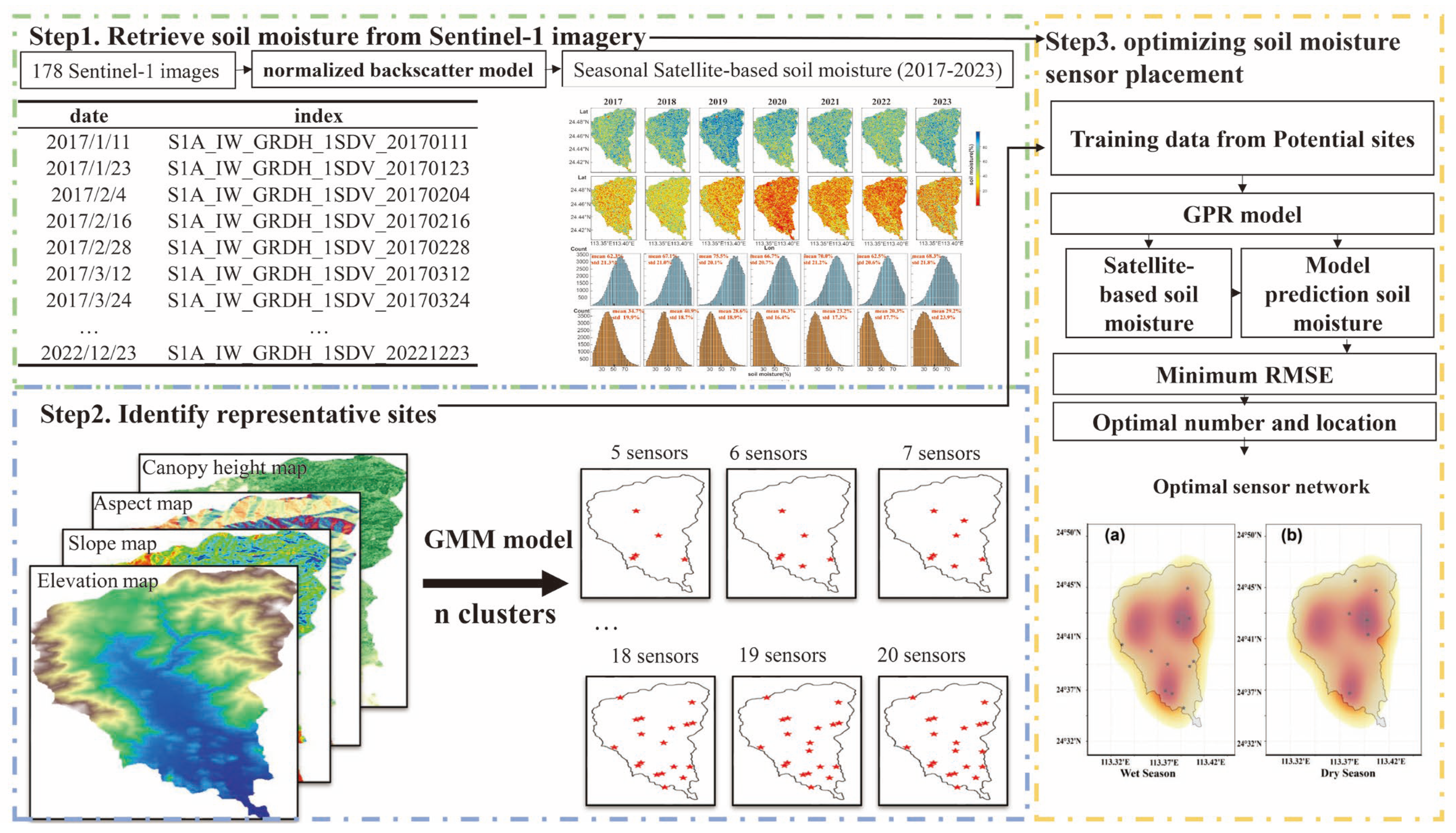
2. Materials and Methods
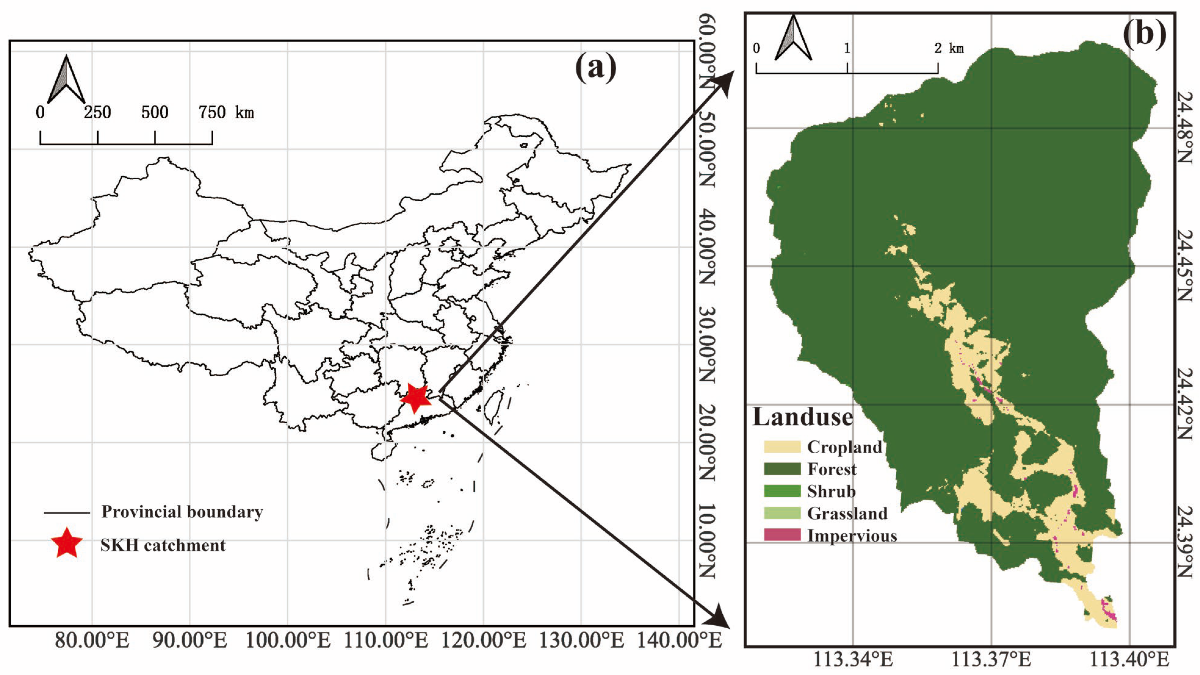
2.1. Study Area
2.2. Input Data and Preprocessing
2.2.1. SAR-Based Soil Moisture Using Sentinel-1 Data
2.2.2. Catchment Physiographic Data
2.3. Machine Learning Models
2.3.1. GMM for Soil Moisture Sensors Clustering
2.3.2. Spatial Prediction Using GPR
2.3.3. Model Evaluation
3. Results
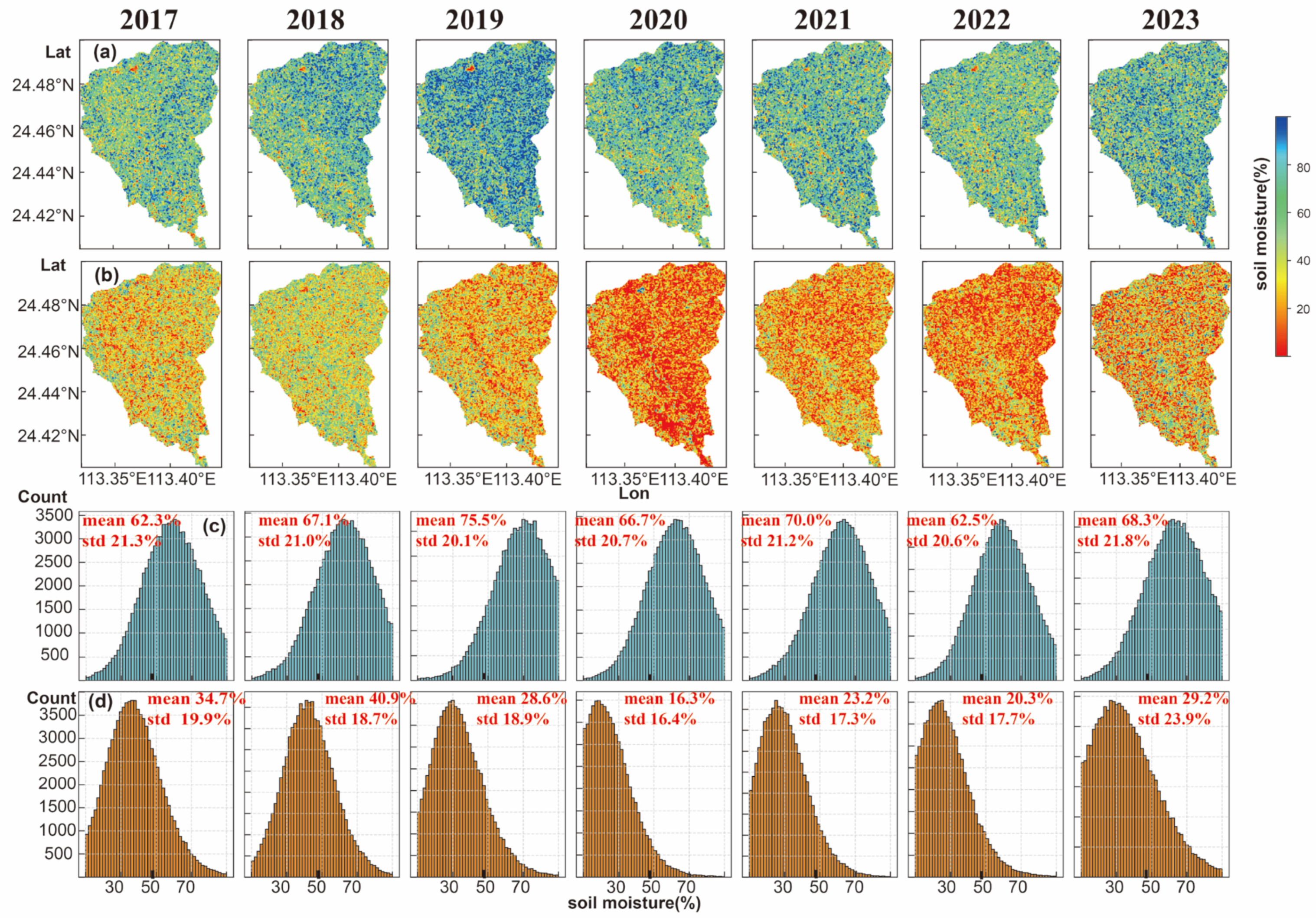
3.1. SAR-Based Soil Moisture in the SKH Catchment
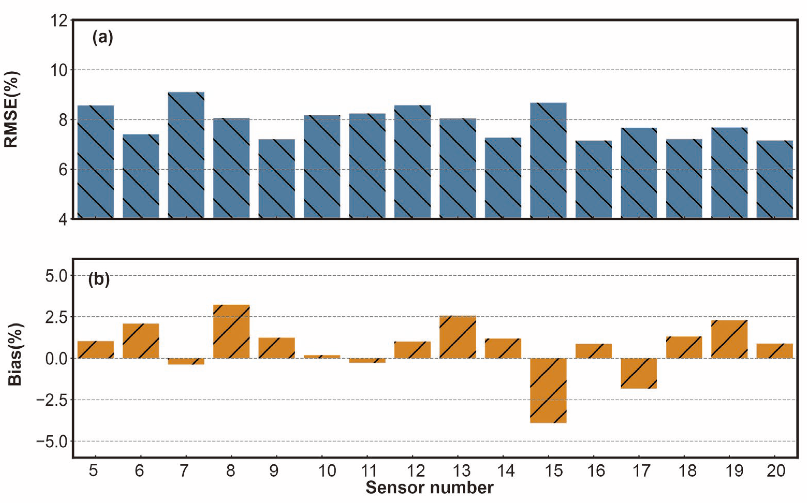
3.2. Model Performance and Optimal Placement of Sensors
3.3. Seasonal Impacts on Optimal Site Selection
3.4. Physiographic Characteristics of Representative Sites
4. Discussion
4.1. Soil Moisture Monitoring Networks for Remote Sensing
4.2. Seasonal Dynamics of Soil Moisture Heterogeneity
4.3. Scaling and Adaptation of Soil Moisture Sensor Network Optimization
4.4. Limitations
5. Conclusions
Supplementary Materials
Author Contributions
Funding
Data Availability Statement
Acknowledgments
Conflicts of Interest
Abbreviations
| WSNs | Wireless Sensor Networks |
| SAR | Synthetic Aperture Radar |
| GPR | Gaussian Process Regression |
| GMM | Gaussian Mixture Model |
| GP | Gaussian Process |
| RMSE | Root Mean Square Error |
| MAE | Mean Absolute Error |
References
- Rodriguez-Iturbe, I. Ecohydrology: A Hydrologic Perspective of Climate-Soil-Vegetation Dynamies. Water Resour. Res. 2000, 36, 3–9. [Google Scholar] [CrossRef]
- Champagne, C.; Berg, A.A.; McNairn, H.; Drewitt, G.; Huffman, T. Evaluation of Soil Moisture Extremes for Agricultural Productivity in the Canadian Prairies. Agric. For. Meteorol. 2012, 165, 1–11. [Google Scholar] [CrossRef]
- Quan, Q.; Liang, W.; Yan, D.; Lei, J. Influences of Joint Action of Natural and Social Factors on Atmospheric Process of Hydrological Cycle in Inner Mongolia, China. Urban. Clim. 2022, 41, 101043. [Google Scholar] [CrossRef]
- Zhang, K.; Ali, A.; Antonarakis, A.; Moghaddam, M.; Saatchi, S.; Tabatabaeenejad, A.; Chen, R.; Jaruwatanadilok, S.; Cuenca, R.; Crow, W.T.; et al. The Sensitivity of North American Terrestrial Carbon Fluxes to Spatial and Temporal Variation in Soil Moisture: An Analysis Using Radar-Derived Estimates of Root-Zone Soil Moisture. J. Geophys. Res. Biogeosciences 2019, 124, 3208–3231. [Google Scholar] [CrossRef]
- Morbidelli, R.; Saltalippi, C.; Flammini, A.; Corradini, C.; Brocca, L.; Govindaraju, R.S. An Investigation of the Effects of Spatial Heterogeneity of Initial Soil Moisture Content on Surface Runoff Simulation at a Small Watershed Scale. J. Hydrol. 2016, 539, 589–598. [Google Scholar] [CrossRef]
- He, M.; Kimball, J.S.; Running, S.; Ballantyne, A.; Guan, K.; Huemmrich, F. Satellite Detection of Soil Moisture Related Water Stress Impacts on Ecosystem Productivity Using the MODIS-Based Photochemical Reflectance Index. Remote Sens. Environ. 2016, 186, 173–183. [Google Scholar] [CrossRef]
- Furtak, K.; Wolińska, A. The Impact of Extreme Weather Events as a Consequence of Climate Change on the Soil Moisture and on the Quality of the Soil Environment and Agriculture—A Review. Catena 2023, 231, 107378. [Google Scholar] [CrossRef]
- Liu, Y.; Yang, Y. Advances in the Quality of Global Soil Moisture Products: A Review. Remote Sens. 2022, 14, 3741. [Google Scholar] [CrossRef]
- Feng, Q.; Zhao, W.; Qiu, Y.; Zhao, M.; Zhong, L. Spatial Heterogeneity of Soil Moisture and the Scale Variability of Its Influencing Factors: A Case Study in the Loess Plateau of China. Water 2013, 5, 1226–1242. [Google Scholar] [CrossRef]
- Stark, J.R.; Fridley, J.D. Topographic Drivers of Soil Moisture Across a Large Sensor Network in the Southern Appalachian Mountains (USA). Water Resour. Res. 2023, 59, e2022WR034315. [Google Scholar] [CrossRef]
- Lakhankar, T.; Ghedira, H.; Temimi, M.; Azar, A.E.; Khanbilvardi, R. Effect of Land Cover Heterogeneity on Soil Moisture Retrieval Using Active Microwave Remote Sensing Data. Remote Sens. 2009, 1, 80–91. [Google Scholar] [CrossRef]
- Stanyer, C.; Seco-Rizo, I.; Atzberger, C.; Marti-Cardona, B. Soil Texture, Soil Moisture, and Sentinel-1 Backscattering: Towards the Retrieval of Field-Scale Soil Hydrological Properties. Remote Sens. 2025, 17, 542. [Google Scholar] [CrossRef]
- Munda, M.K.; Parida, B.R. Soil Moisture Modeling over Agricultural Fields Using C-Band Synthetic Aperture Radar and Modified Dubois Model. Appl. Geomat. 2023, 15, 97–108. [Google Scholar] [CrossRef]
- Zhu, L.; Cai, Q.; Jin, J.; Yuan, S.; Shen, X.; Walker, J.P. Multi-Scale Domain Adaptation for High-Resolution Soil Moisture Retrieval from Synthetic Aperture Radar in Data-Scarce Regions. J. Hydrol. 2025, 657, 133073. [Google Scholar] [CrossRef]
- Wigneron, J.-P.; Calvet, J.-C.; Pellarin, T.; Van De Griend, A.A.; Berger, M.; Ferrazzoli, P. Retrieving Near-Surface Soil Moisture from Microwave Radiometric Observations: Current Status and Future Plans. Remote Sens. Environ. 2003, 85, 489–506. [Google Scholar] [CrossRef]
- Duarte, E.; Hernandez, A. A Review on Soil Moisture Dynamics Monitoring in Semi-Arid Ecosystems: Methods, Techniques, and Tools Applied at Different Scales. Appl. Sci. 2024, 14, 7677. [Google Scholar] [CrossRef]
- Li, X.; Li, X.; Li, Z.; Ma, M.; Wang, J.; Xiao, Q.; Liu, Q.; Che, T.; Chen, E.; Yan, G.; et al. Watershed Allied Telemetry Experimental Research. J. Geophys. Res. Atmos. 2009, 114, D22103. [Google Scholar] [CrossRef]
- Merlin, O.; Walker, J.P.; Kalma, J.D.; Kim, E.J.; Hacker, J.; Panciera, R.; Young, R.; Summerell, G.; Hornbuckle, J.; Hafeez, M.; et al. The NAFE’06 Data Set: Towards Soil Moisture Retrieval at Intermediate Resolution. Adv. Water Resour. 2008, 31, 1444–1455. [Google Scholar] [CrossRef]
- Panciera, R.; Walker, J.P.; Jackson, T.J.; Gray, D.A.; Tanase, M.A.; Ryu, D.; Monerris, A.; Yardley, H.; Rüdiger, C.; Wu, X.; et al. The Soil Moisture Active Passive Experiments (SMAPEx): Toward Soil Moisture Retrieval From the SMAP Mission. IEEE Trans. Geosci. Remote Sens. 2014, 52, 490–507. [Google Scholar] [CrossRef]
- Li, X.; Cheng, G.; Liu, S.; Xiao, Q.; Ma, M.; Jin, R.; Che, T.; Liu, Q.; Wang, W.; Qi, Y.; et al. Heihe Watershed Allied Telemetry Experimental Research (HiWATER): Scientific Objectives and Experimental Design. Bull. Am. Meteorol. Soc. 2013, 94, 1145–1160. [Google Scholar] [CrossRef]
- Rasheed, M.W.; Tang, J.; Sarwar, A.; Shah, S.; Saddique, N.; Khan, M.U.; Imran Khan, M.; Nawaz, S.; Shamshiri, R.R.; Aziz, M.; et al. Soil Moisture Measuring Techniques and Factors Affecting the Moisture Dynamics: A Comprehensive Review. Sustainability 2022, 14, 11538. [Google Scholar] [CrossRef]
- Briciu-Burghina, C.; Zhou, J.; Ali, M.I.; Regan, F. Demonstrating the Potential of a Low-Cost Soil Moisture Sensor Network. Sensors 2022, 22, 987. [Google Scholar] [CrossRef]
- Kerkez, B.; Glaser, S.D.; Bales, R.C.; Meadows, M.W. Design and Performance of a Wireless Sensor Network for Catchment-scale Snow and Soil Moisture Measurements. Water Resour. Res. 2012, 48, W09515. [Google Scholar] [CrossRef]
- Martini, E.; Bauckholt, M.; Kögler, S.; Kreck, M.; Roth, K.; Werban, U.; Wollschläger, U.; Zacharias, S. STH-Net: A Soil Monitoring Network for Process-Based Hydrological Modelling from the Pedon to the Hillslope Scale. Earth Syst. Sci. Data 2021, 13, 2529–2539. [Google Scholar] [CrossRef]
- Bogena, H.R.; Herbst, M.; Huisman, J.A.; Rosenbaum, U.; Weuthen, A.; Vereecken, H. Potential of Wireless Sensor Networks for Measuring Soil Water Content Variability. Vadose Zone J. 2010, 9, 1002–1013. [Google Scholar] [CrossRef]
- Placidi, P.; Gasperini, L.; Grassi, A.; Cecconi, M.; Scorzoni, A. Characterization of Low-Cost Capacitive Soil Moisture Sensors for IoT Networks. Sensors 2020, 20, 3585. [Google Scholar] [CrossRef]
- Abdulwahid, H.M.; Mishra, A. Deployment Optimization Algorithms in Wireless Sensor Networks for Smart Cities: A Systematic Mapping Study. Sensors 2022, 22, 5094. [Google Scholar] [CrossRef]
- Liang, J.; Tian, M.; Liu, Y.; Zhou, J. Coverage Optimization of Soil Moisture Wireless Sensor Networks Based on Adaptive Cauchy Variant Butterfly Optimization Algorithm. Sci. Rep. 2022, 12, 11687. [Google Scholar] [CrossRef]
- Xiao, J.; Liu, Y.; Zhou, J. Quantum Clone Elite Genetic Algorithm-Based Evaluation Mechanism for Maximizing Network Efficiency in Soil Moisture Wireless Sensor Networks. J. Sens. 2021, 2021, 5590472. [Google Scholar] [CrossRef]
- Dursun, M.; Özden, S. Optimization of Soil Moisture Sensor Placement for a PV-Powered Drip Irrigation System Using a Genetic Algorithm and Artificial Neural Network. Electr. Eng. 2017, 99, 407–419. [Google Scholar] [CrossRef]
- Haseeb, K.; Ud Din, I.; Almogren, A.; Islam, N. An Energy Efficient and Secure IoT-Based WSN Framework: An Application to Smart Agriculture. Sensors 2020, 20, 2081. [Google Scholar] [CrossRef] [PubMed]
- Bessenbacher, V.; Gudmundsson, L.; Seneviratne, S.I. Optimizing Soil Moisture Station Networks for Future Climates. Geophys. Res. Lett. 2023, 50, e2022GL101667. [Google Scholar] [CrossRef]
- Oroza, C.A.; Zheng, Z.; Glaser, S.D.; Tuia, D.; Bales, R.C. Optimizing Embedded Sensor Network Design for Catchment-Scale Snow-Depth Estimation Using LiDAR and Machine Learning: Optimizing Snow Sensor Placements. Water Resour. Res. 2016, 52, 8174–8189. [Google Scholar] [CrossRef]
- Yang, J.; Huang, X. The 30 m Annual Land Cover Dataset and Its Dynamics in China from 1990 to 2019. Earth Syst. Sci. Data 2021, 13, 3907–3925. [Google Scholar] [CrossRef]
- Xu, Q.; Yang, Y.; Yang, R.; Zha, L.-S.; Lin, Z.-Q.; Shang, S.-H. Spatial Trade-Offs and Synergies between Ecosystem Services in Guangdong Province, China. Land 2024, 13, 32. [Google Scholar] [CrossRef]
- Jiang, S.; Guo, X.; Zhao, P.; Liang, H. Radial Growth–Climate Relationship Varies with Spatial Distribution of Schima Superba Stands in Southeast China’s Subtropical Forests. Forests 2023, 14, 1291. [Google Scholar] [CrossRef]
- Yu, B.; Kang, J.; Tang, J.; Wang, Z.; Zhang, S.; Ma, Q.; Su, H. Effect of Nitrogen Addition on the Intra-Annual Leaf and Stem Traits and Their Relationships in Two Dominant Species in a Subtropical Forest. Forests 2025, 16, 28. [Google Scholar] [CrossRef]
- Tao, L.; Wang, G.; Chen, W.; Chen, X.; Li, J.; Cai, Q. Soil Moisture Retrieval from SAR and Optical Data Using a Combined Model. IEEE J. Sel. Top. Appl. Earth Obs. Remote Sens. 2019, 12, 637–647. [Google Scholar] [CrossRef]
- Kornelsen, K.C.; Coulibaly, P. Advances in Soil Moisture Retrieval from Synthetic Aperture Radar and Hydrological Applications. J. Hydrol. 2013, 476, 460–489. [Google Scholar] [CrossRef]
- Zeyliger, A.M.; Muzalevskiy, K.V.; Zinchenko, E.V.; Ermolaeva, O.S. Field Test of the Surface Soil Moisture Mapping Using Sentinel-1 Radar Data. Sci. Total Environ. 2022, 807, 151121. [Google Scholar] [CrossRef]
- Monteiro, A.T.; Arenas-Castro, S.; Punalekar, S.M.; Cunha, M.; Mendes, I.; Giamberini, M.; Marques da Costa, E.; Fava, F.; Lucas, R. Remote Sensing of Vegetation and Soil Moisture Content in Atlantic Humid Mountains with Sentinel-1 and 2 Satellite Sensor Data. Ecol. Indic. 2024, 163, 112123. [Google Scholar] [CrossRef]
- Fan, D.; Zhao, T.; Jiang, X.; García-García, A.; Schmidt, T.; Samaniego, L.; Attinger, S.; Wu, H.; Jiang, Y.; Shi, J.; et al. A Sentinel-1 SAR-Based Global 1-Km Resolution Soil Moisture Data Product: Algorithm and Preliminary Assessment. Remote Sens. Environ. 2025, 318, 114579. [Google Scholar] [CrossRef]
- Bauer-Marschallinger, B.; Freeman, V.; Cao, S.; Paulik, C.; Schaufler, S.; Stachl, T.; Modanesi, S.; Massari, C.; Ciabatta, L.; Brocca, L.; et al. Toward Global Soil Moisture Monitoring with Sentinel-1: Harnessing Assets and Overcoming Obstacles. IEEE Trans. Geosci. Remote Sens. 2019, 57, 520–539. [Google Scholar] [CrossRef]
- Wagner, W.; Lemoine, G.; Rott, H. A Method for Estimating Soil Moisture from ERS Scatterometer and Soil Data. Remote Sens. Environ. 1999, 70, 191–207. [Google Scholar] [CrossRef]
- Peng, J.; Loew, A.; Merlin, O.; Verhoest, N.E.C. A Review of Spatial Downscaling of Satellite Remotely Sensed Soil Moisture. Rev. Geophys. 2017, 55, 341–366. [Google Scholar] [CrossRef]
- Dostálová, A.; Doubková, M.; Sabel, D.; Bauer-Marschallinger, B.; Wagner, W. Seven Years of Advanced Synthetic Aperture Radar (ASAR) Global Monitoring (GM) of Surface Soil Moisture over Africa. Remote Sens. 2014, 6, 7683–7707. [Google Scholar] [CrossRef]
- Scipal, K.; Drusch, M.; Wagner, W. Assimilation of a ERS Scatterometer Derived Soil Moisture Index in the ECMWF Numerical Weather Prediction System. Adv. Water Resour. 2008, 31, 1101–1112. [Google Scholar] [CrossRef]
- Wagner, W.; Noll, J.; Borgeaud, M.; Rott, H. Monitoring Soil Moisture over the Canadian Prairies with the ERS Scatterometer. IEEE Trans. Geosci. Remote Sens. 1999, 37, 206–216. [Google Scholar] [CrossRef]
- Liu, A.; Cheng, X.; Chen, Z. Performance Evaluation of GEDI and ICESat-2 Laser Altimeter Data for Terrain and Canopy Height Retrievals. Remote Sens. Environ. 2021, 264, 112571. [Google Scholar] [CrossRef]
- Fayad, I.; Baghdadi, N.; Lahssini, K. An Assessment of the GEDI Lasers’ Capabilities in Detecting Canopy Tops and Their Penetration in a Densely Vegetated, Tropical Area. Remote Sens. 2022, 14, 2969. [Google Scholar] [CrossRef]
- Schneider, K.; Helfricht, K.; Sailer, R.; Kuhn, M.; Schöber, J. Interannual Persistence of the Seasonal Snow Cover in a Glacierized Catchment. J. Glaciol. 2014, 60, 889–904. [Google Scholar]
- Bukkapatnam, S.T.S.; Cheng, C. Forecasting the Evolution of Nonlinear and Nonstationary Systems Using Recurrence-Based Local Gaussian Process Models. Phys. Rev. E Stat. Nonlin. Soft Matter Phys. 2010, 82, 056206. [Google Scholar] [CrossRef] [PubMed]
- Rasmussen, C.E.; Williams, C.K.I. Gaussian Processes for Machine Learning; The MIT Press: Cambridge, MA, USA, 2005; ISBN 978-0-262-25683-4. [Google Scholar]
- Zhang, X.; Sun, X.; Lin, Z. Improving Soil Moisture Prediction Using Gaussian Process Regression. Smart Agric. Technol. 2025, 11, 100905. [Google Scholar] [CrossRef]
- Jackson, T.J.; Bindlish, R.; Cosh, M.H.; Zhao, T.; Starks, P.J.; Bosch, D.D.; Seyfried, M.; Moran, M.S.; Goodrich, D.C.; Kerr, Y.H.; et al. Validation of Soil Moisture and Ocean Salinity (SMOS) Soil Moisture Over Watershed Networks in the U.S. IEEE Trans. Geosci. Remote Sens. 2012, 50, 1530–1543. [Google Scholar] [CrossRef]
- Li, X.; Ling, F.; Foody, G.M.; Ge, Y.; Zhang, Y.; Du, Y. Generating a Series of Fine Spatial and Temporal Resolution Land Cover Maps by Fusing Coarse Spatial Resolution Remotely Sensed Images and Fine Spatial Resolution Land Cover Maps. Remote Sens. Environ. 2017, 196, 293–311. [Google Scholar] [CrossRef]
- Narayanan, R.M.; Ponnappan, S.K.; Reichenbach, S.E. Effects of Noise on the Information Content of Remote Sensing Images. Geocarto Int. 2003, 18, 15–26. [Google Scholar] [CrossRef]
- Sayer, A.M.; Govaerts, Y.; Kolmonen, P.; Lipponen, A.; Luffarelli, M.; Mielonen, T.; Patadia, F.; Popp, T.; Povey, A.C.; Stebel, K. A Review and Framework for the Evaluation of Pixel-Level Uncertainty Estimates in Satellite Aerosol Remote Sensing. Atmos. Meas. Tech. 2020, 13, 373–404. [Google Scholar] [CrossRef]
- Chang, N.-B.; Makkeasorn, A. Optimal Site Selection of Watershed Hydrological Monitoring Stations Using Remote Sensing and Grey Integer Programming. Environ. Model. Assess. 2010, 15, 469–486. [Google Scholar] [CrossRef]
- Su, L.; Wang, J.; Qin, X.; Wang, Q. Approximate Solution of a One-Dimensional Soil Water Infiltration Equation Based on the Brooks-Corey Model. Geoderma 2017, 297, 28–37. [Google Scholar] [CrossRef]
- Hayek, M. An Exact Explicit Solution for One-Dimensional, Transient, Nonlinear Richards’ Equation for Modeling Infiltration with Special Hydraulic Functions. J. Hydrol. 2016, 535, 662–670. [Google Scholar] [CrossRef]
- Ma, D.; Zhang, J.; Lu, Y.; Wu, L.; Wang, Q. Derivation of the Relationships between Green–Ampt Model Parameters and Soil Hydraulic Properties. Soil Sci. Soc. Am. J. 2015, 79, 1030–1042. [Google Scholar] [CrossRef]
- Rosenbaum, U.; Bogena, H.R.; Herbst, M.; Huisman, J.A.; Peterson, T.J.; Weuthen, A.; Western, A.W.; Vereecken, H. Seasonal and Event Dynamics of Spatial Soil Moisture Patterns at the Small Catchment Scale. Water Resour. Res. 2012, 48, W10544. [Google Scholar] [CrossRef]
- Ivanov, V.Y.; Fatichi, S.; Jenerette, G.D.; Espeleta, J.F.; Troch, P.A.; Huxman, T.E. Hysteresis of Soil Moisture Spatial Heterogeneity and the “Homogenizing” Effect of Vegetation. Water Resour. Res. 2010, 46, W09521. [Google Scholar] [CrossRef]
- Western, A.W.; Blöschl, G.; Grayson, R.B. Geostatistical Characterisation of Soil Moisture Patterns in the Tarrawarra Catchment. J. Hydrol. 1998, 205, 20–37. [Google Scholar] [CrossRef]
- Grayson, R.B.; Western, A.W.; Chiew, F.H.S.; Blöschl, G. Preferred States in Spatial Soil Moisture Patterns: Local and Nonlocal Controls. Water Resour. Res. 1997, 33, 2897–2908. [Google Scholar] [CrossRef]
- Vivoni, E.R.; Rodríguez, J.C.; Watts, C.J. On the Spatiotemporal Variability of Soil Moisture and Evapotranspiration in a Mountainous Basin within the North American Monsoon Region. Water Resour. Res. 2010, 46, W02509. [Google Scholar] [CrossRef]
- Schume, H.; Jost, G.; Katzensteiner, K. Spatio-Temporal Analysis of the Soil Water Content in a Mixed Norway Spruce (Picea abies (L.) Karst.)–European Beech (Fagus sylvatica L.) Stand. Geoderma 2003, 112, 273–287. [Google Scholar] [CrossRef]
- Scanlon, B.R.; Healy, R.W.; Cook, P.G. Choosing Appropriate Techniques for Quantifying Groundwater Recharge. Hydrogeol. J. 2002, 10, 18–39. [Google Scholar] [CrossRef]
- Zhuo, L.; Dai, Q.; Zhao, B.; Han, D. Soil Moisture Sensor Network Design for Hydrological Applications. Hydrol. Earth Syst. Sci. 2020, 24, 2577–2591. [Google Scholar] [CrossRef]
- Ochsner, T.E.; Cosh, M.H.; Cuenca, R.H.; Dorigo, W.A.; Draper, C.S.; Hagimoto, Y.; Kerr, Y.H.; Larson, K.M.; Njoku, E.G.; Small, E.E.; et al. State of the Art in Large-Scale Soil Moisture Monitoring. Soil Sci. Soc. Am. J. 2013, 77, 1888–1919. [Google Scholar] [CrossRef]
- Balenzano, A.; Mattia, F.; Satalino, G.; Lovergine, F.P.; Palmisano, D.; Peng, J.; Marzahn, P.; Wegmüller, U.; Cartus, O.; Dąbrowska-Zielińska, K.; et al. Sentinel-1 Soil Moisture at 1 Km Resolution: A Validation Study. Remote Sens. Environ. 2021, 263, 112554. [Google Scholar] [CrossRef]


| Sensor Number | RMSE (%) | Bias (%) |
|---|---|---|
| 5 | 8.55 | 1.03 |
| 6 | 7.39 | 2.08 |
| 7 | 9.09 | −0.38 |
| 8 | 8.05 | 3.21 |
| 9 | 7.20 | 1.23 |
| 10 | 8.16 | 0.18 |
| 11 | 8.23 | −0.28 |
| 12 | 8.56 | 1.01 |
| 13 | 8.04 | 2.57 |
| 14 | 7.27 | 1.18 |
| 15 | 8.66 | −3.91 |
| 16 | 7.24 | 0.86 |
| 17 | 7.67 | −1.82 |
| 18 | 7.21 | 1.30 |
| 19 | 7.68 | 2.29 |
| 20 | 7.15 | 0.89 |
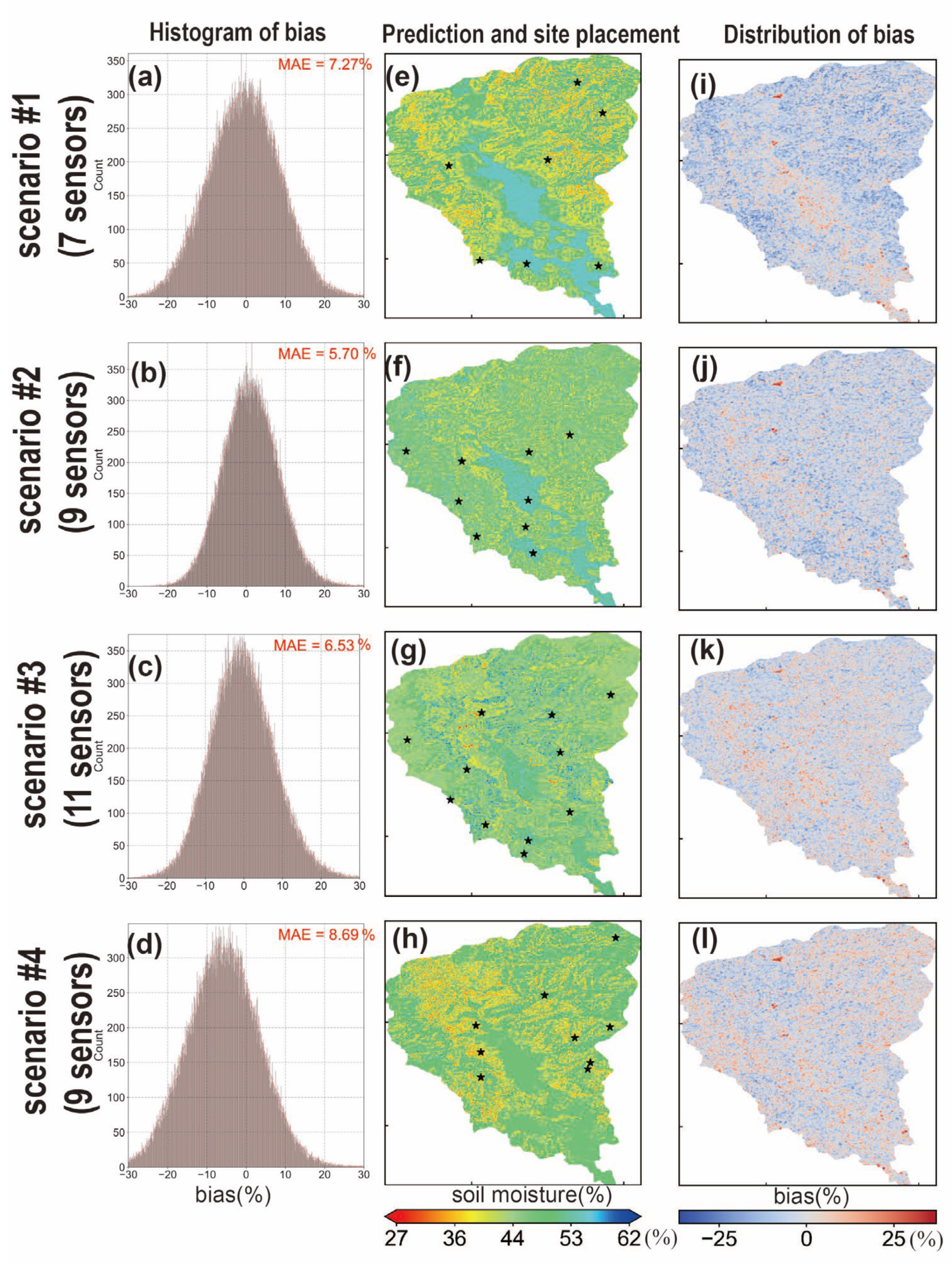
| Scenario | Sensor Number | Site Selection Method | MAE (%) |
|---|---|---|---|
| #1 | 7 | proposed method | 7.27 |
| #2 | 9 | proposed method | 5.70 |
| #3 | 11 | proposed method | 6.53 |
| #4 | 9 | random selection | 8.69 |
Disclaimer/Publisher’s Note: The statements, opinions and data contained in all publications are solely those of the individual author(s) and contributor(s) and not of MDPI and/or the editor(s). MDPI and/or the editor(s) disclaim responsibility for any injury to people or property resulting from any ideas, methods, instructions or products referred to in the content. |
© 2025 by the authors. Licensee MDPI, Basel, Switzerland. This article is an open access article distributed under the terms and conditions of the Creative Commons Attribution (CC BY) license (https://creativecommons.org/licenses/by/4.0/).
Share and Cite
Xie, Y.; Cui, G.; Zheng, K.; Tang, G. Integrating Sentinel-1 SAR and Machine Learning Models for Optimal Soil Moisture Sensor Placement at Catchment Scale. Remote Sens. 2025, 17, 2330. https://doi.org/10.3390/rs17132330
Xie Y, Cui G, Zheng K, Tang G. Integrating Sentinel-1 SAR and Machine Learning Models for Optimal Soil Moisture Sensor Placement at Catchment Scale. Remote Sensing. 2025; 17(13):2330. https://doi.org/10.3390/rs17132330
Chicago/Turabian StyleXie, Yi, Guotao Cui, Kaifeng Zheng, and Guoping Tang. 2025. "Integrating Sentinel-1 SAR and Machine Learning Models for Optimal Soil Moisture Sensor Placement at Catchment Scale" Remote Sensing 17, no. 13: 2330. https://doi.org/10.3390/rs17132330
APA StyleXie, Y., Cui, G., Zheng, K., & Tang, G. (2025). Integrating Sentinel-1 SAR and Machine Learning Models for Optimal Soil Moisture Sensor Placement at Catchment Scale. Remote Sensing, 17(13), 2330. https://doi.org/10.3390/rs17132330