Effects of the October 2024 Storm over the Global Ionosphere

Abstract

The present study analyzes the global ionospheric response to the intense geomagnetic storm of 10–11 October 2024 (SYM—H minimum of −346 nT), using observations from COSMIC—2 and Swarm satellites, GNSS TEC, and Digisondes. Significant uplift of the F-region was observed across both Hemispheres on the dayside, primarily driven by equatorward thermospheric winds and prompt penetration electric fields (PPEFs). However, this uplift did not correspond with increases in foF2 due to enhanced molecular nitrogen-promoting recombination in sunlit regions and the F2 peak rising beyond the COSMIC—2 detection range. In contrast, in the Southern Hemisphere nightside ionosphere exhibited pronounced Ne depletion and low hmF2 values, attributed to G-conditions and thermospheric composition changes caused by storm-time circulation. Strong vertical plasma drifts exceeding 100 m/s were observed during both the main and recovery phases, particularly over Ascension Island, driven initially by southward IMF—Bz-induced PPEFs and later by disturbance dynamo electric fields (DDEFs) as IMF—Bz turned northward. Swarm data revealed a poleward expansion of the Equatorial Ionization Anomaly (EIA), with more pronounced effects in the Southern Hemisphere due to seasonal and longitudinal variations in ionospheric conductivity. Additionally, the storm excited Large-Scale Travelling Ionospheric Disturbances (LSTIDs), triggered by thermospheric perturbations and electrodynamic drivers, including PPEFs and DDEFs. These disturbances, along with enhanced westward thermospheric wind and altered zonal electric fields, modulated ionospheric irregularity intensity and distribution. The emergence of anti-Sq current systems further disrupted quiet-time electrodynamics, promoting global LSTID activity. Furthermore, storm-induced equatorial plasma bubbles (EPBs) were observed over Southeast Asia, initiated by enhanced PPEFs during the main phase and suppressed during recovery, consistent with super EPB development mechanisms.

1. Introduction

Geomagnetic storms have a profound influence on Earth’s ionosphere across all latitudes, triggering intricate physical processes in equatorial, midlatitude, and polar regions. These interactions complicate our understanding of space weather dynamics [1,2,3,4,5,6,7]. Storm-time electric field and energy input from the magnetosphere can induce rapid ionospheric responses, sometimes intensifying ionospheric instabilities [8,9], while at other times suppressing them [10,11], depending on local conditions and time scales.

During Solar Cycle 25, two significant geomagnetic storms—classified as G4 and G5—occurred in 2024, coinciding with a peak in solar activity. The most intense of these was the G5-class “Mother’s Day Storm” on 10–11 May 2024 (Kp~9), one of the strongest storms since 1957. This event generated auroras visible at midlatitudes (~45°N and ~37°S) [12,13]. Spogli et al. (2024) [14] reported major space weather effects over Italy, notably a substantial drop in plasma density on 11 May, resulting in a negative ionospheric storm evident in both F-layer critical frequency (foF2) and total electron content (TEC). This was linked to changes in the thermospheric composition, particularly a decrease in the [O/N2] ratio. High values of the Rate of TEC Change Index (ROTI) were also observed, associated with Stable Auroral Red (SAR) arcs and a southward shift in the ionospheric trough. The ROTI enhancement was attributed to low-latitude plasma being driven poleward by pre-reversal enhancement (PRE) after sunset, along with northward-propagating wave-like disturbances. Karan et al. (2024) [13], using NASA’s GOLD imager, identified a connection between the southern crest of the Equatorial Ionization Anomaly (EIA) and auroral activity near the southern tip of South America. The EIA crest shifted poleward at speeds up to 450 m/s, and auroral emission extended to midlatitudes over Southern Africa and South America, resulting in midlatitude plasma erosion. Themens et al. (2024) [15] described a significant uplift in the Storm-Enhanced Density (SED) plume, with the F2-layer height (hmF2) rising by 150–300 km and GNSS scintillation observed across the auroral oval. Bojilova et al. (2024) [16] reported Hemispheric asymmetries in the ionospheric response due to particle precipitation and thermospheric heating, along with EIA modifications and disturbance dynamo electric fields (DDEFs) at lower latitudes. Paul et al. (2025) [5] investigated the ionospheric response over Europe during the Mother’s Day storm using Digisonde data and Swarm satellite measurements. They found notable Ne depletion, attributed to the equatorward shift in the Midlatitude Ionospheric Trough (MIT). Large-Scale Travelling Ionospheric Disturbances (LSTIDs) and Spread F were also evident, primarily at higher midlatitudes. A broader study by Paul et al. (2025) [6] showed global-scale F2-layer uplift and increased foF2 over midlatitude dayside regions, while nightside values decreased. Enhanced vertical and horizontal plasma drifts were observed, including ~170 m/s upward drift in the Southern Hemisphere during the storm’s main phase. Swarm A measurements indicated EIA expansion to 60°S on the dayside and 40°S on the nightside.

The second major G4-class storm occurred on 10–11 October 2024. This event has received limited attention so far. Pierrard et al. (2025) [17] were among the first to offer an analysis, comparing the October storm to the May G5 event. Using Vertical TEC (VTEC) and ionosonde data from Europe, the USA, and South Korea, they found that upper atmospheric ionization initially spiked after Coronal Mass Ejection (CME) arrival, followed by a prolonged depletion lasting over 24 h. Recovery began on October 12, whereas the May event showed an unusually fast rebound. These effects were attributed to intense F-layer perturbation, further amplified by plasmaspheric contribution to VTEC variation. Picanço et al. (2025) [18] described a reversed C-shaped depletion band stretching from the magnetic equator to auroral latitudes. This feature was driven by intensified vertical drift at the equator and zonal drift at higher latitudes, causing the polar irregularity region to extend into midlatitudes and merge with elongated equatorial plasma bubble (EPB) structures around ~45° MLAT. They observed longitudinal asymmetry in EPB development: along South America’s western coast (~0° MLON), EPB activity appeared at midlatitudes, while along the eastern coast (~20° MLON), it remained equator-bound. These patterns were linked to differences in electric field penetration efficiency due to seasonal changes in ionospheric conductivity. Additionally, DDEFs sustained elevated F-region altitudes and triggered rare post-sunrise EPBs.

By incorporating a wide range of satellite and ground-based observations, the present analysis investigates the global ionospheric response to the 10–11 October 2024 geomagnetic storm. Using Constellation Observing System for Meteorology, Ionosphere, and Climate—2 (COSMIC—2) RO profiles, in situ Ne measurements from Swarm satellites, ion drift data from Digisondes, and global TEC maps, the analysis offers a comprehensive view of storm-time ionospheric dynamics, particularly over equatorial and midlatitude regions and at higher altitudes where significant plasma redistribution occurs. Additional validation from far-ultraviolet emissions from the GUVI instrument aboard TIMED supported the findings. The present article is organized into six sections. Section 1 provides an overview of existing literature on both May and October 2024 geomagnetic storms, offering essential context and comparative insight into the characteristics, impact, and underlying dynamics of these two significant space weather events. Section 2 describes the data sources and the methodology. Section 3 examines the solar and geomagnetic activity associated with the event. Section 4 presents the results, followed by Section 5, which discusses the findings in the context of physical processes driving ionospheric variability. Finally, Section 6 summarizes the key observations and insights.

2. Data and Methods

As a first step in our investigation of the 10–11 October 2024 geomagnetic storm, we examined solar activity using solar and solar wind data from the SOHO/LASC–C2 instrument. These observations, covering the period from 10 to 12 October 2024, were accessed via the SOHO data repository (https://soho.nascom.nasa.gov/data/data.html accessed on 23 April 2025) to identify key solar features such as CMEs and their potential geoeffectiveness. To characterize geomagnetic conditions during the storm, we utilized high-resolution (1 min) OMNI data provided by NASA’s Goddard Space Flight Center (http://omniweb.gsfc.nasa.gov accessed on 23 April 2025) and supplemented it with geomagnetic indices from the International Service of Geomagnetic Indices (https://isgi.unistra.fr/indices_asy.php accessed on 23 April 2025).

To analyze the ionospheric response globally, we focused on F2-layer peak characteristics—foF2 and hmF2—across low to midlatitudes from the COSMIC—2 RO mission, provided by the University Corporation for Atmospheric Research (UCAR). Specifically, we used Level 2 “ionPrf” data files from the COSMIC Data Analysis and Archive Center (CDAAC), which contain electron density (Ne) profiles with respect to altitude derived via Abel inversion from slant TEC observations. Due to the low inclination of COSMIC—2 satellites, coverage is optimized for latitudes within ±35° magnetic (~±45° geographic), making it ideal for equatorial and low- to midlatitude ionospheric studies [6].

To examine ionospheric drift velocities during the storm, we extracted vertical (Vz) and horizontal (Vnorth and Veast) drift velocities from the University of Massachusetts Lowell Center for Atmospheric Research (UMLCAR) Digisonde drift database (https://lgdc.uml.edu/common/DFDBFastStationList accessed on 23 April 2025). Due to limited data availability, we focused on three stations: Lualualei (21.43°N–158.15°E), Eglin (30.5°N–86.5°E), and Ascension Island (−7.95°N–14.4°E). Drift velocities from 00:00 UT on 10 October to 02:00 UT on 12 October were extracted using the DriftExplorer (version 1.2.14) tool (https://ulcar.uml.edu/Drift-X.html accessed on 23 April 2025), offering insight into the electric field-driven plasma transport across different latitudes.

Thermospheric composition data, particularly the atomic oxygen to molecular nitrogen ratio [O/N₂], were obtained from the Global Ultraviolet Imager (GUVI) instrument onboard the TIMED spacecraft. These data, covering the period from 10 to 12 October, were accessed from the GUVI data portal (http://guvitimed.jhuapl.edu/data_products accessed on 25 April 2025) with October 6 as a reference. This compositional ratio serves as a critical indicator of neutral atmospheric dynamics that influence electron density during geomagnetic storms.

In addition to these datasets, we analyzed in situ Ne measurements from the Swarm A and B satellite Langmuir probes (LP), accessed through the ESA’s VirES platform (https://vires.services/ accessed on 24 April 2024). The Swarm mission consists of three identical satellites (Swarm A, B, and C) in near-polar orbits, with Swarm A and C initially orbiting at ~465 km and Swarm B at ~520 km [19]. These high-altitude, high-resolution observations are essential for capturing storm-induced changes in Ne at F-region altitudes.

To support a comprehensive global-scale analysis of ionospheric variability, we employed TEC data derived from the Madrigal database (http://www.haystack.mit.edu accessed on 24 April 2025)—a widely recognized open-source platform developed by the MIT Haystack Observatory. Madrigal (Millstone Analysis and Data Reduction Interactive Graphical Analysis Language) is a distributed data system that hosts and serves a wide range of geospace science data, including ionospheric and upper atmospheric measurements. It enables users to perform advanced data searches and supports access to standardized data formats that are compatible with systems such as the NCAR CEDAR data archive [6]. Specifically, we utilized global GPS-derived TEC maps available through Madrigal’s “Distributed Ground-Based Satellite Receivers” instrument category, and more precisely from the “Worldwide GNSS Receiver Network” dataset. This dataset provides near-real-time, globally distributed TEC maps generated from ground-based GNSS observations. The TEC values are mapped into a regular spatial grid of 1° latitude × 1° longitude, with a temporal resolution of 5 min, offering high-resolution coverage suitable for monitoring large-scale ionospheric structures and their temporal evolution. For this study, we extracted global TEC maps spanning the interval from 18:00 UT on 10 October to 18:00 UT on 11 October. These maps represent processed and calibrated TEC data, which are derived through the integration of dual-frequency GNSS signal phase delays measured at a global network of ground-based receivers. The integration time for each global TEC map is approximately 20 min, providing a temporally smoothed view of ionospheric electron density distribution across the globe. The selected dataset spans more than two decades (1998 to present), making it one of the most comprehensive and accessible sources for long-term ionospheric research.

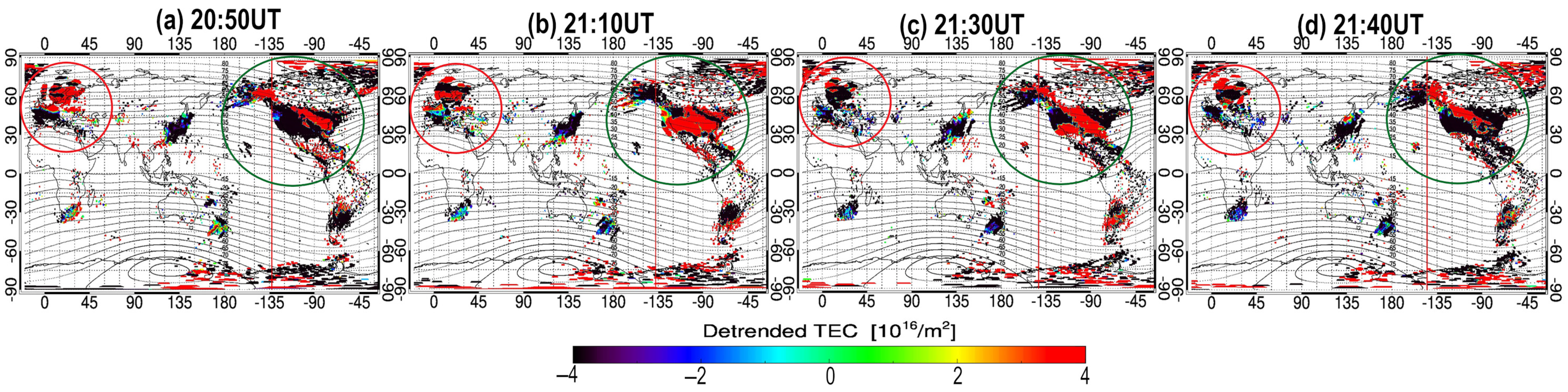
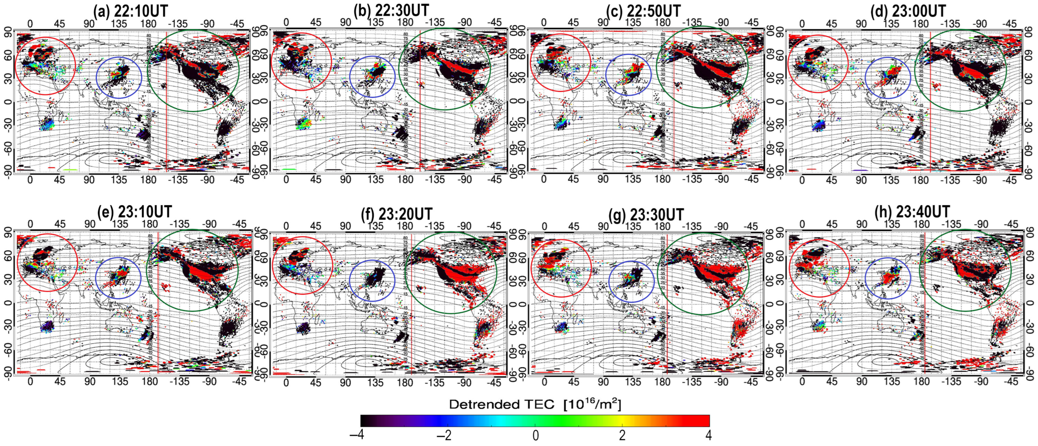
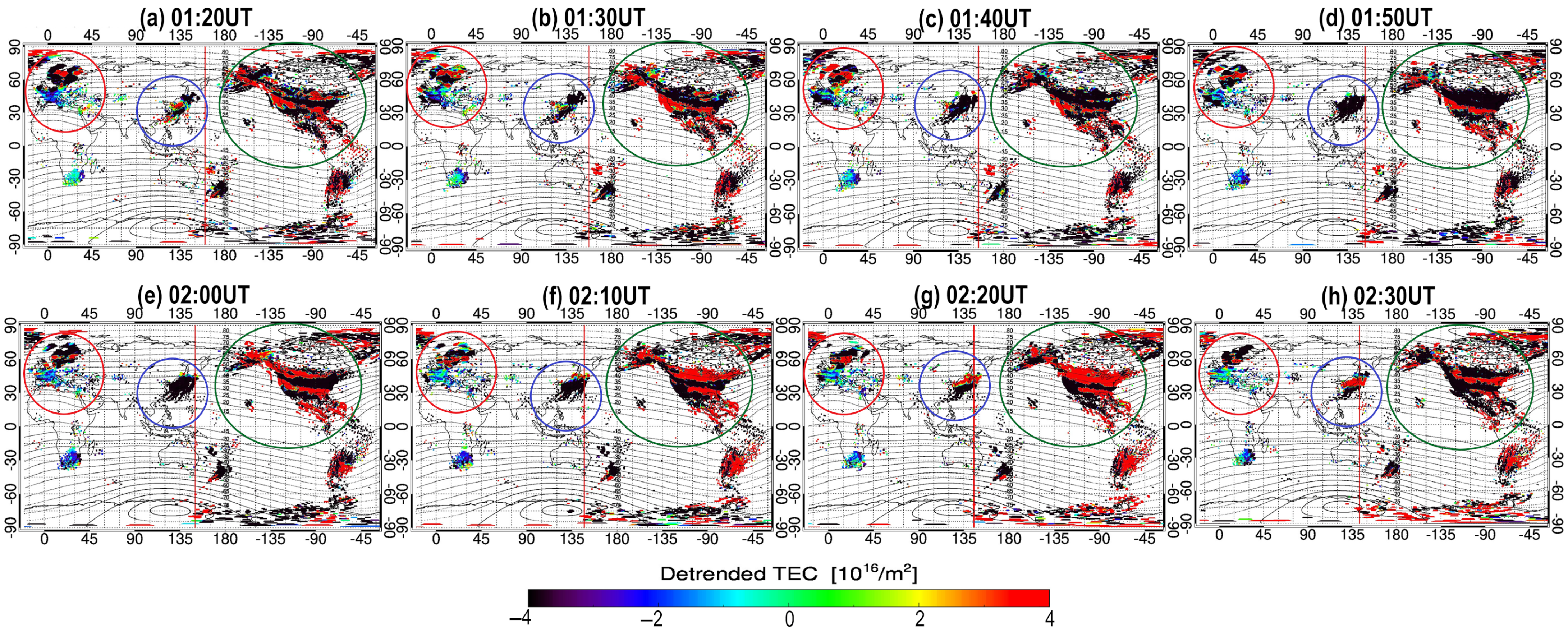
To investigate the activity of LSTIDs during the main phase of the geomagnetic storm, we employed global detrended TEC (dTEC) maps spanning from 15:00 UT on 10 October to 03:00 UT on 11 October. These maps were obtained from the GPS-TEC database maintained by Nagoya University (https://stdb2.isee.nagoya-u.ac.jp/GPS/GPS-TEC/GLOBAL/MAP/index.html#Oct%202024 accessed on 26 April 2025), which offers multiple two-dimensional ionospheric data products, including the absolute TEC, the TEC difference ratio (rTEC), the detrended TEC (dTEC), and the ROTI. All data products are provided in geographic coordinates with a temporal resolution of 10 min. The dTEC maps used in this study are generated using data from over 9300 GNSS receivers distributed globally. The global RINEX files used for generating these maps were collected through international collaboration with the DRAWING-TEC project managed by the National Institute of Information and Communications Technology (NICT), Japan (https://aer-nc-web.nict.go.jp/GPS/DRAWING-TEC/ accessed on 26 April 2025). To derive dTEC values, the bias estimation technique proposed by Otsuka et al. (2002) [20] was applied, ensuring accurate baseline corrections. The dTEC product specifically isolates ionospheric anomalies by removing long-term trends from the TEC data. For improved spatial resolution and reduced noise, the data are gridded at 0.25° × 0.25° in geographic latitude and longitude and smoothed using a 5 × 5 grid boxcar averaging method. This enhances the spatial continuity of the ionospheric features while preserving significant perturbation signatures associated with LSTIDs.

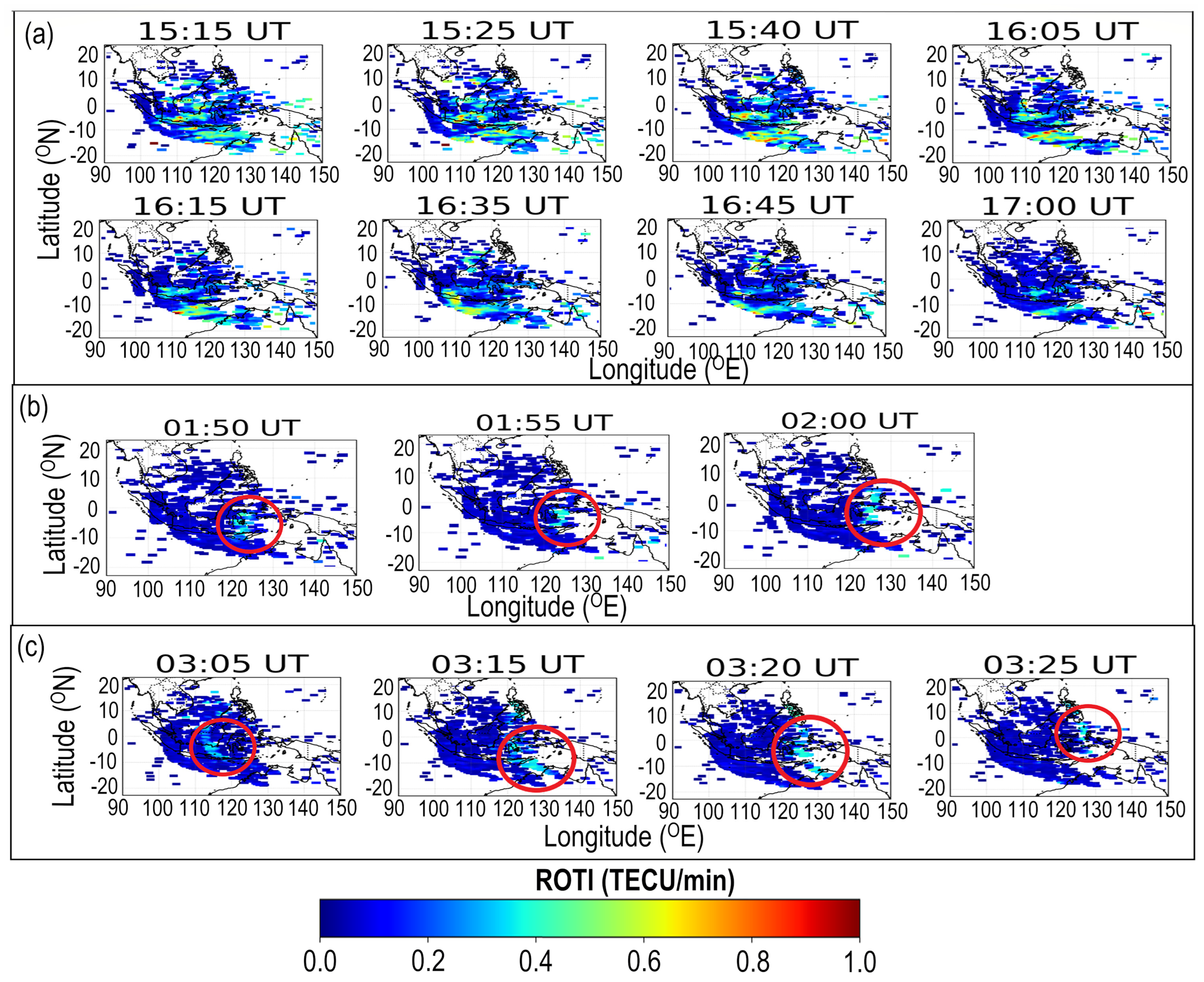
Although the previously discussed global dTEC maps provide comprehensive coverage of ionospheric perturbations, their spatial resolution and data density are notably limited over the Southern Hemisphere, particularly in the Asian-Australian longitude sector. To address this gap and enable a more detailed investigation of ionospheric irregularities in this region, we utilized ROTI data from the Ina-CORS GNSS network, available through the BRIN Ionospheric Map Service (https://gatotkaca.brin.go.id/petaionosfer/ionosphericmap/roti_map/ accessed on 20 June 2025) for the period spanning 15:00 UT on 10 October to 20:00 UT on 11 October. The Ina-CORS network comprises approximately 300 GNSS receivers distributed across the Indonesian archipelago, covering a longitudinal range from 95°E to 140°E and a latitudinal extent from 5°N to 10°S. These stations record GNSS observations at a 30 s cadence, with data stored in the RINEX format. TEC values derived from these observations are used to compute the ROTI, which is defined as the standard deviation of the TEC rate of change over a 5 min sliding window. This metric is a well-established proxy for identifying ionospheric irregularities, particularly those associated with EPBs, which occur at spatial scales of a few kilometres. For visualization, ROTI values are mapped at an Ionospheric Pierce Point (IPP) altitude of 350 km, generating two-dimensional latitude–longitude grids at a resolution of 0.25° × 0.25°. To enhance spatial coherence and reduce noise, a 5 × 5 boxcar averaging filter is applied across the grid. ROTI maps are generated at 10 min intervals between 09:00 and 23:50 UT, offering high temporal resolution snapshots of ionospheric activity over Indonesia. The ROTI map grid consists of a 241 × 161 matrix, encompassing a geographic area bounded by longitudes 90°E to 150°E and latitudes −20°N to 20°N. Missing data points are denoted by “NaN” values.

3. Solar and Geomagnetic Activity

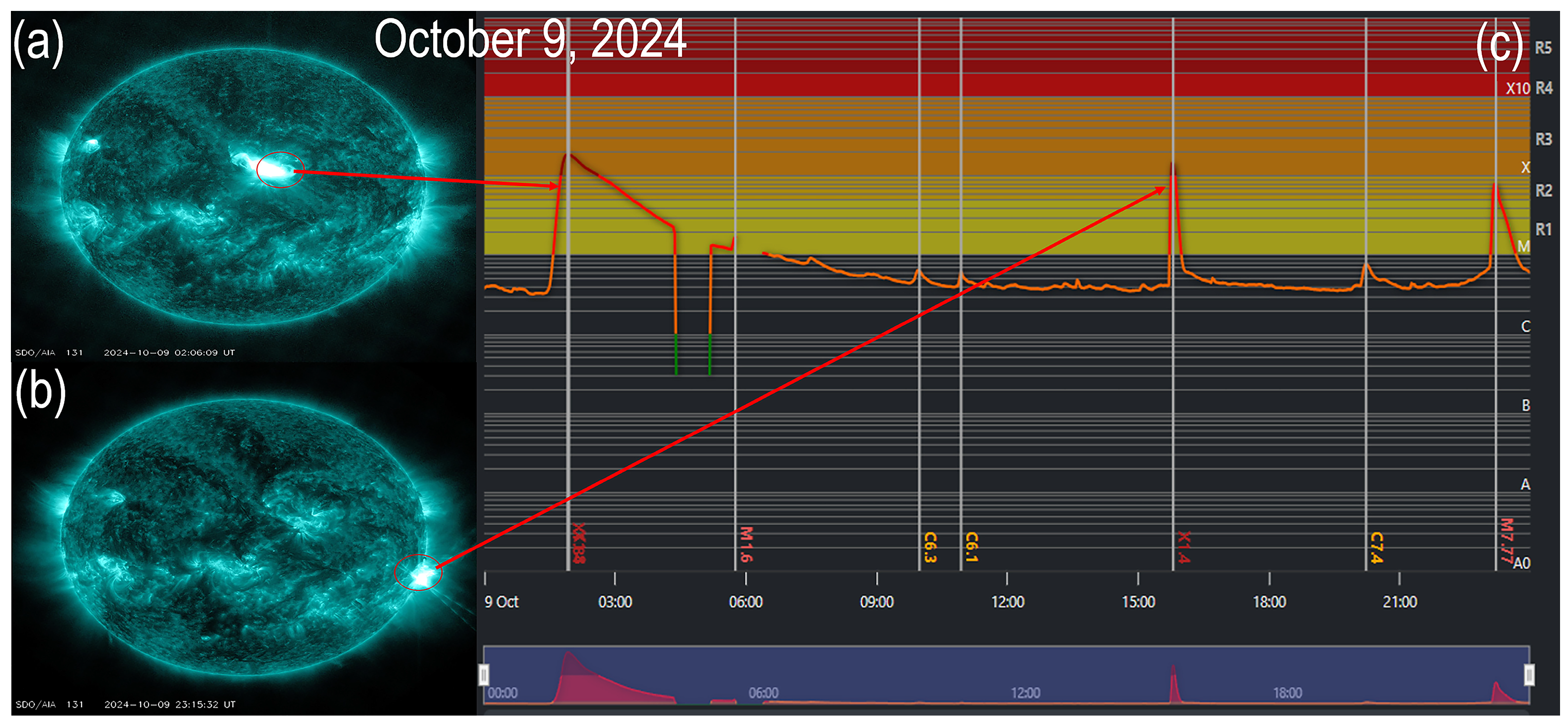
The October 2024 geomagnetic storm was triggered by two highly active solar regions identified by NOAA as AR3848 and AR3842. These regions generated a series of powerful solar flares, including two classified as X-class—the most intense category, known for their strong X-ray emissions and frequent association with fast and wide CMEs. On 9 October, AR3848 and AR3842 collectively produced two M-class, three C-class, and two X-class flares (Figure 1a–c). The first of these, an X1.8 flare from AR3848, began at 01:25 UT, peaked around 01:56 UT, and ended by 02:43 UT. Later that day, an X1.4 flare from AR3842 erupted, starting at 15:44 UT, peaking at 15:47 UT, and fading by 15:53 UT (https://www.spaceweatherlive.com/en/archive/2024/10/09/xray.html accessed on 23 April 2025). The first CME associated with the X1.8 flare was observed by SOHO/LASCO to be ejected from AR3848 at 02:12 UT on 9 October (https://kauai.ccmc.gsfc.nasa.gov/CMEscoreboard/prediction/detail/3670 accessed on 23 April 2025), and it reached Earth by 15:00 UT on 10 October, travelling at an average speed of ~1200 km/s. Multiple eruptions throughout 9 October led to successive CMEs, which merged into a complex interplanetary structure, producing a strong interplanetary (IP) shock detected near Earth around 15:00 UT.

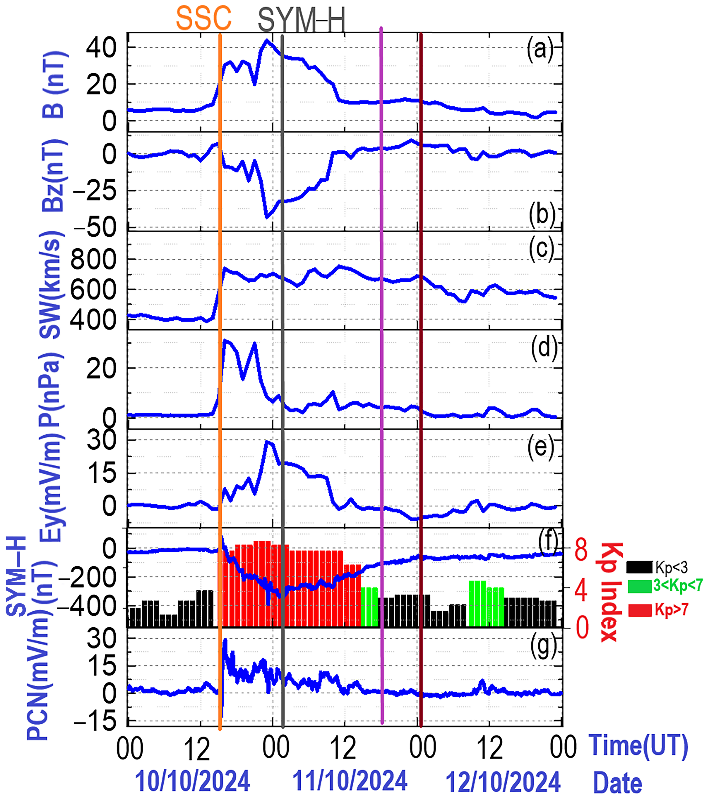
The arrival of this IP shock at Earth’s magnetosphere triggered a Sudden Storm Commencement (SSC) at 15:16 UT on 10 October, as shown in Figure 2a–g as an orange line. At the time of SSC, the 1 min SYM—H index (equivalent to the hourly Dst index) spiked from 11 nT to 78 nT (Figure 2f), a signature of intensified magnetopause current. Immediately afterwards, the SYM—H index began to fall sharply, indicating the onset of the storm’s main phase. This phase continued until the index reached a minimum of −346 nT at 01:46 UT on 11 October, as depicted by the grey line in Figure 2a–g. A gradual recovery followed, with the SYM—H returning to near pre-storm levels by 00:26 UT on 12 October as shown by a brown line. A notable intermediate recovery point occurred around 19:38 UT on 11 October, when the index rose above −100 nT (pink line). Between SSC and 23:14 UT on 10 October, the SYM—H index exhibited notable oscillations, linked to fluctuations in the interplanetary magnetic field Bz component (IMF—Bz). Peaks in SYM—H corresponded to northward (positive) IMF—Bz, indicating a more closed magnetospheric configuration, while decreases aligned with sustained southward (negative) IMF—Bz conditions, favourable for magnetic reconnection and energy input into the magnetosphere.

To further assess geomagnetic activity, we examined the global Kp index (Figure 2f), which peaked at 6+ between 15:00 UT on 10 October to 14:00 UT on 11 October, confirming the severity of the event. The Kp index declined significantly afterwards, marking the storm’s recovery phase.

High-latitude geomagnetic activity was evaluated using the Polar Cap Index for the Northern Hemisphere (PCN), which is calculated from magnetic field variation recorded at the Qaanaaq station in Greenland. PCN data averaged over 15 min intervals are used to detect geomagnetic disturbances in the polar caps caused by the solar wind’s dynamic pressure and orientation of the IMF [21]. As expected, PCN showed a marked increase in response to the CME impact and tracked closely with Kp, particularly when Kp exceeded level 7, indicating enhanced auroral electrojet activity. On 10 October at approximately 15:00 UT, coinciding with the SSC, solar wind speed jumped sharply from 409 km/s to 740 km/s (Figure 2c), confirming the CME’s arrival. At the same time, IMF—Bz turned strongly negative (Figure 2b), while the total magnetic field strength (IMF—B) showed multiple successive increases, consistent with the passage of a complex CME structure. These conditions facilitated prolonged and intense dayside magnetic reconnection at the magnetopause, enabling massive energy transfer into Earth’s magnetosphere. After 00:30 UT on 12 October, IMF—Bz returned to near-zero, and IMF—B weakened to about 4 nT, signalling the end of the storm’s active phase. The long duration and sustained southward orientation of IMF—Bz was a consequence of one of the most geoeffective geomagnetic storms in the recent solar cycle.

4. Results

4.1. Spatio-Temporal Variations in the Ionospheric Characteristics

This section presents a global analysis of the ionospheric response to the geomagnetic storm that occurred on 10–11 October, with particular attention to Hemispheric asymmetries. The analysis focuses on two key ionospheric characteristics: foF2 and hmF2. To capture storm-time variations in these characteristics, we employed Ne profiles obtained from the COSMIC—2 RO satellite constellation. This constellation provides high-resolution coverage up to ±45° geographic latitude, making it particularly suitable for examining ionospheric dynamics in equatorial and low- to midlatitude regions. 9 October, characterized by relatively quiet geomagnetic conditions, was selected as the reference day for comparison of ionospheric characteristics.

Figure 3a–h and Figure 4a–h illustrate the spatial and temporal evolution of foF2 and hmF2 over 9–11 October, in 3-h intervals. Each subfigure in Figure 3a–h and Figure 4a–h represents data accumulated over a 3 h period, based on foF2 and hmF2 measurements derived from COSMIC—2 profiles. Prior to 15:00 UT on 10 October, ionospheric conditions remained largely consistent with the quiet-time reference. The SSC, recorded at 15:16 UT, marked the onset of the main phase of the geomagnetic storm (Figure 2). Between 15:00 and 18:00 UT, minimal ionospheric perturbations were observed in both Hemispheres. However, by 18:00–21:00 UT, storm-related signatures began to manifest. On the dayside of the Northern Hemisphere, particularly across the American sector, a significant increase in hmF2 was evident, indicating a substantial uplift of the F-region. Notably, foF2 values in this region remained largely unchanged. In contrast, on the nightside of the Southern Hemisphere—especially over eastern longitudes—foF2 exhibited a marked decrease, while hmF2 simultaneously increased, implying ionospheric uplift coupled with plasma depletion. An absence of foF2 and hmF2 data was observed in the Afro-European sector, highlighted by a red dotted box in Figure 3 and Figure 4. This data gap began early in the storm and persisted through multiple phases.

During the 21:00–24:00 UT interval, foF2 remained relatively stable on a global scale, but hmF2 continued to rise across both Hemispheres’ dayside sectors, with uplifts reaching 150–200 km.

Between 00:00 and 03:00 UT, coinciding with the SYM–H minimum, foF2 decreased significantly over the Southern Hemisphere nighttime sector. Simultaneously, a significant reduction in hmF2 was recorded over the isolated Australian longitudes (marked as “A” in Figure 4). Although storm activity weakened during the subsequent recovery phase, ionospheric disturbances remained pronounced in the Southern Hemisphere until approximately 12:00 UT. Isolated regions, marked as “B” and “C” in Figure 4, also showed severely low hmF2 values during this period. Moreover, the previously noted data gap migrated westward over time—from the Afro-European region to the Atlantic sector, and eventually to the Western Pacific by 18:00 UT on 11 October.

These results underscore several key features of the ionospheric response during the storm. A persistent uplift of the F-region was observed across both Hemispheres during the main and early recovery phases, particularly on the dayside. Meanwhile, foF2 consistently decreased on the nightside, especially in the Southern Hemisphere, indicating enhanced recombination processes and plasma loss. The absence of foF2 and hmF2 measurements during nighttime hours across specific longitudes is particularly notable. From 15:00 to 03:00 UT, these data gaps were observed over the Afro-European sector, later shifting toward the Atlantic and Pacific regions during the recovery phase, before dissipating after 18:00 UT on 11 October. A rational justification for the absence of foF2 and hmF2 values is the occurrence of negative ionospheric storm effects, where significant plasma depletion causes ionization densities to drop below the level required for signal reflection. Such conditions are common during the main and early recovery phases of intense geomagnetic storms, as storm-induced changes in thermospheric composition lead to increased concentrations of molecular species like N₂ and O at F-region altitudes. This enhances recombination processes, resulting in reduced electron densities. Similar global ionospheric responses were also observed during the Mother’s Day 2024 storm, as reported by Paul et al. (2025) [5]. However, the decrease in hmF2 observed during the recovery phase of the October storm, particularly over the Southern Hemisphere’s nighttime sector, appears to be a distinctive feature compared to the May 2024 event. The markings “A–C” in Figure 4 are spatially limited primarily due to the observational constraints of the COSMIC—2 mission. The data consist of discrete COSMIC—2 profiles that are sparsely distributed along satellite ground tracks and aggregated over a 3 h interval. Consequently, only areas with sufficient profile density and clearly observed apparent hmF2 reductions could be highlighted. While this representation may not capture the full spatial extent or finer-scale variability of the phenomenon, it still provides a meaningful approximation of localized storm-time effects in the F-region ionosphere.

A plausible explanation for these apparent hmF2 drops is the development of G-conditions, wherein the foF2 drops below the F1 layer (foF1) as a result of pronounced F-region uplift combined with a reduction in Ne. A G-condition in the ionospheric F-region occurs when the critical frequency of the F2 layer becomes equal to or less than that of the F1 layer, i.e., foF2 ≤ foF1, where foF2 and foF1 represent the critical frequencies of the F2 and F1 layers, respectively. Studies [6,7] have shown that G-conditions typically arise due to changes in thermospheric parameters—such as density, composition, temperature, and wind velocity—which primarily reduce foF2, while foF1 remains largely unaffected. These reductions in foF2 are characteristic of the negative phase of an ionospheric storm, and the link between this phase and thermospheric disturbances is widely recognized. This mechanism is frequently associated with intense geomagnetic disturbances and is supported here by the clear evidence of hmF2 elevation shown in Figure 4a–h. In the case of COSMIC—2 observations, the F2 peak may rise above the maximum detection altitude of the COSMIC—2 RO, making it inaccessible. As a result, the observed hmF2 values under such conditions do not represent the true F2 peak height but instead reflect the height of the underlying F1 layer, which the retrieval algorithm misidentifies as hmF2. This misinterpretation leads to an apparent reduction in the peak height. G-conditions were also observed during the September 2017 geomagnetic storm over European midlatitudes [7]. Similarly, Paul et al. (2025) [5] documented G-conditions in European midlatitude ionograms during the 2024 Mother’s Day superstorm, attributing this to abrupt extreme F-region uplift. Their subsequent global study further confirmed the widespread occurrence of G-conditions during that storm.

To investigate the significant drop in hmF2—particularly over certain Southern Hemisphere nighttime sectors during the recovery phase—individual COSMIC—2 Ne profiles were examined. Figure 5a–h displays eight satellite passes between 00:00 and 03:00 UT, each confirming the presence of G-conditions, characterized by foF1 exceeding foF2 and the F1 layer misinterpreted as the Ne peak. This pattern was further validated by Figure 6a–h and Figure 7a–h, covering the 03:00–06:00 UT and 09:00–12:00 UT intervals, respectively, which revealed similar G-condition signatures. The consistency of these observations across multiple satellite passes strongly supports the conclusion that G-conditions were widespread during the storm’s main and early recovery phases.

We also examined vertical and horizontal ion drift velocities using data from three Digisonde stations located in both Hemispheres. Figure 8a–c presents the variations in vertical (Vz), north—south (Vnorth), and east—west (Veast) ion drifts throughout the storm period. At Lualualei, situated in the nightside equatorial sector of the Northern Hemisphere over the Pacific Ocean, a strong downward drift of approximately −153 m/s was observed immediately following the SSC, indicating a pronounced negative storm effect in the nightside equatorial ionosphere. Although vertical drifts at this station showed considerable variability during the main phase, horizontal drift velocities remained relatively stable except during periods of heightened geomagnetic activity. Around 22:00 UT, a sharp southward drift of ~480 m/s was recorded, followed by a high northward drift of ~430 m/s at 23:00 UT. These alternating drifts suggest complex electrodynamic processes involving the equatorward expansion of the polar ionosphere and the poleward extension of equatorial plasma. Unfortunately, no drift data were available at Lualualei during the storm recovery phase.

At Eglin, located in the dayside equatorial sector of the Northern Hemisphere, an upward drift was recorded near the SYM–H minimum, which may signify the onset of G-conditions—when foF2 drops below foF1 due to plasma depletion and F-layer uplift. During the main and recovery phases, Eglin exhibited highly variable horizontal drift patterns, including northeastward drifts of ~700 m/s by 23:27 UT, a shift to northwestward drifts of over 500 m/s at 00:57 UT, and a further intensification to ~900 m/s by 01:42 UT, before settling into a predominantly westward flow. These rapid and large-amplitude changes in drift direction and magnitude reflect the dynamic response of the dayside ionosphere to storm-time electric field penetration and thermospheric wind modification.

In the Southern Hemisphere, over Ascension Island, located in the equatorial sector, intense upward (~170 m/s) and southwestward (~1000 m/s) drifts were observed during the storm’s main phase. These signatures are consistent with a poleward expansion of the EIA, likely driven by prompt penetration electric fields (PPEFs). During the storm’s recovery phase, upward and southwestward drifts remained dominant, aligning with findings from Picanço et al. (2025) [18], who reported similar drift patterns at Ascension Island during this period.

Picanço et al. (2025) [18] further examined equatorial ionospheric behaviour during the storm by comparing observations from São Luís and Jicamarca stations. Their analysis revealed significant discrepancies in F-region uplift patterns due to the influence of PPEFs. At Jicamarca, an under-shielding electric field event around the time of the post-sunset PRE led to a maximum F-region uplift of nearly 700 km. In contrast, São Luís recorded a storm-induced uplift of ~560 km occurring approximately three hours earlier than the usual PRE timing. Additionally, they observed a second uplift event driven by DDEFs, with F-region heights reaching ~410 km over São Luís around 07:00 UT and ~450 km over Jicamarca at 08:00 UT on 11 October. This second uplift coincided with intensifying auroral oscillations, highlighting a complex and possibly coupled electrodynamic response between high-latitude auroral processes and equatorial ionospheric dynamics.

To assess the impact of the geomagnetic storm on thermospheric composition, we compared the latitudinal and longitudinal distribution of the [O/N₂] ratio under both quiet and disturbed conditions using data from the GUVI. This comparison is illustrated in Figure 9a–d. Under quiet conditions, as shown in Figure 9a, the [O/N₂] ratio appears relatively uniform across all latitudes throughout the day. This consistency indicates efficient meridional and zonal transport of neutral particles, leading to a balanced composition and enhanced daytime recombination, with minimal spatial variability or lags in the neutral response. However, during disturbed conditions on 10–11 October, the global [O/N₂] distribution, presented in Figure 9b,c, reveals significant deviations from the quiet-time pattern. Notably, large fluctuations in the [O/N₂] ratio were observed over the equatorial and polar regions, indicating strong thermospheric disturbance. These fluctuations are likely the result of enhanced vertical and horizontal neutral wind circulation driven by geomagnetic forcing, which redistributes atomic oxygen and molecular nitrogen unevenly across latitudes. In contrast, the midlatitude region displayed relatively subdued [O/N₂] variability, suggesting that longitudinal inhomogeneities in thermospheric composition were less pronounced in these regions during the storm. This indicates a more stable thermospheric response at midlatitude compared to the more dynamically perturbed equatorial and polar sectors, which are more directly influenced by storm-driven energy inputs and magnetosphere—ionosphere—thermosphere coupling process.

4.2. Storm Effects on Swarm Observation

In the previous section, the analysis of storm-induced changes in foF2 and hmF2 was limited to ±45° geographic latitude due to the restricted latitudinal coverage of COSMIC–2. To expand this latitude scope and gain a more complete picture of the global ionospheric response, the current section examines in situ Ne measurements from Swarm satellites A and B during the October 2024 geomagnetic storm. While Swarm data have been extensively used to study the May 2024 Mother’s Day superstorm, a detailed global study of Swarm Ne response to the October event has not yet been reported. Xia et al. (2025) [22] investigated field-aligned currents (FACs) and polar electrojet (PEJ) activity during this storm, but their analysis was confined to the polar ionosphere.

To address this gap, we analyzed Swarm A and B Ne data for the interval from 15:00 UT on 10 October to 21:00 UT on 11 October. This time frame was selected based on both the SYM–H index (Figure 2) and foF2/hmF2 variation (Figure 3 and Figure 4), which indicate that significant storm activity diminished after ~21:00 UT on 11 October. The comparison was based on data from 5,6 October, which represents geomagnetically quiet conditions. The results are presented in Figure 10a–t and Figure 11a–t, where each set of four panels per time window displays (1) Swarm Ne for quiet conditions, (2) storm-time Ne, (3) Madrigal global TEC maps under quiet conditions, and (4) corresponding storm-time TEC maps.

To assess storm-induced global ionospheric variations, it is essential to first characterize the typical behaviour of the ionosphere under geomagnetically quiet conditions. For this purpose, we analyze ionospheric observations from 15:00 UT on 5 October to 21:00 UT on 6 October, as illustrated in Figure 10 and Figure 11. This study primarily aims to examine the potential poleward expansion of the EIA and the equatorward extension of the polar ionosphere, with particular focus on the EIA dynamics and polar ionospheric responses. Swarm A, orbiting at a lower altitude than Swarm B, exhibits more pronounced EIA features along its trajectory. Between 15:00 and 18:00 UT on 5 October, well-defined EIA crests are observed within ±15° magnetic latitude across the European-African sector, where the geographic and geomagnetic equators are closely aligned. In the South American sector, Swarm B also detects a significant crest near −15°N, indicative of enhanced equatorial fountain effects. As the observation period progresses, both Swarm A and B detect EIA signatures over western longitudes. Over South America, EIA crests recorded by Swarm A between 21:00 UT on 5 October and 03:00 UT on 6 October extend from 5°N to −30°N following the geomagnetic equator. During the same interval, Swarm B observes increased perturbations across equatorial regions (±15° latitude), particularly over the Pacific sector. Between 03:00 and 06:00 UT, Swarm A continues to record westward EIA development confined within ±15° latitude, while Swarm B detects heightened ionospheric disturbances over the Asian region, suggesting intensified fountain effects at higher altitudes. From 06:00 to 15:00 UT on 6 October, the EIA observed by Swarm A remains concentrated within ±15° latitudes over the Asian-Australian sectors. After 15:00 UT on 6 October, ionospheric behaviour returns to patterns similar to those observed on 5 October.

During the initial hours of the storm, Swarm A and B did not show significant global Ne depletions immediately following the SSC at 15:16 UT. However, as the main phase of the storm developed, Swarm A observed a notable Ne depletion (~3.2 × 10⁶ electrons/cc) across the Afro-European sector and increased variability over the Pacific. Swarm B recorded ionospheric perturbations over both North and South American sectors. When compared to quiet-day Swarm observations on 5 October, storm-time data clearly demonstrated an expansion of the EIA, particularly over the Southern Hemisphere of the Afro-European and American longitudes. Picanço et al. (2025) [18] reported a similar expansion between longitudes −50° and −130° around 18:00 UT, which corresponds well with our findings in Figure 10f. Notably, over Africa, Swarm B detected a sharp Ne depletion, indicative of strong upward plasma drift, validated by a pronounced depletion in the corresponding Madrigal TEC map at 21:40 UT (Figure 10l). These results reinforce findings from Figure 4, an F-region uplift—now confirmed by Swarm data.

Between 00:00 and 06:00 UT on 11 October, the storm reached its peak intensity. During this period, Swarm B data revealed that the EIA expanded from ~45°N to ~60°S, especially on the dayside, with more limited expansion on the nightside. Plasma uplift was strongest between 30°N and 45°S, particularly evident in Swarm B (Figure 10n). At 00:20 UT on 11 October, TEC maps from Madrigal revealed a distorted “C”-shaped EIA crest in both Hemispheres (Figure 10p), similar to observations reported by Picanço et al. (2025) [18], who attributed this reversed C-shaped structure to enhanced vertical and zonal drifts, driving the expansion of polar irregularities to midlatitudes and merging with equatorward-propagating EPB structures. Between 03:00 and 06:00 UT, poleward expansion of the EIA gradually subsided on the dayside, while plasma uplift remained active from 45°N to 45°S, especially in the nightside equatorial sector. This continued uplift is consistent with higher hmF2 values observed in Figure 4 over the African and American longitude sectors.

Figure 11a–t extends this analysis to 06:00–21:00 UT on 11 October, capturing the storm’s recovery phase. From 06:00 to 09:00 UT, the Northern Hemisphere exhibited an expansion of the nightside EIA from 30°N to 45°N, while the Southern Hemisphere displayed a contraction of the EIA. Simultaneously, Swarm B detected a significant dayside Ne depletion over the American and Pacific sectors, aligning with earlier hmF2 observations (Figure 4c). From 09:00 to 15:00 UT, this pattern persisted—nightside contraction in the South and dayside expansion remained evident but weakened. Notably, between 12:00 and 15:00 UT, Ne depletion was sustained over the equatorial dayside Southern Hemisphere, confirmed by Swarm B (Figure 11j). Picanço et al. (2025) [18] observed similar features, attributing them to a second uplift phase driven by DDEFs, with F-region heights reaching ~410 km over São Luís and ~450 km over Jicamarca between 08:00 and 09:00 UT. This timing also coincided with intensified auroral activity, indicating electrodynamic coupling between polar and equatorial ionospheric regions.

By 15:00 UT, Swarm A data indicated minimal storm-time expansion, while Swarm B continued to show moderate depletion over the Southern Hemisphere dayside. After 18:00 UT, Ne values from both Swarm A and B returned to near-quiet levels, marking the end of significant ionospheric disturbance.

Overall, the analysis underscores the significant role of storm-driven PPEFs in expanding the EIA and driving vertical plasma transport. Swarm A and B data, supported by global TEC maps from Madrigal, confirm that the topside ionosphere experienced substantial restructuring, particularly during the PRE period. The emergence of two distinct EIA crests in Swarm Ne further supports the influence of PPEF-driven vertical drift, consistent with results reported by Paul et al. (2025) [6]. Additionally, the study highlights clear Hemispheric asymmetries in the storm-time ionospheric response, manifested in plasma circulation patterns, thermospheric wind variations, TEC distributions, and magnetic field perturbations. These findings are consistent with earlier research by Laundal et al. (2016) [23], who emphasized the fundamental role of Inter-Hemispheric differences in shaping space weather responses during geomagnetic storms.

4.3. Large-Scale Travelling Ionospheric Disturbances

LSTIDs are manifestations of GWs and are frequently observed across the global ionosphere. During geomagnetic storms, the probability of LSTID formation and propagation increases significantly due to intensified energy input into the upper atmosphere [5,7]. TEC perturbations are commonly used to detect and analyze TID behaviour in space weather studies. Borries et al. (2010) [24] reported such storm-time LSTID signatures in the European sector. In this study, we examined LSTID activity during the main phase of the October 2024 geomagnetic storm, particularly from 15:00 UT on 10 October to 02:30 UT on 11 October—a period considered optimal for LSTID generation [24]. To do so, we analyzed global dTEC maps, as described in Section 2. While we were limited to visual identification of propagation direction due to the data format, which precludes estimation of LSTID periodicity, wavelength, or speed, the methodology for generating and interpreting these maps is well established in Otsuka et al. (2002) [20]. Given the spatial density of GNSS stations, this analysis focuses on the Northern Hemisphere, particularly Europe, Japan, and North America.

Figure 12, Figure 13, Figure 14, Figure 15, Figure 16 and Figure 17 present the evolution of LSTID activity across the Northern Hemisphere during the storm’s main phase. Following the SSC at 15:16 UT, initial LSTID signatures were detected over both the European (marked by the red circle) and Japanese (blue circle) sectors, as shown in Figure 12a–d. During the 15:20–15:50 UT interval, dTEC fluctuations reached ~4 TECU over Europe and ~5 TECU over Japan. LSTID propagation directions suggested southwestward movement over Europe and possible equatorward expansion of the polar ionosphere, consistent with findings by Picanço et al. (2025) [18].

As the storm intensified, LSTID activity became more widespread. Figure 13a–d displays dTEC patterns from 17:00 to 17:40 UT. LSTID signatures extended to the North American sector, marked by the green circle. In Europe, LSTIDs were evident over the polar latitudes (60–70°N) propagating northeastward, while midlatitude LSTIDs appeared to move from southeast to northwest. In Japan, southward-propagating LSTIDs were detected, especially during 17:00–17:10 UT. The North American region also showed signs of poleward EIA expansion, particularly between 17:00 and 17:20 UT.

During 19:10–19:50 UT (Figure 14a–d), LSTIDs intensified further. The European polar region exhibited an east—west structured plasma pattern, while Japan showed southwest-to-northeastward-propagating LSTIDs that intensified toward the end of the interval. In North America, a dTEC depletion at 19:10 UT shifted northeastward with decreasing fluctuation magnitude—again suggesting poleward EIA expansion.

At the storm’s peak, Figure 15a–d shows clearer LSTID patterns, particularly over North America, where northeast-to-southwest-propagating LSTIDs dominated. The European polar region recorded high dTEC fluctuations, while the western midlatitude sector experienced sharp depletions. Pierrard et al. (2025) [17] linked these ionization changes to intense F-region perturbations, amplified by the plasmaspheric effect on VTEC.

From 22:00 to 00:00 UT, as the storm approached maximum intensity (Figure 16), dTEC maps revealed widespread LSTID activity throughout the Northern Hemisphere. Over Europe, LSTIDs propagated from northeast to southwest in the polar region and expanded toward midlatitude by 23:40 UT. Midlatitude LSTIDs moved northeastward until they were surpassed by polar-origin depletions. Japan registered LSTIDs moving from northeast to southwest, which weakened by 23:40 UT following the arrival of significant depletions. In North America, the LSTID signature was clearly observed with a northeast-to-southwest orientation across much of the region.

At the peak of the storm, as the SYM—H index reached its minimum (~01:46 UT), LSTID activity was observed across all three sectors. Figure 17a–h shows dTEC maps from 01:20 to 02:30 UT. In Europe, midlatitude regions recorded strong northwest-to-southeast LSTIDs, which intensified over time. The polar ionosphere exhibited intense dTEC depletion, while Japan displayed a contrasting trend. Although northeast-to-southwest LSTID traces were observed at 01:20 UT, these weakened as the SYM—H reached its minimum and were nearly undetectable by 01:50 UT. Around 02:10 UT, LSTID activity intensified. North America showed strong LSTID traces, again oriented southwestward, which strengthened with decreasing SYM—H and subsided during the recovery phase.

These observations align with those reported by Oikonomou et al. (2022) [7] during the September 2017 storm and Paul et al. (2025) [5] during the May 2024 superstorm. Borries et al. (2010) [24] found a strong correlation between auroral electrojet (AE) activity and LSTID amplitudes. Our results reinforce the idea that storm-time conditions—intensified thermospheric westward wind—enhance GW generation, which in turn drives LSTID propagation globally. The coincidence of a strong electric field and enhanced thermospheric circulation—both components of magnetosphere–ionosphere–thermosphere coupling—further suggests that LSTIDs during intense geomagnetic storms are linked not only to GW dynamics but also to electrodynamic plasma instabilities. The storm-time electric field may act as a trigger for plasma instabilities with rapid growth rates, ultimately contributing to TID generation and evolution, as proposed by Zhang et al. (2022) [25].

Although the global dTEC maps mentioned above provide dense coverage over the Northern Hemisphere, their resolution is significantly lower in the Southern Hemisphere, particularly over the Asian sector. To investigate the ionospheric response to the geomagnetic storm in the Southeast Asian region, we utilized ROTI data from the Ina-CORS GNSS network. Figure 18a–c display the storm-time ROTI maps for this region. Figure 18a shows the ROTI distribution during the initial phase of the storm, specifically from 15:00 to 17:00 UT on 10 October. It is important to note that the local time (LT) in this region is approximately 7.5 h ahead of UT, placing this interval during nighttime conditions. As seen in Figure 18a, significant ROTI perturbations exceeding 1 TECU/min are evident in the Southern Hemisphere sector. These irregularities began to emerge around 15:15 UT, intensified by 15:40 UT, and started to diminish after 16:45 UT. A distinct southwestward propagation of these structures can be observed. Similar findings were reported by Abadi et al. (2025) [26] during the Mother’s Day 2024 superstorm, where enhanced ROTI values were observed during post-sunset hours across Southern Australia. They attributed these enhancements to either the equatorward expansion of auroral activity or the influence of the midlatitude trough. According to their study, the irregularities initially appeared near 150°E at around 12:50 UT, and subsequently propagated northwestward and southwestward over the Japanese and Australian sectors, respectively. As the storm evolved, these equatorial irregularities diminished. During the recovery phase, at approximately 01:50 UT, weak ROTI perturbations (~0.4 TECU/min) were observed near the geographic equator, as shown in Figure 18b (highlighted by the red circle), followed by another brief occurrence between 03:05 and 03:25 UT, depicted in Figure 18c. These later disturbances were notably weaker in intensity.

5. Discussion

The present study focuses on the storm-induced global ionospheric response to the October 2024 storm, with the following impacts highlighted in Section 4.

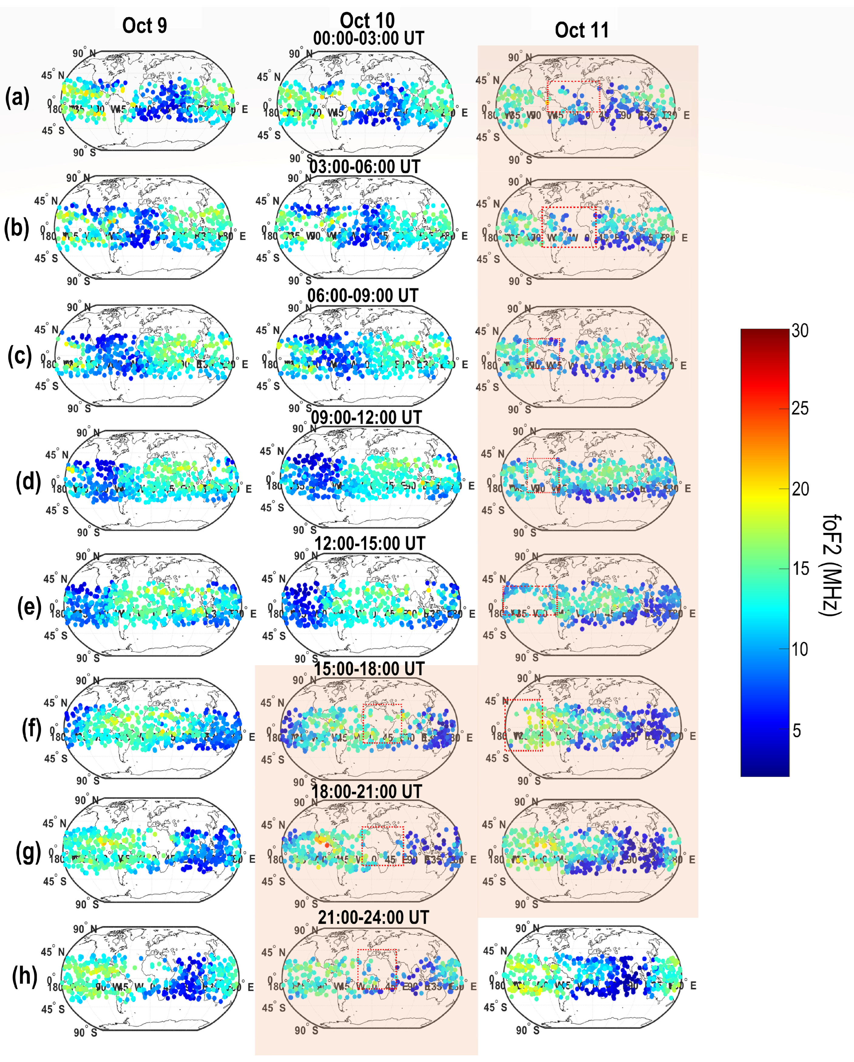
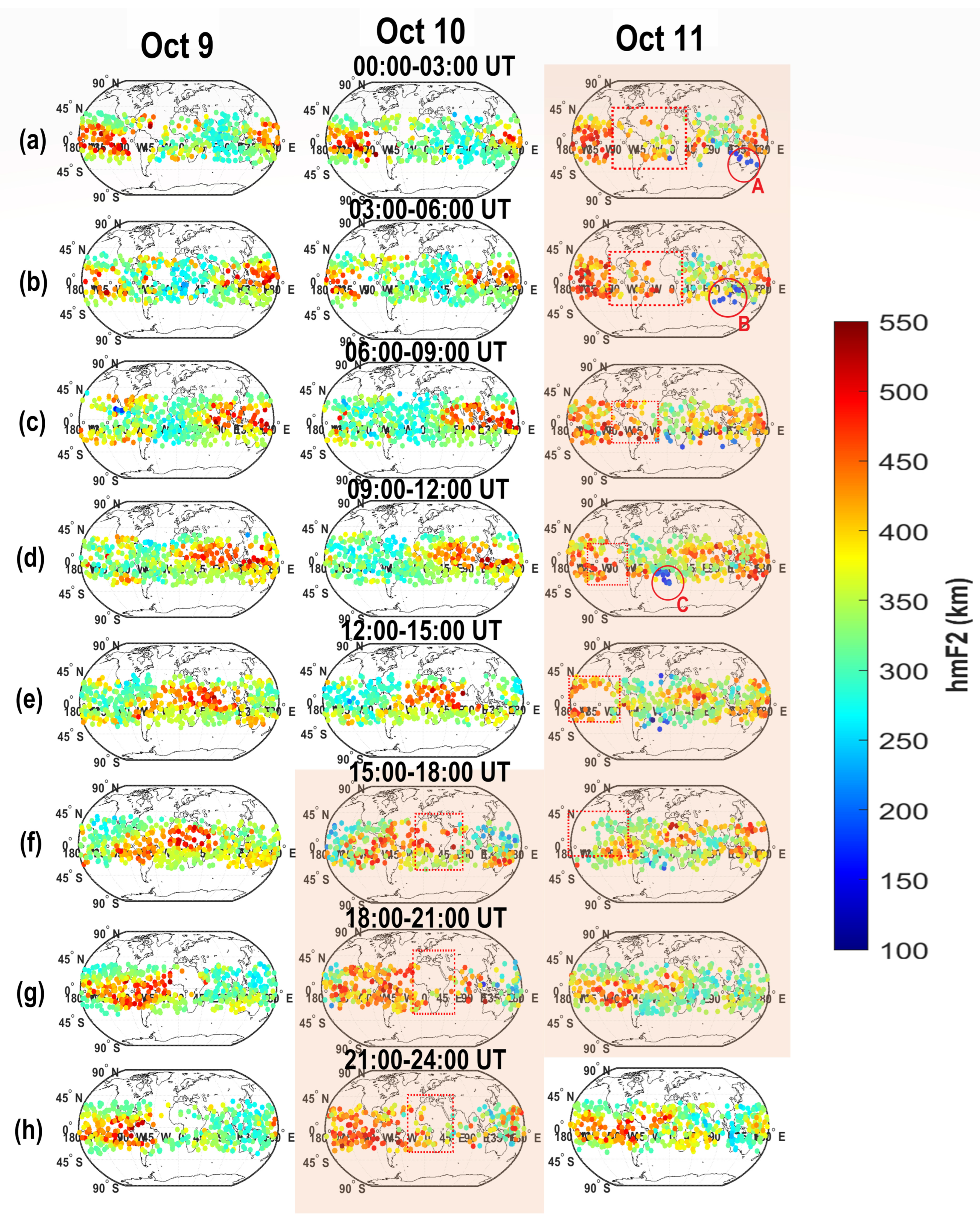
A storm-induced F-region uplift manifested as an increase in hmF2, observed on the dayside in both Hemispheres. This enhancement occurred while foF2 remained largely stable, except in the American longitude sector during the storm’s early active phase. Conversely, a marked decrease in foF2, accompanied by uplift of the F-region, was detected on the nightside of the Southern Hemisphere during both the initial and main phases of the storm, as shown in Figure 3a–h and Figure 4a–h. Certain nighttime longitude sectors displayed missing foF2 and hmF2 values during the storm period, highlighted by red rectangles in Figure 3a–h and Figure 4a–h, a pattern also noted during the Mother’s Day 2024 superstorm [6]. During the main and early recovery phases, extremely low hmF2 values were recorded over some isolated regions in the Southern Hemisphere’s nightside sector, as indicated by regions A, B, and C in Figure 4. 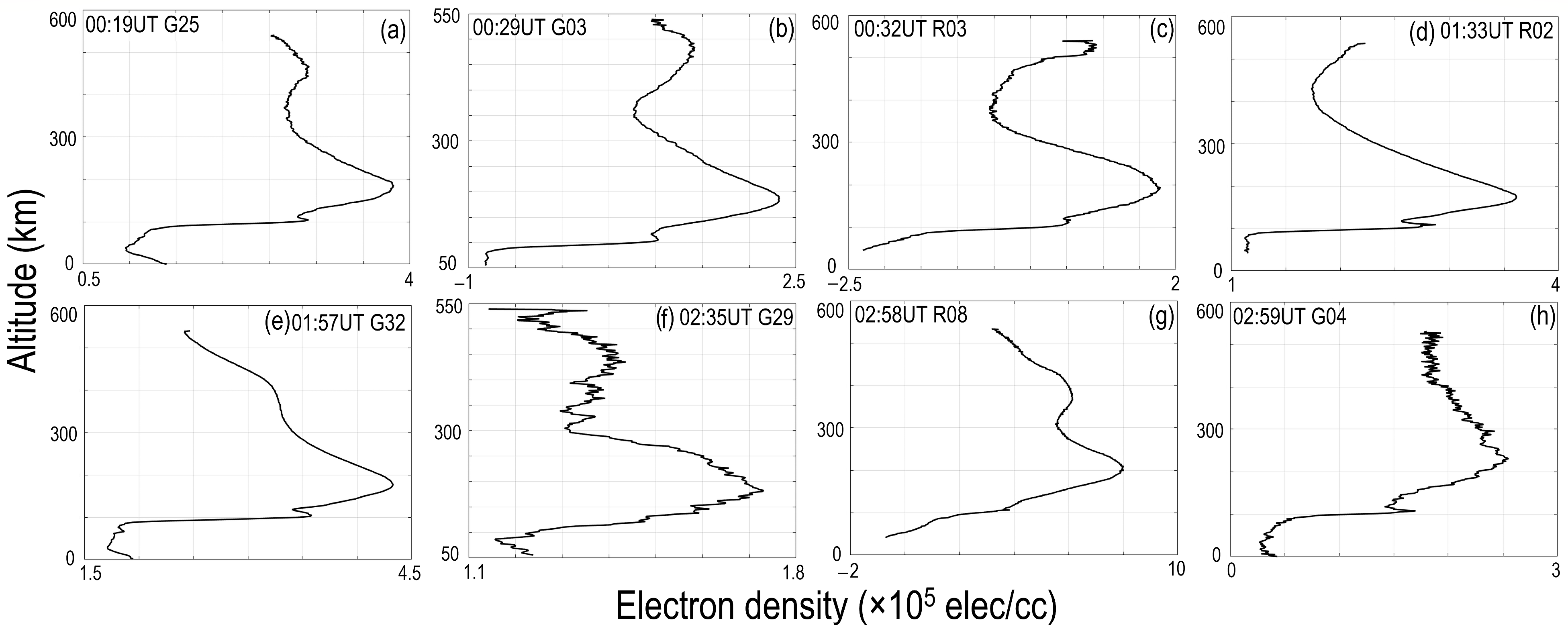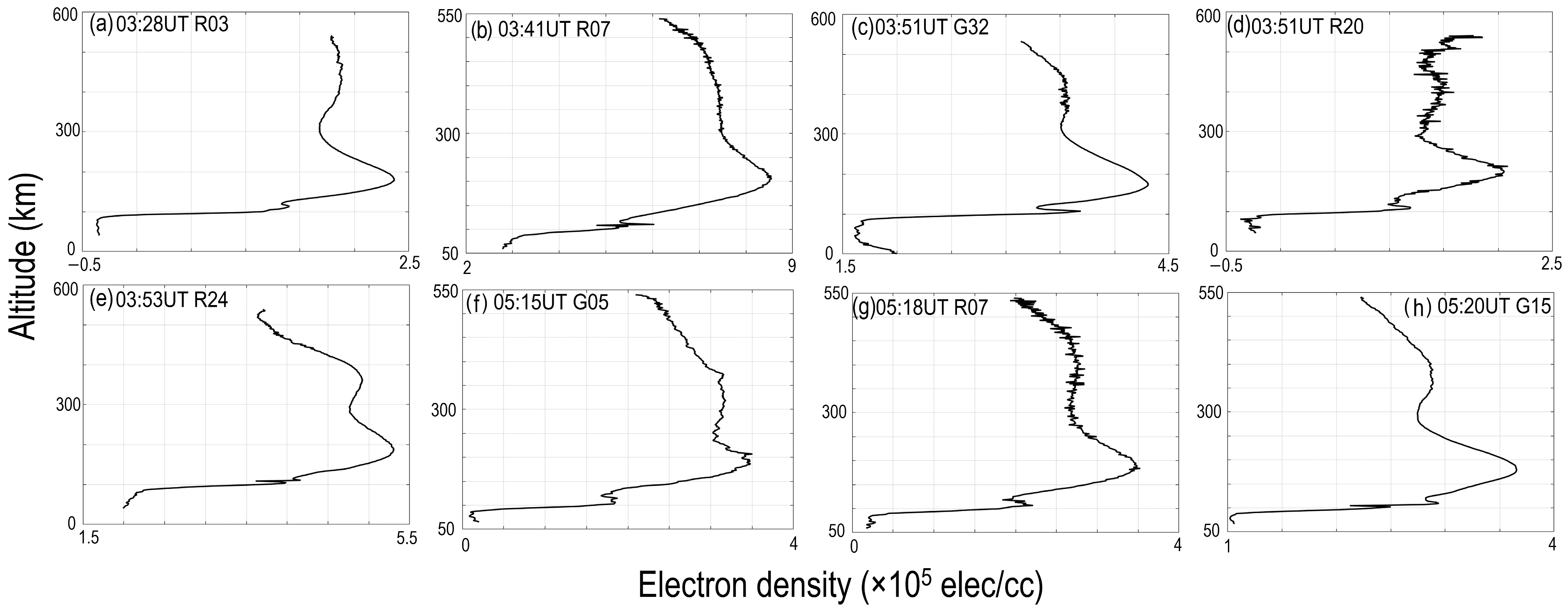Section 4 attributes these to G-conditions, which are further illustrated in Figure 5a–h, Figure 6a–h and Figure 7a–h, where COSMIC Ne profiles show foF1 exceeding foF2 and the F1 layer emerging as the Ne peak—most evident between 00:00 and 12:00 UT.

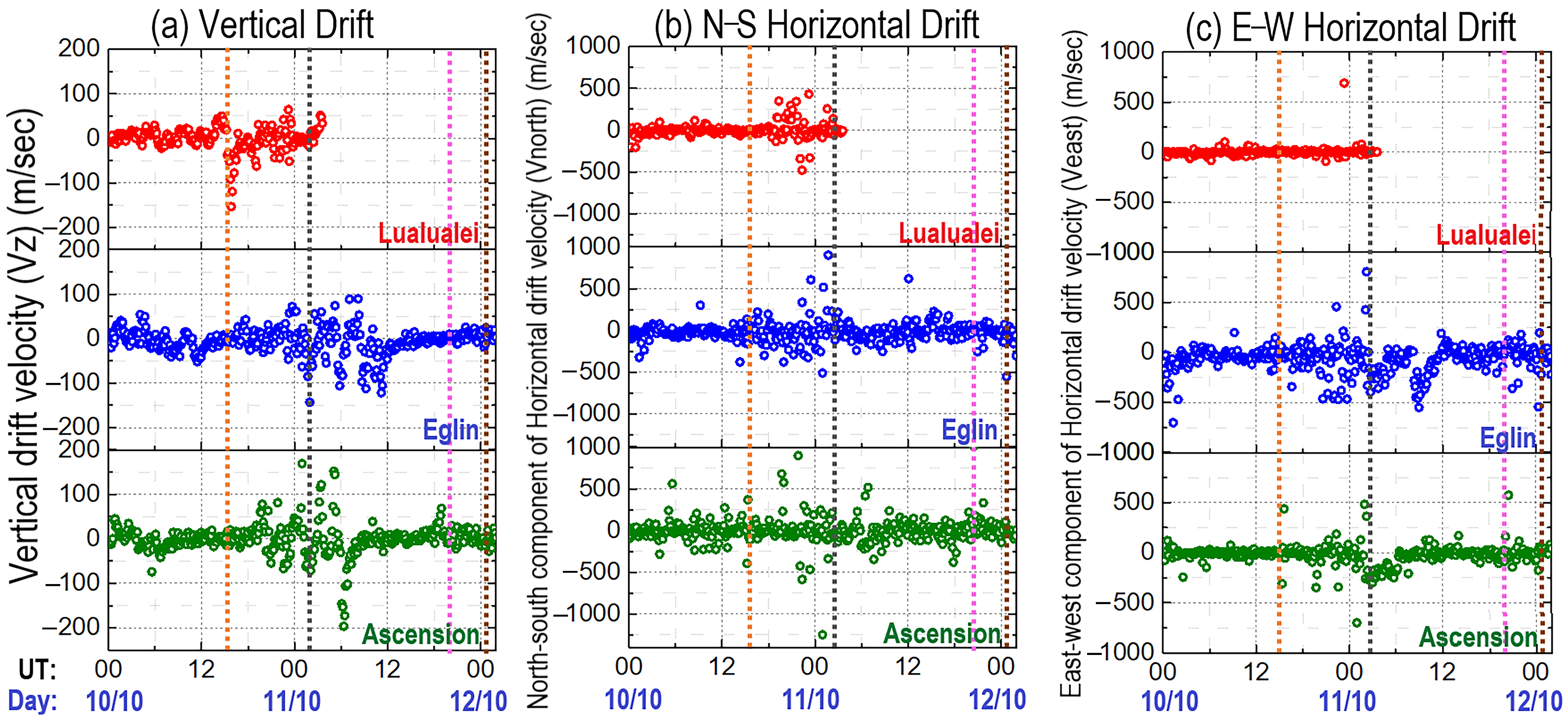
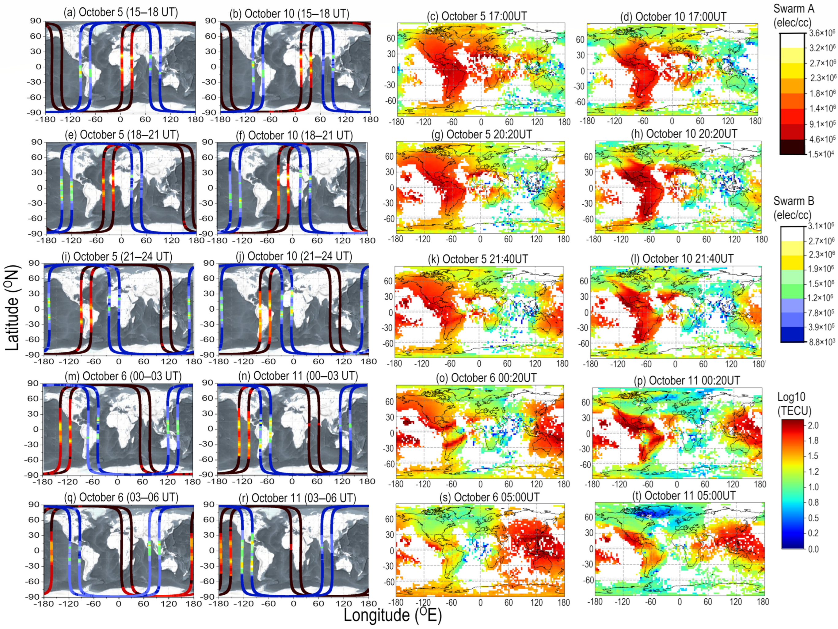
The substantial F-region uplift during the storm is corroborated by strong vertical plasma drifts recorded at Eglin and Lualualei in the Northern Hemisphere and Ascension Island in the Southern Hemisphere (Figure 8a). Swarm B data also indicated considerable Ne depletion over the dayside (Figure 10), implying that the F2 peak was over the observational range of COSMIC—2.

The ionospheric response at high latitudes is initially driven by Joule heating, which raises upper thermospheric temperatures and accelerates neutral wind via ion drag. This heating initiates a global wind surge from polar to lower latitudes and into the opposite Hemisphere, often manifesting as a large-scale GW. This circulation creates midlatitude wind patterns, with GW and background wind representing complementary aspects of the same process. The surge, which favours the nightside and magnetically conjugate regions, is UT-dependent. Meanwhile, the thermospheric composition bulge—characterized by enhanced molecular nitrogen [N₂] and reduced atomic oxygen [O]—is shaped by both background and storm-driven winds, not merely Earth’s rotation. During geomagnetic storms, storm-time winds determine its location, while background winds modulate its diurnal variation during recovery.

The rise in hmF2 is mainly due to equatorward wind that uplifts the F-region, while the drop in foF2, especially in sunlit areas, is tied to increased molecular nitrogen enhancing recombination and reducing Ne. These effects vary with local time and longitude, reflecting the spatial complexity of storm-time ionospheric responses. Increases in foF2—“positive phases”—typically occur on the dayside due to ionospheric uplift and equatorward plasma transport, known as the “dayside ionospheric superfountain.” These are driven by strong southward IMF, which induces a dawn-to-dusk electric field that promotes plasma convection. Though direct measurements are limited, models by Vasyliūnas (1969) [27] and Fuller—Rowell et al. (1994) [28] support these mechanisms. On the nightside, low background ionization obscures positive phases, but dusk-time uplift can extend their effects. Negative phases, in contrast, are linked to the movement of the composition bulge and intensified thermospheric changes. This uplift matches the model proposed by Fuller—Rowell et al. (1994) [28], where meridional winds lift plasma and alter the composition. Global divergent winds also induce upwelling and redistribution of thermospheric species. Additional uplift may result from the equatorward expansion of the polar ionosphere and poleward EIA movement. Picanço et al. (2025) [18] noted polar irregularities reaching ~45° magnetic latitude and asymmetrical EPB behaviour over South America—confined to the equator in São Luís but extending to midlatitudes—merging with auroral structures. This likely caused a strong F-region uplift apparent on ionograms, as supported by Paul et al. (2025) [6] and Figure 4. Strong F-region uplift was observed globally during both the storm’s main and recovery phases (Figure 4a–h), with vertical drift speeds exceeding 100 m/s (Figure 8a). The most intense uplift occurred over Ascension Island, accompanied by enhanced hmF2 at other Southern Hemisphere stations. These effects are attributed to PPEFs driven by southward IMF—Bz and increased Ey electric field. PPEFs can reach the ionosphere at 5–10% of the upstream field strength [29]. As per Vasyliūnas (1969) [26], such electric fields result from the solar wind–polar cap interactions, producing eastward PPEFs and upward E × B drift. Around 16:00 UT on October 10, IMF—Bz dropped from 6.8 nT to ~−8.9 nT, sustaining the uplift. During recovery, a positive IMF—Bz-initiated DDEF gradually shifts ionospheric dynamics. As Blanc and Richmond (1980) [30] explained, auroral heating triggers equatorward wind, forming Hadley-like circulation and reversing quiet-time electric patterns. The combined effect of DDEFs and PPEFs explains the widespread F-region uplift during the October 2024 storm.

Throughout 10–11 October, negative ionospheric storm effects were evident on the nightside of the Southern Hemisphere, whereas on the dayside, particularly during the storm’s active and recovery stages, elevated F-trace heights occurred without a significant increase in foF2. This suggests ionospheric uplift without corresponding Ne enhancement at COSMIC—2 sampling altitudes. Interestingly, Pierrard et al. (2025) [17] noted a slight foF2 increase over midlatitude Europe during the same storm, in contrast to COSMIC—2 data. This discrepancy may be due to G-conditions, as shown in Figure 5a–h, Figure 6a–h and Figure 7a–h, where the F2 peak may have risen above COSMIC—2’s range, leading to underdetection by satellite instruments but detection by ground-based ionosondes, as reported by Pierrard et al. (2025) [17]. This underscores the need for combined satellite and ground-based observations for a comprehensive understanding of ionospheric storm dynamics.

A clear poleward expansion of the EIA and the associated Hemispheric asymmetries in the ionospheric response to the October 2024 geomagnetic storm were observed. Swarm A in situ Ne measurements (Figure 10a–t and Figure 11a–t) distinctly capture the EIA expansion during the initial and main phases of the storm. These observations are further supported by intensified eastward plasma drift recorded at Eglin and Ascension Island (Figure 8c), highlighting the significant role of electric field dynamics in modulating storm-time plasma transport. While the poleward expansion of the EIA during the October 2024 storm was previously noted by Picanço et al. (2025) [18], the present study offers a more comprehensive, global perspective using Swarm satellite data, capturing the evolution of the EIA across both Hemispheres and multiple longitude sectors.

A key emphasis is placed on the Hemispheric asymmetry of the storm-time ionospheric response, which is attributed to variations in particle precipitation and thermospheric heating. These processes enhance ionization while simultaneously increasing recombination rates, ultimately leading to Ne depletion. This asymmetry is strongly influenced by the day—night variation in Hall conductivity, which modulates the electrodynamic response between Hemispheres. During severe geomagnetic storms, the electric field associated with the equatorial “superfountain” effect becomes substantially more intense than that under quiet conditions. As described by Tsurutani et al. (2008) [29], a strong southward IMF drives a dawn-to-dusk electric field on the dayside, enhancing upward E × B drift and lifting the equatorial F-region to much higher altitudes and latitudes. This vertical transport carries plasma into regions where recombination is slower, allowing solar photoionization to restore plasma densities at lower altitudes and contribute to Ne increase. The result is an intensified and poleward-expanded EIA, with plasma densities enhanced not only in altitude but also in latitude due to continued E × B convection. However, unlike earlier storms, Hemispheric asymmetry during the October 2024 event has not yet been widely reported in the literature, likely due to its recent occurrence and a limited number of processed case studies. Our results, particularly the post-storm hmF2 drop (Figure 4) and asymmetrical EIA behaviour, underscore the need for closer examination of the thermospheric and electrodynamic drivers of this response. In contrast, the Hemispheric asymmetry associated with the May 2024 “Mother’s Day” superstorm has been more extensively documented. For instance, Bojilova et al. (2024) [16] conducted a comprehensive global analysis, highlighting Hemispheric differences at mid and high latitudes arising from enhanced particle precipitation and thermospheric temperature gradients. Their findings also emphasized low-latitude coupling via DDEFs, which modulated the EIA distinctly between Hemispheres. Foster et al. (2024) [12] attributed observed westward and equatorward auroral surges at midlatitudes to low-energy electron precipitation, which induced Hemispherically asymmetric westward plasma drifts. Guo et al. (2024) [31] identified storm-time thermospheric circulation as a key factor in producing east–west asymmetries, adding a longitudinal dimension to Hemispheric divergence. Xu et al. (2013) [32] further linked southern polar heating to longitudinal mass density anomalies, extending to mid- and low latitudes. Aa et al. (2012) [33] likewise reported that enhanced Joule heating near the southern magnetic pole (~140°E) can propagate thermospheric effects across the equator, ultimately affecting the low-latitude ionosphere and producing asymmetric enhancements in [O/N₂] ratios.

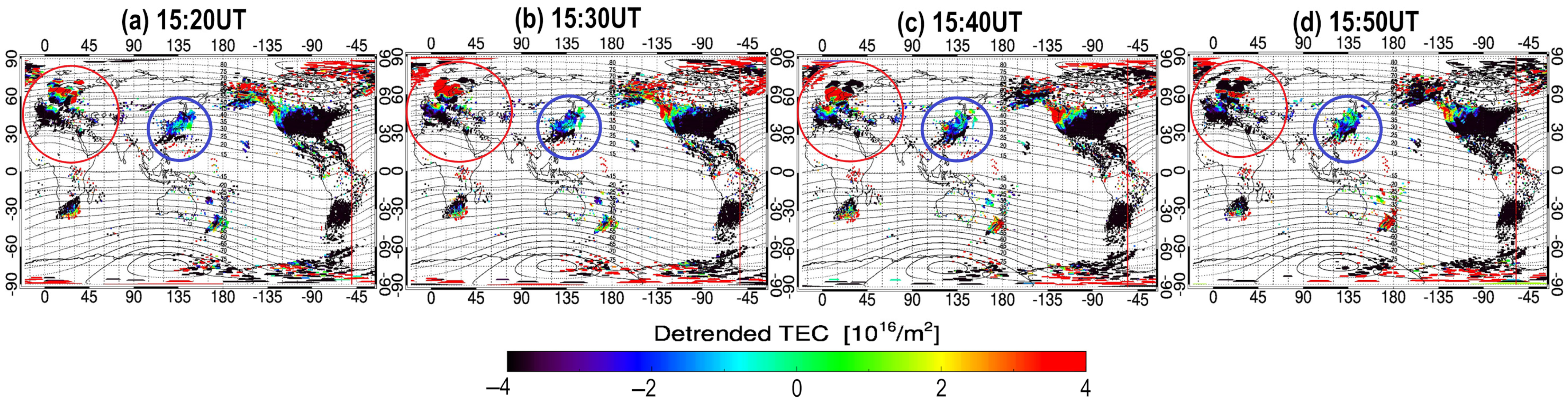
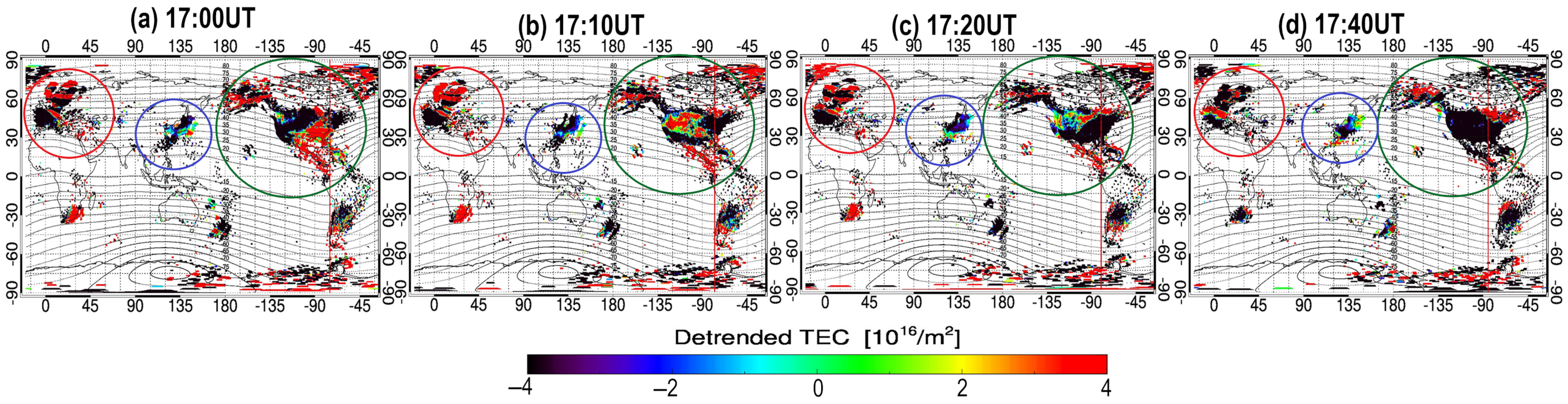
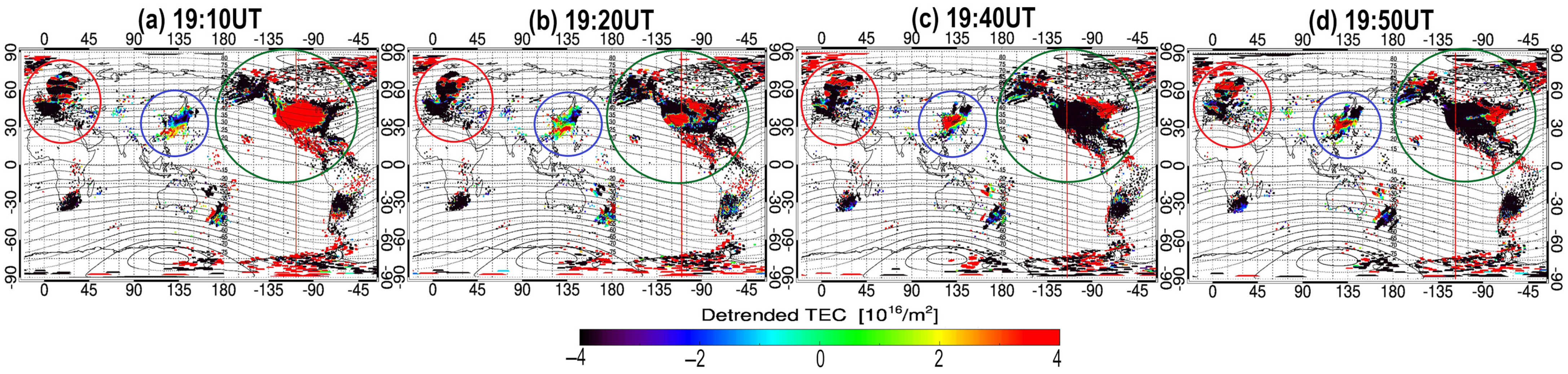
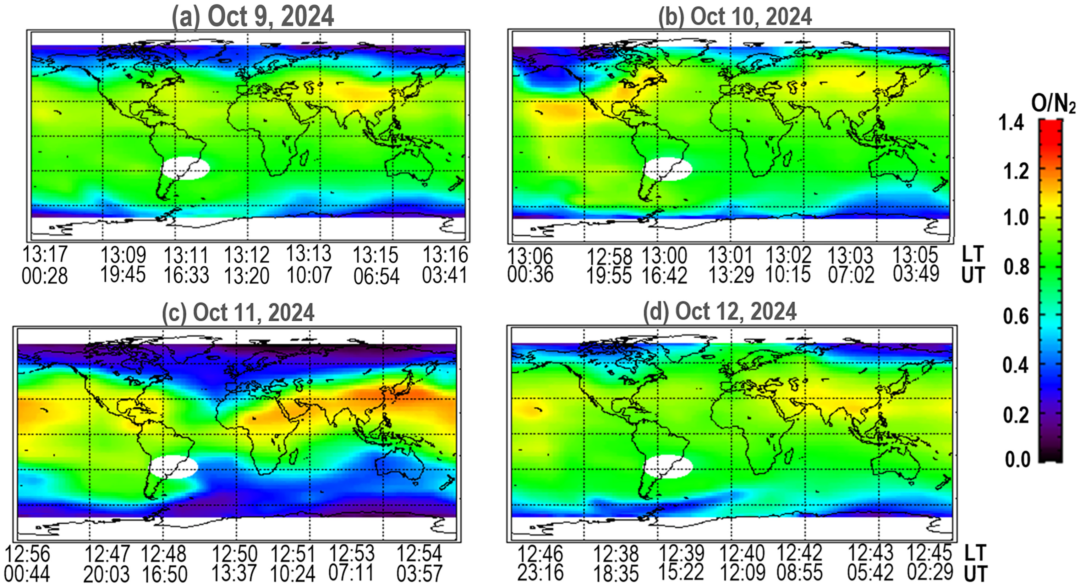
LSTID excitation was clearly observed during the main phase of the October 2024 storm (Figure 12, Figure 13, Figure 14, Figure 15, Figure 16 and Figure 17), closely linked to the storm-time thermospheric disturbances and compositional changes. The observed irregularities in Swarm Ne coincide with [O/N₂] ratio reduction (Figure 9), which enhances ion recombination and plasma loss [34]. These compositional shifts, driven by particle precipitation and Joule heating in the polar regions, modify the thermospheric circulation and are often accompanied by LSTIDs. Previous studies highlighted the link between auroral activity and LSTID generation. Borries et al. (2010) [24] found a clear correlation between AE index peaks and LSTID amplitudes, while Paul et al. (2025) [5] reported intense spatial and temporal variations in the ionosphere were driven by MIT displacement during the storms, coupled with LSTID signatures. LSTIDs, generated at high latitudes, propagated equatorward during the initial and main phases of the storm. Zhang et al. (2022) [25] and Oikonomou et al. (2022) [7] attributed LSTID formation to the intense storm-time electric field and expanded high-latitude convection field. These fields, combined with enhanced thermospheric westward wind and ion-neutral coupling, trigger ionospheric instabilities with significant growth rates. As the wind decouples from high-coupling regions, it supports the propagation of LSTIDs across middle and low latitudes. PPEFs, which rapidly map from the magnetosphere to the low-latitude ionosphere during strong southward IMF conditions, also play a crucial role. Their zonal and meridional components influence vertical and zonal plasma drift, affecting EIA and EPB formation [35]. Subsequent shielding and overshielding responses can alter or reverse these effects at mid- and low latitudes. In addition to the direct electric field effect, disturbance dynamo processes driven by storm-time neutral wind introduce the anti-Sq current systems. These include westward and poleward electric fields during the day and the eastward field at night, especially at midlatitudes [30]. Collectively, these electrodynamic and thermospheric interactions create favourable conditions for LSTID excitation and amplification during intense geomagnetic storms.

The ROTI maps over the Southeast Asian equatorial ionosphere reveal clear signatures of storm-induced EPBs during the geomagnetic storm of 10–11 October 2024. During the storm’s initial phase (15:00–17:00 UT), corresponding to local nighttime, intense ionospheric irregularities (>1 TECU/min) appeared in the Southern Hemisphere around 15:15 UT, peaked near 15:40 UT, and dissipated by 16:45 UT, with a noticeable southwestward movement. These EPBs are consistent with previous studies [26,36] showing that super EPBs can form during geomagnetic storms due to the combined effects of PRE and PPEFs, leading to rapid vertical rise and latitudinal expansion. Similar post-sunset EPB activity was also reported by Abadi et al. (2025) [26] over Southern Australia during the 2024 Mother’s Day storm. In the recovery phase, weaker perturbations (~0.4 TECU/min) were observed near the equator around 01:50 UT and 03:05–03:25 UT, likely driven by DDEFs, which are known to suppress or weakly trigger EPBs during post-midnight hours.

6. Conclusions

The present study analyzed the global ionospheric response of the geomagnetic storm recorded on 10–11 October, with a minimum SYM–H index of −346 nT. Observations revealed a substantial dayside uplift of the ionospheric F-region, evident in increased hmF2 across both Hemispheres, while foF2 remained relatively stable except for localized enhancements during the storm’s early phase. On the nightside, particularly in the Southern Hemisphere, a significant reduction in foF2 was accompanied by persistent uplift, indicating intensified recombination due to thermospheric composition changes. These responses were modulated by strong equatorward neutral winds and enhanced PPEFs driven by sustained southward IMF-Bz, which induced a large dawn-to-dusk electric field. These fields generated intensified E×B drifts exceeding 100 m/s in some regions, lifting F-region plasma to higher altitudes and latitudes, thereby enhancing plasma redistribution and contributing to the equatorial super-fountain effect. In situ measurements from Swarm and vertical drift data from Digisondes confirmed these dynamics and revealed a poleward expansion of the EIA with pronounced Hemispheric asymmetries, linked to differential particle precipitation, Joule heating, and variations in Hall conductivity. Additionally, LSTID activity was detected during all phases of the storm, propagating equatorward under the combined influence of storm-time electric fields (PPEFs and DDEFs), enhanced westward winds, and ion-neutral coupling. These drivers, intensified by high-latitude Joule heating and particle precipitation, altered thermospheric circulation and composition, creating favourable conditions for the generation, amplification, and equatorward extension of LSTIDs. The study also identified storm-induced EPBs over Southeast Asia during the main phase, likely triggered by enhanced PPEFs and PRE, followed by suppression during the recovery phase—consistent with super EPB dynamics observed in previous geomagnetic storms.

References

1. Aarons, J. Global positioning system phase fluctuations at auroral latitudes. J. Geophys. Res. 1997, 102, 17219–17231. [Google Scholar] [CrossRef]
2. Aarons, J.; Lin, B. Development of high latitude phase fluctuations during the January 10, April 10–11, and May 15, 1997 magnetic storms. J. Atmos. Sol.-Terr. Phys. 1999, 61, 309–327. [Google Scholar] [CrossRef]
3. Sori, T.; Shinbori, A.; Otsuka, Y.; Tsugawa, T.; Nishioka, M.; Yoshikawa, A. Generation mechanisms of plasma density irregularity in the equatorial ionosphere during a geomagnetic storm on 21–22 December 2014. J. Geophys. Res. Space Phys. 2022, 127, e2021JA030240. [Google Scholar] [CrossRef]
4. Paul, K.S.; Haralambous, H.; Oikonomou, C. Ionospheric response of the March 2023 geomagnetic storm over European latitudes. Adv. Space Res. 2024, 73, 6029–6040. [Google Scholar] [CrossRef]
5. Paul, K.S.; Haralambous, H.; Moses, M.; Oikonomou, C.; Potirakis, S.M.; Bergeot, N.; Chevalier, J.M. Investigation of the Ionospheric Response on Mother’s Day 2024 Geomagnetic Superstorm over the European Sector. Atmosphere 2025, 16, 180. [Google Scholar] [CrossRef]
6. Paul, K.S.; Moses, M.; Haralambous, H.; Oikonomou, C. Effects of the Mother’s Day Superstorm (10–11 May 2024) over the Global Ionosphere. Remote Sens. 2025, 17, 859. [Google Scholar] [CrossRef]
7. Oikonomou, C.; Haralambous, H.; Paul, A.; Ray, S.; Alfonsi, L.; Cesaroni, C.; Sur, D. Investigation of the negative ionospheric response of the 8 September 2017 geomagnetic storm over the European sector. Adv. Space Res. 2022, 70, 1104–1120. [Google Scholar] [CrossRef]
8. Abdu, M.A. Equatorial spread F/plasma bubble irregularities under storm time disturbance electric fields. J. Atmos. Sol.-Terr. Phys. 2012, 75–76, 44–56. [Google Scholar] [CrossRef]
9. Li, G.; Ning, B.; Wang, C.; Abdu, M.A.; Otsuka, Y.; Yamamoto, M.; Wu, J.; Chen, J. Storm-enhanced development of postsunset equatorial plasma bubbles around the meridian 120°E/60°W on 7–8 September 2017. J. Geophys. Res. Space Phys. 2018, 123, 7985–7998. [Google Scholar] [CrossRef]
10. Chu, X.; McPherron, R.L.; Hsu, T.-S.; Angelopoulos, V.; Pu, Z.; Yao, Z.; Zhang, H.; Connors, M. Magnetic mapping effects of substorm currents leading to auroral poleward expansion and equatorward retreat. J. Geophys. Res. Space Phys. 2015, 120, 253–265. [Google Scholar] [CrossRef]
11. Amadi, B.C.; Qian, L.; de Paula, E.R.; McInerney, J.M.; Kherani, E.A.; Santos, A.M.; Sanchez, S.A. Intensification and weakening of equatorial plasma bubble development observed by GOLD during different phases of a geomagnetic storm. J. Geophys. Res. Space Phys. 2023, 128, e2022JA031262. [Google Scholar] [CrossRef]
12. Foster, J.C.; Erickson, P.J.; Nishimura, Y.; Zhang, S.R.; Bush, D.C.; Coster, A.J.; Meade, P.E.; Franco-Diaz, E. Imaging the May 2024 extreme aurora with ionospheric total electron content. Geophys. Res. Lett. 2024, 51, e2024GL111981. [Google Scholar] [CrossRef]
13. Karan, D.K.; Martinis, C.R.; Daniell, R.E.; Eastes, R.W.; Wang, W.; McClintock, W.E.; Michell, R.G.; England, S. GOLD observations of the merging of the Southern Crest of the equatorial ionization anomaly and aurora during the 10 and 11 May 2024 Mother’s Day super geomagnetic storm. Geophys. Res. Lett. 2024, 51, e2024GL110632. [Google Scholar] [CrossRef]
14. Spogli, L.; Alberti, T.; Bagiacchi, P.; Cesaroni, C.; Coco, I.; Di Mauro, D.; Ippolito, A.; Marcocci, C.; Pezzopane, M.; Pica, E.; et al. The effects of the May 2024 Mother’s Day superstorm over the Mediterranean sector: From data to public communication. Ann. Geophys. 2024, 67, PA218. [Google Scholar] [CrossRef]
15. Themens, D.R.; Elvidge, S.; McCaffrey, A.; Jayachandran, P.; Coster, A.; Varney, R.H.; Galkin, I.; Goodwin, L.V.; Watson, C.; Maguire, S.; et al. The high latitude ionospheric response to the major May 2024 geomagnetic storm: A synoptic view. Geophys. Res. Lett. 2024, 51, e2024GL111677. [Google Scholar] [CrossRef]
16. Bojilova, R.; Mukhtarov, P.; Pancheva, D. Global Ionospheric Response During Extreme Geomagnetic Storm in May 2024. Remote Sens. 2024, 16, 4046. [Google Scholar] [CrossRef]
17. Pierrard, V.; Verhulst, T.G.; Chevalier, J.M.; Bergeot, N.; Winant, A. Effects of the Geomagnetic Superstorms of 10–11 May 2024 and 7–11 October 2024 on the Ionosphere and Plasmasphere. Atmosphere 2025, 16, 299. [Google Scholar] [CrossRef]
18. da Silva Picanço, G.A.; Fagundes, P.R.; Moro, J.; Nogueira, P.A.B.; Muella, M.T.; Denardini, C.M.; Resende, L.C.A.; Da Silva, L.A.; Laranja, S.R. Dynamics of Polar-Equatorial Ionospheric Irregularities During the 10–13 October 2024 Superstorm. ESS Open Archive 2025. [Google Scholar] [CrossRef]
19. Friis-Christensen, E.; Lühr, H.; Knudsen, D.; Haagmans, R. Swarm—An Earth observation mission investigating geospace. Adv. Space Res. 2008, 41, 210–216. [Google Scholar] [CrossRef]
20. Otsuka, Y.; Ogawa, T.; Saito, A.; Tsugawa, T.; Fukao, S.; Miyazaki, S. A new technique for mapping of total electron content using GPS network in Japan. Earth Planets Space 2002, 54, 63–70. [Google Scholar] [CrossRef]
21. Stauning, P. The polar cap (PC) index combination, PCC: Relations to solar wind properties and global magnetic disturbances. J. Space Weather. Space Clim. 2021, 11, 19. [Google Scholar] [CrossRef]
22. Xia, X.; Hu, X.; Wang, H.; Zhang, K. Correlation Study of Auroral Currents with External Parameters During 10–12 October 2024 Superstorm. Remote Sens. 2025, 17, 394. [Google Scholar] [CrossRef]
23. Laundal, K.M.; Cnossen, I.; Mila, S.E.; Haaland, S.E.; Coxon, J.; Pedatella, N.M.; Förster, M.; Reistad, J.P. North–South asymmetries in Earth’s magnetic field. Space Sci. Rev. 2016, 206, 225–257. [Google Scholar] [CrossRef]
24. Borries, C.; Jakowski, N.; Kauristie, K.; Amm, O.; Mielich, J.; Kouba, D. On the dynamics of large-scale travelling ionospheric disturbances over Europe on 20 November 2003. J. Geophys. Res. Space Phys. 2017, 122, 1199–1211. [Google Scholar] [CrossRef]
25. Zhang, S.R.; Nishimura, Y.; Erickson, P.J.; Aa, E.; Kil, H.; Deng, Y.; Thomas, E.G.; Rideout, W.; Coster, A.J.; Kerr, R.; et al. Traveling ionospheric disturbances in the vicinity of storm-enhanced density at midlatitudes. J. Geophys. Res. Space Phys. 2022, 127, e2022JA030429. [Google Scholar] [CrossRef]
26. Abadi, P.; Muafiry, I.N.; Pratama, T.N.; Putra, A.Y.; Pramono, G.H.; Suraina; Wibowo, S.T.; Chabibi, F.F.; Ahmad, U.A. Leveraging ROTI map derived from Indonesian GNSS receiver network for advancing study of Equatorial Plasma Bubble in Southeast. East Asia. Earth Planet. Phys. 2025, 9, 101–116. [Google Scholar] [CrossRef]
27. Vasyliunas, V.M. Mathematical models of magnetospheric convection and its coupling to the ionosphere. In Particles and Fields in the Magnetosphere, Proceedings of a Symposium Organized by the Summer Advanced Study Institute, Santa Barbara, CA, USA, 4–15 August 1969; Springer: Dordrecht, The Netherlands, 1969; pp. 60–71. Available online: https://link.springer.com/chapter/10.1007/978-94-010-3284-1_6 (accessed on 30 April 2025).
28. Fuller-Rowell, T.J.; Codrescu, M.V.; Moffett, R.J.; Quegan, S. Response of the thermosphere and ionosphere to geomagnetic storms. J. Geophys. Res. Space Phys. 1994, 99, 3893–3914. [Google Scholar] [CrossRef]
29. Tsurutani, B.T.; Verkhoglyadova, O.P.; Mannucci, A.J.; Saito, A.; Araki, T.; Yumoto, K.; Tsuda, T.; Abdu, M.A.; Sobral, J.H.A.; Gonzalez, W.D.; et al. Prompt penetration electric fields (PPEFs) and their ionospheric effects during the great magnetic storm of 30–31 October 2003. J. Geophys. Res. Space Phys. 2008, 113, A05311. [Google Scholar] [CrossRef]
30. Blanc, M.; Richmond, A.D. The ionospheric disturbance dynamo. J. Geophys. Res. Space Phys. 1980, 85, 1669–1686. [Google Scholar] [CrossRef]
31. Guo, X.; Zhao, B.; Yu, T.; Hao, H.; Sun, W.; Wang, G.; He, M.; Mao, T.; Li, G.; Ren, Z. East–west difference in the ionospheric response during the recovery phase of May 2024 super geomagnetic storm over the East Asian. J. Geophys. Res. Space Phys. 2024, 129, e2024JA033170. [Google Scholar] [CrossRef]
32. Xu, J.; Wang, W.; Gao, H. The longitudinal variation of the daily mean thermospheric mass density. J. Geophys. Res. Space Phys. 2013, 118, 515–523. [Google Scholar] [CrossRef]
33. Aa, E.; Zhang, D.; Ridley, A.J.; Xiao, Z.; Hao, Y. A global model: Empirical orthogonal function analysis of total electron content 1999–2009 data. J. Geophys. Res. A Space Phys. 2012, 117, 3328. [Google Scholar] [CrossRef]
34. Prölss, G.W. Ionospheric F-region storms. In Handbook of Atmospheric Electrodynamics; CRC press: Boca Raton, FL, USA, 1995; pp. 195–248. Available online: https://www.taylorfrancis.com/chapters/edit/10.1201/9780203713297-8/ionospheric-region-storms-gerd-pr%C3%B6lss (accessed on 30 April 2025).
35. Huang, C.S. Long-lasting penetration electric fields during geomagnetic storms: Observations and mechanisms. J. Geophys. Res. Space Phys. 2019, 124, 9640–9664. [Google Scholar] [CrossRef]
36. Sun, W.J.; Li, G.Z.; Zhang, S.R.; Hu, L.H.; Dai, G.F.; Zhao, B.Q.; Otsuka, Y.; Zhao, X.K.; Xie, H.Y.; Perwitasari, S. Regional ionospheric super bubble induced by significant upward plasma drift during the 1 December 2023 geomagnetic storm. J. Geophys. Res. Space Phys. 2024, 129, e2024JA032430. [Google Scholar] [CrossRef]
Figure 1. Solar flare effects recorded on 9 October: (a) the locations of AR3848, (b) AR3842 (red circle) over the solar disc, and (c) solar flares recorded on 9 October.
Remotesensing 17 02329 g001
Figure 2. Geomagnetic conditions during the October storm event depicted in (a) total magnitude B of IMF, (b) Bz component of IMF, (c) solar wind speed, (d) solar wind pressure, (e) interplanetary electric field (IEF) Ey, (f) SYM-H and Kp index and (g) Polar Cap (PCN) Index. The orange vertical lines represent the SSC, the grey vertical line denotes the time of the SYM-H index minima during the storm, the purple vertical line represents when SYM–H < −100 nT, and the brown vertical line represents the end of the recovery phase of the ionosphere.
Remotesensing 17 02329 g002
Figure 3. (ah) Variation in foF2 (MHz) from COSMIC—2 RO during 9–11 October from (a) 00:00–03:00 UT, (b) 03:00–06:00 UT, (c) 06:00–09:00 UT, (d) 09:00–12:00 UT, (e) 12:00–15:00 UT, (f) 15:00–18:00 UT, (g) 18:00–21:00 UT, and (h) 21:00–24:00 UT. The yellow highlighted section represents the storm period (initial phase of the storm to SYM–H < −100 nT during the recovery phase). The red rectangles in the subfigures represent the absence of foF2 values during the storm period.
Remotesensing 17 02329 g003
Figure 4. (ah) Variation in hmF2 (km) from COSMIC—2 RO during 9–11 October from (a) 00:00–03:00 UT, (b) 03:00–06:00 UT, (c) 06:00–09:00 UT, (d) 09:00–12:00 UT, (e) 12:00–15:00 UT, (f) 15:00–18:00 UT, (g) 18:00–21:00 UT, and (h) 21:00–24:00 UT. The yellow highlighted section represents the storm period (initial phase of the storm to SYM–H < −100 nT during the recovery phase). The red rectangles in the subfigures represent the absence of hmF2 values during the storm period.
Remotesensing 17 02329 g004
Figure 5. (ah) Electron density profiles of COSMIC—2 RO on 11 October from 00:00–03:00 UT over the region “A” marked in Figure 4a.
Remotesensing 17 02329 g005
Figure 6. (ah) Electron density profiles of COSMIC—2 RO on 11 October from 03:00–06:00 UT over the region “B” marked in Figure 4b.
Remotesensing 17 02329 g006
Figure 7. (ah) Electron density profiles of COSMIC—2 RO on 11 October from 09:00–12:00 UT over the region “C” marked in Figure 4d.
Remotesensing 17 02329 g007
Figure 8. (ac) Drift velocity components: (a) vertical drift, (b) north–south component of horizontal drift, and (c) east–west component of horizontal drift over three stations from 10 October to 12 October. The orange vertical lines represent the SSC, the grey vertical line denotes the time of the SYM-H index minimum during the storm, the pink line represents when SYM–H < −100 nT during the recovery period, and the brown vertical line represents the end of the recovery phase of the ionosphere.
Remotesensing 17 02329 g008
Figure 9. (ad) Global variation in [O/N2] ratio on (a) 9 October, (b) 10 October, (c) 11 October, and (d) 12 October.
Remotesensing 17 02329 g009
Figure 10. (at) Three-hour global tracks of Swarm Ne (Swarm A represented by brown tracks and Swarm B represented by blue tracks). The leftmost column represents the Swarm tracks from 15:00 UT on 5 October to 06:00 UT on 6 October, a geomagnetically quiet period for reference. The second column depicts the storm-time Swarm tracks from 15:00 UT on 10 October to 06:00 UT on 11 October. The third and fourth columns represent the madrigal global TEC maps during the geomagnetically quiet and disturbed periods.
Remotesensing 17 02329 g010
Figure 11. (at) Three-hour global tracks of Swarm Ne (Swarm A represented by brown tracks and Swarm B represented by blue tracks). The leftmost column represents the Swarm tracks from 06:00 UT to 21:00 UT on 6 October, a geomagnetically quiet period for reference. The second column depicts the storm-time Swarm tracks from 06:00 UT to 21:00 UT on 11 October. The third and fourth columns represent the madrigal global TEC maps during the geomagnetically quiet and disturbed periods.
Remotesensing 17 02329 g011
Figure 12. (ad) LSTIDs detected in the global dTEC map over the Northern Hemisphere on 10 October during (a) 15:20UT, (b) 15:30UT, (c) 15:40UT, and (d) 15:50UT.
Remotesensing 17 02329 g012
Figure 13. (ad) LSTIDs detected in the global dTEC map over the Northern Hemisphere on 10 October during (a) 17:00 UT, (b) 17:10UT, (c) 17:20UT, and (d) 17:40UT.
Remotesensing 17 02329 g013
Figure 14. (ad) LSTIDs detected in the global dTEC map over the Northern Hemisphere on 10 October during (a) 19:10UT, (b) 19:20UT, (c) 19:40UT, and (d) 19:50UT.
Remotesensing 17 02329 g014
Figure 15. (ad) LSTIDs detected in the global dTEC map over the Northern Hemisphere on 10 October (a) 20:50UT, (b) 21:10UT, (c) 21:30UT, and (d) 21:40UT.
Remotesensing 17 02329 g015
Figure 16. (ah) LSTIDs detected in the global dTEC map over the Northern Hemisphere on 10 October during (a) 22:10UT, (b) 22:30UT, (c) 22:50UT, (d) 23:00 UT, (e) 23:10UT, (f) 23:20UT, (g) 23:30UT, and (h) 23:40UT.
Remotesensing 17 02329 g016
Figure 17. (ah) LSTIDs detected in the global dTEC map over the Northern Hemisphere on 10 October during (a) 01:20UT, (b) 01:30UT, (c) 01:40UT, (d) 01:50UT, (e) 02:00 UT, (f) 02:10UT, (g) 02:20UT, and (h) 02:30UT.
Remotesensing 17 02329 g017
Figure 18. (ac) The storm time ROTI–map over the Southeast Asian region (a) from 15:15 UT to 17:00 UT of 10 October, (b) 01:50 UT to 02:00 UT, and (c) 03:05 UT to 03:25 UT of 11 October.
Remotesensing 17 02329 g018
Disclaimer/Publisher’s Note: The statements, opinions and data contained in all publications are solely those of the individual author(s) and contributor(s) and not of MDPI and/or the editor(s). MDPI and/or the editor(s) disclaim responsibility for any injury to people or property resulting from any ideas, methods, instructions or products referred to in the content.