Abstract
Multi-source remote sensing spatiotemporal fusion aims to enhance the temporal continuity of high-spatial, low-temporal-resolution images. In recent years, deep learning-based spatiotemporal fusion methods have achieved significant progress in this field. However, existing methods face three major challenges. First, large differences in spatial resolution among heterogeneous remote sensing images hinder the reconstruction of high-quality texture details. Second, most current deep learning-based methods prioritize spatial information while overlooking spectral information. Third, these methods often depend on complex network architectures, resulting in high computational costs. To address the aforementioned challenges, this article proposes a Sparse Fast Transformer fusion method based on Generative Adversarial Network (SFT-GAN). First, the method introduces a multi-scale feature extraction and fusion architecture to capture temporal variation features and spatial detail features across multiple scales. A channel attention mechanism is subsequently designed to integrate these heterogeneous features adaptively. Secondly, two information compensation modules are introduced: detail compensation module, which enhances high-frequency information to improve the fidelity of spatial details; spectral compensation module, which improves spectral fidelity by leveraging the intrinsic spectral correlation of the image. In addition, the proposed sparse fast transformer significantly reduces both the computational and memory complexity of the method. Experimental results on four publicly available benchmark datasets showed that the proposed SFT-GAN achieved the best performance compared with state-of-the-art methods in fusion accuracy while reducing computational cost by approximately 70%. Additional classification experiments further validated the practical effectiveness of SFT-GAN. Overall, this approach presents a new paradigm for balancing accuracy and efficiency in spatiotemporal fusion.
1. Introduction
Remote sensing has been extensively used in a wide range of Earth observation tasks, including continuous crop growth monitoring for agricultural assessment [1,2,3], analysis of the water environment [4,5], and long-term ecosystem evaluations such as forest cover change [6,7,8] as well as desertification monitoring [9,10,11]. The dynamic monitoring of the ground surface requires remote sensing data with high spatial and temporal resolutions. Current mainstream optical remote sensing data can be categorized into hyperspectral, multispectral, and panchromatic images. Hyperspectral images typically consist of hundreds of contiguous narrow spectral bands (e.g., 100–200 bands within the 400–2500 nm range), providing a high spectral resolution but relatively low spatial and temporal resolutions. Panchromatic images consist of only one broad spectral band and produce grayscale imagery with the highest spatial resolution, but they lack rich spectral information. Multispectral images typically include 4–20 relatively broad bands, striking a balance with moderate spatial and temporal resolutions and are widely used in various applications. However, existing multispectral satellite systems face a fundamental trade-off: relatively high-spatial-resolution satellites (e.g., Landsat) are limited by a narrow width and long revisit period, resulting in inadequate temporal continuity; and high-frequency observing systems (e.g., MODIS) are constrained by a low spatial resolution, which makes it difficult to capture the detailed features of the ground surface. To address this limitation, multi-source remote sensing spatiotemporal fusion techniques have emerged as a promising solution. These techniques fuse multispectral imagery from different sources. The main concept of spatiotemporal fusion is to generate high-quality images with both fine spatial and temporal resolutions by integrating complementary information from multiple remote sensing sources [12].
Spatiotemporal fusion methods generate fused images by extracting spatial details and capturing temporal variations. The fundamental principle is to establish a mapping between temporal changes and spatial structures through the synergistic integration of multispectral high-spatial–low-temporal-resolution images (fine-resolution images) and multispectral low-spatial–high-temporal-resolution images (coarse-resolution images). Existing spatiotemporal fusion approaches are broadly categorized into two groups: traditional model-driven methods and data-driven deep learning methods [13]. Traditional model-driven approaches are further divided into three main types: weight function-based, unmixing-based, and sparse representation-based methods. Weight function-based methods model coarse-to-fine image relationships using spatiotemporal neighborhood similarity and weighting functions [14]. For example, The Spatial and Temporal Adaptive Reflectance Fusion Model (STARFM) [15] assumes coarse pixel spectral purity and transfers reflectance changes via weighting to predict the target fine image from a prior one. While flexible and physically interpretable, these methods often fail in areas of abrupt land surface change. Unmixing-based methods [16,17] apply linear spectral mixture theory, decomposing coarse pixels into endmembers (pure land cover spectra) and their abundances (fractional cover). They reconstruct fused images by integrating fine image spatiotemporal information. The Flexible Spatiotemporal Data Fusion Algorithm (FSDAF) [18] combines weight function and unmixing concepts: it estimates homogeneous region spectral variations, interpolates spatial changes, and fuses spectral and spatial features to generate fine images. Unmixing methods offer fine pixel decomposition and handle local changes well but struggle with subtle land cover transitions. Sparse representation-based methods [19] decompose images into sparse dynamic and low-rank static components. Within a sparse coding framework, they jointly model coarse image temporal evolution and a fine image global structure, suppressing noise while enhancing spatiotemporal consistency and preserving fine details. The Error-Bound-Regularized Sparse Coding Dictionary Learning (EBSCDL) model [20] employs error-bound regularization to constrain dictionary perturbations and block-sparse constraints to better model local structural correlations. However, these methods’ strong reliance on local sparsity limits their ability to model cross-scale dependencies and complex nonlinear dynamics, consequently restricting their preservation of global consistency and representation of sudden changes.
Compared with traditional model-driven methods, deep learning-based methods can capture the complex spatiotemporal relationships implicit in large-scale remote sensing data. As a result, deep learning has been extensively applied in spatiotemporal fusion tasks in recent years [21]. Generative Adversarial Network (GAN) [22], as a revolutionary generative model, has been widely used in image generation, super-resolution, and other fields [23]. Consequently, GAN has also been introduced into remote sensing spatiotemporal fusion tasks [24,25,26]. The GAN-STFM method [27] breaks the temporal constraints on reference image selection, significantly improving the flexibility of the fusion process. However, this increased flexibility may compromise the accuracy of the fused images. The PSTAF-GAN method [28] designs a flexible multi-scale feature extraction framework to capture hierarchical features and adopts a progressive fusion strategy to enhance fusion accuracy. The MLFF-GAN method [29], based on the U-Net architecture, adopts multi-level feature fusion to improve fusion accuracy in regions undergoing change. The HPLTS-GAN method [30] is designed to enhance model performance in temporally insensitive tasks by minimizing reliance on temporal information while preserving prediction accuracy. This approach effectively improves the spatiotemporal consistency of the fused images and substantially enhances the model’s overall performance.
The convolutional neural network (CNN), known for its powerful feature extraction capabilities, has become one of the most prominent approaches in multi-source remote sensing image spatiotemporal fusion [31,32,33,34]. The Enhanced Deep Convolutional Spatiotemporal Fusion Network (EDCSTFN) [35] uses multi-receptive-field convolutional layers to extract multi-scale spatial features. Deeper layers capture abstract semantic information, while shallower layers preserve high-frequency details, improving the modeling of complex land cover. However, despite its strong spatiotemporal performance, it struggles to capture subtle long-term temporal variations. The MLKNet method [36] introduces a multi-level knowledge modeling mechanism to fully leverage the complementary nature of hierarchical features, such as shallow structural information and deep semantic representations, thereby enhancing the network’s capability to model complex scenes. The CIG-STF method [37] effectively integrates change detection with spatiotemporal fusion, substantially improving fusion accuracy for abrupt land cover changes (such as floods and landslides) in fused images, thereby enhancing the model’s practicality.
CNN is effective at extracting local image features but struggles to model long-range dependencies. In contrast, the transformer leverages self-attention to model global dependencies, making it well-suited for tasks involving long-range context understanding and cross-modal learning. These advantages have contributed to the widespread adoption of the Vision Transformer (ViT) [38] in computer vision. ViT employs self-attention to capture global relationships between image patches, enabling robust global feature representation, especially when trained on large-scale datasets. Several ViT-based approaches have been proposed for spatiotemporal fusion in remote sensing [39,40,41]. For example, STINet [42] fuses multi-scale spatiotemporal features to capture variations across land cover types, but it may introduce local texture distortions. STM-STFNet [43] integrates Swin Transformer’s global context modeling with multi-dimensional attention to jointly predict images in both spatial and temporal domains. This design improves accuracy under complex surface changes, such as land cover transitions. SwinSTFM [44] combines pixel-level attention with spectral mixture theory to enhance fusion performance. However, similar to other transformer-based approaches, it suffers from a high computational complexity.
In summary, while many deep learning-based spatiotemporal fusion methods have achieved promising performance, several limitations remain:
- In spatiotemporal fusion tasks, the significant resolution gap between coarse- and fine-resolution images poses a major challenge for reconstructing high-quality texture details.
- Existing deep learning-based spatiotemporal fusion methods often emphasize spatial details while neglecting spectral information, resulting in fused images with high spatial fidelity but significant spectral distortion.
- Most existing end-to-end deep learning-based spatiotemporal fusion methods rely on relatively complex neural network architectures, which often lead to a high computational complexity. The massive data volumes of remote sensing images further intensify this computational burden.
Although existing deep learning-based methods have achieved impressive results, no comprehensive solution has been proposed to address all three issues simultaneously. To address the aforementioned limitations, this article proposes a deep learning-based model, Sparse Fast Transformer fusion method based on Generative Adversarial Network (SFT-GAN). Compared to existing deep learning-based multi-source remote sensing spatiotemporal fusion methods, the proposed SFT-GAN offers the following contributions:
- To concentrate on the first limitation, SFT-GAN adopts a multi-level pyramid architecture and designs a flexible channel attention fusion mechanism to adaptively fuse spatial detail features and temporal variation features, enhancing informative channels while suppressing irrelevant noise. In addition, a Detail Compensation Module (DCM) is introduced to fully leverage spatial prior information from the reference image. The DCM applies the Butterworth filter to decompose the image into high- and low-frequency components at multiple scales, enhancing the high-frequency details to improve texture representation.
- To address the second limitation, a Spectrum Compensation Module (SCM) is designed to leverage spectral prior information from reference images. Specifically, SCM analyzes inter-band correlations in coarse-resolution images to extract intrinsic spectral patterns, which are used to guide the reconstruction of fine-resolution images, thereby enhancing the spectral fidelity of the fused image.
- To focus on the third limitation, this article proposes the Sparse Transformer Module, which optimizes the transformer using a KL divergence-based sparsity strategy, significantly reducing the model’s computational complexity and memory consumption. Under the same training conditions, the proposed method can process larger-scale datasets, thereby improving overall efficiency and practical applicability.
The remaining contents are organized as follows. Section 2 presents the overall architecture of the proposed SFT-GAN model. Section 3 validates the effectiveness of the proposed method through both comparative and ablation experiments. Section 4 discusses the proposed method’s performance and advantages and outlines potential directions for future research. Section 5 concludes the article and outlines potential directions for future work. Additional, the code is released at https://github.com/MaZhaoX/SFT-GAN (accessed on 2 July 2025).
2. Methodology
SFT-GAN is a deep learning-based spatiotemporal fusion model based on Generative Adversarial Network (GAN), integrating multiple modules to accurately capture spatiotemporal features and optimize fusion quality. The overall framework is illustrated in Figure 1, consisting of two main components: the generator and the discriminator. The generator (Section 2.1) comprises four key modules that work together to progressively enhance the image quality and detail representation. The Sparse Transformer Module (Section 2.1.1) constructs a multi-scale feature extraction mechanism, extracting both temporal variation features and spatial detail features. One Sparse Transformer Module captures temporal variation features between the coarse-resolution images at time and at time , while the other focuses on the fine-resolution image at time , extracting its spatial detail features. The Feature Reconstruction Module (Section 2.1.2) reconstructs a preliminary fused image using the extracted spatiotemporal features. The Detail Compensation Module (Section 2.1.3) enhances texture details in the preliminary fused image to improve visual fidelity. The Spectrum Compensation Module (Section 2.1.4) extracts the inter-band correlations from the coarse-resolution image at time and performs spectral optimization on the detail-enhanced fused image, ensuring consistency in spectral characteristics. The discriminator (Section 2.2) distinguishes between real fine-resolution images and fused images generated by the generator. The generator and discriminator are trained adversarially to improve the quality of the fused image.
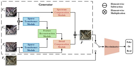
Figure 1.
Architecture of the spatiotemporal fusion GAN network. denotes the coarse-resolution image at time ; denotes the fine-resolution image at time . denotes the fine-resolution image at time , which also serves as the ground truth for the discriminator; represents the fused image. The discriminator selects either or as input.
2.1. Generator
The generator consists of four parts: Sparse Transformer Module, Feature Reconstruction Module, Detail Compensation Module, and Spectrum Compensation Module. Its overall structure is illustrated in Figure 2. The Sparse Transformer Module extracts both spatial detail features and temporal variation features independently. The Feature Reconstruction Module reconstructs the spatial detail features and the temporal variation features into a preliminary fusion image . The Detail Compensation Module is used to compensate for the detailed texture information of the preliminary fusion image, and the Spectrum Compensation Module corrects spectral distortions, finally resulting in the fine-resolution fused image .
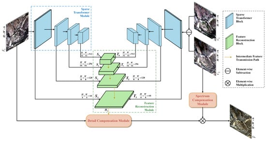
Figure 2.
Generator workflow diagram. The blue modules at the top consist of two Sparse Transformer Modules. The left module is designed to extract fine spatial features, while the right module captures temporal variation features. The green module at the bottom is designated as the Feature Reconstruction Module, where the Detail Compensation Module compensates for detailed information and the Spectrum Compensation Module compensates for spectral information. denotes the fine-resolution image at time , denotes the coarse-resolution image at time , denotes the fine-resolution image at time , and represents the fused image.
2.1.1. Sparse Transformer Module
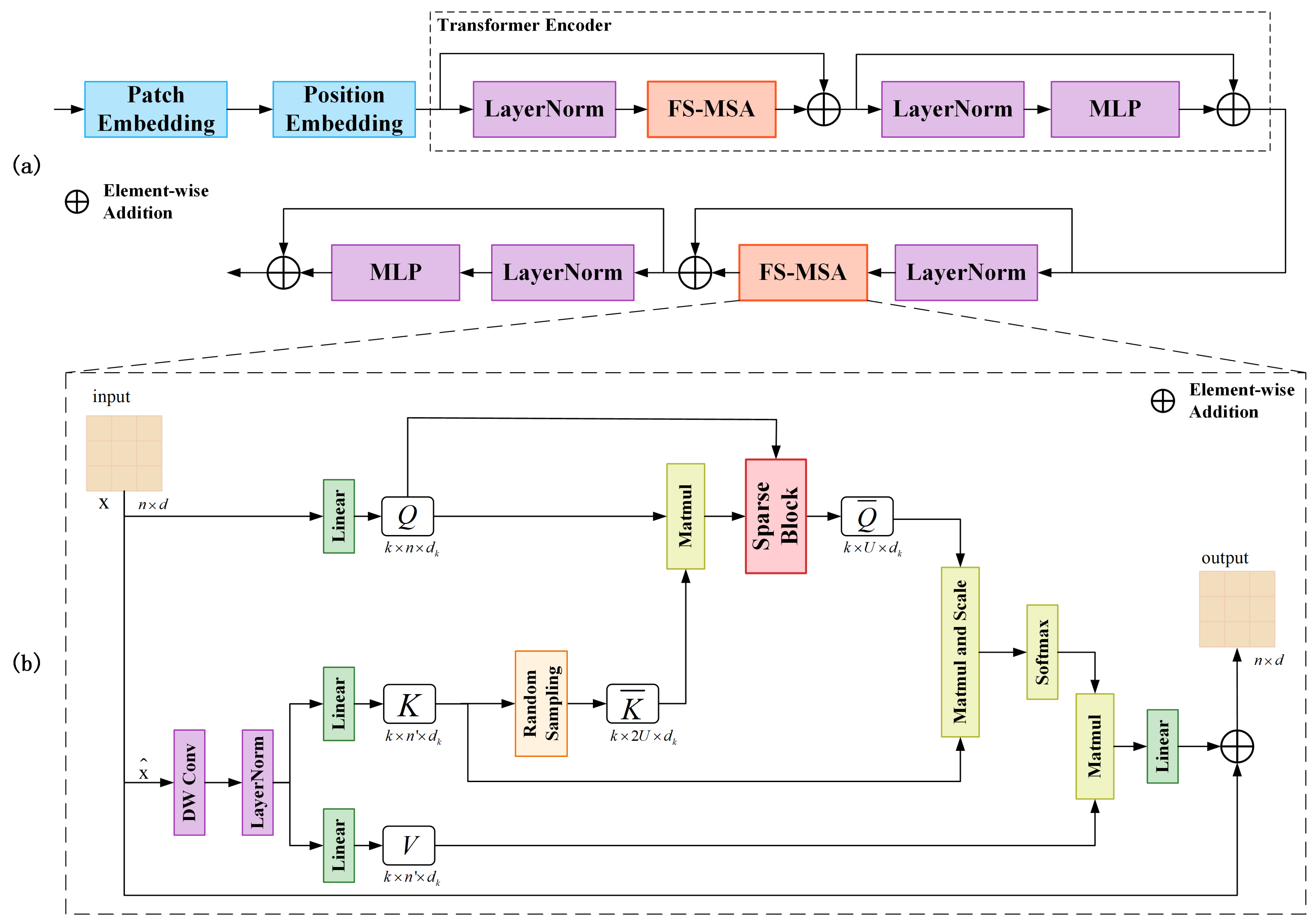
The Vision Transformer (ViT) has been widely adopted in computer vision. However, it continues to face challenges due to its high computational and memory requirements. Remote sensing images typically contains much larger data volumes than natural images due to their high spatial resolution, multispectral or hyperspectral bands, high radiometric resolution, and extensive spatial coverage. As a result, applying ViT to remote sensing images leads to even greater computational complexity. To mitigate this issue, we propose a content-aware Sparse Transformer Block (STB), as shown in Figure 3. Recent studies have explored incorporating sparse attention into transformers to reduce computational complexity [45,46,47]. In multi-head self-attention, sparsity implies that each position attends to only a subset of key positions rather than all positions in the sequence.
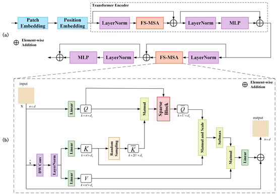
Figure 3.
The network architecture diagram of the Sparse Transformer Block (STB). (a) STB workflow diagram. The STB consists of a Patch Embedding, a Position Embedding, and two Transformer Encoders. (b) Architecture of FS-MSA.
The Sparse Transformer Module comprises four STBs, each of which contains two consecutive transformer encoders. Compared to the multi-head self-attention (MSA) in ViT, the fast sparse multi-head self-attention (FS-MSA) in STB significantly reduces both computational complexity and space complexity. The structure of FS-MSA is illustrated in Figure 3. The two-dimensional input token is first reshaped into a three-dimensional form , which is then processed by deep convolutional and LayerNorm layers. The feature map size is proportionally reduced, with the reduction ratio adaptively determined according to the input size. This process effectively performs a downsampling on the input image, reducing the number of image patches when the image is converted into a sequence. The results from the deep convolutional layers and LayerNorm are then reshaped back into a two-dimensional form. key K and value V are obtained via projection, while the query Q is directly projected from the original input x. The Sparse Block serves as the core component of FS-MSA, responsible for sparsifying the query Q. A detailed analysis of the Sparse Block is presented below.
The attention mechanism can be viewed as a querying process, where Q and K are used to compute similarity scores to obtain attention weights, which are then used to perform a weighted sum over V. In other words, it represents a form of soft querying mechanism [48]. The Softmax normalized attention weights are non-negative and sum to 1, thus having the characteristics of a probability distribution. Ideally, each query vector q contributes equally to the attention features, implying a uniform distribution. If the attention weights associated with a query vector q deviate from the uniform distribution, it indicates that q contributes more significantly to the attention features. Conversely, if the attention weights are approximately uniform, the contribution of q is close to average, suggesting that it has a relatively average influence on the attention representation. In this article, the Kullback–Leibler () divergence is used to quantify the difference between the probability distribution of a query vector q and the uniform distribution, as shown in Equation (1), which is further simplified to yield Equation (2).
where denotes the probability distribution of the i-th query q over the j-th key k, while represents the uniform distribution of the i-th query q over the j-th key k, where L is the length of the sequence after transforming the image into patches. Since attention weights are typically discrete, kernel smoothing is applied to obtain a smoother probability distribution suitable for KL divergence computation, so that is the result of kernel smoothing, and we substitute this into Equation (2) to obtain the following:
where is the exponential kernel , and we substitute it into Equation (3) to obtain
Further, this article defines the sparsity dispersion measure of the i-th vector q as
where represents the sparsity dispersion measure of the ith query vector q, is the LogSumExp (LSE) operation, while denotes their arithmetic mean. A higher value of indicates that the i-th query vector q contributes more significantly to the attention features. However, computing this value still requires intensive computation. To facilitate efficient estimation, this article proposes a heuristic approximation method, as shown in Equation (6), to approximate the sparsity divergence measure of the query vector q.
To identify the query vectors q with significant contributions to the attention weights, the dot-product pairs are randomly selected to approximate the sparsity divergence . Based on the values of , the top query vectors are chosen, as they are deemed to have substantial contributions to the attention weights. These selected query vectors are grouped into and used for self-attention computation. This approach avoids computing all dot-product pairs, thereby significantly improving computational efficiency. Therefore, this approach adopts a random sampling strategy to select a subset of dot-product pairs for computing . The number of samples, denoted as , increases with the sequence length L. This ensures that even for large-scale images, a sufficient number of samples is retained, thus preventing potential accuracy loss in the final fusion caused by random sampling.
2.1.2. Feature Reconstruction Module
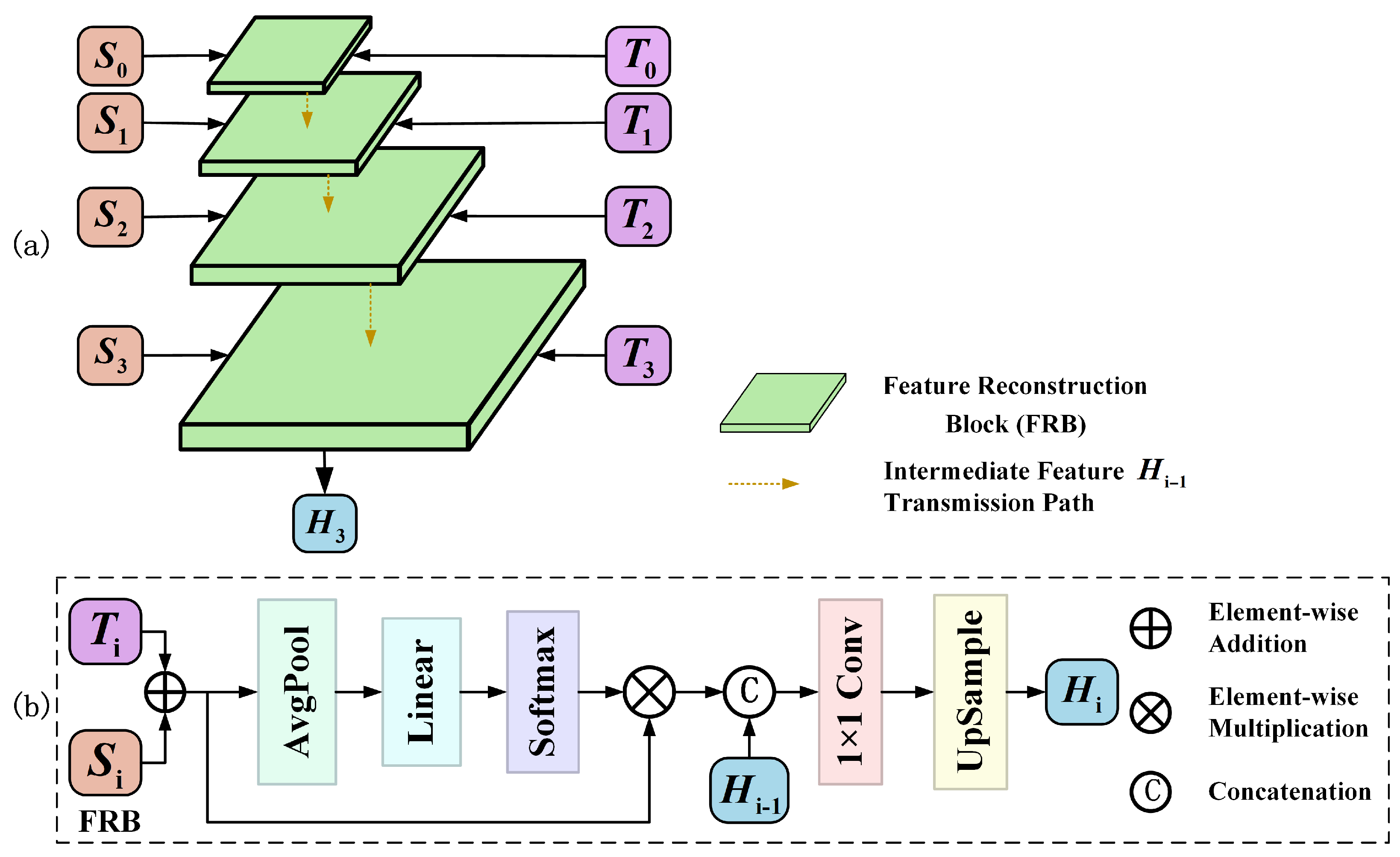
The proposed Feature Reconstruction Module (FRM) consists of four stages, each containing a Feature Reconstruction Block (FRB). The structures of the FRM and FRB are illustrated in Figure 4. Each FRB is built upon a channel attention mechanism and is designed to fuse spatial detail features and temporal variation features at the same scale. The FRB first adds the spatial detail features and temporal variation features, and the resulting feature map is passed through a channel attention module composed of Average Pooling and Linear and Softmax layers to compute channel-wise importance weights and refine the features accordingly. Then, a convolution and an upsampling operation are applied to adjust the size and number of channels of the feature maps to fit the next-level FRB. After four stages of feature fusion, the preliminary high-resolution fused image is obtained.

Figure 4.
Architecture of the Feature Reconstruction Module (FRM). (a) The FRM flowchart consists of four stages, each with a similar structure to the Feature Reconstruction Block (FRB), ultimately producing the initial fine-resolution image . (b) Architecture of FRB. Input represents the temporal variation features, represents the fine spatial features, and represents the fused features from the previous scale. Output represents the fused features at the current scale.
The FRB learns the importance weights of different channels via a channel attention mechanism, enabling it to adaptively adjust the contribution of each channel within the spatiotemporal features. Since certain channels in MODIS images are affected by striping noise, the attention mechanism suppresses these noisy channels and amplifies the contribution of information-rich ones during the fusion process, thereby reducing the adverse impact of noise from the reference images on the final fused image. The Feature Reconstruction Module adopts a channel-attention-guided adaptive fusion strategy that directs the model’s focus toward channels with high semantic consistency, thereby enhancing its sensitivity to spatial information. This approach effectively alleviates the negative effects of resolution disparities between coarse- and fine-resolution images, resulting in high-quality detail reconstruction.
2.1.3. Detail Compensation Module
To enhance the texture details of the image, we adopt a multi-scale strategy for high-frequency information enhancement. Specifically, we perform frequency domain decomposition to separate the high-frequency and low-frequency components of the image, where texture details are primarily contained in the high-frequency components. Therefore, enhancing the high-frequency components effectively compensates for texture details. First, multiple Butterworth low-pass filters with different cutoff frequencies are used to extract low-frequency components at various scales. Then, multi-scale high-frequency information is obtained by computing the difference between the input image and the corresponding low-frequency images. These high-frequency components capture texture details ranging from coarse to fine scales. Subsequently, the multi-scale high-frequency components are adaptively fused with the original image through a linear combination, resulting in a refined fused image with enhanced texture details. In the Detail Compensation Module, we use three Butterworth low-pass filters to extract low-frequency components at three different scales.
Here, , , and denote the three Butterworth low-pass filters, with cutoff frequencies of 250, 150, and 100, and corresponding filter orders of 2, 4, and 4, respectively. Subsequently, high-frequency components at different scales, denoted as , , , , and , are extracted through differencing operations, as shown in the following equation:
Here, represents the fine-resolution image at time ; represents the high-frequency spatial prior information contained in the fine-resolution image at time ; and represent the fine-scale high-frequency information of the fused image, while and represent the coarse-scale high-frequency information of the fused image.
The core components of the Detail Compensation Module lie in the adaptive strategy used during the linear fusion process. We design two adaptive weighting functions, and , where adjusts the contribution of the high-frequency spatial prior information from the reference fine-resolution image, while adjusts the weights of the remaining high-frequency components. When linearly fusing the high-frequency component with the input image, tends to amplify pixel intensity differences near image edges, potentially leading to over-enhancement and overshoot artifacts at the boundaries. To alleviate this effect in the final fused image, we introduce to suppress the positive values of while enhancing its negative values, thus mitigating overshoot artifacts. The weighting function exhibits a nonlinear stretching property, providing a continuous and smooth transition that helps reduce overshoot artifacts and discontinuities at image edges, enhancing the visual consistency of the fused image.
Here, denotes the sign function. The linear fusion of the multi-scale high-frequency components with the input image is performed as follows:
2.1.4. Spectrum Compensation Module
The Spectrum Compensation Module is based on the assumption of multisensor radiometric response consistency, which posits that different sensors yield consistent radiometric responses to the same land surface under identical temporal conditions. As a result, the spectral information in the resulting remote sensing images is expected to be consistent. This module enhances the spectral fidelity of the fused image by leveraging the inherent spectral correlation patterns present in the coarse-resolution image. Specifically, it first learns the inter-band relationships of the coarse-resolution image at time , and it subsequently transfers this learned spectral structure to the fused image , which has already undergone texture detail compensation. This process ensures that the fused image preserves more accurate and consistent spectral information. The architecture of the Spectrum Compensation Module is illustrated in Figure 5.
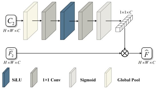
Figure 5.
Architecture of the Spectrum Compensation Module (SCM). The input is the coarse image at time , and the output is a 1 × 1 × C weight matrix representing the inter-band relationships.
The Spectrum Compensation Module leverages the spectral prior information from the coarse-resolution image at time . It first integrates spatial information through a global pooling operation, thereby capturing the global features of the entire image. The pooled features are then processed by a convolutional layer that doubles the number of channels and uses the SiLU activation function to learn complex inter-channel relationships. A subsequent convolutional layer reduces the channel dimension back to its original size, further refining the spectral weighting information. Finally, the output is normalized to the [0, 1] range using a Sigmoid activation function, resulting in the generation of spectral weights. These spectral weights represent the inter-band correlations within the coarse-resolution image at time . Under the assumption of consistent radiometric responses across sensors, the spectral bands of the fine-resolution image at time are expected to exhibit similar inter-band relationships. Accordingly, the proposed method applies the learned spectral weights to the detail-compensated fused image through element-wise multiplication, thereby adjusting its inter-band correlations. This process performs spectral information compensation and yields the final fused image .
2.2. Discriminator
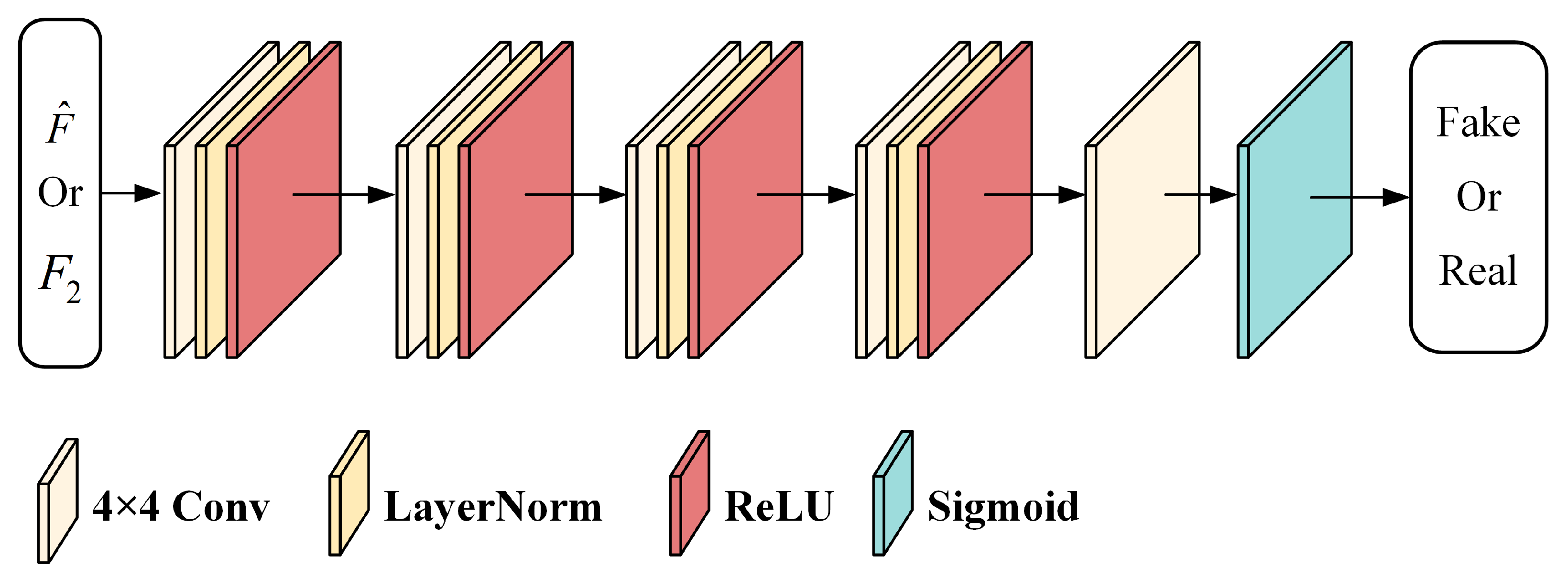
The discriminator of the SFT-GAN is a binary CNN classifier, as illustrated in Figure 6. The discriminator determines whether the input image patch is a fused image or a real image. The convolutional blocks in the discriminator consist of convolutional layers, LayerNorm layers, and ReLU activation functions. During training, when the input is the real image , a fully real matrix is expected, while a fully fake matrix is expected when the input is the fused image . The discriminator uses even-sized convolutional kernels, which helps uniformly learn features and prevents overemphasizing or neglecting specific pixels during convolution, thereby enhancing the discriminator’s ability to differentiate between generated and real samples. These advantages facilitate the training of the generator, ensuring that the distribution of the fused image closely matches that of the real image.

Figure 6.
Architecture of the Discriminator. The discriminator comprises four convolutional blocks and a convolutional layer, and it employs the Sigmoid function.
2.3. Loss Function
The loss function used in the proposed method consists of two main components: GAN loss and image loss. The GAN loss is based on the Least Squares GAN (LSGAN) [49,50], as defined in Equations (16) and (17). The image loss is composed of loss, spectral loss, and structural loss.
where a, b, and c are constants; a and b are labels for false and true data, respectively; and c denotes the value of the false data that the generator wants the discriminator to believe.
The loss is used to constrain the pixel values of the fused image and the real image to be equal at corresponding spatial locations, as defined in Equation (18). The spectral loss uses cosine similarity to ensure that the spectrum of the generated image closely matches that of the real image, as defined in Equation (19). The structural loss is based on MS-SSIM, as defined in Equation (20).
Here, denotes the real image, represents the fused image, K is the number of pixels in the image, and denotes the p-norm. In Equation (20), M represents the highest scale; , , and are the luminance, contrast, and structure measures at the j-th scale, respectively. , , and are the corresponding weight coefficients.
Finally, the overall loss is defined as follows:
3. Experiments and Results
3.1. Study Areas and Datasets
The experiments use publicly available datasets from two locations: the Lower Gwydir Catchment (LGC) and the Coleambally Irrigation Area (CIA) [51]. The study area of LGC is located in northern New South Wales (NSW) and contains 14 pairs of cloud-free Landsat-MODIS (L-M) image pairs acquired between April 2004 and April 2005. Both the Landsat and MODIS images are resampled to a size of 2720 × 3200 pixels with a spatial resolution of 25 m, and each image contains six spectral bands. A flood occurred in this area in December 2004, rendering it a dynamic site for testing temporal robustness. This enables a more effective evaluation of the method’s predictive performance under dynamic land cover conditions. The study area of CIA is located in southern NSW, consisting of 17 cloud-free L-M image pairs from 2001 to 2002, resampled to 2040 × 1720 pixels for spatiotemporal fusion. The agricultural and forest areas surrounding the CIA region exhibit considerable temporal variability despite minimal changes in land cover types. Consequently, although land cover remains relatively stable, the CIA dataset displays notable temporal variation.
As the LGC and CIA datasets primarily cover plains and farmlands, the temporal gaps between adjacent image pairs are typically a few days and phenological changes are relatively mild. To further assess the generalization and applicability of the methods, additional experiments were conducted using the AHB and Tianjin datasets [52]. The AHB dataset covers a study area in Ar Horqin Banner, northeastern China, where agriculture and animal husbandry are the dominant industries. This area is characterized by numerous circular pastures and farmlands. It contains 27 cloud-free Landsat–MODIS (L–M) image pairs acquired between May 2013 and December 2018, each with a resolution of 2480 × 2800 pixels. Due to vegetation growth, the area exhibits significant phenological variation over time. The Tianjin dataset covers an urban study area in Tianjin, a major city in northern China characterized by pronounced seasonal variation. It includes 27 cloud-free L–M image pairs collected from September 2013 to September 2019, each with a resolution of 2100 × 1970 pixels. As an urban dataset, the Tianjin dataset serves as a benchmark for evaluating the effectiveness of spatiotemporal fusion methods in capturing urban phenological dynamics. Compared with the LGC and CIA datasets, the AHB and Tianjin datasets exhibit significantly extended temporal intervals between adjacent image pairs, typically spanning several months, along with more pronounced spectral variations in land surface features. These characteristics introduce greater challenges for spatiotemporal fusion, providing a more rigorous test of model performance.
3.2. Experimental Design and Evaluation
The overall experimental design is divided into three parts. First, SFT-GAN is compared with two traditional model-driven approaches (STARFM [15], FSDAF [18]) and four deep learning-based methods (EDCSTFN [35], GAN-STFM [27], MLFF-GAN [29], and STM-STFNet [43]) to evaluate the proposed method’s effectiveness. Furthermore, a classification experiment based on fused images is conducted to evaluate the quality and practical utility of the images generated by each method. Second, the number of trainable parameters and the computational complexity of the network are analyzed and discussed. Finally, an ablation study is conducted to verify the contribution of each component within the SFT-GAN architecture.
The quality of the fused images is evaluated based on six evaluation metrics: Root Mean Square Error (RMSE), Peak Signal-to-Noise Ratio (PSNR), Erreur Relative Globale Adimensionnelle de Synthèse (ERGAS) [53], Spectral Angle Mapping (SAM) [54], Structural Similarity Index Measure (SSIM) [55], and Universal Image Quality Index (UIQI) [56]. RMSE quantifies fusion error, with lower values indicating better performance. PSNR focuses on pixel-level differences and is widely used for image quality assessment: higher values correspond to better image quality. ERGAS is a relative, dimensionless global error metric for assessing the quality of synthesized remote sensing images: lower values indicate better quality. SAM measures spectral distortion between generated and real images: lower values suggest greater spectral similarity. SSIM assesses perceptual quality, with higher values indicating better structural and visual consistency. UIQI evaluates the overall similarity between the generated and real images: higher values denote better agreement. In addition to quantitative metrics, visual inspection is conducted using standard false-color composites (NIR-Red-Green) to synthesize color images. Furthermore, absolute average residual maps are used to visualize pixel-wise differences between the generated and real images, enabling direct comparison across methods.
To ensure a fair comparison, traditional model-driven methods use default parameter settings. For deep learning-based methods, input images are divided into patches of size 256 × 256 with a stride of 128. The learning rates and other hyperparameters for EDCSTFN, GAN-STFM, MLFF-GAN, and STM-STFNet follow the settings specified in their original implementations. For SFT-GAN, the initial learning rate is set to and decayed by 20% every 10 epochs.
3.3. Experimental Result and Analysis
3.3.1. CIA Dataset Result
As shown in Table 1, the proposed method consistently achieves either the best or second-best performance across most evaluation metrics, with particularly outstanding results in SAM, ERGAS, and SSIM. These results demonstrate the method’s strong capability in reconstructing both spectral and textural information in the fused images. As illustrated in Figure 7, the fusion results of STARFM are nearly unusable, whereas FSDAF preserves some texture details but suffers from a low prediction accuracy. In contrast, although other deep learning-based methods achieve a higher prediction accuracy, they tend to lose varying levels of texture detail. The images generated by SFT-GAN exhibit the lowest error relative to the reference images while preserving abundant texture details. Compared to STM-STFNet, another transformer-based method, the proposed method demonstrates superior preservation of local textures, further validating its effectiveness. Although MLFF-GAN generates visually appealing results, its quantitative performance is relatively poor. Detailed analysis reveals that this is primarily due to pixel misalignment in the fused images, as clearly observed in the zoomed-in patches in Figure 8. These findings collectively demonstrate the accuracy and robustness of the proposed method in phenology-driven spatiotemporal fusion.

Table 1.
Results of contrast experiment on CIA dataset (the best is marked in bold, and the second best is marked in underline).
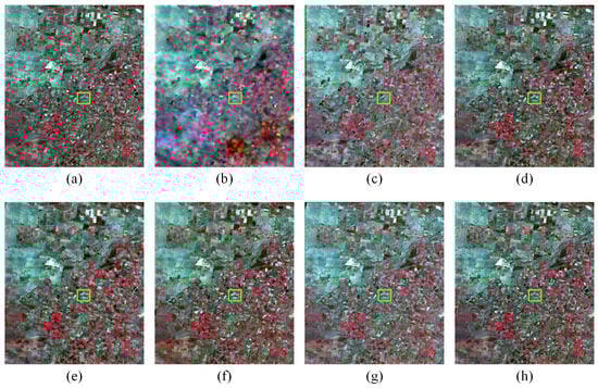
Figure 7.
Example images of the fusion results in the CIA dataset on 17 April 2002. (a) Ground Truth. (b) STARFM. (c) FSDAF. (d) EDCSTFN. (e) GAN-STFM. (f) MLFF-GAN. (g) STM-STFNet. (h) Ours.
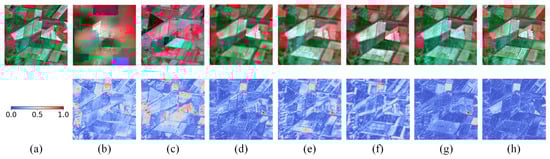
Figure 8.
The first row is an enlarged view of the green rectangular area in Figure 7, and the second row is the absolute average residual maps between the enlarged view and the ground truth. (a) Ground truth. (b) STARFM. (c) FSDAF. (d) EDCSTFN. (e) GAN-STFM. (f) MLFF-GAN. (g) STM-STFNet. (h) Ours.
3.3.2. LGC Dataset Result
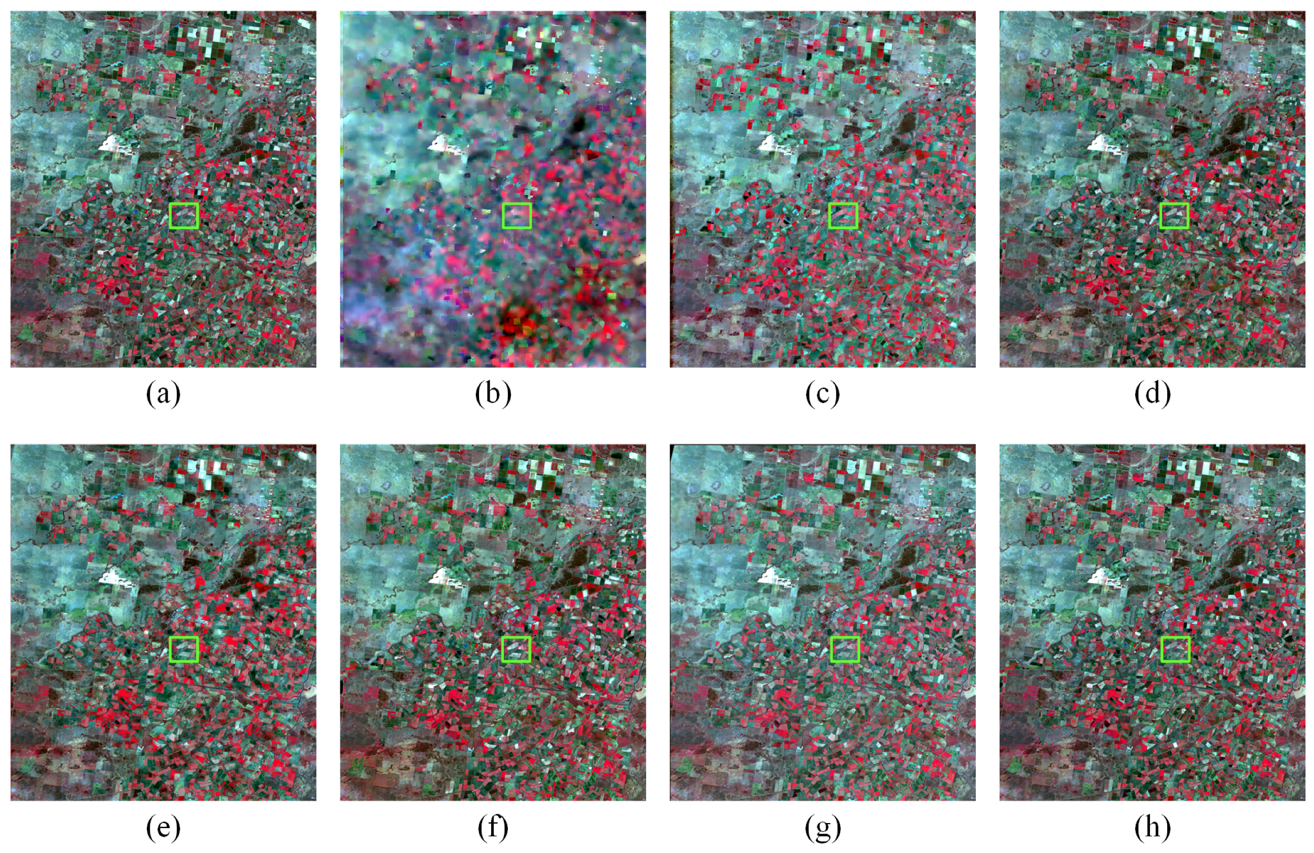
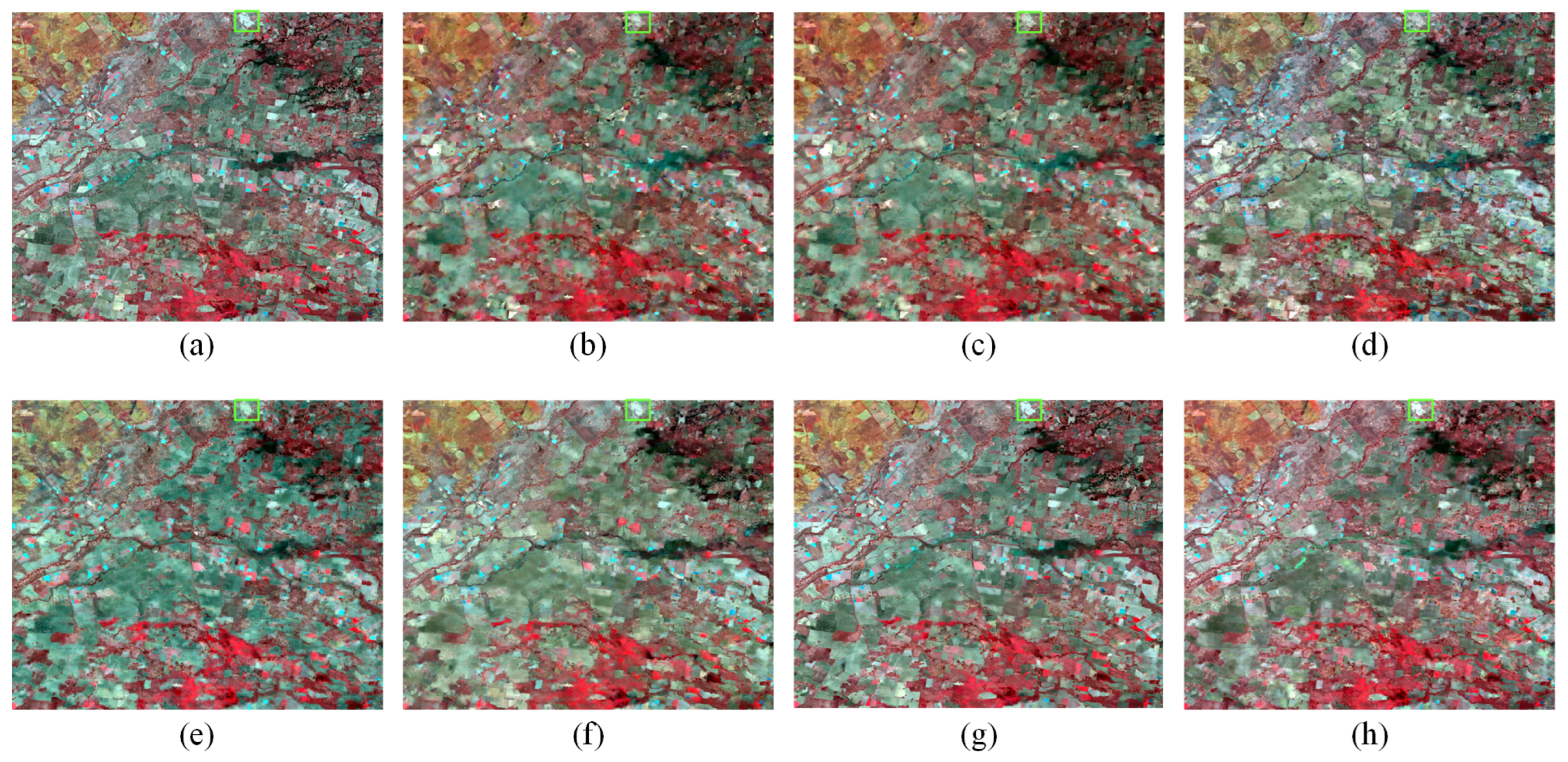
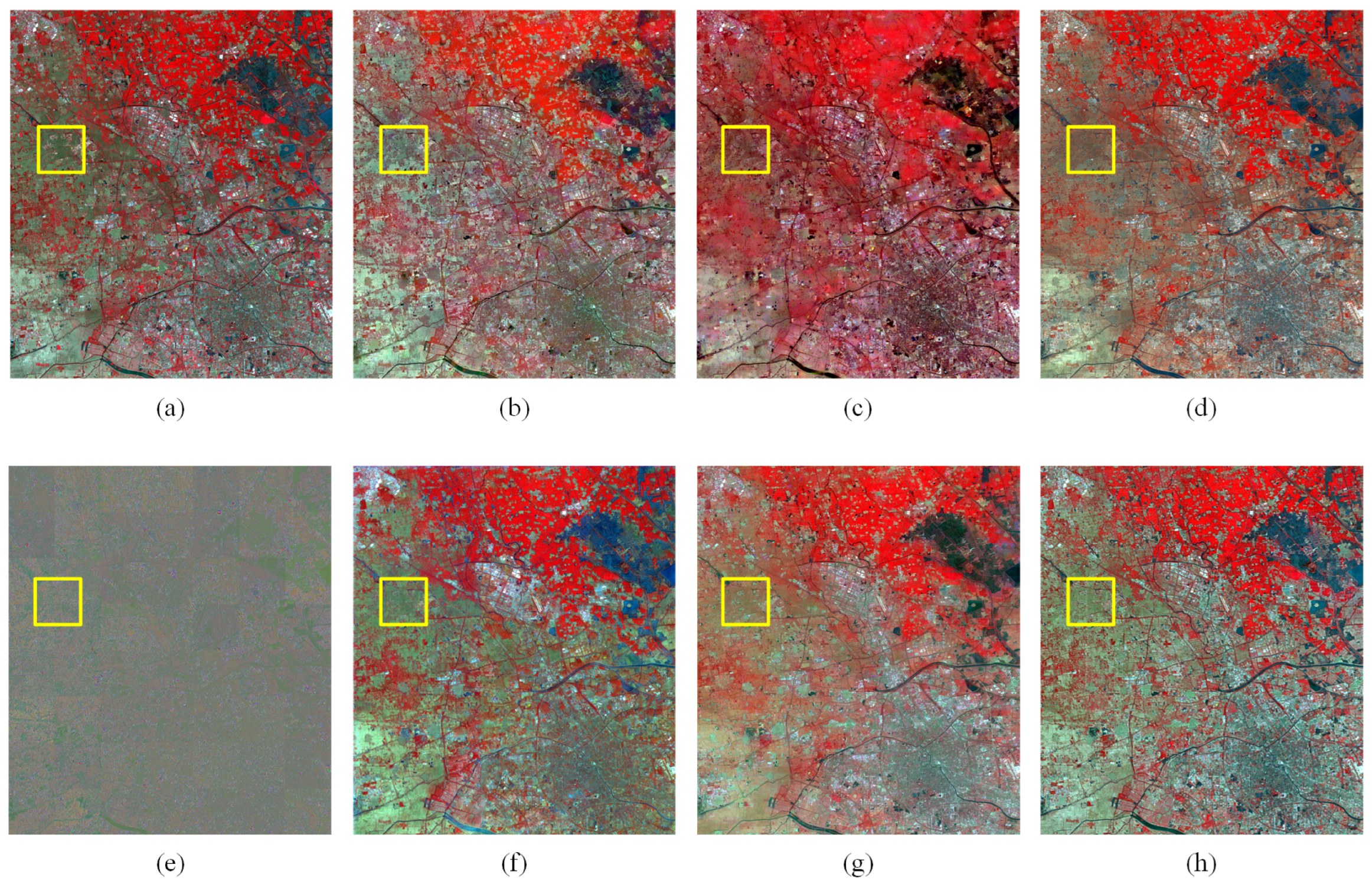
Figure 9 shows the fusion results on the LGC dataset, where traditional methods exhibit noticeable spatial structure distortions in the fused images. As shown in Table 2, the proposed method demonstrates superior overall performance, achieving competitive results across most evaluation metrics, with particularly notable improvements in SAM and SSIM, significantly outperforming traditional methods. Compared to the CIA dataset, all methods achieve significantly better performance on the LGC dataset. In terms of spectral and structural fidelity, the proposed method achieves significantly better SAM and SSIM scores than MLFF-GAN and STM-STFNet, indicating its superior ability to preserve spectral characteristics and spatial details. Although STM-STFNet performs well overall, particularly in RMSE, this advantage is mainly due to the use of a larger number of reference images. As illustrated in Figure 10, the fusion results generated by STARFM and FSDAF exhibit severe spectral distortion. Although deep learning-based spatiotemporal fusion methods alleviate this issue to some extent, varying levels of spectral distortion still remain. The SFT-GAN not only preserves spatial details but also substantially reduces spectral distortion. In summary, the proposed method maintains robust performance under significant land cover changes, demonstrating excellent fusion capability and strong generalizability.

Figure 9.
Example images of the fusion results in the LGC dataset on 26 November 2004. (a) Ground Truth. (b) STARFM, (c) FSDAF, (d) EDCSTFN, (e) GAN-STFM, (f) MLFF-GAN, (g) STM-STFNet, (h) Ours.
Table 2.
Results of contrast experiment on LGC dataset (the best is marked in bold, and the second-best is marked in underline).
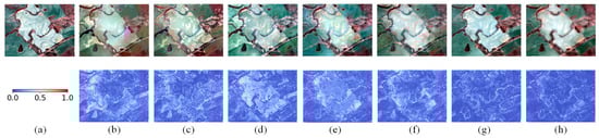
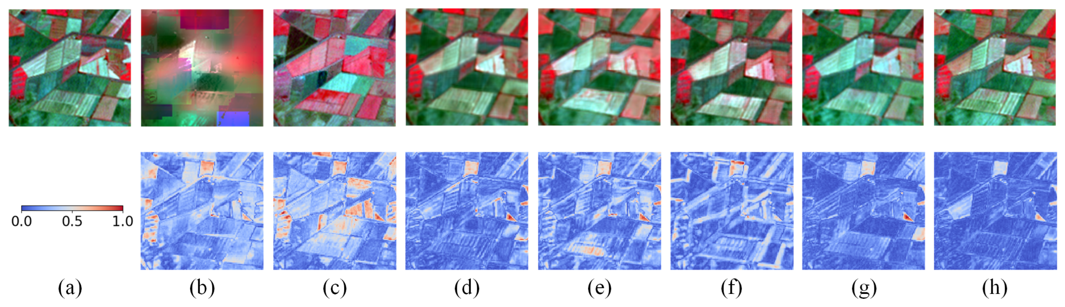
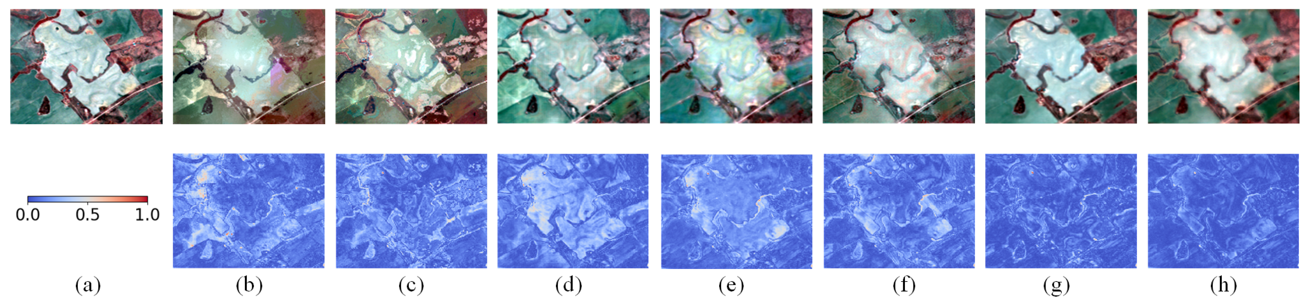
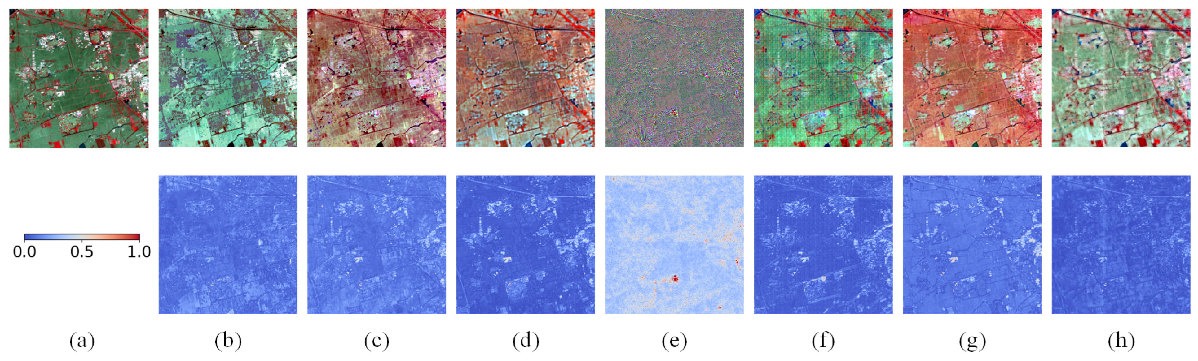
Figure 10.
The first row is an enlarged view of the green rectangular area in Figure 9, and the second row is the absolute average residual maps between the enlarged view and the ground truth. (a) Ground truth. (b) STARFM. (c) FSDAF. (d) EDCSTFN. (e) GAN-STFM. (f) MLFF-GAN. (g) STM-STFNet. (h) Ours.
3.3.3. AHB Dataset Result
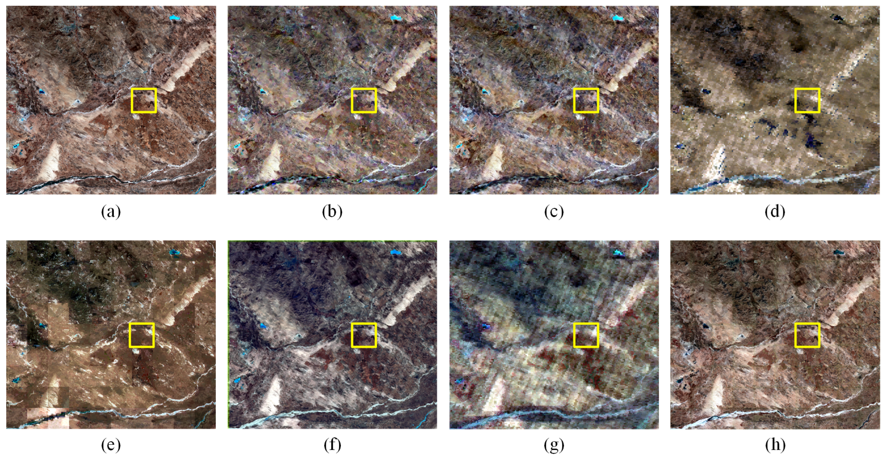
As shown by the evaluation metrics in Table 3, the fusion performance of all methods declined on the AHB dataset compared to the previous two datasets, with traditional methods exhibiting the most significant performance degradation. Nevertheless, the SFT-GAN consistently achieved the best performance across all evaluation metrics. As illustrated in Figure 11, the fusion results from EDCSTFN, MLFF-GAN, and STM-STFNet were significantly affected by noise, with MLFF-GAN and STM-STFNet exhibiting particularly severe spectral distortions. Moreover, none of the compared methods accurately captured the spatiotemporal dynamics of river features. In the magnified views presented in Figure 12, both EDCSTFN and GAN-STFM failed to preserve the structural integrity of circular farmlands. The fusion results generated by the proposed method exhibited the lowest average pixel error and lacked any noticeable abrupt error spikes. Although STM-STFNet achieved a below-average error rate, it still exhibited regions with substantial local errors. In contrast, other methods not only produced higher average errors but also exhibited more severe and frequent error spikes. In summary, the proposed method maintains superior performance even under substantial spectral variations in surface features, further demonstrating its robustness and strong generalizability in complex spatiotemporal fusion scenarios.
Table 3.
Results of contrast experiment on AHB dataset (the best is marked in bold, and the second best is marked in underline).
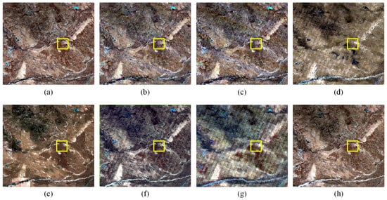
Figure 11.
Example images of the fusion results in the AHB dataset on 17 March 2015. (a) Ground Truth. (b) STARFM. (c) FSDAF. (d) EDCSTFN. (e) GAN-STFM. (f) MLFF-GAN. (g) STM-STFNet. (h) Ours.
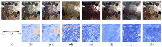
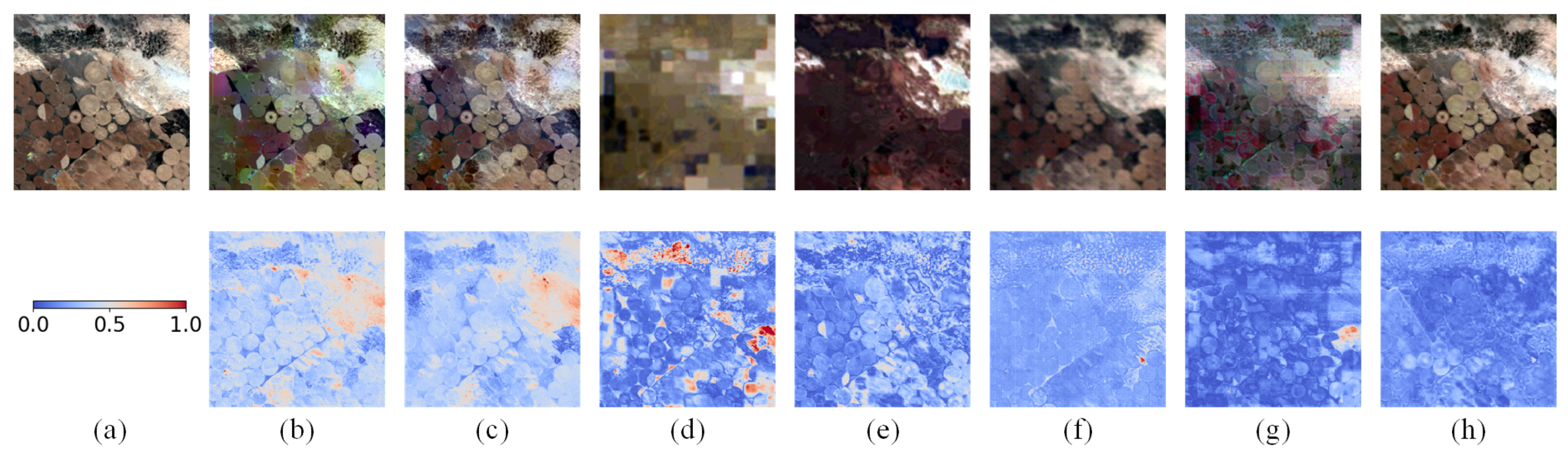
Figure 12.
The first row is an enlarged view of the yellow rectangular area in Figure 11, and the second row is the absolute average residual maps between the enlarged view and the ground truth. (a) Ground truth. (b) STARFM. (c) FSDAF. (d) EDCSTFN. (e) GAN-STFM. (f) MLFF-GAN. (g) STM-STFNet. (h) Ours.
3.3.4. Tianjin Dataset Result
As shown in Table 4, compared to the CIA and LGC datasets, all methods exhibited reduced fusion performance on the Tianjin dataset across quantitative metrics, indicating that this dataset imposes greater demands on method generalization and robustness. Nevertheless, the SFT-GAN consistently achieved the best or second-best performance across most key metrics, with particularly notable results in the SAM index. As illustrated in Figure 13, GAN-STFM produced the poorest fusion results, and FSDAF exhibited severe spectral distortion. EDCSTFN failed to preserve fine details, while STM-STFNet suffered from both significant texture loss and spectral distortion. Local visualizations in Figure 14 further confirm that all methods suffered from varying degrees of spectral distortion. Although MLFF-GAN produced visually appealing results, noticeable noise degraded its performance, resulting in suboptimal quantitative scores. As shown in the absolute average residual maps in Figure 14, the proposed method achieved the lowest average error. Although MLFF-GAN and EDCSTFN also performed relatively well, their results showed noticeable local errors. Overall, the proposed method demonstrated superior performance in handling urban phenological changes. It effectively mitigated the spectral distortion typically observed in traditional methods under complex urban conditions and alleviated the blurring of local details common in deep learning-based models. These results highlight the strong generalization capability and robustness of the proposed approach. These findings also underscore a key limitation of data-driven deep learning methods: their heavy reliance on training data. When applied to challenging datasets such as AHB or Tianjin—characterized by significant land cover changes and large temporal gaps between image pairs—these methods may experience substantial performance degradation or even complete failure.
Table 4.
Results of contrast experiment on Tianjin dataset (the best is marked in bold, and the second-best is marked in underline).

Figure 13.
Example images of the fusion results in the Tianjin dataset on 18 May 2015. (a) Ground Truth. (b) STARFM. (c) FSDAF. (d) EDCSTFN. (e) GAN-STFM. (f) MLFF-GAN. (g) STM-STFNet. (h) Ours.
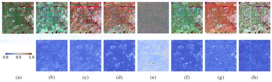
Figure 14.
The first row is an enlarged view of the yellow rectangular area in Figure 13, and the second row is the absolute average residual maps between the enlarged view and the ground truth. (a) Ground truth. (b) STARFM. (c) FSDAF. (d) EDCSTFN. (e) GAN-STFM. (f) MLFF-GAN. (g) STM-STFNet. (h) Ours.
3.3.5. Computational Load
To evaluate computational load, we report the number of parameters, multiply-accumulate operations (MACs), GPU memory usage during training, and training time for each deep learning-based method. MACs indicate the number of multiply-accumulate operations needed to process a six-band image with a resolution of 256 × 256. For GPU memory measurement, we used a batch size of 16 and a patch size of 256 × 256, evaluated on the CIA dataset with all other settings kept at their default values. Time refers to the duration needed to complete a single training epoch. The computational load evaluation results are summarized in Table 5, where Former-GAN denotes a variant of the proposed method with the Sparse Transformer Block replaced by a standard Vision Transformer Block.
Table 5.
Computation load of five deep learning methods (G denotes the generator, D denotes the discriminator).
Among the five deep learning methods, both STM-STFNet and the proposed SFT-GAN are based on the transformer architecture, leading to relatively large parameter counts. However, with the introduction of the Sparse Transformer Block, SFT-GAN significantly reduces computational complexity, achieving the lowest MACs among all methods—approximately 29% of those required by MLFF-GAN. In addition, due to the sparsity mechanism embedded in the Sparse Transformer Block, SFT-GAN achieves the lowest GPU memory usage during training, consuming only 6.72 GiB. This advantage enables the method to process larger-scale remote sensing imagery under identical hardware conditions, effectively reducing dependence on high-performance computing resources. Moreover, SFT-GAN shows superior training efficiency, reducing training time by approximately 80% compared to STM-STFNet. A comparison with Former-GAN further confirms that the Sparse Transformer Block effectively reduces both computational and memory complexities. In summary, SFT-GAN not only significantly reduces computational cost and training time, but also greatly enhances model usability and practicality through sparse optimization strategies. These advantages make it a promising solution for resource-constrained applications, such as onboard processing on unmanned aerial vehicles.
3.3.6. Classification Results of Fusion Images
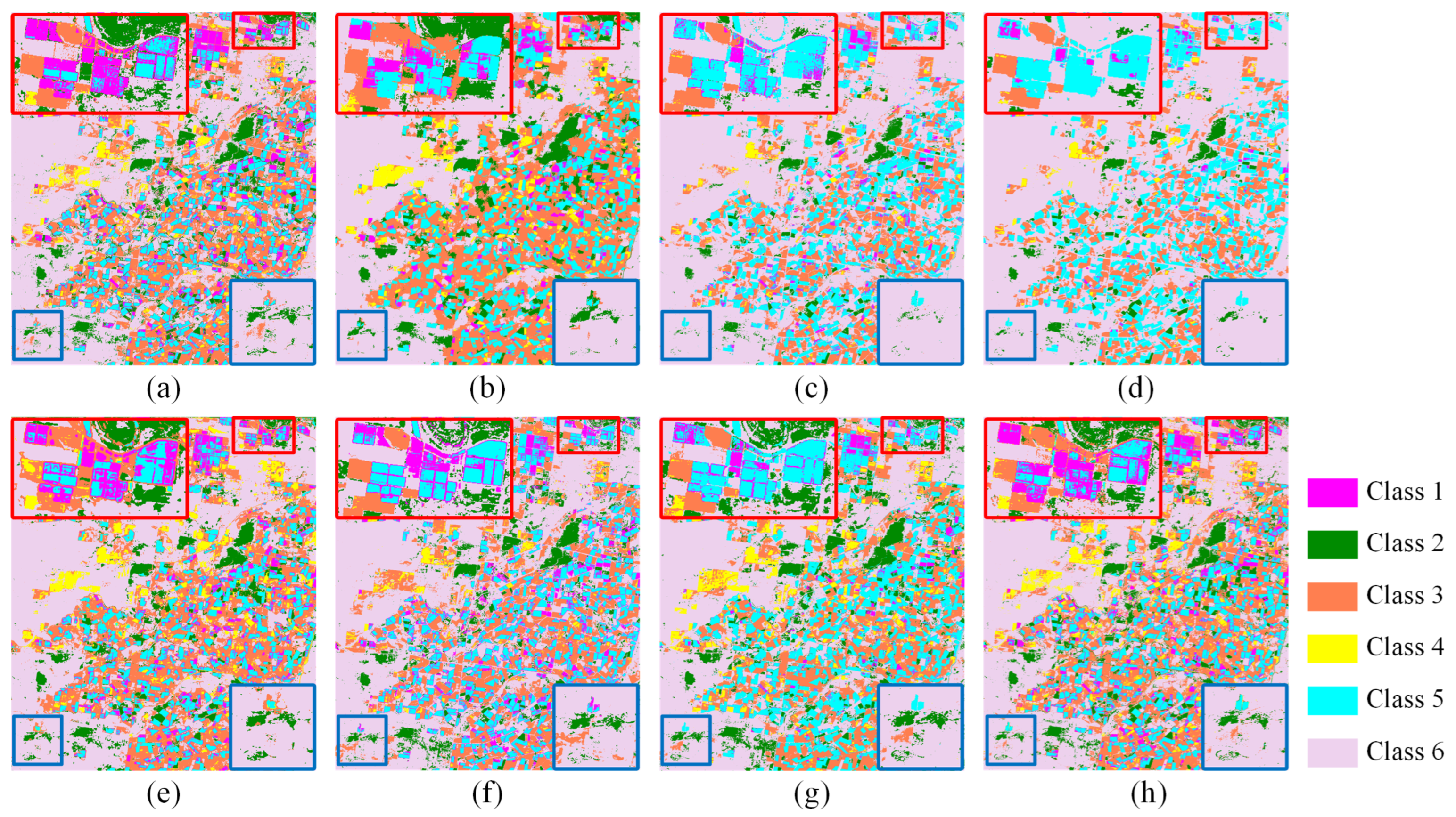
To further validate the practicality of the proposed method, a classification experiment was conducted to assess the quality and usability of the fused images. Specifically, a Support Vector Machine (SVM)-based classifier was used to classify fused images generated from the CIA dataset. As the CIA dataset lacks predefined land cover categories, the images were manually categorized into six land cover types. Classification results from the fused images generated by SFT-GAN and other competing methods were compared with those from true high-resolution images. The results are shown in Figure 15 and summarized in Table 6. The experimental results indicate that the fused images generated by SFT-GAN achieve the highest Overall Accuracy (OA) of 80.89% and a Kappa coefficient of 0.7259, demonstrating superior classification performance. These findings further validate the practical value of SFT-GAN and demonstrate that the proposed modules effectively improve both spectral consistency and spatial detail representation. Consequently, SFT-GAN offers more reliable data for downstream remote sensing tasks such as land cover classification and change detection.
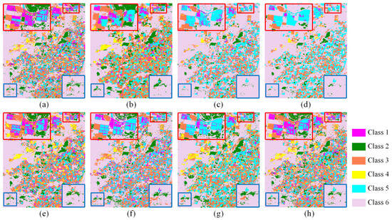
Figure 15.
Example images of classification results in the CIA dataset. (a) Ground truth, (b) STARFM, (c) FSDAF, (d) EDCSTFN, (e) GAN-STFM, (f) MLFF-GAN, (g) STM-STFNet, (h) Ours.
Table 6.
Results of classification experiment on CIA dataset.
3.4. Ablation Study
The ablation study consists of two parts: (1) evaluating the effectiveness of each proposed module in the SFT-GAN framework; (2) assessing the impact of different parameters in the Detail Compensation Module on fused image quality, including a comparison of the Butterworth, ideal, and Gaussian filters. The ablation experiments were conducted on the CIA dataset, focusing on the fused image corresponding to 11 January 2002. During training, the initial learning rate was set to and was reduced by 20% every 10 epochs. The batch size was set to 16, with a total of 500 training epochs.
To evaluate the contributions of the Sparse Transformer Module (STM), Detail Compensation Module (DCM), and Spectrum Compensation Module (SCM), four ablation experiments were conducted: (1) retaining SCM while removing DCM from SFT-GAN; (2) retaining DCM while removing SCM from SFT-GAN; (3) removing both DCM and SCM from SFT-GAN; (4) replacing the STM in SFT-GAN with a standard Vision Transformer.
The ablation study evaluated the effectiveness of multi-module collaboration by comparing the performance of different module combinations. The results are presented in Table 7. When STM, DCM, and SCM are all enabled, the model achieves the best performance across all evaluation metrics. Removing SCM alone significantly increases the SAM value to 3.7743, highlighting the importance of SCM in preserving spectral fidelity. In contrast, removing DCM decreases the SSIM to 0.8631, demonstrating its essential role in fine detail compensation. When only STM is retained, both RMSE and PSNR deteriorate, further confirming the necessity of DCM and SCM collaboration. Notably, replacing STM with a standard Vision Transformer leads to lower PSNR and SSIM compared to the complete model, indicating that STM reduces computational and spatial complexities without sacrificing fusion accuracy. In conclusion, the joint use of STM, DCM, and SCM effectively balances spatial detail enhancement, spectral consistency, and structural similarity, offering a robust solution for multi-source remote sensing image spatiotemporal fusion.
Table 7.
Ablation study results of the modules (the best is marked in bold, and the second-best is marked in underline. ✓ indicates that the module is used, whereas ✗ indicates that it is not).
Additionally, an ablation study was conducted to investigate the impact of different DCM parameters and low-pass filter types. The Butterworth filter was replaced by the Ideal and Gaussian filters. For each filter type, two parameter sets were tested for the Gaussian filter as well as the Ideal filter, and four for the Butterworth filter. The quantitative evaluation results are presented in Table 8. Specifically, for the Butterworth filter, the first parameter is the cutoff frequency , and the second is the filter order n. For the Gaussian filter, the parameter is the standard deviation , while the Ideal filter uses the cutoff frequency as its sole parameter. The Gaussian and Ideal filters are single-parameter filters.
Table 8.
Ablation study results of different filters (the best is marked in bold, and the second-best is marked in underline).
Overall, the Butterworth filter achieves the best performance under the parameter combination (parameter 1 = 50, 150, 250; parameter 2 = 2, 4, 4), particularly in terms of PSNR and SAM. Notably, parameter 2 has a significant impact on spectral fidelity. When parameter 1 is fixed, changing parameter 2 from (2, 4, 4) to (2, 2, 4) leads to a sharp increase in the SAM value to 4.0781, highlighting its strong influence on spectral consistency. In contrast, although the Gaussian filter yields lower RMSE values with parameter 1 = 1, 2, 3, its performance on other metrics is inferior to that of the Butterworth filter. The Ideal filter performs well in terms of SSIM but shows poor results on other metrics. In summary, the Butterworth filter provides the best trade-off between spatial detail preservation, spectral accuracy, and structural consistency, making it the optimal filter choice for the DCM.
3.5. Stability Study
To evaluate the stability of the proposed model, a stability experiment was designed. Based on the CIA dataset, a total of 15 image pairs were selected, and 10 random experiments were conducted. In each experiment, 3 image pairs were randomly chosen as the test set, and the remaining 12 pairs were used for training. The results on the test set were averaged in each round to obtain the final result for that experiment. RMSE, SSIM, SAM, ERGAS, PSNR, and UIQI were used as evaluation metrics. The standard deviation of each metric across the 10 experiments was calculated to assess the model’s performance stability. The results are summarized in Table 9.
Table 9.
Result of random experiments.
Table 9 reports the mean and standard deviation of each performance metric across the 10 randomized experiments. As shown in the results, UIQI and SSIM exhibit relatively low standard deviations, indicating that the proposed method is stable in reconstructing structural information. In contrast, the standard deviation of SAM is relatively high, suggesting that the spectral reconstruction performance is somewhat sensitive to the composition of the training samples. Overall, although the model exhibits a certain degree of variation across multiple experiments, the range of performance fluctuations remains within a reasonable and acceptable interval, indicating that the proposed method possesses stability.
4. Discussion
To overcome the limitations of existing deep learning-based multi-source remote sensing spatiotemporal fusion methods, this article proposes a novel approach based on GAN and sparse transformer. The generator consists of three main stages: feature extraction, feature fusion, and information compensation. In the feature extraction stage, a Sparse Transformer Module is applied to reduce computational complexity while preserving the model’s feature extraction capability. During feature fusion, the Feature Reconstruction Module leverages a channel attention mechanism to flexibly integrate spatial detail and temporal variation features. In the information compensation stage, the Detail Compensation Module applies frequency-domain decomposition to recover high-frequency details, thereby enhancing spatial fidelity. Meanwhile, the Spectrum Compensation Module improves spectral fidelity by incorporating band correlation constraints.
Through this multi-stage design, the proposed method achieves an effective trade-off between spectral fidelity, spatial detail preservation, and computational efficiency. Notably, comparative experiments on four benchmark datasets demonstrate that Sparse Fast Transformer fusion method based on Generative Adversarial Network (SFT-GAN) consistently outperforms existing state-of-the-art methods in both quantitative metrics and visual quality. Moreover, ablation studies validate the individual contributions of each component, particularly highlighting the importance of detail compensation and spectrum compensation in preserving fine-grained spatial and spectral information. Despite these promising results, certain limitations remain. The model may exhibit reduced robustness under extreme atmospheric conditions or abrupt land cover changes, such as the result in the Tianjin dataset.
5. Conclusions
This study addresses the persistent challenges in multi-source remote sensing spatiotemporal fusion, including insufficient spectral fidelity and high computational complexity. To this end, we propose the Sparse Fast Transformer fusion method based on Generative Adversarial Network (SFT-GAN), a novel fusion framework that integrates a sparse transformer-based generator with specialized compensation modules for detail and spectral restoration. Through a sparse optimization strategy, the model significantly reduces computational overhead, making it suitable for resource-constrained platforms such as UAVs. Experimental results on four diverse public datasets demonstrate that SFT-GAN achieves superior fusion accuracy and generalization capability across varying spatial and temporal scenarios.
In particular, the proposed Spectrum Compensation Module markedly enhances spectral fidelity, ensuring the applicability of the fused images in downstream tasks such as land use monitoring and ecological environment assessment. Overall, the method strikes an effective balance between accuracy and efficiency, representing a practical solution for real-world remote sensing applications.
However, the proposed method still has certain limitations. The performance of SFT-GAN may decline when land cover types undergo drastic changes. Future research will focus on further optimizing the network architecture to enhance its adaptability under complex land cover change conditions. Currently, most existing fusion methods adopt an early fusion strategy, namely feature-level fusion. Future research will further explore the potential of late fusion strategies [57] in the spatiotemporal fusion of remote sensing images, aiming to enhance fusion performance and improve model generalization. Additionally, we will investigate the integration of spectral physical priors into deep learning models to further enhance the spectral fidelity of fused images. Currently, most standard benchmark datasets are based on Landsat-MODIS data. To further validate the generalization capability of the model, we plan to incorporate data from other types of sensors (e.g., Gaofen-1) into spatiotemporal fusion studies, which will be one of the key directions in our future work.
Author Contributions
Conceptualization, Z.M. and W.B.; methodology, Z.M.; software, Z.M.; validation, Z.M. and W.B.; formal analysis, Z.M. and W.B.; investigation, Z.M. and W.B.; resources, W.B., X.Z. and X.M.; data curation, W.B., X.Z., X.M. and K.Q.; writing—original draft preparation, Z.M.; writing—review and editing, W.B. and W.F.; visualization, Z.M.; supervision, W.B.; project administration, W.B.; funding acquisition, W.B. All authors have read and agreed to the published version of the manuscript.
Funding
This work was supported by the Natural Science Foundation of Ningxia Province of China (Grant number 2024AAC02035), the National Natural Science Foundation of China (grant numbers 62461001, 62201438), and the Image and Intelligence Information Processing Innovation Team of the National Ethnic Affairs Commission of China.
Data Availability Statement
The original contributions presented in this study are included in the article. Further inquiries can be directed to the corresponding author.
Conflicts of Interest
The authors declare no conflicts of interest.
References
- Weiss, M.; Jacob, F.; Duveiller, G. Remote sensing for agricultural applications: A meta-review. Remote Sens. Environ. 2020, 236, 111402. [Google Scholar] [CrossRef]
- Zhang, W.; Guo, S.; Zhang, P.; Xia, Z.; Zhang, X.; Lin, C.; Tang, P.; Fang, H.; Du, P. A Novel Knowledge-Driven Automated Solution for High-Resolution Cropland Extraction by Cross-Scale Sample Transfer. IEEE Trans. Geosci. Remote Sens. 2023, 61, 1–16. [Google Scholar] [CrossRef]
- Zhou, X.; Wang, T.; Zheng, W.; Zhang, M.; Wang, Y. Reconstruction of Fine-Spatial-Resolution FY-3D-Based Vegetation Indices to Achieve Farmland-Scale Winter Wheat Yield Estimation via Fusion with Sentinel-2 Data. Remote Sens. 2024, 16, 4143. [Google Scholar] [CrossRef]
- Zhang, F.; Duan, P.; Jim, C.Y.; Johnson, V.C.; Liu, C.; Chan, N.W.; Tan, M.L.; Kung, H.T.; Shi, J.; Wang, W. An advanced spatiotemporal fusion model for suspended particulate matter monitoring in an intermontane lake. Remote Sens. 2023, 15, 1204. [Google Scholar] [CrossRef]
- Tang, R.; Wei, X.; Chen, C.; Jiang, R.; Shen, F. Remote Sensing Observations of a Coastal Water Environment Based on Neural Network and Spatiotemporal Fusion Technology: A Case Study of Hangzhou Bay. Remote Sens. 2024, 16, 800. [Google Scholar] [CrossRef]
- Tan, Y.; Sun, K.; Wei, J.; Gao, S.; Cui, W.; Duan, Y.; Liu, J.; Zhou, W. STFNet: A Spatiotemporal Fusion Network for Forest Change Detection Using Multi-Source Satellite Images. Remote Sens. 2024, 16, 4736. [Google Scholar] [CrossRef]
- Hong, Y.; Zhou, R.; Liu, J.; Que, X.; Chen, B.; Chen, K.; He, Z.; Huang, G. Monitoring Mangrove Phenology Based on Gap Filling and Spatiotemporal Fusion: An Optimized Mangrove Phenology Extraction Approach (OMPEA). Remote Sens. 2025, 17, 549. [Google Scholar] [CrossRef]
- Wu, Z.; Shi, F. Mapping Forest Canopy Height at Large Scales Using ICESat-2 and Landsat: An Ecological Zoning Random Forest Approach. IEEE Trans. Geosci. Remote Sens. 2023, 61, 1–16. [Google Scholar] [CrossRef]
- Bai, Z.; Han, L.; Jiang, X.; Liu, M.; Li, L.; Liu, H.; Lu, J. Spatiotemporal evolution of desertification based on integrated remote sensing indices in Duolun County, Inner Mongolia. Ecol. Inform. 2022, 70, 101750. [Google Scholar] [CrossRef]
- Song, Z.; Lu, Y.; Yuan, J.; Lu, M.; Qin, Y.; Sun, D.; Ding, Z. Research on Desertification Monitoring and Vegetation Refinement Extraction Methods Based on the Synergy of Multi-Source Remote Sensing Imagery. IEEE Trans. Geosci. Remote Sens. 2025, 63, 4404819. [Google Scholar] [CrossRef]
- Ran, L.; Zhang, L.; He, Y.; Cao, S.; Ding, Y.; Guo, Y.; Wei, X.; Filonchyk, M. Spatiotemporal Dynamic Change and the Driving Mechanism of Desertification in the Yellow River Basin. IEEE J. Sel. Top. Appl. Earth Obs. Remote Sens. 2024, 17, 17134–17155. [Google Scholar] [CrossRef]
- Wang, Q.; Tang, Y.; Ge, Y.; Xie, H.; Tong, X.; Atkinson, P.M. A comprehensive review of spatial-temporal-spectral information reconstruction techniques. Sci. Remote Sens. 2023, 8, 100102. [Google Scholar] [CrossRef]
- Zhu, X.; Cai, F.; Tian, J.; Williams, T.K.A. Spatiotemporal fusion of multisource remote sensing data: Literature survey, taxonomy, principles, applications, and future directions. Remote Sens. 2018, 10, 527. [Google Scholar] [CrossRef]
- Zhu, X.; Chen, J.; Gao, F.; Chen, X.; Masek, J.G. An enhanced spatial and temporal adaptive reflectance fusion model for complex heterogeneous regions. Remote Sens. Environ. 2010, 114, 2610–2623. [Google Scholar] [CrossRef]
- Gao, F.; Masek, J.; Schwaller, M.; Hall, F. On the blending of the Landsat and MODIS surface reflectance: Predicting daily Landsat surface reflectance. IEEE Trans. Geosci. Remote Sens. 2006, 44, 2207–2218. [Google Scholar] [CrossRef]
- Xu, C.; Du, X.; Fan, X.; Jian, H.; Yan, Z.; Zhu, J.; Wang, R. FastVSDF: An Efficient Spatiotemporal Data Fusion Method for Seamless Data Cube. IEEE Trans. Geosci. Remote Sens. 2024, 62, 1–22. [Google Scholar] [CrossRef]
- Hou, S.; Sun, W.; Guo, B.; Li, C.; Li, X.; Shao, Y.; Zhang, J. Adaptive-SFSDAF for spatiotemporal image fusion that selectively uses class abundance change information. Remote Sens. 2020, 12, 3979. [Google Scholar] [CrossRef]
- Zhu, X.; Helmer, E.H.; Gao, F.; Liu, D.; Chen, J.; Lefsky, M.A. A flexible spatiotemporal method for fusing satellite images with different resolutions. Remote Sens. Environ. 2016, 172, 165–177. [Google Scholar] [CrossRef]
- Huang, B.; Song, H. Spatiotemporal Reflectance Fusion via Sparse Representation. IEEE Trans. Geosci. Remote Sens. 2012, 50, 3707–3716. [Google Scholar] [CrossRef]
- Wu, B.; Huang, B.; Zhang, L. An error-bound-regularized sparse coding for spatiotemporal reflectance fusion. IEEE Trans. Geosci. Remote Sens. 2015, 53, 6791–6803. [Google Scholar] [CrossRef]
- Lian, Z.; Zhan, Y.; Zhang, W.; Wang, Z.; Liu, W.; Huang, X. Recent Advances in Deep Learning-Based Spatiotemporal Fusion Methods for Remote Sensing Images. Sensors 2025, 25, 1093. [Google Scholar] [CrossRef] [PubMed]
- Goodfellow, I.J.; Pouget-Abadie, J.; Mirza, M.; Xu, B.; Warde-Farley, D.; Ozair, S.; Courville, A.; Bengio, Y. Generative Adversarial Nets. In Proceedings of the Advances in Neural Information Processing Systems, Montreal, QC, USA, 8–13 December 2014; Ghahramani, Z., Welling, M., Cortes, C., Lawrence, N., Weinberger, K., Eds.; Curran Associates, Inc.: New York, NY, USA, 2014; Volume 27. [Google Scholar]
- Salazar, A.; Vergara, L.; Safont, G. Generative Adversarial Networks and Markov Random Fields for oversampling very small training sets. Expert Syst. Appl. 2021, 163, 113819. [Google Scholar] [CrossRef]
- Lyu, F.; Yang, Z.; Diao, C.; Wang, S. Multi-stream STGAN: A Spatiotemporal Image Fusion Model with Improved Temporal Transferability. IEEE J. Sel. Top. Appl. Earth Obs. Remote Sens. 2024, 18, 1562–1576. [Google Scholar] [CrossRef]
- Weng, C.; Zhan, Y.; Gu, X.; Yang, J.; Liu, Y.; Guo, H.; Lian, Z.; Zhang, S.; Wang, Z.; Zhao, X. The Spatially Seamless Spatiotemporal Fusion Model Based on Generative Adversarial Networks. IEEE J. Sel. Top. Appl. Earth Obs. Remote Sens. 2024, 17, 12760–12771. [Google Scholar] [CrossRef]
- Liu, H.; Yang, G.; Deng, F.; Qian, Y.; Fan, Y. MCBAM-GAN: The GAN spatiotemporal fusion model based on multiscale and CBAM for remote sensing images. Remote Sens. 2023, 15, 1583. [Google Scholar] [CrossRef]
- Tan, Z.; Gao, M.; Li, X.; Jiang, L. A flexible reference-insensitive spatiotemporal fusion model for remote sensing images using conditional generative adversarial network. IEEE Trans. Geosci. Remote Sens. 2021, 60, 1–13. [Google Scholar] [CrossRef]
- Liu, Q.; Meng, X.; Shao, F.; Li, S. PSTAF-GAN: Progressive spatio-temporal attention fusion method based on generative adversarial network. IEEE Trans. Geosci. Remote Sens. 2022, 60, 1–13. [Google Scholar] [CrossRef]
- Song, B.; Liu, P.; Li, J.; Wang, L.; Zhang, L.; He, G.; Chen, L.; Liu, J. MLFF-GAN: A multilevel feature fusion with GAN for spatiotemporal remote sensing images. IEEE Trans. Geosci. Remote Sens. 2022, 60, 1–16. [Google Scholar] [CrossRef]
- Lei, D.; Zhu, Q.; Li, Y.; Tan, J.; Wang, S.; Zhou, T.; Zhang, L. HPLTS-GAN: A High-Precision Remote Sensing Spatio-Temporal Fusion Method Based on Low Temporal Sensitivity. IEEE Trans. Geosci. Remote Sens. 2024, 62, 5407416. [Google Scholar] [CrossRef]
- Zhang, X.; Li, S.; Tan, Z.; Li, X. Enhanced wavelet based spatiotemporal fusion networks using cross-paired remote sensing images. ISPRS J. Photogramm. Remote Sens. 2024, 211, 281–297. [Google Scholar] [CrossRef]
- Lei, D.; Ran, G.; Zhang, L.; Li, W. A spatiotemporal fusion method based on multiscale feature extraction and spatial channel attention mechanism. Remote Sens. 2022, 14, 461. [Google Scholar] [CrossRef]
- Zheng, X.; Feng, R.; Fan, J.; Han, W.; Yu, S.; Chen, J. Msisr-stf: Spatiotemporal fusion via multilevel single-image super-resolution. Remote Sens. 2023, 15, 5675. [Google Scholar] [CrossRef]
- Yang, Z.; Diao, C.; Li, B. A robust hybrid deep learning model for spatiotemporal image fusion. Remote Sens. 2021, 13, 5005. [Google Scholar] [CrossRef]
- Tan, Z.; Di, L.; Zhang, M.; Guo, L.; Gao, M. An enhanced deep convolutional model for spatiotemporal image fusion. Remote Sens. 2019, 11, 2898. [Google Scholar] [CrossRef]
- Jiang, H.; Qian, Y.; Yang, G.; Liu, H. MLKNet: Multi-Stage for Remote Sensing Image Spatiotemporal Fusion Network Based on a Large Kernel Attention. IEEE J. Sel. Top. Appl. Earth Obs. Remote Sens. 2024, 17, 1257–1268. [Google Scholar] [CrossRef]
- You, M.; Meng, X.; Liu, Q.; Shao, F.; Fu, R. CIG-STF: Change Information Guided Spatio-temporal Fusion for Remote Sensing Images. IEEE Trans. Geosci. Remote Sens. 2024, 62, 5405815. [Google Scholar] [CrossRef]
- Dosovitskiy, A. An image is worth 16x16 words: Transformers for image recognition at scale. arXiv 2020, arXiv:2010.11929. [Google Scholar]
- Aleissaee, A.A.; Kumar, A.; Anwer, R.M.; Khan, S.; Cholakkal, H.; Xia, G.S.; Khan, F.S. Transformers in remote sensing: A survey. Remote Sens. 2023, 15, 1860. [Google Scholar] [CrossRef]
- Benzenati, T.; Kallel, A.; Kessentini, Y. STF-Trans: A two-stream spatiotemporal fusion transformer for very high resolution satellites images. Neurocomputing 2024, 563, 126868. [Google Scholar] [CrossRef]
- Li, W.; Cao, D.; Peng, Y.; Yang, C. MSNet: A multi-stream fusion network for remote sensing spatiotemporal fusion based on transformer and convolution. Remote Sens. 2021, 13, 3724. [Google Scholar] [CrossRef]
- Wang, S.; Fan, F. STINet: Vegetation Changes Reconstruction through a Transformer-based Spatiotemporal Fusion Approach in Remote Sensing. IEEE Trans. Geosci. Remote Sens. 2024, 62, 4412116. [Google Scholar] [CrossRef]
- Qian, Z.; Yue, L.; Xie, X.; Yuan, Q.; Shen, H. A Dual-Perspective Spatio-Temporal Fusion Model for Remote Sensing Images by Discriminative Learning of the Spatial and Temporal Mapping. IEEE J. Sel. Top. Appl. Earth Obs. Remote Sens. 2024, 17, 12505–12520. [Google Scholar] [CrossRef]
- Chen, G.; Jiao, P.; Hu, Q.; Xiao, L.; Ye, Z. SwinSTFM: Remote sensing spatiotemporal fusion using Swin transformer. IEEE Trans. Geosci. Remote Sens. 2022, 60, 1–18. [Google Scholar] [CrossRef]
- Child, R.; Gray, S.; Radford, A.; Sutskever, I. Generating long sequences with sparse transformers. arXiv 2019, arXiv:1904.10509. [Google Scholar]
- Zhang, Q.; Yang, Y.B. ResT: An Efficient Transformer for Visual Recognition. In Proceedings of the Advances in Neural Information Processing Systems, Online, 6–14 December 2021; Ranzato, M., Beygelzimer, A., Dauphin, Y., Liang, P., Vaughan, J.W., Eds.; Curran Associates, Inc.: New York, NY, USA, 2021; Volume 34, pp. 15475–15485. [Google Scholar]
- Lin, T.; Wang, Y.; Liu, X.; Qiu, X. A survey of transformers. AI Open 2022, 3, 111–132. [Google Scholar] [CrossRef]
- Vaswani, A.; Shazeer, N.; Parmar, N.; Uszkoreit, J.; Jones, L.; Gomez, A.N.; Kaiser, L.U.; Polosukhin, I. Attention is All you Need. In Proceedings of the Advances in Neural Information Processing Systems, Long Beach, CA, USA, 4–9 December 2017; Guyon, I., Luxburg, U.V., Bengio, S., Wallach, H., Fergus, R., Vishwanathan, S., Garnett, R., Eds.; Curran Associates, Inc.: New York, NY, USA, 2017; Volume 30. [Google Scholar]
- Pan, Z.; Yu, W.; Wang, B.; Xie, H.; Sheng, V.S.; Lei, J.; Kwong, S. Loss functions of generative adversarial networks (GANs): Opportunities and challenges. IEEE Trans. Emerg. Top. Comput. Intell. 2020, 4, 500–522. [Google Scholar] [CrossRef]
- Mao, X.; Li, Q.; Xie, H.; Lau, R.Y.; Wang, Z.; Paul Smolley, S. Least squares generative adversarial networks. In Proceedings of the IEEE international Conference on Computer Vision, Venice, Italy, 22–29 October 2017; pp. 2794–2802. [Google Scholar]
- Emelyanova, I.V.; McVicar, T.R.; Van Niel, T.G.; Li, L.T.; Van Dijk, A.I. Assessing the accuracy of blending Landsat–MODIS surface reflectances in two landscapes with contrasting spatial and temporal dynamics: A framework for algorithm selection. Remote Sens. Environ. 2013, 133, 193–209. [Google Scholar] [CrossRef]
- Li, J.; Li, Y.; He, L.; Chen, J.; Plaza, A. Spatio-temporal fusion for remote sensing data: An overview and new benchmark. Sci. China Inf. Sci. 2020, 63, 1–17. [Google Scholar] [CrossRef]
- Khan, M.M.; Alparone, L.; Chanussot, J. Pansharpening quality assessment using the modulation transfer functions of instruments. IEEE Trans. Geosci. Remote Sens. 2009, 47, 3880–3891. [Google Scholar] [CrossRef]
- Yuhas, R.H.; Goetz, A.F.; Boardman, J.W. Discrimination among semi-arid landscape endmembers using the spectral angle mapper (SAM) algorithm. In Proceedings of the JPL, Summaries of the Third Annual JPL Airborne Geoscience Workshop, Pasadena, CA, USA, 1–5 June 1992; Volume 1. [Google Scholar]
- Wang, Z.; Bovik, A.C.; Sheikh, H.R.; Simoncelli, E.P. Image quality assessment: From error visibility to structural similarity. IEEE Trans. Image Process. 2004, 13, 600–612. [Google Scholar] [CrossRef]
- Wang, Z.; Bovik, A.C. A universal image quality index. IEEE Signal Process. Lett. 2002, 9, 81–84. [Google Scholar] [CrossRef]
- Vergara, L.; Salazar, A. On the Optimum Linear Soft Fusion of Classifiers. Appl. Sci. 2025, 15, 5038. [Google Scholar] [CrossRef]


Disclaimer/Publisher’s Note: The statements, opinions and data contained in all publications are solely those of the individual author(s) and contributor(s) and not of MDPI and/or the editor(s). MDPI and/or the editor(s) disclaim responsibility for any injury to people or property resulting from any ideas, methods, instructions or products referred to in the content. |
© 2025 by the authors. Licensee MDPI, Basel, Switzerland. This article is an open access article distributed under the terms and conditions of the Creative Commons Attribution (CC BY) license (https://creativecommons.org/licenses/by/4.0/).