Multi-Temporal Dual Polarimetric SAR Crop Classification Based on Spatial Information Comprehensive Utilization

Abstract

Dual polarimetric SAR is capable of reflecting the biophysical and geometrical information of terrain with open access data availability. When it is combined with time-series observations, it can effectively capture the dynamic evolution of scattering characteristics of crops in different growth cycles. However, the actual planting of crops often shows spatial dispersion, and the same crop may be dispersed in different plots, which fails to adequately consider the correlation information between dispersed plots of the same crop in spatial distribution. This study proposed a crop classification method based on multi-temporal dual polarimetric data, which considered the utilization of information between near and far spatial plots, by employing superpixel segmentation and a HyperGraph neural network, respectively. Firstly, the method utilized the dual polarimetric covariance matrix of multi-temporal data to perform superpixel segmentation on neighboring pixels, so that the segmented superpixel blocks were highly compatible with the actual plot shapes from a long-term period perspective. Then, a HyperGraph adjacency matrix was constructed, and a HyperGraph neural network (HGNN) was utilized to better learn the features of plots of the same crop that are distributed far from each other. The method fully utilizes the three dimensions of time, polarization and space information, which complement each other so as to effectively realize high-precision crop classification. The Sentinel-1 experimental results show that, under the optimal parameter settings, the classified accuracy of combined temporal superpixel scattering features using the HGNN was obviously improved, considering the near and far distance spatial correlations of crop types.

1. Introduction

Synthetic Aperture Radar (SAR) is an active microwave remote sensing technology. Due to its unique working principle, it has the capability of all-day, all-weather observation and high-resolution imaging [1]. It is able to penetrate the cloud layer and part of the vegetation cover to obtain information on the scattering characteristics of terrains. Among the existing space-borne SAR systems, dual polarimetric SAR has become an important data source in the field of agricultural monitoring due to its comprehensive performance, considering the aspects of resolution, observation width, scattering representation and timely acquisition. By transmitting one polarization wave and receiving two orthogonally polarization waves, dual polarimetric SAR enhances the information dimension by about two times compared with single PolSAR. Compared with fully PolSAR systems, it can achieve a balance between data information and acquisition efficiency.

Although dual polarimetric data can provide certain polarimetric information, it only contains information from two channels, which limits its ability to comprehensively characterize crops to a certain extent, and there is a problem of missing information. Multi-temporal observation data has a unique advantage in that it can continuously and dynamically record the change process of crops during the growth cycle, including the evolution of morphology, structure, physiological characteristics and other aspects. This time-dimensional information can effectively complement the insufficiency of dual polarimetric data. Different crops will show significantly different characteristics at their respective growth stages [2]. Combining multi-temporal data with dual polarization can make full use of the advantages of both [3], and it can more accurately identify and classify different types of crops and improve the classification accuracy of PolSAR [4].

In the literature, multi-temporal dual PolSAR crop classification methods use the pixel of images as the processing unit and mainly rely on the polarimetric features and texture properties of the pixel. Salma et al. used the K-means unsupervised method for the clustering of $H$ and $alpha$, then analyzed the changes in scattering mechanisms of ginger, tobacco, rice, cabbage and pumpkin crops in the plane during their respective growth stages [5]; Wang et al. extracted 12 polarimetric parameters based on the covariance matrix and $H/alpha$ decomposition, evaluated the sensitivity of each parameter to crop phenology, and constructed a classification model using the best combination [6]. Machine learning algorithms have been gradually applied to make better use of polarimetric features. Common machine learning algorithms include maximum likelihood classification, decision tree [7], random forest (RF) [8,9], Support Vector Machine (SVM) [10,11], etc. Machine learning technology shows obvious advantages with its powerful data processing capabilities. It can efficiently analyze and process massive amounts of data to achieve high-precision crop identification. Liu Rui et al. took Xinjiang Shihezi city as the study area and used multi-temporal Sentinel-1A SAR data with three classification algorithms, RF, CART decision tree and SVM. The classification results have shown that the RF classification method had the highest classification accuracy [12]. Dobrinić et al. also used RF for a classification task and used Sentinel-1 multi-temporal data for a classification study of crop categories [13]. At the same time, deep learning technology is gradually showing its powerful advantages in the field of crop classification. By constructing neural network models, deep learning can more accurately capture the subtle changes in the crop growth process, thus improving the classification accuracy. Xiao et al. investigated the application of multi-temporal SAR images in crop classification in rural areas of China, using a pixel-based Kth nearest neighbor algorithm in subspace, with an overall accuracy of up to 98.2% for ten categories [14]. Xue et al. proposed a sequence SAR target classification method based on the spatial–temporal ensemble convolutional network; this network has shown a higher classification accuracy [15]. Teimouri et al. classified 14 categories of crops in the Danish region based on a combination of FCN and ConvLSTM, which achieved a higher accuracy [16]; Wei et al. proposed a classification method based on the U-Net model for multi-temporal dual polarimetric crop data, which was able to achieve high classification accuracy in complex crop growing environments [17].

However, with the increasing resolution of dual polarimetric SAR systems, for high-resolution images, pixel-based image classification algorithms usually produce speckle noise effects [18] and degrade the image classification accuracy due to the high intraclass variability and low interclass separability of image pixels. So some scholars jumped out of the pixel-based framework and developed object-based methods, which are realized by aggregating neighboring pixels with similar features [19,20,21,22]. Object-level image processing means are more in line with the actual situation of farmland distributed in plots. For example, when classifying a large area of wheat cultivation, the object-based method is able to recognize the contiguous wheat area as a whole object, instead of the fragmented and scattered classification results as in the case of image element-based classification. Unlike pixel-level methods that ignore spatial context, superpixels group pixels into locally homogeneous regions that align well with agricultural field boundaries. Using superpixels as the basic processing unit allows the model to leverage these inherent spatial relationships for more accurate classification.

In practice, Clauss et al. segmented the Sentinel-1 time series using Simple Linear Iterative Clustering (SLIC), followed by extracting the VH-averaged backscatter coefficients for each superpixel, which has been used in six different rice growing regions with an average overall accuracy of 83% [23]. Some scholars have utilized Simple Non-Iterative Clustering (SNIC) for segmentation and have shown that object-based algorithms have higher accuracy than pixel-based algorithms. Xiang et al. combined backscatter coefficients with texture, elevation, and slope information, then used an object-oriented approach to combine these features to improve land cover classification accuracy [24]. Emilie et al. used an object-level random forest classifier to classify crops based on Sentinel-1 time series from January to August 2020 [25]. Gao et al. proposed a root-mean-square-based temporal polarization similarity metric and generated superpixels using an edge detection method with stacked two-dimensional Gaussian-type windows, which demonstrated better performance than the traditional method on Sentinel-1 dual polarimetric SAR data [26]. Huang Chong et al. proposed an Object-Based Dynamic Time Warping (OBDTW) algorithm to better improve rice classification accuracy by utilizing the features of long-term Sentinel-1 SAR data [27].

However, effectively fusing these datasets remains challenging. First, crop scattering properties change dynamically, making simple feature concatenation ineffective. Second, the high-dimensional data contains both redundant and complementary information, requiring a model that can selectively leverage useful features while suppressing noise and redundancy.

Although there have been a number of scholars who have conducted relevant studies and innovations on the classification of crops for multi-temporal dual polarimetric SAR data, there are still some problems that need to be further investigated: The first question is that for SAR data of different temporals, the polarimetric scattering features of crops may change, which may easily lead to inconsistent superpixel boundaries across temporals when single time segmentation is performed. The second is that most of the existing classification algorithms are based on local features or neighborhood information, which makes it difficult to effectively capture the similarities and associations between distant plots.

To address the above problems, this article designed a multi-temporal dual polarimetric SAR crop classification method based on plot distribution information, with specific main research components.

(1) A superpixel segmentation model based on multi-temporal data was constructed. By performing superpixel formation on the covariance matrices combined from multi-temporal data, the consistency and stability of superpixel boundaries were achieved by utilizing the constraints of the temporal covariance matrix. This strategy not only fully integrated the information of all temporal data during the long time period, but also effectively alleviated the boundary mismatch problem caused by single time segmentation.

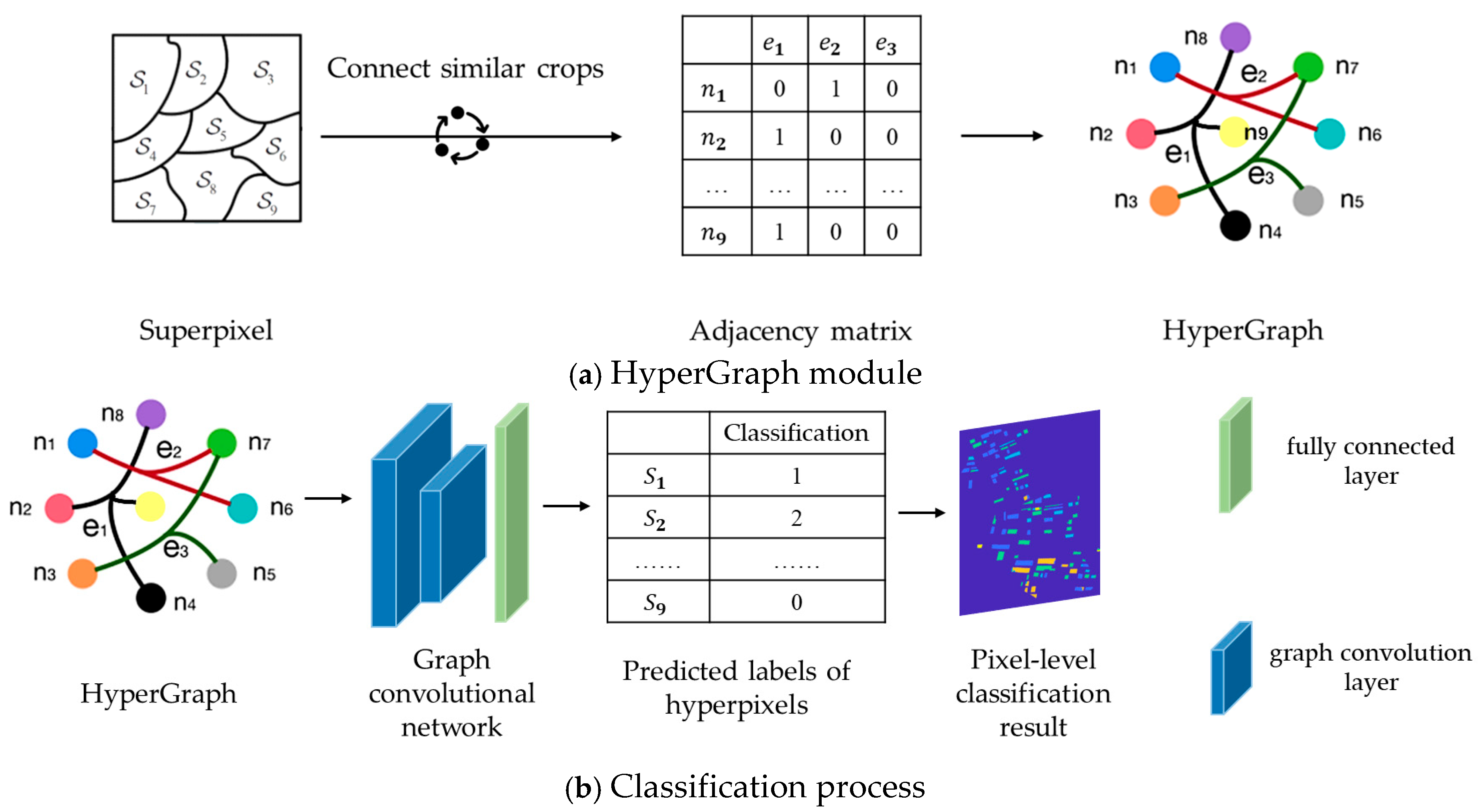
(2) A HyperGraph neural network was used to connect far-distant crop plots with others of the same type. Considering that although the same crop plots may be spatially dispersed, their scattering characteristics have certain similarities and correlations, this article utilized a HyperGraph neural network to establish higher-order relationships among multiple superpixels to effectively capture potential feature correlations and category consistency, so as to improve the accuracy and robustness of PolSAR data in crop classification.

(3) Different scattering features were extracted and combined to explore their classification performances in complex scenes. Four typical dual polarimetric features of superpixels, $\overline{H}$, $\overline{A}$, $\overline{alpha}$ and $\overline{{\lambda }_1}$, were extracted, and the classification was verified for each scattering feature one by one to explore its feasibility for crop classification. The classification accuracy was further investigated by feature combination; the classification of feature combination $\overline{H}+\overline{A}+\overline{{\lambda }_1}$ achieved the optimal accuracy on the experimental dataset.

2. Materials and Methods

2.1. Study Area

The experimental study area selected is the Flevoland region in the Netherlands. In order to avoid the influence of the observation alignment errors of different sensors on the observation results [28], the SLC data in the IW mode of Sentinel-1A are used in this article. In this study, the multi-temporal dataset of this region was downloaded through the Sentinel-1 open access platform. The real terrain classes were labeled according to the map provided by Khabbazan et al. [29] and Google Earth historical images.

The Flevoland time-series dataset was collected from May to August 2017, with a total of 8 scenes of data. The scene pixel size of the images is 637 × 644, and the real crop information and pseudo-color images are shown in Figure 1 and Figure 2. The dataset covers five crop types: potato, sugar beet, winter wheat, corn, and grass.

2.2. Related Works

2.2.1. Dual PolSAR Data Representation

The dual polarimetric SAR data can acquire the scattering information of the object in different combinations of electromagnetic wave transmission and reception polarimetric modes [30], and the polarimetric covariance matrix can analyze and interpret this information to reveal the polarimetric scattering features of the object. In the typical dual polarization VV/VH mode, the polarimetric covariance matrix is expressed as

$$C_2=\left[\begin{array}{cc}{S}_{vv}{S}_{vv}^{*}& S_{vv}{S}_{vh}^{*}\\ S_{vh}{S}_{vv}^{*}& S_{vh}{S}_{vh}^{*}\end{array}\right]$$

(1)

where $S_{vv}$ and $S_{vh}$ represent the scattering coefficients of vertical emission vertical reception and vertical emission horizontal reception, respectively. $*$ denotes the covariance transpose.

Other dual polarimetric data modes are similar to the VV/VH mode. Considering the main acquisition method of the Sentinel-1 TOPS mode, a detailed description of the VV/VH mode is provided.

The eigenvalue decomposition of the covariance matrix $C_2$ is expressed as Equation (2).

$$C_2=U\Lambda U^{-1}$$

(2)

where $\Lambda$ is the $2\times 2$ diagonal eigenvalue matrix; $\Lambda =diag({\lambda }_1,{\lambda }_2)$, which satisfies ${\lambda }_1\ge {\lambda }_2\ge 0$. ${\lambda }_1$ reflects the main scattering mechanism of the object. $U=[u_1,u_2]$ is the corresponding orthogonal eigenvector matrix, and each eigenvector satisfies the unit-module normalization. Based on the eigenvalue decomposition of the covariance matrix, three polarization features can be obtained.

The scattering entropy ($H$) describes the randomness of the object scattering, which takes the value in the range from 0 to 1, defined as

$$H={\displaystyle \sum _{i=1}^2-P_i{\log }_2}{P}_i\dots P_i={\displaystyle \frac{{\lambda }_i}{{\lambda }_1+{\lambda }_2}}$$

(3)

Complementing the scattering entropy parameter, the polarization anisotropy ($A$) describes the relative importance between two eigenvalues and is defined as

$$A=\left|{\displaystyle \frac{{\lambda }_1-{\lambda }_2}{{\lambda }_1+{\lambda }_2}}\right|$$

(4)

$A$ also ranges from 0 to 1. When the scattering intensities of the two scattering mechanisms are similar, $A$ is close to 0, indicating a more homogeneous scattering characteristic in the observation area. When the difference between the two eigenvalues is large, the $A$ increases, indicating that a certain scattering mechanism dominates the observation area.

The mean scattering angle ($alpha$) is closely related to the scattering mechanism, which ranges from 0° to 45°.

$$\alpha ={\displaystyle \sum _{i=1}^2{P}_i{\arccos }^{-1}\left(\left|u_i\right|\right)}$$

(5)

2.2.2. Dual PolSAR Wishart Distribution Characteristics

Multi-look processing of dual polarimetric SAR data is usually required, so as to reduce speckle, compress data and improve data quality. This process is realized by averaging several independent 1-look polarimetric covariance matrices [31]. Equation (6) defines the average covariance matrix after n-look processing.

$$C_2={\displaystyle \frac{1}{n}}{\displaystyle \sum _{k=1}^{n}u(k)u{(k)}^{*T}}$$

(6)

where $n$ denotes the number of looks and the vector $u(k)$ denotes the kth 1-look data sample.

The polarimetric covariance matrix after n-look processing can be expressed as Equation (7).

$$A=n{C}_2={\displaystyle \sum _{k=1}^{n}u(k)u{(k)}^{*T}}$$

(7)

It has been shown [32] that for multi-look polarimetric SAR data, the matrix obeys the complex Wishart distribution.

$$p^{(n)}(A)={\displaystyle \frac{L^{pn}{\left|A\right|}^{n-p}\exp \{-nTr({\sum }^{-1}A)\}}{R(n,p){\left|\sum \right|}^L}}$$

(8)

$$R(n,p)={\pi }^{{\displaystyle \frac{1}{2}}p(p-1)}\Gamma (n)\dots \Gamma (n-p+1)$$

(9)

where $\Sigma$ is the spatial ensemble average of the multi-look polarimetric covariance matrix. $\mathrm{Tr}({\Sigma }^{-1}\mathrm{A})$ denotes the trace of ${\Sigma }^{-1}\mathrm{A}$. $p$ denotes the dimension of the vector $u(k)$. $R(n,p)$ is the normalization factor. For dual polarization data, $p=2$. $\Gamma (•)$ is the gamma function, which is defined as

$${\Gamma }_p(n)={\pi }^{{\displaystyle \frac{p(p-1)}{2}}}{\displaystyle \prod _{i=0}^{p-1}\Gamma (n-i)}$$

(10)

Replacing $\Sigma$ with ${\sum }_{\mathrm{m}}$ as the covariance matrix of the class, rewrite $p^{(n)}(A)$ as $p(C_2|w_m)$, $C_2=A/n$. The maximum likelihood classifier will evaluate whether $C$ belongs to $w_{\mathrm{m}}$. Lee et al. [31] derived a distance measure by maximizing $p(C_2|w_m)$ for $P(w_m)$, defining the distance metric formula for classification of $n$-look polarimetric SAR data as

$$d(C_2,w_m)=n\ln \left|{\Sigma }_m\right|+n\mathrm{Tr}({\Sigma }_m^{-1}{C}_2)-\ln \left[P(w_m)\right]$$

(11)

As the number of looks, $n$, increases, the influence of the a priori probability $P(w_m)$ on category differentiation becomes smaller. In polarimetric SAR data, if nothing is known about the a priori probability of each category, it can be assumed that the a priori probability of different categories is the same, in which case the distance metric is independent of $n$. Equation (11) can be simplified as

$$d(C_2,w_m)=\ln \left|{\Sigma }_m\right|+\mathrm{Tr}({\Sigma }_m^{-1}{C}_2)$$

(12)

Equation (12) is the Wishart distance metric. In practice, due to the obvious differences in the scattering characteristics of crop categories in polarimetric SAR data, the Wishart model is able to capture these differences more accurately by modeling the polarimetric covariance matrix, thus achieving a finer distinction between crop types.

2.2.3. SLIC Superpixel Segmentation

Simple Linear Iterative Clustering (SLIC) is an efficient and widely used algorithm for superpixel segmentation, the core idea of which is to perform joint clustering of colors and spatial locations of pixel points in three-channel pseudo-color images of polarimetric data. It employs a weighted distance metric to balance the effects between color and spatial features, thus ensuring the uniformity of the superpixel regions and the integrity of the boundaries. The SLIC algorithm consists of the following main steps [33]:

(1) Initialize seed points: firstly, the image is divided into roughly equal $K$ grid regions based on the desired number of superpixels $K$, and a pixel from the center of each grid is selected as the initial seed point. The position of each seed point is $(x_i,y_i)$, and its color information is usually represented as the value $(l_i,a_i,b_i)$ in the CIELAB color space.

(2) Define the search range: the search range of each seed point is limited to a $2s\times 2s$ square area; $S$ is the spacing between the seed points; $s=\sqrt{N/K}$. $N$ denotes the total number of pixels in the image.

(3) Compute the distance metric: for each pixel, calculate its distance from nearby seed points. SLIC uses a united metric that combines color distance $d_{\mathrm{c}}$ and spatial distance $d_s$:

$$D={\displaystyle \frac{d_c}{m}}+{\displaystyle \frac{d_s}{s}}$$

(13)

$$d_c=\sqrt{{\left(l-l_i\right)}^2+{(a-a_i)}^2+{(b-b_i)}^2}$$

(14)

$$d_s=\sqrt{{\left(x_i-x_j\right)}^2+{(y_i-y_j)}^2}$$

(15)

(4) Assign pixels to the nearest seed point: based on the computed distance $D$, each pixel is assigned to the region of the superpixel to which the nearest seed point belongs; this process ensures that pixels with similar color and spatial features are classified into the same superpixel.

(5) Update the seed point position: for each superpixel region, the feature average of all pixels within its superpixel in color and spatial dimensions is computed and the seed point is moved to center-of-mass position, thus improving the representativeness of the seed point.

(6) Iterate optimization: repeat step (3) to step (5) until the seed point position no longer changes obviously, or the preset maximum number of iterations is reached. It has been shown [34] that the algorithm can converge after 10 iterations or less, so the number of iterations is often set to 10.

(7) Post-processing: each superpixel region is checked for connectivity, and disconnected small regions are subsumed into their neighboring superpixels, eliminating small isolated regions that may occur.

2.3. Proposed Method

2.3.1. SLIC Superpixel Segmentation Based on Multi-Temporal Dual Polarimetric Covariance Matrix

In order to solve the problem of superpixel inconsistency in temporal data due to color variations, this paper proposed an innovative approach that unites multi-temporal data for an integrated segmentation. In this method, the dual polarimetric covariance matrix of each temporal datum is formed into a block diagonal matrix, and this structure not only represents the polarimetric feature structure of different temporals, but also ensures that these features can be considered as a whole during the segmentation process, thus improving the accuracy and consistency of the segmentation across the growth period.

Suppose $C_2^t$ is a dual polarimetric covariance matrix for several temporals that follows a Wishart distribution $C_2^t~W(Df,\sum )$, $Df$ is the degree of freedom, and $\sum$ is covariance. Assuming that $C_2^t$ is independent, there is no correlation between each $C_2^t$. So $C$, as the block diagonal matrix, can be described as follows:

$$\begin{array}{l}C=\left[\begin{array}{ccccc}{C}_2^1& 0& 0& \dots & 0\\ 0& C_2^2& 0& \dots & 0\\ 0& 0& \ddots & \ddots & \dots \\ ⋮& ⋮& \ddots & \ddots & 0\\ 0& 0& \dots & 0& C_2^t\end{array}\right]\\ =\left[\begin{array}{ccccc}\left[\begin{array}{cc}{C}_{11}^1& {\mathrm{C}}_{12}^1\\ C_{21}^1& C_{22}^1\end{array}\right]& 0& 0& \dots & 0\\ 0& \left[\begin{array}{cc}{C}_{11}^2& {\mathrm{C}}_{12}^2\\ C_{21}^2& C_{22}^2\end{array}\right]& 0& \dots & 0\\ 0& 0& \ddots & \ddots & \dots \\ ⋮& ⋮& \ddots & \ddots & 0\\ 0& 0& \dots & 0& \left[\begin{array}{cc}{C}_{11}^t& {\mathrm{C}}_{12}^t\\ C_{21}^t& C_{22}^t\end{array}\right]\end{array}\right]\end{array}$$

(16)

The $C_2^t$ for each temporal is jointly constructed into the block diagonal covariance matrix in Equation (16).

For each $C_2^t$, this can be expressed as

$$C_2^t={\mathrm{x}}_t\cdot {\mathrm{x}}_t^{*T}$$

(17)

Then

$$\begin{array}{l}C=\left[\begin{array}{ccccc}{x}_1\cdot x_1^{*T}& 0& 0& \dots & 0\\ 0& x_2\cdot x_2^{*T}& 0& \dots & 0\\ 0& 0& \ddots & \ddots & \dots \\ ⋮& ⋮& \ddots & \ddots & 0\\ 0& 0& \dots & 0& x_t\cdot x_t^{*T}\end{array}\right]\\ =\left[\begin{array}{ccccc}{x}_1& 0& 0& \dots & 0\\ 0& x_2& 0& \dots & 0\\ 0& 0& \ddots & \ddots & \dots \\ ⋮& ⋮& \ddots & \ddots & 0\\ 0& 0& \dots & 0& x_t\end{array}\right]\cdot {\left[\begin{array}{ccccc}{x}_1& 0& 0& \dots & 0\\ 0& x_2& 0& \dots & 0\\ 0& 0& \ddots & \ddots & \dots \\ ⋮& ⋮& \ddots & \ddots & 0\\ 0& 0& \dots & 0& x_t\end{array}\right]}^{*T}\\ =X\cdot X^{*T}\end{array}$$

(18)

Wishart distribution has independent additivity. In the construction of the block diagonal matrix $C$, the generation of each submatrix $C_2^t$ satisfies the above conditions and they are independent of each other. Therefore, the block diagonal matrix $C$ constructed from these submatrices also satisfies the generation of the Wishart distribution, and the covariance structure of the block diagonal matrix $C$ still maintains the block diagonal shape.

$$\Sigma =\left[\begin{array}{ccccc}{\Sigma }_1& 0& 0& \dots & 0\\ 0& {\Sigma }_2& 0& \dots & 0\\ 0& 0& \ddots & \ddots & \dots \\ ⋮& ⋮& \ddots & \ddots & 0\\ 0& 0& \dots & 0& {\Sigma }_t\end{array}\right]$$

(19)

The probability density function of the block diagonal matrix $C$ is shown in Equation (20).

$$f(C)={\displaystyle \prod _{t=1}^{a}f(C_2^t)}$$

(20)

where $f(C_2^t)$ is the probability density function of each sub-block. This study replaces the color distance formula $d_{\mathrm{c}}$ in the SLIC method with the Wishart distance formula $d_w$. For each sub-block, $C_2^t$ can calculate its Wishart distance.

$$d(i,j)=\ln \left(\left|{\Sigma }_j\right|\right)+Tr({\Sigma }_j^{-1}{C}_2^t)$$

(21)

Then the Wishart distance of the block diagonal matrix $C$ is the sum of the Wishart distances of the sub-blocks $C_2^t$.

$$d_w(i,j)={\displaystyle \sum _{n=1}^t(\ln \left(\left|{\Sigma }_j\right|\right)+Tr({\Sigma }_j^{-1}{C}_2^t)})$$

(22)

where $i$ denotes each pixel point, $j$ denotes each superpixel, and ${\sum }_j$ denotes the covariance matrix at the center of each superpixel.

The new SLIC superpixel segmentation Equation (23) is finally obtained instead of Equation (13).

$$D={\displaystyle \frac{d_w}{m}}+{\displaystyle \frac{d_s}{s}}$$

(23)

2.3.2. Extraction of Superpixel Polarimetric Features

The superpixel segmentation method based on the temporal dual polarimetric covariance matrix divided the data into several superpixel regions, and each superpixel region is partitioned by spatial distance with a Wishart distance matrix. It is assumed that the result after superpixel segmentation can be represented as a set $\left\{S_1,S_2,\dots ,S_n\right\}$ of superpixel regions, where each $S_i$ represents a superpixel region, and it satisfies that the union of all superpixels is the entire image region $I$.

$$I={\displaystyle \underset{i=1}{\overset{n}{\cup }}{S}_i}$$

(24)

For PolSAR data, scattering features are the main form of expression, which contains rich distinctive information. After the superpixel segmentation was completed, this section utilized each superpixel region as a mask to localize the features in order to fully explore the unique information within each superpixel region.

Suppose a superpixel region $S_i$ contains a collection of pixels as $\left\{p_1,p_2,\dots ,p_m\right\}$, for a scattering feature matrix $M$, where each pixel point $p_i$ contains a scattering feature $m(p_i)$. By applying a masking operation to the superpixel region $S_i$, it is possible to extract the features of all the pixels from this region, forming the masked set of features $M(S_i)$.

$$M(S_i)=\left\{m(p_1),m(p_2),m(p_3),\dots ,m(p_m)\right\}$$

(25)

For the features within each superpixel region, the statistics were calculated. Since the superpixel segmentation not only takes into account the similarity between pixels, but also takes into account the changing features of the time series data, thus ensuring the consistency of the categories within each superpixel region to a large extent. Based on this, the mean value of the features within the region was calculated in order to obtain the representative features within the region. The mean value of the features in a superpixel region $S_i$ can be expressed as

$${\mu }_{S_i}={\displaystyle \frac{1}{m}}{\displaystyle \sum _{p\in S_i}m(p)}$$

(26)

By statistically quantifying the features of all the superpixel regions, a new feature can be obtained in which each superpixel region has a mean value representing its local features. These means were effective in reflecting the characteristics of dual polarization in the region, and $\overline{H}$, $\overline{A}$, $\overline{alpha}$ and $\overline{{\lambda }_1}$ were extracted for this study. The feature can be used in subsequent classification tasks to help the classification model better capture changes in crop type and growth state.

2.3.3. Establishing Spatial Distribution Relationship with HyperGraph Neural Network

In crop classification, crop plots often exhibit spatial dispersion, that is, the same crop is not necessarily planted continuously, which poses a challenge to the classification task. For such dispersed plots, the HyperGraph is able to consider them comprehensively from the local superpixel scale to the larger farm scale. At the local scale, the HyperGraph can focus on the features inside each superpixel to capture the detailed information; while at the farm scale, through the connection of hyperedges, the HyperGraph can effectively combine the scattered superpixels into a larger region, so as to grasp the distribution pattern of the same crop plots, and then realize the effective classification of these scattered plots. The nodes of the HyperGraph can represent the features of a single plot, while the hyperedges of it help establish the recognition of different plots by connecting multiple plots with similar features. Regardless of whether these parcels are spatially neighboring or not, as long as they possess similarity in certain features, they can be connected by a hyperedge. The nodes and hyperedges of the HyperGraph enhance its ability to handle tasks with complex similarity relationships, especially in crop classification, to effectively recognize plots of the same category with different distances.

The core of the HGNN lies in the construction of the HyperGraph, which can connect multiple nodes and learn the features of all nodes on the same hyperedge, and thus the higher-order associations between objects. In this study, a HyperGraph was constructed based on ground-truth labels of the training superpixels. This means that each crop type has a distinct hyperedge, effectively grouping known classes regardless of their spatial locations. The HGNN then utilizes this structure to learn features on the hyperedges. The entire process is detailed in Algorithm 1. A HyperGraph $\mathcal{H}$ is a binary group $\mathcal{H}=(V,E)$, where $V=\{v_1,v_2,\dots ,v_n\}$ denotes set of nodes, containing $n$ nodes, and $E=\{{\mathrm{e}}_1,{\mathrm{e}}_1,\dots ,{\mathrm{e}}_m\}$ denotes the set of hyperedges. Each hyperedge can connect multiple nodes.

Algorithm 1. HyperGraph Construction

Input: $L$: set of node labels, $L=\{l_1,l_2,l_3,\dots ,l_n\}$ $V$: set of nodes, $\left|V\right|=N$ $F$: feature matrix for nodes

Output: $H$: adjacency matrix of the HyperGraph

Steps:

1: Initialize HyperGraph $\mathcal{H}=(V,E)$

2: Extract unique labels $U=\{u_1,u_2,\dots ,u_{\mathrm{m}}\}$ from $L$

3: For each unique label $u_j\in U$ where $j\in \left[1,m\right]$:

Find node indices $S_j=\left\{i\right|L\left[i\right]=u_j,i\in \left[1,N\right]\}$

Add hyperedge $e_j=S_j$ to $E$, $E=E\cup \left\{e_j\right\}$

4: Construct adjacency matrix $H$ where $i\in S_j$:

Set $H[i,j]=1$

Given a HyperGraph $\mathcal{H}$, its structure can be represented by an adjacency matrix $H\in {ℝ}^{n\times m}$.

$$H(v_i,e_{\mathrm{j}})=\left\{\begin{array}{c}1,\\ 0,\end{array}\right.\begin{array}{c}\\ \end{array}\begin{array}{c}\\ \end{array}\begin{array}{c}\mathit{if}{v}_i\in e_{\mathrm{j}}\\ \mathit{if}{v}_i\notin e_{\mathrm{j}}\end{array}$$

(27)

where $H(v_i,e_{\mathrm{j}})$ denotes whether node $v_{\mathrm{i}}$ belongs to a hyperedge $e_j$. If $h(v_i,e_{\mathrm{j}})=1$, $v_{\mathrm{i}}$ belongs to $e_j$, otherwise $h(v_i,e_{\mathrm{j}})=0$. The degree $D(v_{\mathrm{i}})$ of each node in the HyperGraph denotes the number of hyperedges connected to that node, defined as

$$D(v_i)={\displaystyle \sum _{e_j\in E}h(}{v}_i,e_j)$$

(28)

And the degree $D(e_j)$ of a hyperedge denotes the number of nodes contained in that hyperedge, defined as

$$D(e_j)={\displaystyle \sum _{v_i\in V}h(}{v}_i,e_j)$$

(29)

In the HGNN, the HyperGraph structure is mainly utilized and combined with multiple graph convolutional layers and fully connected layers. The purpose of these structures is to achieve feature aggregation, propagation and classification. The process of feature aggregation and propagation is carried out through hyperedges, the structure is shown in Figure 3a. Each node receives information from other nodes through the hyperedges, similar to the “message passing mechanism” in a traditional graph neural network (GNN). However, unlike a GNN, an HGNN can receive information from multiple related nodes through the hyperedge at the same time, and learn the features of each node on the hyperedge, which makes it possible to learn richer feature expressions in the classification task. The classification process based on HGNN is shown in Figure 3b.

The content and form of each network layer of the HGNN is as follows. The input layer receives the feature of the node.

$$X\in R^{N\times d}$$

(30)

where $N$ is the number of nodes and $d$ is the feature dimension of each node. In this study, the input features are superpixel scattering features.

The main task of the first graph convolution layer is to update the feature representation of each node by aggregating the information of neighboring nodes through hyperedges. This process mainly relies on the adjacency matrix $H$ and the features of node $X$ to realize. Firstly, the connection relationships between nodes in the adjacency matrix $H$ are used to clarify which nodes belong to the same hyperedge. Then, based on these connection relationships, the information of nodes is aggregated. The features of nodes are updated as Equation (31), and the adjacency matrix is updated as Equation (32).

$$X^{(1)}=\sigma (H’X{W}^{(1)})$$

(31)

$$H’=D_v^{-{\displaystyle \frac{1}{2}}}H{W}_e{D}_e^{-1}{H}^{\mathrm{T}}{D}_v^{-{\displaystyle \frac{1}{2}}}$$

(32)

where $W^{(1)}$ is the learnable weight matrix of the first layer, and the network automatically adjusts these weights during the training process to learn the most effective feature representation; $\sigma$ is the nonlinear activation function, and the ReLU function is used to introduce nonlinear factors to enhance the expressive ability of the network; $D_v$ and $D_e$ are the node degree matrix and the hyperedge degree matrix, respectively, which are used to normalize the correlation matrix and to ensure the information aggregation stability.

The second graph convolutional layer is similar to the first one, and again the updated features are aggregated by hyperedges. The process of feature updating is as follows:

$$X^{(2)}=\sigma (H’X^{(1)}{W}^{(2)})$$

(33)

where $W^{(2)}$ is the learnable weight matrix of the second layer, again continuously adjusted during training to further extract more discriminative features.

After feature extraction by the two graph convolution layers, the resulting feature $X^{(2)}$ is fed to the fully connected layer for final classification. The fully connected layer maps the extracted features to the category space as in Equation (34).

$$Y=\mathrm{softmax}(X^{(2)}{W}^{(3)}+b)$$

(34)

where $W^{(3)}$ is the weight matrix of the fully connected layer, $b$ is the bias term, and $Y$ is the output after a softmax activation function indicating the predicted probability of each category.

By constructing the HGNN and performing multi-layer message passing, the HyperGraph is able to capture the higher-order relationships between plots and gradually learn the complex relationships between nodes through multi-layer convolution. This multi-layer message propagation mechanism enables the HyperGraph to better handle spatial dispersion and complex plot characteristics in crop classification.

2.4. Overall Process

Figure 4 gives the overall flowchart of this article’s method. The proposed method consists of two main steps: superpixel segmentation based on multi-temporal polarimetric covariance matrices and classification for establishing spatial distribution relations using a HyperGraph neural network.

In the first step, the diagonal polarimetric covariance matrix is constructed by uniting a dual polarimetric covariance matrix of each temporal data. Then, considering that the dual polarimetric covariance matrix obeys the Wishart distribution characteristic, the traditional SLIC segmentation formula is modified for the multi-temporal data to obtain the superpixel segmentation results that are more stable, and then scattering features of each multi-temporal superpixel are extracted.

In the second step, a HyperGraph neural network is used to classify the obtained multi-temporal superpixel in the previous step. Compared with a traditional neural network, an HGNN is able to better deal with complex unstructured data, and it can effectively capture the complex relationship between the superpixels, and make full use of the multi-dimensional information of time–polarization–space to classify the superpixels. In order to apply the classification results to a real scene, the predicted labels of these superpixels are finally reconstructed back to the pixel level to obtain the final classification results.

3. Results and Discussion

3.1. Experimental Settings

To ensure the accuracy of the training data, about 6% of the labeled superpixels of the total superpixel data volume are selected from the segmentation results, and these superpixels are used to construct the adjacency matrix, and as the model training set. In the testing step, all the superpixels are used for the test in order to comprehensively assess the performance of the model. In the HyperGraph classification model, the Adam optimizer is used to train 200 epochs at a learning rate of 0.01.

To achieve a more intuitive and accurate presentation of the classification results, the pixel location information contained in each superpixel is recorded during the process of segmentation. After the HGNN completes the task of classifying, the predicted category labels of each superpixel are converted back to pixel labels. Through this reverse conversion process, the classification results at the superpixel level can be refined to the pixel level, thus obtaining the final, higher-resolution classification results.

3.2. Experimental Results

In this article, the method is validated and discussed through experiments in three aspects: (1) Firstly, in the step of superpixel segmentation, the effects of different parameters on the superpixel segmentation results are analyzed. At the same time, in order to show the advantages of multi-temporal information in superpixel segmentation, the effects of single-temporal and multi-temporal superpixel segmentation are compared. (2) Secondly, in the research of superpixel classification features, the classification effects of different polarimetric features for dual polarimetric data under the HGNN are compared, as well as the possible feature combinations, to examine the influence of input features and, further, to obtain the optimal feature combinations. (3) Finally, in terms of classification model performance evaluation, the performance of the HGNN, GNN, and RF are compared in the superpixel classification task, in order to validate the advantages of combining superpixels and the HyperGraph in crop classification.

3.2.1. Analysis of Superpixel Segmentation Results

➢

Effect of seed points on superpixel segmentation

As a key step, the setting of different seed points can obviously change the effect of superpixel segmentation. This section describes experiments conducted for different seed points. The seed point directly affects the step length of superpixel segmentation; it has an inverse relationship with the step length. The step length determines the size and density of the superpixels, with a smaller step length typically generating more pairs of smaller-sized and finer superpixels, while a larger step length generates fewer but larger superpixels. This tuning helps to balance the computational complexity of segmentation with accuracy.

In the experiments, the number of seed points was set to 1000, 1500, 2000, 2500, 3000 and 3500, and the superpixel segmentation edges with different seed points are shown in Figure 5. It was found that when the number of seed points is 2500, the generated superpixels are of moderate number and reasonable size, which can effectively capture the boundary of the parcel in the image, avoiding the problem of excessive refinement or too much roughness.

In contrast, when the numbers of seed points were 1000, 1500 and 2000, the segmentation results appeared too coarse to accurately distinguish the boundaries of different parcels due to the large step length. Especially when the number of seed points was 1000, the generated superpixel area was too large, resulting in the neighboring regions being unable to be effectively distinguished, and the superpixel merged several different plots into one large parcel. When the numbers of seed points were 3000 and 3500, the step length was smaller, and although the superpixels became more detailed, the over-refined superpixels not only increased the computational complexity and prolonged the processing time, but also made the segmentation results too redundant, which affected the efficiency of the subsequent processing.

Combining the above experimental results and analysis, the 2500 seed point number is considered optimal for this experiment, which provides a good balance between segmentation accuracy and computational complexity.

➢

Comparative analysis of single-temporal with multi-temporal superpixel segmentation

The experiment further compared the effect of single-temporal with multi-temporal superpixel segmentation to verify the effect of temporal information on the superpixel segmentation results.

For single-temporal superpixel segmentation, the same SLIC method was used for superpixel generation by replacing the color distance with the Wishart distance. The single-temporal superpixel segmentation algorithm acted independently on the data of each temporal to ensure that the segmentation processes did not interfere with each other. To ensure the comparability of the experiments, the experimental process kept the number of seed points at 2500, and the results are shown in Figure 6. Observing the results presented in Figure 6a–c, it can be seen that there were obvious differences in the size and shape of the region obtained from the segmentation of each temporal, and different types of plots are not effectively distinguished in the segmentation image.

Simultaneously, for comparison, we also performed superpixel segmentation on single-time data using the traditional SLIC algorithm based on RGB distance under the same parameter setting of 2500 seed points. As shown in Figure 7, the traditional SLIC method was unable to distinguish between different crop regions.

Obviously different from single-temporal segmentation, multi-temporal superpixel segmentation exhibited better results, as shown in Figure 5d and Figure 6d. The algorithm was able to identify the features that change over time, which enabled the parcels that behave similarly at different time points to be classified into the same superpixel region, improving the consistency and accuracy of segmentation. Multi-temporal segmentation not only takes into account spatial information, but it is also able to capture subtle changes due to temporal variations.

During the crop growth cycle, the differences in the plots at different stages in SAR images may be subtle, and are difficult to accurately distinguish by traditional single-time segmentation methods. In contrast, temporal union segmentation can clearly distinguish these subtle changes and use them as the basis for superpixel division by comprehensively analyzing multi-temporal data, so that crop plots at different growth stages can be more accurately divided.

3.2.2. Classification Results of HGNN

The extracted scattering features for each superpixel were input into the HGNN. Based on the information of the superpixels, the network set a hyperedge for each category and grouped all similar superpixels into one group, and the node–hyperedge adjacency matrix could be constructed using the set of hyperedges.

In order to verify the effectiveness of the object-oriented HGNN, four types of scattering features obtained at different seed points were selected for comparison experiments in this study.

The classification accuracies of the four superpixel scattering features in the HGNN network of this experiment are shown in

Table 1. Classification accuracy of HGNN under different superpixel setting conditions.

Seed Point	Superpixel Scattering Feature	Overall Accuracy (OA)
1000	$\overline{H}$	80.93%
	$\overline{A}$	80.01%
	$\overline{alpha}$	79.63%
	$\overline{{\lambda }_1}$	86.60%
1500	$\overline{H}$	81.16%
	$\overline{A}$	85.03%
	$\overline{alpha}$	80.27%
	$\overline{{\lambda }_1}$	89.81%
2000	$\overline{H}$	83.69%
	$\overline{A}$	87.11%
	$\overline{alpha}$	82.97%
	$\overline{{\lambda }_1}$	90.27%
2500	$\overline{H}$	85.08%
	$\overline{A}$	90.15%
	$\overline{alpha}$	85.40%
	$\overline{{\lambda }_1}$	92.07%
3000	$\overline{H}$	85.88%
	$\overline{A}$	89.27%
	$\overline{alpha}$	85.66%
	$\overline{{\lambda }_1}$	91.86%
3500	$\overline{H}$	85.85%
	$\overline{A}$	89.67%
	$\overline{alpha}$	86.35%
	$\overline{{\lambda }_1}$	92.89%

. In general, the classification accuracy of each superpixel scattering feature shows a trend of first increasing and then leveling off with the increase in the number of seed points. Specifically, when the number of seed points was 1000, the classification accuracy of $\overline{H}$, $\overline{A}$ and $\overline{alpha}$ was relatively low, and the classification accuracy of $\overline{{\lambda }_1}$ was relatively high. When the number of seed points was increased to 2500, the classification accuracies of the four superpixel scattering features $\overline{H}$, $\overline{A}$, $\overline{alpha}$ and $\overline{{\lambda }_1}$ reached 85.08%, 90.15%, 85.40%, and 92.07%, respectively. When the number of seed points increased from 2500 to 3500, the improvement in classification accuracy was marginal, while the computational cost for superpixel segmentation rose significantly. Therefore, a setting of 2500 seed points effectively controls computational cost while ensuring high accuracy, achieving the best trade-off between precision and efficiency. Thus, in this experiment, it is considered that the overall classification effect reaches an optimal state with this setting. After this, the classification accuracy tended to stabilize by continuing to increase the number of seed points. By comparing the classification accuracies of these four scattering features, it can be found that $\overline{{\lambda }_1}$ shows better results than the other three under different seed points. When the seed point number was 2500, the classification effect corresponded to the effect of superpixel segmentation.

Next, the effectiveness of multi-temporal superpixel classification was verified, as shown in

Table 2. Comparison of single-temporal and multi-temporal superpixel classification results.

		Superpixel Scattering Feature	Overall Accuracy (OA)
Single- temporal Superpixel	19 May 2017	$\overline{H}$	64.83%
		$\overline{A}$	65.04%
		$\overline{alpha}$	60.59%
		$\overline{{\lambda }_1}$	51.71%
	31 May 2017	$\overline{H}$	57.33%
		$\overline{A}$	56.01%
		$\overline{alpha}$	53.80%
		$\overline{{\lambda }_1}$	57.93%
	12 June 2017	$\overline{H}$	60.34%
		$\overline{A}$	59.64%
		$\overline{alpha}$	55.46%
		$\overline{{\lambda }_1}$	63.89%
	24 June 2017	$\overline{H}$	67.48%
		$\overline{A}$	65.99%
		$\overline{alpha}$	60.10%
		$\overline{{\lambda }_1}$	63.10%
	6 July 2017	$\overline{H}$	61.67%
		$\overline{A}$	64.69%
		$\overline{alpha}$	55.72%
		$\overline{{\lambda }_1}$	65.28%
	18 July 2017	$\overline{H}$	58.11%
		$\overline{A}$	55.49%
		$\overline{alpha}$	51.19%
		$\overline{{\lambda }_1}$	65.14%
	30 July 2017	$\overline{H}$	61.56%
		$\overline{A}$	58.63%
		$\overline{alpha}$	60.32%
		$\overline{{\lambda }_1}$	65.13%
	11 August 2017	$\overline{H}$	50.24%
		$\overline{A}$	41.74%
		$\overline{alpha}$	43.01%
		$\overline{{\lambda }_1}$	64.90%
Multi-temporal Superpixel	8 temporal data	$\overline{H}$	85.08%
		$\overline{A}$	90.15%
		$\overline{alpha}$	85.40%
		$\overline{{\lambda }_1}$	92.07%

. This indicated that integrating data from multi-temporal data can effectively overcome the limitations of single-time data. By using complementary information along the temporal dimension, this approach reduced random errors and the influence of environmental factors, enabling a more comprehensive characterization of crop changes, and led to a substantial improvement in classification accuracy.

On the basis of single-feature classification, we further developed multi-feature combination classification under the condition of the optimal parameter of 2500 seed points, which has been verified by previous experiments.

Table 3. Classification results of HGNN with different superpixel scattering feature combinations.

Feature Combination	Overall Accuracy (OA)	Average Accuracy (AA)	Kappa
$\overline{H}+\overline{A}$	92.72%	78.50%	0.8988
$\overline{H}+\overline{alpha}$	86.72%	75.55%	0.8158
$\overline{A}+\overline{alpha}$	92.33%	83.06%	0.8942
$\overline{H}+\overline{{\lambda }_1}$	94.20%	84.91%	0.9197
$\overline{A}+\overline{{\lambda }_1}$	95.01%	85.16%	0.9309
$\overline{alpha}+\overline{{\lambda }_1}$	90.61%	83.76%	0.8704
$\overline{H}+\overline{A}+\overline{alpha}$	93.40%	82.67%	0.9088
$\overline{H}+\overline{A}+\overline{{\lambda }_1}$	95.74%	88.93%	0.9412
$\overline{A}+\overline{alpha}+\overline{{\lambda }_1}$	93.49%	83.88%	0.9102
$\overline{H}+\overline{alpha}+\overline{{\lambda }_1}$	91.31%	82.45%	0.8799
$\overline{H}+\overline{A}+\overline{alpha}+\overline{{\lambda }_1}$	94.18%	87.87%	0.9197

compares the overall classification performance of different superpixel feature combinations. The experimental results show that the classification effect of the feature combination with $\overline{{\lambda }_1}$ is improved. The classification accuracy of $\overline{H}+\overline{A}+\overline{{\lambda }_1}$ is 95.74%, and its classification result is shown in Figure 8b. It is worth mentioning that when the feature combination is $\overline{H}+\overline{A}+\overline{alpha}+\overline{{\lambda }_1}$, its classification accuracy is not as high as that of the $\overline{H}+\overline{A}+\overline{{\lambda }_1}$. This performance degradation is likely because $\overline{alpha}$ does not contribute new and valuable scattering information. As shown in Table 1, the classification performance of $\overline{alpha}$ alone is poor. The scattering mechanism information provided by $\overline{alpha}$ lacks sufficient discriminative power for the crop types in this study. During the growth stages, the scattering mechanism for most of these crops is predominantly volume scattering. Consequently, their $\overline{alpha}$ values are concentrated within a range of approximately 45° to 90°, which cannot provide the distinctive information needed to differentiate among these categories.

To further evaluate the model’s classification performance under the optimal parameter settings, 2500 seed points and the $\overline{H}+\overline{A}+\overline{{\lambda }_1}$ feature combination, we analyze the classification accuracy for each crop class in detail.

Table 4. Confusion matrix for the classification using the $\overline{H}+\overline{A}+\overline{{\lambda }_1}$ feature combination.

	Wheat	Sugar Beet	Potato	Grass	Maize
Wheat	11953	36	1	83	0
Sugar Beet	8	4370	627	3	0
Potato	0	37	9782	0	0
Grass	74	54	0	4646	0
Maize	37	71	373	0	767

presents the classification confusion matrix, while

Table 5. PA and UA for each crop using the $\overline{H}+\overline{A}+\overline{{\lambda }_1}$ feature combination.

	PA	UA
Wheat	0.9901	0.9901
Sugar Beet	0.9567	0.8726
Potato	0.9072	0.9962
Grass	0.9818	0.9732
Maize	1.0000	0.6146

lists the Producer’s Accuracy (PA) and User’s Accuracy (UA) for each category.

The model demonstrates strong discriminative ability for wheat, beet, potato, and grass, but its classification performance for corn is comparatively poor. It is noteworthy that while the PA for corn reaches a perfect 1.0000, its UA is only 0.6146. Upon analysis, this discrepancy does not stem from issues in the model’s algorithmic design, architecture, or training optimization. Instead, it is attributed to the significantly low proportion of corn samples in the dataset. Out of a total of 32,922 labeled pixels in the entire dataset, only 1248 are labeled as corn, accounting for just 3.79%. After superpixel segmentation, the number of superpixels corresponding to corn becomes even smaller. This scarcity means that during the training phase, the model’s learning of corn features is concentrated on an extremely limited set of examples. It becomes highly proficient at identifying these few specific samples in the training set, leading to the high PA. However, in practical scenarios where sample distribution is more diverse and complex, the model lacks learning experience from a sufficient variety of corn samples. This makes it difficult to effectively distinguish other classes from corn, causing a large number of non-corn samples to be misclassified as corn. Consequently, the UA value is substantially lower.

3.2.3. Comparative Performance Analysis of HGNN and Other Classification Models

In order to evaluate the effectiveness of the HGNN, experiments were conducted to compare and analyze the classification performance of the other two typical classification models, namely, the random forest (RF) and the graph neural network (GNN), based on different scattering features. The relevant experiments were conducted with seed points of 2500 and the same superpixel features as the input. From the experimental results in

Table 6. Comparison of classification accuracy among the three classification models.

Classification Model	Superpixel Scattering Feature	Overall Accuracy (OA)
RF	$\overline{H}$	74.54%
	$\overline{A}$	74.73%
	$\overline{alpha}$	76.41%
	λ1	75.90%
	$\overline{H}+\overline{A}+\overline{{\lambda }_1}$	80.45%
GNN	$\overline{H}$	82.45%
	$\overline{A}$	86.54%
	$\overline{alpha}$	83.92%
	λ1	90.95%
	$\overline{H}+\overline{A}+\overline{{\lambda }_1}$	93.17%
HGNN	$\overline{H}$	85.08%
	$\overline{A}$	90.15%
	$\overline{alpha}$	85.40%
	λ1	91.59%
	$\overline{H}+\overline{A}+\overline{{\lambda }_1}$	95.74%

, it can be seen that the different models show obvious differences. The RF classifier has a lower accuracy compared to the other two models, with its classification accuracy only ranging from about 74.54% to 80.45%. This is due to its structure based on decision tree integration, which has some limitations in dealing with complex feature information, and it does not consider spatial relationships, making it difficult to fully explore the potential relationships in the data. The classification accuracy of the GNN model is obviously improved compared to the RF, with its classification accuracy ranging from 82.45% to 93.17%. This is due to its ability to effectively capture the graph structure information in the data and better utilize the correlation relationship between the data when dealing with features. The HGNN model performs better, with a classification accuracy ranging from 85% to 95.74%. As a more advanced model architecture, the HGNN has a unique advantage in dealing with higher-order relationships and complex structured data, and it can extract the key information of scattering features with greater accuracy, thus achieving higher accuracy and better performance.

3.3. Methodological Applicability, Limitations and Future Research

This method is suitable for dealing with complex crop classification with multi-temporal dual polarimetric SAR data, especially for solving the fine classification problem of crops with uneven spatial distribution, such as broken farmland and mixed planting areas. By improving SLIC superpixel segmentation through the united multi-temporal dual polarimetric covariance matrix, it can effectively resist the interference of temporal differences and capture the crop boundaries. Combined with the HGNN, when constructing the higher-order spatial correlation among the obtained superpixels, the classification accuracy of farmland parcels is obviously improved. However, its performance relies on high-quality and continuous temporal polarimetric SAR data.

In the future, the superpixel segmentation algorithm can be adaptively adjusted in real time according to the crop growth state, so that the segmentation process not only considers the spatial characteristics, but also dynamically combines the temporal changes and crop physiological parameters to realize on-demand and accurate segmentation.

4. Conclusions

To address the problem of insufficiently utilizing information about the comprehensive spatial distribution of crops near and far, a multi-temporal dual polarimetric SAR classification method based on superpixels and a HyperGraph is designed. Firstly, using the property that the polarimetric covariance matrix obeys the Wishart distribution, superpixel segmentation is performed on the multi-temporal dual PolSAR data, so that the shape and size of the superpixel segmentation of each temporal are consistent and in accordance with the actual plots. Secondly, the HyperGraph adjacency matrix is constructed based on superpixels, and then classified by the HGNN, which learns the features of the same crop across different plots, and effectively improves the accuracy of the classification.

The experimental results show that the HGNN effectively integrates the scattering features and spatial information of dual polarimetric SAR data through the multi-dimension data of time–polarization–space. Under the optimal parameter configuration, with 2500 seed points and the $\overline{H}+\overline{A}+\overline{{\lambda }_1}$ feature combination, the overall classification accuracy reaches 95.74%, which is improved compared with both the GNN and RF methods. The experiments verify the effectiveness of the dual polarimetric scattering feature extraction based on multi-temporal superpixels and the HGNN as the classification network. It also provides a new technical framework for crop classification in complex agricultural scenes.