Article

Remote Sensing and Critical Slowing Down Modeling Reveal Vegetation Resilience in the Three Gorges Reservoir Area, China

1
China Institute of Geo-Environment Monitoring, China Geological Survey, Beijing 100081, China
2
School of Geography and Planning, Chengdu University of Technology, Chengdu 610059, China
3
School of Earth Sciences and Engineering, Hohai University, Nanjing 210024, China
4
School of National Safety and Emergency Management, Beijing Normal University, Beijing 100875, China
5
Department of Geography, The University of Hong Kong, Hong Kong SAR 999077, China
*
Author to whom correspondence should be addressed.
The authors (Liangliang Zhang and Nan Yang) contributed equally to this work.
Remote Sens. 2025, 17(13), 2297; https://doi.org/10.3390/rs17132297
Submission received: 14 May 2025 / Revised: 20 June 2025 / Accepted: 26 June 2025 / Published: 4 July 2025

Abstract

Globally, ecosystems are affected by climate change, human activities, and natural disasters, which impact ecosystem quality and stability. Vegetation plays a crucial role in ecosystem material cycle and energy transformation, making it important to monitor its resilience under disturbance stress. The Critical Slowing Down (CSD) indicates that as ecosystems near collapse, the autocorrelation of lag temporal increases and resilience decreases. We used the lag Temporal Autocorrelation (TAC) of long-term remote sensing Leaf Area Index (LAI) to monitor vegetation resilience in the Three Gorges Reservoir Area (TGRA). The Disturbance Event Model (DEM) was used to validate the CSD. The results showed the following: (1) The eastern TGRA exhibited high and increasing vegetation resilience, while most areas showed a decline. (2) Among the various vegetation types, forests demonstrated higher resilience than other vegetation types. (3) Precipitation, temperature, and soil moisture significantly influenced vegetation resilience dynamics within the TGRA. (4) For model accuracy, the CSD’s results were consistent with the DEM, confirming its applicability in the TGRA. Overall, the CSD when applied to long-term remote sensing data, provided valuable quantitative indicators for vegetation resilience. Furthermore, more CSD-based indicators are needed to analyze vegetation resilience dynamics and better understand the biological processes determining vegetation degradation and restoration.

1. Introduction

When a complex ecosystem approaches the edge of a steady-state transition, it is characterized by a gradual loss of resilience [1,2,3]. Resilience refers to the ability to self-regulate and recover after deviating from an equilibrium state owing to external disturbances [4]. Recent work has found critical transitions when vegetation is exposed to serious natural disturbances (e.g., droughts and high temperatures) [5,6], and reduced resilience is an important driving factor for critical vegetation transition [7,8]. The Critical Slowing Down (CSD) theory states that the rate at which a system returns to equilibrium following an external disturbance can be determined from its internal natural fluctuations. The fluctuations in the state of a system can reflect slowing down through an increase in temporal autocorrelation (TAC). Temporal autocorrelation (TAC) refers to the correlation of a variable with itself at a prior time step. It quantifies the extent to which current system states depend on their past values. An increase in TAC indicates that the system is taking longer to recover from perturbations, which is a key signal of Critical Slowing Down (CSD). In addition, TAC is an indicator that can be calculated pixel by pixel using satellite grid data, suggesting that this is a new way to monitor vegetation resilience and other ecosystems prone to collapse.
On a global scale, research on vegetation resilience has revealed that humid tropical forests of South America [9,10,11], the arid areas of Africa [12,13], and the Arctic tundra [14] are key hotspots of resilience change. The Amazon rainforest, in particular, has drawn significant attention due to its potential tipping point [8,9,15]. However, studies on vegetation resilience in Asia remain relatively limited, with most research focusing on the Qinghai-Tibet Plateau and Northeast China. Other regions, including key ecological zones such as the Yangtze River Basin, have received comparatively less attention [16]. Additionally, while multiple models have been proposed to quantify resilience, CSD has emerged as the most widely used due to its ability to capture early warning signals of ecological transitions. Alternative models, such as the Disturbance Event Model (DEM), threshold model, and “cup-and-ball” model, are less frequently applied due to inherent limitations, including the difficulty in accounting for cumulative disturbances [17], subjective parameter settings [18], and challenges in quantification [19].
Among the driving factors, mean annual precipitation significantly impacts tropical forest resilience [20], while recent research indicates that, on a global scale, temperature exerts a greater influence on vegetation resilience than precipitation [10]. These inconsistent findings suggest that the response of terrestrial vegetation resilience to global climate change depends on the scale [14]. In general, research on the driving factors and dynamics of vegetation resilience has not reached a common view [21,22]. Analysing the dynamics and drivers of terrestrial vegetation resilience requires more detailed and systematic work.
The Three Gorges Project (TGP), the world’s largest hydroelectric project, provides many benefits for the Yangtze River Basin [7,23]. After the construction of the TGP, the local climate, hydrology, and land-cover types changed significantly [24], posing great challenges to local vegetation, even the ecosystem in maintaining its current steady state [25]. The Three Gorges Reservoir Area (TGRA) harbors exceptionally high biodiversity. This region is home to 3014 high plant species and 369 terrestrial vertebrate species, including many endemic and endangered species, making it one of the most biologically diverse regions in China [26]. Given that the impacts of local climate change are increasing in terms of the frequency and intensity of weather and climate extremes, ecological programs have been continuously conducted over the past two decades, which have significantly improved ecological functions in the TGRA. Research has indicated that the conversion of cropland to forestland, grassland, and construction land is the most typical land-use change in the TGRA [27,28]. However, while most studies focus on the impacts on the ecological environment [29], hydrology [24], and climate change [23], few have monitored the trend of vegetation resilience in the TGRA in response to natural disturbances. In order to better understand the state and change of the ecosystem in the TGRA and expand the research on vegetation resilience in Asia, it is necessary to monitor vegetation resilience in the TGRA and analyze its response to climate change. Here, we aimed to measure terrestrial vegetation resilience by applying the Critical Slowing Down (CSD) theory and using long-term satellite-derived Leaf Area Index (LAI) data from the Global Land Surface Satellite (GLASS) product. Using the calculated vegetation resilience dataset, we characterized the spatiotemporal variations in vegetation resilience in the TGRA and analyzed their relationship with potential driving factors.
This study, therefore, made the attempt to comprehensively analyze the dynamics of vegetation resilience in the TGRA throughout the past 20 years by (1) verifying the effectiveness of vegetation resilience monitoring, (2) determining the distribution and dynamic characteristics of vegetation resilience on the TGRA, and (3) analyzing the potential driving factors of vegetation resilience.

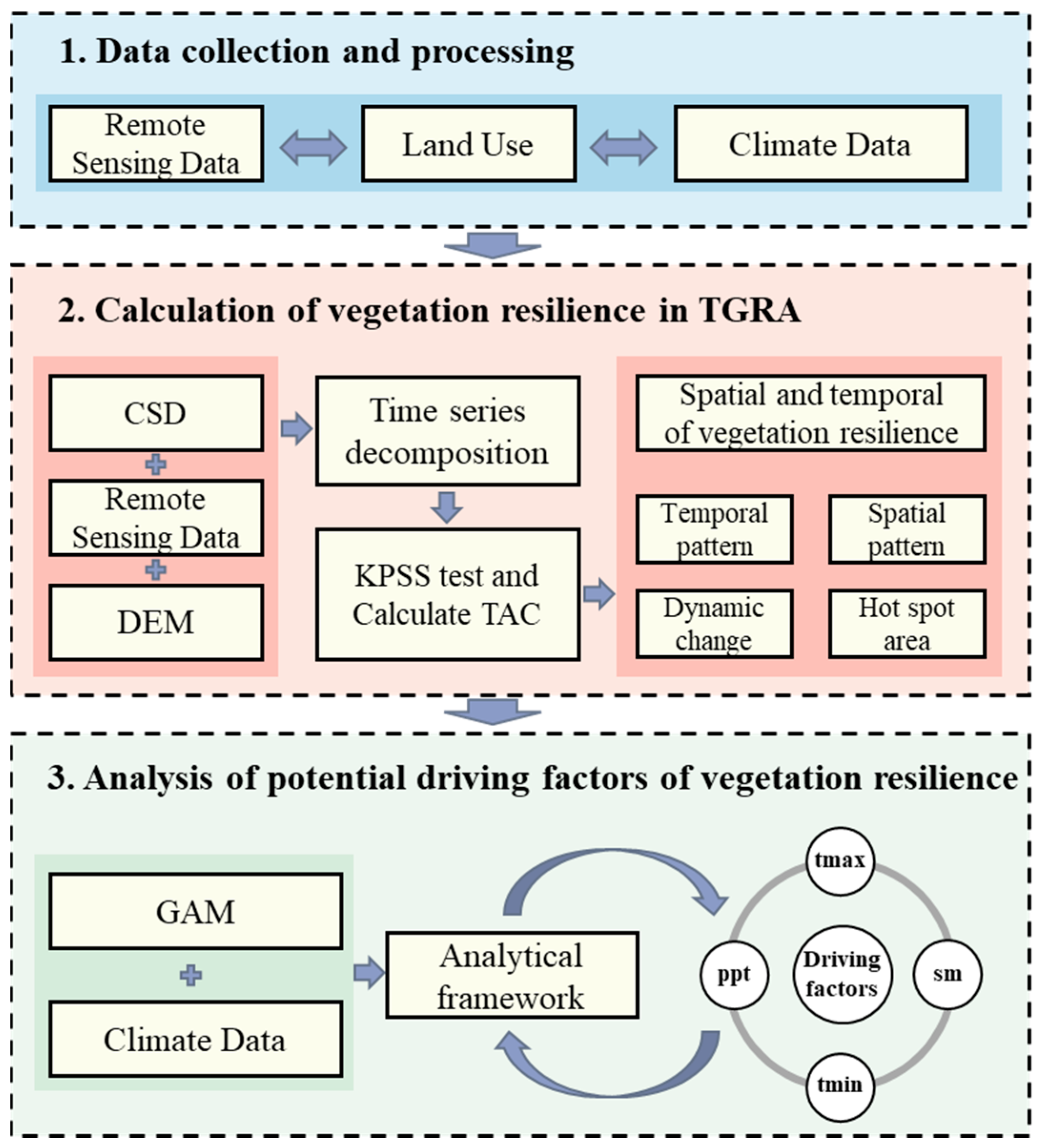
2. Materials and Methods

2.1. Research Area

The Three Gorges Reservoir Area (TGRA) is located at the middle and lower reaches of the Yangtze River [27,29,30,31], involving 30 counties of Chongqing Municipality and Hubei Province, covering 106°16′–111°28′E and 28°56′–31°44′N, with a total area of approximately 58,000 km2 (Figure 1). The TGRA was formed due to the construction of the Three Gorges Dam (TGD), with water impoundment beginning in 2003 and reaching its final level of 175 m in 2010 [29]. Geomorphologically, the TGRA is situated at the intersection of three tectonic units. The topography is high in the east and low in the west. Approximately 74% of the TGRA is mountainous, 22% is hilly, and only 4% is plains or dams [32]. The TGRA is situated in a subtropical humid monsoon climate zone. It experiences humid conditions for most of the year, with an annual mean temperature of 17–19 °C. The temperature generally decreases from northwest to southeast. Annual precipitation ranges from 1000 to 1300 mm, with higher values in the southeast and northwest, and lower values in the northeast and southwest [33].
The main vegetation types are warm evergreen coniferous forests, typical deciduous broad-leaved forests, and shrub forests, which account for 48.8%, 16.6%, and 14.5% of the total area of the TGRA, respectively [34]. Human overexploitation has led to serious destruction and disturbance of the original vegetation, and the area of natural forests in the TGRA is very small. With artificial afforestation, the forest species structure in the TGRA has become relatively single [24].

2.2. Remote Sensing Data

The GLASS LAI was generated by the Center for Global Change Data Processing and Analysis at Beijing Normal University. The time range of the GLASS LAI is from 2000 to 2018, with a spatial resolution of 500 m and a temporal resolution of 8 days [7,35]. This product utilizes MODIS surface reflectance data, CYCLOPES LAI, and a weighted fusion of MODIS LAI products, incorporating real LAI generated by general regression neural networks (GRNNs) [36,37]. Combined with the surface vegetation classification data, the MODIS reflectance for 1 year was input into the GRNN, and the LAI for 1 year was output (Table 1). Compared to other global remote sensing LAI products, the time series of the GLASS LAI is longer and has higher precision, which can reflect the overall characteristics of vegetation and is widely used in ecosystem assessment and global vegetation monitoring. All LAI data were processed and aggregated on a monthly basis, with the maximum value for each pixel extracted to generate the synthesized monthly LAI datasets (see Supplementary Figure S1). By doing so, cloud contamination, shadow effects, and aerosol and water vapor effects can be minimized [38,39].
GlobeLand30 was produced by the National Geomatic Center of China as one of the first global 30 m land cover products produced from freely available Landsat imagery [40]. GlobeLand30 covers three periods—2000, 2010, and 2020—and includes 10 types of land cover. GlobeLand30 increased the resolution to 30 m compared with the original 1000 m and 300 m land-cover products, which better showed most human land-use activities and the resulting landscape patterns. It has a wide range of applications in global weather services, sustainable development, research, and planning [41].

2.3. Climate and Soil Data

TerraClimate is a global monthly climate and hydroclimate product for land surface. It uses climate-assisted interpolation to combine high spatial resolution climatological normals from the WorldClim dataset with coarser spatial resolution and time-varying data from CRU TS 4.0 and the Japanese 55-year Reanalysis (JRA-55). Reanalysis is to generate monthly datasets on primary climate variables (e.g., maximum temperature, precipitation accumulation, etc.) and derived variables (e.g., evapotranspiration, runoff, etc.). TerraClimate produces monthly surface water balance datasets using a water balance model that incorporates reference evapotranspiration, precipitation, temperature, and interpolated plant extractable soil water capacity (Table 1) [11,42]. We selected the precipitation (ppt), maximum temperature (tmax), minimum temperature (tmin), and soil moisture (sm) to analyze the potential drivers of vegetation resilience. TerraClimate dataset spatial resolution can capture major regional gradients and key environmental drivers of vegetation resilience, while avoiding overfitting to fine-scale noise or localized anomalies that may not reflect broader ecological processes, especially when combined with finer resolution datasets such as GLASS LAI (500 m) and GlobeLand30 (30 m).

2.4. Data Pre-Processing

Based on the Critical Slowing Down (CSD) and the Disturbance Event Model (DEM), we constructed a vegetation resilience estimation model to understand the Three Gorges Reservoir Area (TGRA) temporal and spatial distribution characteristics and analyze the influence of climate factors on vegetation resilience (Figure 2).
To match all data, we resampled all datasets to a spatial resolution of 0.5° using bilinear interpolation. For climate data, we used monthly data to ensure that it was spatially and temporally consistent with LAI data.
The study concentrated exclusively on disturbances that did not result in regime shifts within ecosystems. We excluded LAI grids that experienced changes in land cover types from 2000 to 2020. This exclusion was based on the observation that these regions underwent ecosystem transitions due to the combined effects of natural disturbances and human activities. There might exist two or more stable ecosystems in these regions throughout the entire monitoring period. Consequently, the calculated vegetation resilience represents an aggregated value from multiple stable systems, which may not be representative of any single system.

2.5. Time Series Decomposition

The CSD theory shows that the system has lost resilience and may, therefore, be tipped more easily into an alternative state. The effect of this slowing down may be measured in stochastically induced fluctuations in the state of the system as increased variance and “memory”. To obtain an accurate estimate of variance or “memory”, it is essential for time series data to be stationary without long-term trends or seasonal periodic patterns. Therefore, it is necessary to effectively remove seasonal and trend information from the time series data to ensure robust results. In this study, season-trend decomposition by LOESS smoothing (with smooth long-term trend and either stable or smoothly varying seasonal pattern) was utilized for the time series decomposition of GLASS LAI [43]. In each grid cell, the GLASS LAI time series was decomposed into seasonal, trend, and remainder components (Supplementary Figures S3 and S4). Among these, the remainder component, which represents fluctuations after removing both seasonal cycles and long-term trends, was used as the primary metric for assessing vegetation resilience. Time series decomposition is of crucial importance. If the seasonal and trend information is not removed, the changes in TAC may merely reflect the long-term evolution of the system rather than serve as an early warning signal for key transitions [3]. This method is not affected by outliers or vacancy values in time series decomposition and has strong applicability to nonlinear trends [44,45]. In this study, the procedure above was implemented in Python 3.9.

2.6. KPSS Test

We used the KPSS unit root test to examine the stationarity of the remainder series. The KPSS test is a nonparametric test method whose principle is to construct LM statistics from the sequence { e ^ t } that removes the intercept and trend terms from the sequence to be tested and assumes the stability of the estimated residual sequence { e ^ t } by checking whether a unit root exists [46]. Specifically, the KPSS assumes that the original time series is stable, and its four confidence intervals and critical values. If the test statistic is greater than the critical value, the null hypothesis is rejected (i.e., the series is not stationary). If the test statistic is less than the critical value, the null hypothesis (that the series is stable) cannot be rejected. KPSS validation was implemented using Python code in this study.

2.7. Critical Slowing Down

The CSD is based on dynamical systems theory and focuses on detecting early warning signals of regime shifts or tipping points in ecosystems. The CSD does not focus on specific disturbance events but rather on the system’s inherent stability properties and its response to small perturbations over time. The CSD theory shows that when the system reaches a critical state, the attraction basin will become smaller, and small perturbations may cause the system to transform and more easily enter another alternative state [12]. The attraction basin is defined as the set of system states from which the system tends to return after being perturbed. Deeper attraction basins are indicative of higher resilience (rapid recovery), whereas shallower attraction basins suggest lower resilience (slower recovery and a greater likelihood of state transition). The decrease in resilience results in a slower recovery rate after the disturbance and an increase in the similarity between the current and previous time periods. This enhanced “memory” ability can be reflected by an increase in lag-1 autocorrelation (TAC) in random fluctuations of the system (Figure 3) [3,47,48]. Critical slowing down is an indicator of low resilience. When the attraction basin is shallow, the recovery rate of the disturbance is slower than when the basin is deep. Slower intrinsic rates within the system cause it to deviate less from its previous state at any given moment, making its behavior more akin to a random walk. This can be detected through increases in TAC. Higher TAC values correspond to lower system resilience, whereas lower TAC values indicate greater system resilience [49,50].
In this study, CSD serves as the theoretical foundation for measuring ecosystem resilience. One of its key indicators is the temporal autocorrelation at lag-1 autocorrelation (TAC), which captures the increasing “memory” of a system. The tendency for current states is to be more similar to preceding ones under reduced resilience. The autocorrelation function (ACF) is a general statistical tool that measures the correlation of a time series with its past values over different time lags. TAC is a specific case of ACF, representing the autocorrelation at lag 1. It is widely used to quantify early warning signals in time series, with higher TAC values typically indicating lower resilience. When calculating vegetation resilience, the long-term trend and seasonality of each pixel time series were first removed to obtain the remainder information (fluctuation information), and the empirical autocorrelation function at lag-1 (ACF1) of the remainder information was calculated to obtain TAC:
T A C = A C F 1 = t = 1 T 1 x t x ¯ x t + 1 x ¯ t = 1 T x t x ¯ 2
where x t represents the value of time series remainder information on time t, x ¯ represents the mean value of time series remainder information, T represents the total length of time series remainder information, and A C F 1 represents the autocorrelation coefficient of lag-1.

2.8. Disturbance Event Model

The Disturbance Event Model (DEM) assessed the maximum anomaly degree (Ms) and the duration from the maximum anomaly to the return to normal range (Rt) for LAI under recoverable conditions, with resilience being calculated by using their ratio (Figure 4) [17,52]. This study defined a situation where LAI fell below the normal floating range (mean ± one standard deviation) as a vegetation anomaly caused by natural disturbances. The multiyear monthly mean value and monthly standard deviation of LAI were utilized to establish the normal fluctuation range of LAI variations. When LAI dropped below this range, the minimum LAI value was identified as the starting point of vegetation recovery. The difference between this minimum LAI value and the lower limit of the floating range at that specific time represents the maximum anomaly degree (Ms) of LAI under recoverable conditions. Concurrently, the time when LAI returns to the normal range marks the end of disturbance recovery. The duration from the start to the end is defined as the time from maximum abnormality to normalization (Rt). The ratio Ms/Rt was then calculated for each disturbance event, representing the pixel-level resilience during each disturbance episode. Given that multiple disturbance events frequently occurred during the monitoring period from 2000 to 2018, we calculated the vegetation resilience for each disturbance event within each pixel individually. We then took the mean value of the vegetation resilience across all disturbance events as the finally result:
M s i j = M E A N j L A I i j l o w e s t β S T D j
R e s i l i e n c e = M s i j R t
R e s i l i e n c e m e a n = R e s i l i e n c e 1 + R e s i l i e n c e 2 + R e s i l i e n c e 3 + + R e s i l i e n c e n n
where Ms represents the maximum amplitude of LAI when it falls below the normal range, indicating the maximum stress that the ecosystem withstands; LAIij(lowest) denotes the lowest LAI in month j and year i during the anomaly period; MEANj refers to the mean LAI for month j in recent decades (2000–2018 for GLASS LAI); β is the parameter used to adjust the normal range, and β is set to 1 in this study; STDj represents the standard deviation of LAI for month j in recent decades (2000–2018 for GLASS LAI); and Rt is the duration required for the recovery of the LAI value from maximum stress back to its mean. Resilience represents the vegetation resilience at a single disturbance event, the calculation method of Resilience2, Resilience3, …… Resiliencen is the same as that of Resilience. Resiliencemean represents the mean vegetation resilience at multiple disturbance events.
Vegetation resilience based on the CSD method was first calculated annually from monthly LAI data for each year between 2000 and 2018. This produced a yearly resilience value per pixel, which was then averaged across the 19-year period to derive a long-term representative resilience estimate. In contrast, for the DEM approach, resilience was computed by averaging recovery rates from all disturbance events identified within each pixel over the entire study period (2000–2018), resulting in a single value per pixel. To enable consistent spatial comparison between the two models, we aggregated the pixel-level resilience values to the county scale by calculating the mean value of all pixels within each county. It allows for a robust and consistent analysis of long-term spatial patterns in vegetation resilience across the TGRA.

2.9. Regression Analysis

The least-squares method was used to simulate the trend of vegetation resilience pixel by pixel in the TGRA over time:
θ s l o p e = n × i = 1 n i × R e s i i = 1 n i i = 1 n R e s i n × i = 1 n i 2 ( i = 1 n i ) 2
Equation (5) calculates the slope of the vegetation resilience trend over time, denoted as θslope, n represents the number of years of simulation, i represents the ordinal number of years, Resi represents the value of vegetation resilience in year i, and θslope reflects the change trend of vegetation resilience in the TGRA.
The Generalized Additive Regression Model (GAM) is an extension of the generalized linear model [7,53]. Hastie and Tibshirani extended the application scope of additive models by combining the properties of generalized linear models with those of additive models and exploiting generalized additive models. We used the GAM model to evaluate the effects of precipitation (ppt), soil moisture (sm), maximum temperature (tmax) and minimum temperature (tmin) on vegetation resilience, which are mathematically described as follows:
f x = α + f 1   ppt + f 2   sm + f 3   tmin + f 4   tmin + ε i
where α stands for general model intercept, f1 to f4 represents precipitation, soil moisture, maximum temperature, and minimum temperature, respectively, and εi represents the random variable. In this study of the TGRA, f(x) is the resilience of the vegetation ecosystem.

3. Results

3.1. Spatial Consistency and Accuracy Assessment of Resilience Metrics: CSD and DEM

The Critical Slowing Down (CSD) and the Disturbance Event Model (DEM) are both based on the concept of resilience, but they differ in their calculation methods and the range of indicators they use. Given the methodological differences between CSD and DEM, a direct comparison was not feasible; instead, we conducted a spatial consistency and accuracy assessment to evaluate the agreement between the two resilience metrics. The results revealed highly relevant patterns between the CSD and DEM, with an R2 value of 0.80 at the district level. Xingshan, Wuxi, and Yiling exhibited high vegetation resilience, whereas Jiangbei, Dadukou, and Nan’an exhibited low vegetation resilience (Figure 5). Additionally, the CSD and DEM showed consistency among the various vegetation types (Figure 6). Forests and shrublands exhibit high resilience, whereas grasslands and wetlands exhibit low resilience (Figure 7). Although there was an overall consistency, some small differences were found between the results from the two models. The CSD showed that Wulong exhibited the eighth-highest vegetation resilience in the TGRA, whereas the DEM showed that Wulong exhibited the third-highest vegetation resilience. Moreover, the CSD showed that Yuzhong exhibited the fourth-lowest vegetation resilience, whereas the DEM showed that Yuzhong exhibited the lowest vegetation resilience.

3.2. Distribution and Dynamics of Vegetation Resilience

The CSD showed that the eastern part of the TGRA, particularly Xingshan, Wuxi, Yiling, and Badong, exhibited high vegetation resilience with low temporal autocorrelation (TAC) values of 0.36, 0.40, 0.40, and 0.42, respectively (Figure 8 and Figure 9). East Shizhu and southern Jiangjin exhibited relatively high vegetation resilience. Low vegetation resilience was observed in Nanan, parts of Yubei, and Shapingba. In addition, there was minimal difference between different vegetation types. Forests presented the highest vegetation resilience, and wetlands presented the lowest vegetation resilience, with TAC values of 0.43 and 0.55, respectively (Figure 7).
Overall, vegetation resilience in the TGRA showed a decreasing trend. Specifically, the vegetation resilience of Jiulongpo, Jiangjin, Shapingba, Jiangbei, and Dadukou presented a significant decreasing trend, with annual TAC change rates of 0.62%, 0.56%, 0.45%, 0.45%, and 0.40%, respectively, whereas Yubei, Fuling, and Xingshan presented slight increasing trends. The vegetation resilience of Dianjun, Yuzhong, and Wuxi showed an upward trend from 2001 to 2018, with TAC change rates of −0.25%, −0.15%, and −0.02%, respectively. In addition, Central Yiling, East Fuling, West Wulong, and South Dianjun showed significant increasing trends in vegetation resilience (Figure 10).
For the different vegetation types, forest, grassland, shrubland, and wetland showed a decreasing trend in resilience, with annual TAC change rates of 0.11%, 0.18%, 0.10%, and 0.05%, respectively. The change rate of grassland resilience increased nearly twice as fast as that of forest and shrubland resilience and was three times faster than that of wetland resilience. Typically, all vegetation types exhibited significantly higher resilience in 2006.

3.3. Potential Driving Factors in Vegetation Resilience

We incorporated four categories of covariates, namely precipitation (ppt), maximum temperature (tmax), minimum temperature (tmin), and soil moisture (sm) to examine the drivers of spatial disparity in vegetation resilience over the TGRA. Because the TGRA was mainly distributed in forests and grasslands, except for a few shrublands and wetlands, we only analyzed the driving factors of forest vegetation and grassland vegetation.
Statistical analysis revealed that ppt, tmax, tmin, and sm were significantly associated with TAC (Figure 11). Specifically, ppt exhibited a fluctuating effect on TAC in the TGRA and forest from 800 mm/yr to 1800 mm/yr. In the range from 800 mm/yr to 1100 mm/yr, ppt exhibited a positive effect on TAC, and the effect decreased as ppt increased. With increasing ppt, the effect became negative from positive, and the negative effect continued to grow until ppt reached 1600 mm/yr. When ppt exceeded 1600 mm/yr, its impact on TAC shifted from negative to positive as ppt increased. Notably, the effect of ppt on grassland was the exact opposite of its effect on the TGRA and forests. Between 800 mm/yr and 1200 mm/yr, ppt exhibited a negative effect on TAC, and the effect decreased as ppt increased. As ppt continued to rise, the effect transitioned from negative to positive and continued to grow until ppt reached 1800 mm/yr, where the positive effect peaked.
In general, the effect of tmax on TAC is predominantly associated with cooling effects. When tmax falls below 30 °C, it has a negative effect on TAC, and the effect decreases with an increase in tmax. When the tmax exceeds 30 °C, the impact of the tmax on TAC changes from negative to positive with increasing tmax. The effects of tmin on TAC in the TGRA, forest, and grassland were different. The effect of tmin on TAC in the TGRA changed from positive to negative with an increase in tmin. Conversely, the effect of tmin on forests changed from negative to positive as tmin increased. The tmin had little effect on grasslands.
Regarding the impact of sm on TAC, when the sm was below 45, the effect on the TGRA TAC and forest TAC was small; however, the effect on grassland TAC was larger. Sm below 45 had a positive effect on grassland TAC. With an increase in sm, the positive effect weakened, and the effect on grassland TAC was almost 0 when the sm was 45. However, when the sm exceeded 45, it exhibited an inhibitory effect on grassland TAC, which intensified with an increase in sm.

4. Discussion

4.1. Monitoring Model of Vegetation Resilience

Since Holling introduced the concept of resilience to ecology in 1973 [54,55], numerous scholars have conducted studies on the measurement and monitoring of vegetation resilience, and many estimation models have been developed to characterize vegetation resilience [54,56,57]. Since controlled experiments are costly and external disturbances are spatially heterogeneous, it is not feasible to periodically monitor large-area natural disturbances through field surveys. In a word, these are the stumbling blocks in vegetation resilience monitoring using the Disturbance Event Model (DEM) on a large scale.
In this study, we used the Critical Slowing Down (CSD) and remote sensing LAI to estimate the internal fluctuations of the vegetation system for resilience monitoring. The CSD does not focus on specific disturbance events but rather on the system’s inherent stability properties and its response to small perturbations over time. Since CSD calculated vegetation resilience in ecosystems that did not undergo transitions, pixels representing ecosystem transitions between 2000 and 2018 were excluded from this study. The excluded area is relatively small, accounting for only 1.40% of the total study area (Supplementary Figure S2). The CSD shows that when the intrinsic rate of the vegetation system slows down, it is less different from the previous state at any time, and the vegetation system at the current moment is more like the previous moment. The lag-1 autocorrelation is selected as an indicator to represent the similarity between the current moment and the previous moment in this study. The higher the similarity, the greater the autocorrelation and the lower the corresponding vegetation resilience. The lag 2 or lag n contains more complex information, and the current state of the reaction system is not only dependent on the recent past state but is also influenced by multiple past states over a longer period. In practice, whether lag 2 or lag n quantitative calculation of vegetation resilience is reasonable remains to be verified [3,51,58,59,60,61,62,63]. The CSD is used to predict potential regime shifts or tipping points in ecosystems, such as transitions from forest to grassland or coral reef collapse. It is more focused on early warning signals rather than post-disturbance recovery.
We performed a correlation analysis between the resilience estimates derived from the DEM and those obtained from the CSD method to assess their spatial agreement. The DEM focuses on quantifying resilience by analyzing specific disturbance events and the recovery process. DEM is well suited for studying ecosystems with clear disturbance–recovery cycles, such as vegetation responses to droughts, floods, or other discrete events. A low ratio in the DEM indicates a long recovery time under the same intensity, which indicates low resilience. For the selection of the β parameter in the DEM calculation formula, we utilized a landslide case study from Fengjie in 2017 and constructed a DEM schematic diagram based on Leaf Area Index (LAI) data. Our analysis revealed that setting the β parameter to 1 allowed for clear monitoring of the onset and cessation of disturbances (Supplementary Figure S5). The correlation results show that the CSD is negatively correlated with DEM, indicating that the CSD has good applicability in the TGRA.
In addition to models, data are also a grand challenge in monitoring vegetation resilience [64,65]. One of the main difficulties is selecting an appropriate parameter to characterize vegetation variation. Among advanced remote sensing products, LAI can represent the total plant leaf area per unit of land area accurately, thereby avoiding the saturation issue of NDVI in high-value areas and possessing practical physical significance [35,66,67,68]. GPP and biomass are typically derived from LAI, NDVI, or other vegetation indices through statistical modeling [4,57,69], resulting in reduced accuracy. Thus, the LAI was selected to monitor vegetation resilience in this study.

4.2. Dynamics of Vegetation Resilience

The global pattern of vegetation resilience indicates that in Asia the boreal forest belt in northern Asia and the eastern and northeastern regions of China are among the most vulnerable areas [10,14,18,54,70,71,72] facing significant ecological pressures. Recent research also highlights increased vulnerability in southwest China [73], which aligns with our findings. Our study reveals that most of the TGRA regions show high TAC values, reflecting low vegetation resilience.
To further compare the vegetation resilience of different land-cover types in the TGRA with their global counterparts, we examined global patterns of biome sensitivity and resilience. Forests in the TGRA demonstrated the highest resilience, consistent with global observations that tropical and subtropical evergreen broadleaf forests generally possess strong adaptive capacity to climate change due to high biodiversity and productivity [37,74,75,76]. In northeastern TGRA districts (e.g., Xingshan, Wuxi), forest cover exceeds 80%, contributing to higher Leaf Area Index (LAI) and lower TAC values, indicating stronger resilience. This confirmed that high biome diversity and productivity are helpful for ecosystems recovering from external disturbances. Grasslands in the TGRA exhibited lower resilience, especially under high soil moisture conditions. Excessive humidity conditions may lead to hypoxia or reduced physiological activities in the root zone, inhibiting the resilience of the grassland. This aligns with findings that temperate and mountain grasslands are highly sensitive to climatic stress [12,14]. Shrublands in the TGRA showed moderate resilience, consistent with their role as intermediate successional communities, as also observed in Mediterranean and subtropical mountain ecosystems [14,77].
Previous studies have indicated that the dynamics of vegetation resilience are highly heterogeneous on a global scale [14], whereas the current study showed a decreasing trend in vegetation resilience in the TGRA. In recent years, the temperature in the TGRA has continued to rise [78,79], leading to significant changes in land use [65,74,80,81] and an increasingly fragile ecological environment [25,82,83,84]. Our study found similar results, showing that overall vegetation resilience in the TGRA exhibited a decreasing trend. Although Dianjun, Yuzhong, and Wuxi exhibited an upward trend from 2001 to 2018, Dianjun and Yuzhong are in the downtown area, and the ecosystems are highly artificially managed, which is not the focus of this study. In this study, vegetation resilience monitoring was focused on the process of vegetation recovery from natural disturbances.

4.3. The Effects of Potential Drivers

Vegetation resilience may be affected by several factors, such as precipitation, temperature, soil conditions, biodiversity, and fire [79,85,86]. However, due to data limitations, many existing studies have primarily focused on precipitation and temperature as the main influencing factors, with less emphasis on other potential drivers [8,20,66,87]. In this study, we have broadened the scope of analysis to include driving factors such as soil moisture (sm) in addition to precipitation and temperature to analyze their effects on vegetation resilience.
Precipitation (ppt) has been identified as a significant factor influencing vegetation resilience in tropical forests [18,20,74,88,89]. This conclusion was confirmed in the TGRA. Compared with tropical rainforests, the TGRA is located in a temperate zone, where the impact of ppt on vegetation resilience is primarily focused between 800 mm and 1600 mm. Similar to tropical rainforests, an increase in ppt under low-precipitation conditions effectively enhances vegetation resilience [57,90]. However, under high-precipitation conditions, while increased ppt typically inhibits vegetation resilience in tropical regions, the TGRA exhibits a trend of initial inhibition followed by enhancement. Thus, ppt is closely related to vegetation resilience. Extrapolating indirectly from the global probability density of forests, the probability of finding tropical forests decreases sharply when the mean annual precipitation is less than 1500 mm [10,87,91].
Excluding boreal forests and temperate grasslands, temperature exerts a more significant influence on vegetation resilience than precipitation in other biomes [14,92,93]. Our study indicates that the response of vegetation resilience to temperature is approximately linear, contrasting with the nonlinear relationship observed for precipitation. The impact of maximum temperature (tmax) on vegetation resilience primarily relates to its cooling effect [7,94]. Notably, negative repercussions on vegetation resilience become evident when the global mean annual temperature increase surpasses 25 °C [67,81,95,96,97]. We discovered that when tmax exceeds 30 °C, its effect on vegetation resilience begins to diminish in the TGRA. Furthermore, the northern ecosystem exhibits a stronger response to increases in tmax compared to those in minimum temperature (tmin) [73,98]. Consistent with our findings, we noted that the influence of tmin on vegetation resilience within the TGRA is relatively weak.
Soil moisture (sm) have a significant effect on vegetation resilience. As soil moisture increases, water availability also rises, resulting in a nonlinear enhancement of vegetation resilience with greater water availability [4,22,72,97,99]. Our study further confirms that increased sm effectively enhances vegetation resilience.

4.4. Limitation and Future Research

Our study advances the understanding of the spatio-temporal patterns of vegetation resilience in the TGRA. However, certain uncertainties persist. Firstly, the verification of remote sensing data on a large scale remains limited due to the sparse number of field studies and natural perturbations [42,51,70,95,100,101,102]. Secondly, our study considered precipitation, temperature, and soil moisture as drivers of vegetation resilience, overlooking other factors such as terrain changes, and variations in atmospheric carbon dioxide concentration [56,103,104]. Future monitoring of vegetation resilience can be conducted simultaneously at temporal and spatial scales using better models and considering more comprehensive drivers to improve the accuracy of global resilience measurements.

5. Conclusions

Vegetation resilience has become an important research topic because it is a key parameter affecting the quality and stability of ecosystems. Monitoring the growth state of vegetation under disturbance stress and studying its resilience are of great significance for maintaining the stability and sustainable development of entire ecosystems. Taking the Three Gorges Reservoir Area (TGRA) as an example and based on remote sensing, climate, and soil data, this study employed the Critical Slowing Down (CSD) method to calculate vegetation resilience, utilized the Disturbance Event Model (DEM) to verify the accuracy of the CSD, and analyzed the driving factors affecting vegetation resilience. The spatial and temporal distribution characteristics and factors influencing vegetation resilience in the TGRA were analyzed. The results showed that vegetation resilience in the northeast and some parts of the southern TGRA was high, while vegetation resilience in the central and western regions was low. The vegetation resilience of forests, shrubs, and grasslands was high, whereas that of wetlands was low. Precipitation exhibited a fluctuating effect on vegetation resilience in the TGRA from 800 mm/yr to 1800 mm/yr. The sensitivity of vegetation resilience to temperature was not as strong as its sensitivity to precipitation. The CSD has good applicability in the TGRA. The monitoring and analysis of the vegetation resilience in the TGRA has provided a valuable supplement to the study of vegetation resilience in Asia. It has added a typical case and combined the CSD with the less-applied DEM, validating the accuracy of the CSD and enhancing the application of the DEM. With the continuous development of remote sensing products and technologies, more accurate data and better models and methods can be used to dynamically monitor vegetation resilience on a larger spatiotemporal scale.

Supplementary Materials

The following supporting information can be downloaded at https://www.mdpi.com/article/10.3390/rs17132297/s1, Figure S1. Mean LAI values from 2000 to 2018; Figure S2. Percentage chart of exclusion region and study region; Figure S3. Decomposition results of forest single pixel time series; Figure S4. Decomposition results of grassland single pixel time series; Figure S5. DEM monitoring diagram of landslide area in Fengjie in 2017.

Author Contributions

J.W. developed the study design. L.Z., B.Z., and J.W. collected the data and performed the calculations. L.Z., N.Y., J.X., X.S., and J.W. conducted the data analysis. H.S. and S.L. provided supervision throughout the study. L.Z., N.Y., and J.W. contributed to the manuscript writing. All authors have read and agreed to the published version of the manuscript.

Funding

This work was partially supported by the National Key R&D Program of China (2023YFC3007204-4) and the Natural National Science Foundation of China (42101407).

Data Availability Statement

The authors declare that the data supporting the findings of this study are available in Supplementary Materials.

Conflicts of Interest

The authors declare no conflicts of interest.

References

  1. van Nes, E.H.; Scheffer, M. Slow recovery from perturbations as a generic indicator of a nearby catastrophic shift. Am. Nat. 2007, 169, 738–747. [Google Scholar] [CrossRef]
  2. Carpenter, S.R.; Brock, W.A.; Cole, J.J.; Kitchell, J.F.; Pace, M.L. Leading indicators of trophic cascades. Ecol. Lett. 2008, 11, 128–138. [Google Scholar] [CrossRef]
  3. Scheffer, M.; Bascompte, J.; Brock, W.A.; Brovkin, V.; Carpenter, S.R.; Dakos, V.; Held, H.; van Nes, E.H.; Rietkerk, M.; Sugihara, G. Early-warning signals for critical transitions. Nature 2009, 461, 53–59. [Google Scholar] [CrossRef]
  4. Ponce Campos, G.E.; Moran, M.S.; Huete, A.; Zhang, Y.; Bresloff, C.; Huxman, T.E.; Eamus, D.; Bosch, D.D.; Buda, A.R.; Gunter, S.A.; et al. Ecosystem resilience despite large-scale altered hydroclimatic conditions. Nature 2013, 494, 349–352. [Google Scholar] [CrossRef]
  5. Allen, C.D.; Macalady, A.K.; Chenchouni, H.; Bachelet, D.; McDowell, N.; Vennetier, M.; Kitzberger, T.; Rigling, A.; Breshears, D.D.; Hogg, E.H.; et al. A global overview of drought and heat-induced tree mortality reveals emerging climate change risks for forests. For. Ecol. Manag. 2010, 259, 660–684. [Google Scholar] [CrossRef]
  6. Li, X.; Piao, S.; Wang, K.; Wang, X.; Wang, T.; Ciais, P.; Chen, A.; Lian, X.; Peng, S.; Peñuelas, J. Temporal trade-off between gymnosperm resistance and resilience increases forest sensitivity to extreme drought. Nat. Ecol. Evol. 2020, 4, 1075–1083. [Google Scholar] [CrossRef]
  7. Chen, B.; Wu, S.; Song, Y.; Webster, C.; Xu, B.; Gong, P. Contrasting inequality in human exposure to greenspace between cities of Global North and Global South. Nat. Commun. 2022, 13, 4636. [Google Scholar] [CrossRef]
  8. Veryard, R.; Wu, J.; O’Brien, M.J.; Anthony, R.; Both, S.; Burslem, D.; Chen, B.; Fernandez-Miranda Cagigal, E.; Godfray, H.C.J.; Godoong, E.; et al. Positive effects of tree diversity on tropical forest restoration in a field-scale experiment. Sci. Adv. 2023, 9, eadf0938. [Google Scholar] [CrossRef]
  9. Boulton, C.A.; Good, P.; Lenton, T.M. Early warning signals of simulated Amazon rainforest dieback. Theor. Ecol. 2013, 6, 373–384. [Google Scholar] [CrossRef]
  10. Seddon, A.W.; Macias-Fauria, M.; Long, P.R.; Benz, D.; Willis, K.J. Sensitivity of global terrestrial ecosystems to climate variability. Nature 2016, 531, 229–232. [Google Scholar] [CrossRef]
  11. Abatzoglou, J.T.; Dobrowski, S.Z.; Parks, S.A.; Hegewisch, K.C. TerraClimate, a high-resolution global dataset of monthly climate and climatic water balance from 1958–2015. Sci. Data 2018, 5, 170191. [Google Scholar] [CrossRef]
  12. Gonzalez, P.; Neilson, R.P.; Lenihan, J.M.; Drapek, R.J. Global patterns in the vulnerability of ecosystems to vegetation shifts due to climate change. Glob. Ecol. Biogeogr. 2010, 19, 755–768. [Google Scholar] [CrossRef]
  13. Harris, A.; Carr, A.S.; Dash, J. Remote sensing of vegetation cover dynamics and resilience across southern Africa. Int. J. Appl. Earth Obs. Geoinf. 2014, 28, 131–139. [Google Scholar] [CrossRef]
  14. Feng, Y.; Su, H.; Tang, Z.; Wang, S.; Zhao, X.; Zhang, H.; Ji, C.; Zhu, J.; Xie, P.; Fang, J. Reduced resilience of terrestrial ecosystems locally is not reflected on a global scale. Commun. Earth Environ. 2021, 2, 88. [Google Scholar] [CrossRef]
  15. Davidson, E.A.; de Araújo, A.C.; Artaxo, P.; Balch, J.K.; Brown, I.F.; Bustamante, M.M.C.; Coe, M.T.; DeFries, R.S.; Keller, M.; Longo, M.; et al. The Amazon basin in transition. Nature 2012, 481, 321–328. [Google Scholar] [CrossRef]
  16. Zhu, Q.; Chen, H.; Peng, C.; Liu, J.; Piao, S.; He, J.-S.; Wang, S.; Zhao, X.; Zhang, J.; Fang, X.; et al. An early warning signal for grassland degradation on the Qinghai-Tibetan Plateau. Nat. Commun. 2023, 14, 6406. [Google Scholar] [CrossRef]
  17. Díaz-Delgado, R.; Lloret, F.; Pons, X.; Terradas, J. Satellite evidence of decreasing resilience in Mediterranean plant communities after recurrent wildfires. Ecology 2002, 83, 2293–2303. [Google Scholar] [CrossRef]
  18. Zscheischler, J.; Mahecha, M.; von Buttlar, J. A few extreme events dominate global interannual variability in gross primary production. Environ. Res. Lett. 2014, 9, 035001. [Google Scholar] [CrossRef]
  19. Gunderson, L.H. Ecological Resilience—In Theory and Application. Annu. Rev. Ecol. Syst. 2000, 31, 425–439. [Google Scholar] [CrossRef]
  20. Verbesselt, J.; Umlauf, N.; Hirota, M.; Holmgren, M.; Van Nes, E.H.; Herold, M.; Zeileis, A.; Scheffer, M. Remotely sensed resilience of tropical forests. Nat. Clim. Change 2016, 6, 1028–1031. [Google Scholar] [CrossRef]
  21. Huntingford, C.; Zelazowski, P.; Galbraith, D.; Mercado, L.M.; Sitch, S.; Fisher, R.; Lomas, M.; Walker, A.P.; Jones, C.D.; Booth, B.B.B.; et al. Simulated resilience of tropical rainforests to CO2-induced climate change. Nat. Geosci. 2013, 6, 268–273. [Google Scholar] [CrossRef]
  22. Smith, T.; Traxl, D.; Boers, N. Empirical evidence for recent global shifts in vegetation resilience. Nat. Clim. Change 2022, 12, 477–484. [Google Scholar] [CrossRef]
  23. Wu, J.; Huang, J.; Han, X.; Gao, X.; He, F.; Jiang, M.; Jiang, Z.; Primack, R.B.; Shen, Z. The Three Gorges Dam: An ecological perspective. Front. Ecol. Environ. 2004, 2, 241–248. [Google Scholar] [CrossRef]
  24. Wen, Z.; Yang, H.; Zhang, C.; Shao, G.; Wu, S. Remotely Sensed Mid-Channel Bar Dynamics in Downstream of the Three Gorges Dam, China. Remote Sens. 2020, 12, 409. [Google Scholar] [CrossRef]
  25. Lai, Z.; Li, L.; Tao, Z.; Li, T.; Shi, X.; Li, J.; Li, X. Spatio-Temporal Evolution and Influencing Factors of Ecological Well-Being Performance from the Perspective of Strong Sustainability: A Case Study of the Three Gorges Reservoir Area, China. Int. J. Environ. Res. Public Health 2023, 20, 1810. [Google Scholar] [CrossRef]
  26. Zhang, J.; Xu, Q. The Changing Trend of Biodiversity in the Three Gorges Reservoir Area and Its Protection Countermeasures. The situation of biodiversity changes in the Three Gorges Reservoir area and its conservation countermeasures. Trop. Geogr. 1997, 17, 412–418. [Google Scholar]
  27. Huang, C.; Huang, X.; Peng, C.; Zhou, Z.; Teng, M.; Wang, P. Land use/cover change in the Three Gorges Reservoir area, China: Reconciling the land use conflicts between development and protection. Catena 2019, 175, 388–399. [Google Scholar] [CrossRef]
  28. Liu, S.; Liao, Q.; Xiao, M.; Zhao, D.; Huang, C. Spatial and Temporal Variations of Habitat Quality and Its Response of Landscape Dynamic in the Three Gorges Reservoir Area, China. Int. J. Environ. Res. Public Health 2022, 19, 3594. [Google Scholar] [CrossRef]
  29. Shen, G.; Xie, Z. Three Gorges Project: Chance and challenge. Science 2004, 304, 681. [Google Scholar] [CrossRef]
  30. Xiao, Y.; Xiao, Q.; Xiong, Q.; Yang, Z. Effects of Ecological Restoration Measures on Soil Erosion Risk in the Three Gorges Reservoir Area Since the 1980s. GeoHealth 2020, 4, e2020GH000274. [Google Scholar] [CrossRef]
  31. Song, Z.; Liang, S.; Feng, L.; He, T.; Song, X.-P.; Zhang, L. Temperature changes in Three Gorges Reservoir Area and linkage with Three Gorges Project. J. Geophys. Res. Atmos. 2017, 122, 4866–4879. [Google Scholar] [CrossRef]
  32. Bao, Y.; Gao, P.; He, X. The water-level fluctuation zone of Three Gorges Reservoir—A unique geomorphological unit. Earth-Sci. Rev. 2015, 150, 14–24. [Google Scholar] [CrossRef]
  33. Miller, N.L.; Jin, J.; Tsang, C.F. Local climate sensitivity of the Three Gorges Dam. Geophys. Res. Lett. 2005, 32. [Google Scholar] [CrossRef]
  34. Zhu, Z.; Chen, Z.; Li, L.; Shao, Y. Response of dominant plant species to periodic flooding in the riparian zone of the Three Gorges Reservoir (TGR), China. Sci. Total Environ. 2020, 747, 141101. [Google Scholar] [CrossRef]
  35. Liang, S.; Cheng, J.; Jia, K.; Jiang, B.; Liu, Q.; Xiao, Z.; Yao, Y.; Yuan, W.; Zhang, X.; Zhao, X.; et al. The Global Land Surface Satellite (GLASS) Product Suite. Bull. Am. Meteorol. Soc. 2021, 102, E323–E337. [Google Scholar] [CrossRef]
  36. Ives, A.R. Measuring Resilience in Stochastic Systems. Ecol. Monogr. 1995, 65, 217–233. [Google Scholar] [CrossRef]
  37. Hirota, M.; Holmgren, M.; Van Nes, E.H.; Scheffer, M. Global resilience of tropical forest and savanna to critical transitions. Science 2011, 334, 232–235. [Google Scholar] [CrossRef]
  38. Bacour, C.; Baret, F.; Béal, D.; Weiss, M.; Pavageau, K. Neural network estimation of LAI, fAPAR, fCover and LAI × C ab, from top of canopy MERIS reflectance data: Principles and validation. Remote Sens. Environ. 2006, 105, 313–325. [Google Scholar] [CrossRef]
  39. Qin, J.; Liang, S.; Li, X.; Wang, J. Development of the Adjoint Model of a Canopy Radiative Transfer Model for Sensitivity Study and Inversion of Leaf Area Index. IEEE Trans. Geosci. Remote Sens. 2008, 46, 2028–2037. [Google Scholar] [CrossRef]
  40. Fonte, C.; Minghini, M.; Patriarca, J.; Antoniou, V.; See, L.; Skopeliti, A. Generating Up-to-Date and Detailed Land Use and Land Cover Maps Using OpenStreetMap and GlobeLand30. ISPRS Int. J. Geo-Inf. 2017, 6, 125. [Google Scholar] [CrossRef]
  41. Xie, H.; Tong, X.; Meng, W.; Liang, D.; Wang, Z.; Shi, W. A Multilevel Stratified Spatial Sampling Approach for the Quality Assessment of Remote-Sensing-Derived Products. IEEE J. Sel. Top. Appl. Earth Obs. Remote Sens. 2015, 8, 4699–4713. [Google Scholar] [CrossRef]
  42. Brando, P.M.; Balch, J.K.; Nepstad, D.C.; Morton, D.C.; Putz, F.E.; Coe, M.T.; Silverio, D.; Macedo, M.N.; Davidson, E.A.; Nobrega, C.C.; et al. Abrupt increases in Amazonian tree mortality due to drought-fire interactions. Proc. Natl. Acad. Sci. USA 2014, 111, 6347–6352. [Google Scholar] [CrossRef]
  43. Jiang, B.; Liang, S.; Wang, J.; Xiao, Z. Modeling MODIS LAI time series using three statistical methods. Remote Sens. Environ. 2010, 114, 1432–1444. [Google Scholar] [CrossRef]
  44. Jesús, R.; Rosario, R.; Jorge, R.-M.; Federico, F.-G.; Rosa, P.-B. Modeling pollen time series using seasonal-trend decomposition procedure based on LOESS smoothing. Int. J. Biometeorol. 2017, 61, 335–348. [Google Scholar]
  45. Ben Abbes, A.; Bounouh, O.; Farah, I.R.; de Jong, R.; Martínez, B. Comparative study of three satellite image time-series decomposition methods for vegetation change detection. Eur. J. Remote Sens. 2018, 51, 607–615. [Google Scholar] [CrossRef]
  46. Kwiatkowski, D.; Phillips, P.C.; Schmidt, P.; Shin, Y. Testing the null hypothesis of stationarity against the alternative of a unit root: How sure are we that economic time series have a unit root? J. Econom. 1992, 54, 159–178. [Google Scholar] [CrossRef]
  47. Brock, W.A.; Carpenter, S.R. Early warnings of regime shift when the ecosystem structure is unknown. PLoS ONE 2012, 7, e45586. [Google Scholar] [CrossRef]
  48. Carpenter, S.R.; Brock, W.A. Early warnings of regime shifts in spatial dynamics using the discrete Fourier transform. Ecosphere 2010, 1, 1–15. [Google Scholar] [CrossRef]
  49. Held, H.; Kleinen, T. Detection of climate system bifurcations by degenerate fingerprinting. Geophys. Res. Lett. 2004, 31. [Google Scholar] [CrossRef]
  50. Hu, Z.M.; Guo, Q.; Li, S.G.; Piao, S.L.; Knapp, P.; Ciais, P.; Li, X.R.; Yu, G.R. Shifts in the dynamics of productivity signal ecosystem state transitions at the biome-scale. Ecol. Lett. 2018, 21, 1457–1466. [Google Scholar] [CrossRef]
  51. Scheffer, M.; Carpenter, S.R.; Lenton, T.M.; Bascompte, J.; Brock, W.; Dakos, V.; van de Koppel, J.; van de Leemput, I.A.; Levin, S.A.; van Nes, E.H.; et al. Anticipating critical transitions. Science 2012, 338, 344–348. [Google Scholar] [CrossRef]
  52. Jones, M.O.; Jones, L.A.; Kimball, J.S.; McDonald, K.C. Satellite passive microwave remote sensing for monitoring global land surface phenology. Remote Sens. Environ. 2011, 115, 1102–1114. [Google Scholar] [CrossRef]
  53. Carpenter, S.R.; Lathrop, R.C. Probabilistic Estimate of a Threshold for Eutrophication. Ecosystems 2008, 11, 601–613. [Google Scholar] [CrossRef]
  54. Folke, C.; Carpenter, S. Resilience Thinking: Integrating Resilience, Adaptability and Transformability. Ecol. Soc. 2010, 15, 20. [Google Scholar] [CrossRef]
  55. Holling, C.S. Resilience and Stability of Ecological Systems. Annu. Rev. Ecol. Syst. 1973, 4. [Google Scholar] [CrossRef]
  56. Folke, C. Resilience: The emergence of a perspective for social-ecological systems analyses. Glob. Environ. Change 2006, 16, 253–267. [Google Scholar] [CrossRef]
  57. Yan, H.; Zhan, J.; Zhang, T. Resilience of Forest Ecosystems and Its Influencing Factors. Procedia Environ. Sci. 2011, 10, 2201–2206. [Google Scholar] [CrossRef]
  58. Dakos, V.; van Nes, E.H.; Scheffer, M. Flickering as an early warning signal. Theor. Ecol. 2013, 6, 309–317. [Google Scholar] [CrossRef]
  59. Dakos, V.; Carpenter, S.R.; Brock, W.A.; Ellison, A.M.; Guttal, V.; Ives, A.R.; Kefi, S.; Livina, V.; Seekell, D.A.; van Nes, E.H.; et al. Methods for detecting early warnings of critical transitions in time series illustrated using simulated ecological data. PLoS ONE 2012, 7, e41010. [Google Scholar] [CrossRef]
  60. Dakos, V.; Scheffer, M.; van Nes, E. Slowing down as an early warning signal for abrupt climate change. Proc. Natl. Acad. Sci. USA 2008, 105, 14308–14312. [Google Scholar] [CrossRef]
  61. Dakos, V.; Kefi, S.; Rietkerk, M.; van Nes, E.H.; Scheffer, M. Slowing down in spatially patterned ecosystems at the brink of collapse. Am. Nat. 2011, 177, E153–E166. [Google Scholar] [CrossRef]
  62. Dakos, V.; van Nes, E.H.; Donangelo, R.; Fort, H.; Scheffer, M. Spatial correlation as leading indicator of catastrophic shifts. Theor. Ecol. 2009, 3, 163–174. [Google Scholar] [CrossRef]
  63. Scheffer, M.; Hirota, M.; Holmgren, M.; Van Nes, E.H.; Chapin, F.S., 3rd. Thresholds for boreal biome transitions. Proc. Natl. Acad. Sci. USA 2012, 109, 21384–21389. [Google Scholar] [CrossRef]
  64. Wilson, R. Advanced remote sensing: Terrestrial information extraction and applications, by Shunlin Liang, Xiaowen Li and Jindi Wang. Int. J. Remote Sens. 2013, 34, 5262–5263. [Google Scholar] [CrossRef]
  65. Cantarello, E.; Newton, A.C.; Martin, P.A.; Evans, P.M.; Gosal, A.; Lucash, M.S. Quantifying resilience of multiple ecosystem services and biodiversity in a temperate forest landscape. Ecol. Evol. 2017, 7, 9661–9675. [Google Scholar] [CrossRef]
  66. Wu, J.; Liang, S. Assessing Terrestrial Ecosystem Resilience Using Satellite Leaf Area Index. Remote Sens. 2020, 12, 595. [Google Scholar] [CrossRef]
  67. Bai, Y.; Han, X.; Wu, J.; Chen, Z.; Li, L. Ecosystem stability and compensatory effects in the Inner Mongolia grassland. Nature 2004, 431, 181–184. [Google Scholar] [CrossRef]
  68. Li, W.F.; Cao, Q.W.; Lang, K.; Wu, J.S. Linking potential heat source and sink to urban heat island: Heterogeneous effects of landscape pattern on land surface temperature. Sci. Total Environ. 2017, 586, 457–465. [Google Scholar] [CrossRef]
  69. Zhao, X.; Yi, P.; Xia, J.; He, W.; Gao, X. Temporal and spatial analysis of the ecosystem service values in the Three Gorges Reservoir area of China based on land use change. Environ. Sci. Pollut. Res. 2022, 29, 26549–26563. [Google Scholar] [CrossRef]
  70. Fleischer, K.; Rebel, K.T.; van der Molen, M.K.; Erisman, J.W.; Wassen, M.J.; van Loon, E.E.; Montagnani, L.; Gough, C.M.; Herbst, M.; Janssens, I.A.; et al. The contribution of nitrogen deposition to the photosynthetic capacity of forests. Glob. Biogeochem. Cycles 2013, 27, 187–199. [Google Scholar] [CrossRef]
  71. Flores, B.M.; Holmgren, M.; Xu, C.; van Nes, E.H.; Jakovac, C.C.; Mesquita, R.C.G.; Scheffer, M. Floodplains as an Achilles’ heel of Amazonian forest resilience. Proc. Natl. Acad. Sci. USA 2017, 114, 4442–4446. [Google Scholar] [CrossRef]
  72. Forzieri, G.; Dakos, V.; McDowell, N.G.; Ramdane, A.; Cescatti, A. Emerging signals of declining forest resilience under climate change. Nature 2022, 608, 534–539. [Google Scholar] [CrossRef]
  73. Anderegg, W.R.; Anderegg, L.D.; Berry, J.A.; Field, C.B. Loss of whole-tree hydraulic conductance during severe drought and multi-year forest die-off. Oecologia 2014, 175, 11–23. [Google Scholar] [CrossRef]
  74. Barati, A.A.; Zhoolideh, M.; Azadi, H.; Lee, J.-H.; Scheffran, J. Interactions of land-use cover and climate change at global level: How to mitigate the environmental risks and warming effects. Ecol. Indic. 2023, 146, 109829. [Google Scholar] [CrossRef]
  75. Barnosky, A.D.; Hadly, E.A.; Bascompte, J.; Berlow, E.L.; Brown, J.H.; Fortelius, M.; Getz, W.M.; Harte, J.; Hastings, A.; Marquet, P.A.; et al. Approaching a state shift in Earth’s biosphere. Nature 2012, 486, 52–58. [Google Scholar] [CrossRef]
  76. Burgan, H.I.; Icaga, Y.; Bostanoglu, Y.; Kilit, M. Water Quality Tendency of Akarçay River Between 2006–2011. Pamukkale Univ. J. Eng. Sci. 2013, 19, 127–132. [Google Scholar] [CrossRef]
  77. Li, D.; Wu, S.; Liu, L.; Zhang, Y.; Li, S. Vulnerability of the global terrestrial ecosystems to climate change. Glob. Change Biol. 2018, 24, 4095–4106. [Google Scholar] [CrossRef]
  78. Cote, I.M.; Darling, E.S. Rethinking ecosystem resilience in the face of climate change. PLoS Biol. 2010, 8, e1000438. [Google Scholar] [CrossRef]
  79. Donangelo, R.; Fort, H.; Dakos, V.; Scheffer, M.; Van Nes, E.H. Early Warnings for Catastrophic Shifts in Ecosystems: Comparison Between Spatial and Temporal Indicators. Int. J. Bifurc. Chaos 2012, 20, 315–321. [Google Scholar] [CrossRef]
  80. Holm, A. The use of time-integrated NOAA NDVI data and rainfall to assess landscape degradation in the arid shrubland of Western Australia. Remote Sens. Environ. 2003, 85, 145–158. [Google Scholar] [CrossRef]
  81. MacDougall, A.S.; Esch, E.; Chen, Q.; Carroll, O.; Bonner, C.; Ohlert, T.; Siewert, M.; Sulik, J.; Schweiger, A.K.; Borer, E.T.; et al. Widening global variability in grassland biomass since the 1980s. Nat. Ecol. Evol. 2024, 8, 1877–1888. [Google Scholar] [CrossRef]
  82. Carpenter, S.R.; Brock, W.A. Rising variance: A leading indicator of ecological transition. Ecol. Lett. 2006, 9, 311–318. [Google Scholar] [CrossRef]
  83. Scheffer, M.; Carpenter, S.R.; Dakos, V.; van Nes, E.H. Generic Indicators of Ecological Resilience: Inferring the Chance of a Critical Transition. Annu. Rev. Ecol. Evol. Syst. 2015, 46, 145–167. [Google Scholar] [CrossRef]
  84. Seekell, D.A.; Carpenter, S.R.; Pace, M.L. Conditional Heteroscedasticity as a Leading Indicator of Ecological Regime Shifts. Am. Nat. 2011, 178, 442–451. [Google Scholar] [CrossRef]
  85. Staal, A.; Tuinenburg, O.A.; Bosmans, J.H.C.; Holmgren, M.; van Nes, E.H.; Scheffer, M.; Zemp, D.C.; Dekker, S.C. Forest-rainfall cascades buffer against drought across the Amazon. Nat. Clim. Change 2018, 8, 539–543. [Google Scholar] [CrossRef]
  86. Woodward, C.L. Soil compaction and topsoil removal effects on soil properties and seedling growth in Amazonian Ecuador. For. Ecol. Manag. 1996, 82, 197–209. [Google Scholar] [CrossRef]
  87. Seidl, R.; Thom, D.; Kautz, M.; Martin-Benito, D.; Peltoniemi, M.; Vacchiano, G.; Wild, J.; Ascoli, D.; Petr, M.; Honkaniemi, J.; et al. Forest disturbances under climate change. Nat. Clim. Change 2017, 7, 395–402. [Google Scholar] [CrossRef]
  88. Boers, N. Observation-based early-warning signals for a collapse of the Atlantic Meridional Overturning Circulation. Nat. Clim. Change 2021, 11, 680–688. [Google Scholar] [CrossRef]
  89. Zhou, L.; Tian, Y.; Myneni, R.B.; Ciais, P.; Saatchi, S.; Liu, Y.Y.; Piao, S.; Chen, H.; Vermote, E.F.; Song, C.; et al. Widespread decline of Congo rainforest greenness in the past decade. Nature 2014, 509, 86–90. [Google Scholar] [CrossRef]
  90. Zemp, D.C.; Schleussner, C.F.; Barbosa, H.M.; Hirota, M.; Montade, V.; Sampaio, G.; Staal, A.; Wang-Erlandsson, L.; Rammig, A. Self-amplified Amazon forest loss due to vegetation-atmosphere feedbacks. Nat. Commun. 2017, 8, 14681. [Google Scholar] [CrossRef]
  91. Xu, C.; Wang, H.; Liu, Q.; Wang, B. Alternative stable states and tipping points of ecosystems. Biodivers. Sci. 2020, 28, 1417–1430. [Google Scholar] [CrossRef]
  92. Feng, H.; Liu, K.; Wang, S.; Wang, Z. A Combination of Ecology Environment and View: The Ideal Green Highway Construction-Highway Eco-Landscape Planning and Constructing in Qinling Region. In Proceedings of the 2016 5th International Conference on Education and Education Management (Eem 2016), Nadi, Fiji, 20–21 December 2016; Volume 92, pp. 408–412. [Google Scholar]
  93. Feng, L.; Zhang, Z.; Ma, Y.; Sun, Y.; Du, Q.; Williams, P.; Drewry, J.; Luck, B. Multitask Learning of Alfalfa Nutritive Value from UAV-Based Hyperspectral Images. IEEE Geosci. Remote Sens. Lett. 2022, 19, 1–5. [Google Scholar] [CrossRef]
  94. Chen, Y.; Zhang, T.B.; Zhou, X.B.; Li, J.J.; Yi, G.H.; Bie, X.J.; Hu, J.; Wen, B. Ecological sensitivity and its driving factors in the area along the Sichuan-Tibet Railway. Environ. Dev. Sustain. 2024, 26, 20189–20208. [Google Scholar] [CrossRef]
  95. Poorter, L.; Bongers, F.; Aide, T.M.; Almeyda Zambrano, A.M.; Balvanera, P.; Becknell, J.M.; Boukili, V.; Brancalion, P.H.; Broadbent, E.N.; Chazdon, R.L.; et al. Biomass resilience of Neotropical secondary forests. Nature 2016, 530, 211–214. [Google Scholar] [CrossRef]
  96. de Vries, F.T.; Liiri, M.E.; Bjørnlund, L.; Bowker, M.A.; Christensen, S.; Setälä, H.M.; Bardgett, R.D. Land use alters the resistance and resilience of soil food webs to drought. Nat. Clim. Change 2012, 2, 276–280. [Google Scholar] [CrossRef]
  97. Smith, T.; Boers, N. Global vegetation resilience linked to water availability and variability. Nat. Commun. 2023, 14, 498. [Google Scholar] [CrossRef]
  98. Lamothe, K.A.; Somers, K.M.; Jackson, D.A. Linking the ball-and-cup analogy and ordination trajectories to describe ecosystem stability, resistance, and resilience. Ecosphere 2019, 10, e02629. [Google Scholar] [CrossRef]
  99. Wang, Y.; Peng, L.; Yue, Y.; Chen, T. Global Vegetation-Temperature Sensitivity and Its Driving Forces in the 21st Century. Earth’s Future 2024, 12, e2022EF003395. [Google Scholar] [CrossRef]
  100. Walker, T.W.N.; Janssens, I.A.; Weedon, J.T.; Sigurdsson, B.D.; Richter, A.; Peñuelas, J.; Leblans, N.I.W.; Bahn, M.; Bartrons, M.; De Jonge, C.; et al. A systemic overreaction to years versus decades of warming in a subarctic grassland ecosystem. Nat. Ecol. Evol. 2019, 4, 101–108. [Google Scholar] [CrossRef]
  101. Ma, X.; Huete, A.; Moran, S.; Ponce-Campos, G.; Eamus, D. Abrupt shifts in phenology and vegetation productivity under climate extremes. J. Geophys. Res. Biogeosci. 2015, 120, 2036–2052. [Google Scholar] [CrossRef]
  102. Peng, J.; Zong, M.L.; Hu, Y.N.; Liu, Y.X.; Wu, J.S. Assessing Landscape Ecological Risk in a Mining City: A Case Study in Liaoyuan City, China. Sustainability 2015, 7, 8312–8334. [Google Scholar] [CrossRef]
  103. Huang, R.Y.; Yeh, C.H. Development of an assessment framework for green highway construction. J. Chin. Inst. Eng. 2008, 31, 573–585. [Google Scholar] [CrossRef]
  104. Keller, I.; Largiadér, C.R. Recent habitat fragmentation caused by major roads leads to reduction of gene flow and loss of genetic variability in ground beetles. Proc. R. Soc. B Biol. Sci. 2003, 270, 417–423. [Google Scholar] [CrossRef]
Figure 1. The location of the TGRA.
Remotesensing 17 02297 g001
Figure 2. The flow chart of this study.
Remotesensing 17 02297 g002
Figure 3. The schematic of the Critical Slowing Down (CSD) (a,b): Two hypothetical system states showing different attraction basin depths; a deep basin reflects high resilience, while a shallow basin indicates low resilience; (c,d): system responses to perturbations; systems with high resilience return quickly to equilibrium, while systems near tipping points recover slowly; (e,f): lag-1 autocorrelation: increasing lag-1 autocorrelation (TAC) as a system nears critical transition, illustrating slower recovery and enhanced memory [51].
Remotesensing 17 02297 g003
Figure 4. The schematic of the Disturbance Event Model (DEM).
Remotesensing 17 02297 g004
Figure 5. The disturbance event model vegetation resilience of the TGRA from 2000 to 2018.
Remotesensing 17 02297 g005
Figure 6. Correlation between the CSD and the DEM in the TGRA.
Remotesensing 17 02297 g006
Figure 7. Resilience of different land types in the TGRA.
Remotesensing 17 02297 g007
Figure 8. The critical slowing down resilience in the TGRA from 2000 to 2018.
Remotesensing 17 02297 g008
Figure 9. Resilience of the TGRA from 2000 to 2018.
Remotesensing 17 02297 g009
Figure 10. The critical slowing down resilience change rate of TGRA from 2000 to 2018.
Remotesensing 17 02297 g010
Figure 11. Relationship between TAC of forest and grassland and ppt, sm, tmax, and tmin.
Remotesensing 17 02297 g011
Table 1. Overview of data properties.
DataPeriodSpatial
Resolution
Temporal
Resolution
GLASS LAI2000–2018500 m8 days
GlobeLand302000, 2010, 202030 m
TerraClimate1958–20220.5°1 month
Disclaimer/Publisher’s Note: The statements, opinions and data contained in all publications are solely those of the individual author(s) and contributor(s) and not of MDPI and/or the editor(s). MDPI and/or the editor(s) disclaim responsibility for any injury to people or property resulting from any ideas, methods, instructions or products referred to in the content.

