Multi-Neighborhood Sparse Feature Selection for Semantic Segmentation of LiDAR Point Clouds

Abstract

LiDAR point clouds, as direct carriers of 3D spatial information, comprehensively record the geometric features and spatial topological relationships of object surfaces, providing intelligent systems with rich 3D scene representation capability. However, current point cloud semantic segmentation methods primarily extract features through operations such as convolution and pooling, yet fail to adequately consider sparse features that significantly influence the final results of point cloud-based scene perception, resulting in insufficient feature representation capability. To address these problems, a sparse feature dynamic graph convolutional neural network, abbreviated as SFDGNet, is constructed in this paper for LiDAR point clouds of complex scenes. In the context of this paper, sparse features refer to feature representations in which only a small number of activation units or channels exhibit significant responses during the forward pass of the model. First, a sparse feature regularization method was used to motivate the network model to learn the sparsified feature weight matrix. Next, a split edge convolution module, abbreviated as SEConv, was designed to extract the local features of the point cloud from multiple neighborhoods by dividing the input feature channels, and to effectively learn sparse features to avoid feature redundancy. Finally, a multi-neighborhood feature fusion strategy was developed that combines the attention mechanism to fuse the local features of different neighborhoods and obtain global features with fine-grained information. Taking S3DIS and ScanNet v2 datasets, we evaluated the feasibility and effectiveness of SFDGNet by comparing it with six typical semantic segmentation models. Compared with the benchmark model DGCNN, SFDGNet improved overall accuracy $\left(OA\right)$, mean accuracy $\left(mAcc\right)$, mean intersection over union $\left(mIoU\right)$, and $sparsity$ by $1.8\%$, $3.7\%, 3.5\%$, and $85.5\%$ on the S3DIS dataset, respectively. The $mIoU$ on the ScanNet v2 validation set, $mIoU$ on the test set, and $sparsity$ were improved by $3.2\%, 7.0\%$, and $54.5\%$, respectively.

1. Introduction

Feature selection is a crucial research component in the fields of pattern recognition and machine learning, as well as a fundamental structural unit of computer vision, where the performance of the selected features directly impacts the processing effect of subsequent tasks. With the continuous development of information technology, data in practical applications is often characterized by large data volume and high dimensionality, and feature selection has received extensive attention as the key to high-dimensional data analysis. In combination with the classification algorithm, feature selection methods can be divided into filter [1], wrapper [2], and embedded methods [3]. Filter methods construct evaluation metrics independent of the learning algorithm to score and rank features, selecting those deemed most influential [1]. However, the absence of correlation between the feature selection process and the learning algorithm may lead to a sub-optimal feature subset. Wrapper methods directly use the classifier’s classification performance to evaluate the classification ability of the selected methods [2]. Compared to filter-based methods, wrapper-based methods generally yield better performance at the cost of increased computational complexity. Embedded methods strike a balance between accuracy and efficiency by selecting features during model training, unlike filter methods, which overlook feature interactions [3]. Although more accurate, embedded methods are slower and highly dependent on the specific learning algorithm. While less comprehensive than wrapper methods, embedded methods offer a favorable trade-off between speed and performance when computational resources are sufficient. Feature selection enables neural networks to extract task-relevant features from large datasets, thereby enhancing model performance and accuracy. Therefore, feature selection remains crucial in the era of rapid technological advancement.

As the volume of data and the complexity of high-dimensional models continue to evolve, more and more research scholars are gradually focusing on sparsity research. The original idea of sparsity originates in the field of biological visual cognition. Hubel and Wiesel [4], in their study of the receptive field of cells on the visual striate cortex of cats, found that the receptive field of cells on the primary visual cortex V1 could produce a sparse response to visual perception signals. In this situation, most neurons are resting, and only a few are stimulated. Drawing on the biological visual neural sparsity mechanism, many researchers have applied sparsity to feature selection, leading to the emergence of sparse feature selection methods [5,6]. Sparse features refer to point cloud features that have a significant influence on the outcomes of point cloud processing tasks. The sparse feature selection method belongs to the embedded category, enhancing model learning by introducing a sparsity regularization term into the optimization process. This approach yields a sparse feature weight matrix that guides the model to focus on informative features, thereby improving classification accuracy [7,8]. Due to its effectiveness, this method has gained widespread favor in the academic community.

In recent years, with the rapid advancement of deep learning technology, point cloud semantic segmentation methods based on deep learning have emerged. MVGCN [9] divided point cloud data into local and global views, extracted distinctive features using a graph convolutional layer and a multi-view graph convolutional layer, and fused them via a fully connected layer. This approach combines the strengths of multi-view analysis and graph convolution, thereby enhancing the performance of the network model. Zhang et al. [10] presented a sparse window attention module to extract coarse-grained local features from non-empty voxels, bypassing the invalid computation of empty voxels. Then, they integrated this module into a point-voxel transformer architecture for semantic segmentation by combining the features of both data forms. Qi et al. [11] proposed PointNet, which used a multi-layer perceptron and symmetric functions to directly extract local features from each point in the raw point cloud, followed by max pooling to aggregate local features into global features. RG-GCN [12] proposed a random graph module to perform data augmentation by altering the topology of the constructed graphs, then aggregated point spatial information and multidimensional features to obtain locally significant features. Although the above methods have achieved relatively good performance in point cloud semantic segmentation, they rely solely on traditional convolution operations for feature selection and fail to adequately exploit the inherent sparsity of point clouds for identifying and learning sparse features. Furthermore, they often overlook local neighborhood information during feature extraction. There is an intrinsic connection between deep learning and sparse cognitive learning, computation, and recognition. Sparsity plays a vital role, ranging from feature engineering in machine learning to feature selection and learning in deep learning. Consequently, integrating deep learning with sparsity mechanisms has become a research hotspot [13], leading to the development of various sparse feature selection methods based on deep learning. For example, regularization techniques based on $l_1$ penalization [14] achieve sparsity in feature selection by adding an $l_1$-norm penalty term to the loss function. For instance, penalization-based $l_1$ regularization techniques [14] introduce $l_1$-norm penalty terms into the loss function to enforce sparsity in feature selection. However, this method fails to consider structural characteristics. To address this, a feature selection method based on $l_0$-norm-induced structurally sparse least squares regression was proposed [15], incorporating structural characteristics into the model. Nie et al. [16] proposed a subspace sparsity discriminative feature selection method (S2DFS), which leverages a subspace sparsity constraint to avoid tuning parameters, addressing challenges associated with $l_1$-norm regularization in feature selection. In recent years, sparse feature selection and sparse modeling have gained significant attention in image processing, primarily in the context of image classification tasks. In contrast, sparse feature learning methods for LiDAR point clouds are still in their infancy.

Inspired by the above, accounting for the massive volume, high dimensionality, and uneven distribution characteristics of LiDAR point clouds, this paper develops a feature sparse regularization (FSR) method to enhance neural networks’ sparse feature selection capability. Furthermore, a novel sparse feature dynamic graph convolutional neural network, SFDGNet, is constructed for complex LiDAR point cloud scenarios. The proposed architecture comprehensively exploits the intrinsic neighborhood structural features of point clouds, thereby obtaining richer local edge features and effectively resolving the incomplete local feature extraction problem.

The key contributions of this work are as follows:

1.

A feature sparsity regularization method is proposed, which takes into account both the structural information of the convolution kernel and the input feature weights in the feature selection process, obtains a sparse representation of the weight matrix, and enhances the network model’s ability to select sparse features for point clouds;

2.

The split edge convolution module, SEConv, is designed to address feature redundancy brought by multi-neighborhood feature extraction. The SEConv divides input feature channels into ‘saliency’ and ‘redundancy’ parts during feature learning, which is achieved through distinct processing approaches, that is, refined convolution (combining group convolution and $3\times 3$ convolution) for salient features and $1\times 1$ convolution for redundant features;

3.

The novel architecture, SFDGNet, is proposed, which replaces the traditional fixed-size neighborhood search with a multi-neighborhood strategy to capture richer local edge features and address the issue of incomplete local feature extraction. A multi-neighborhood feature fusion strategy, MFF, is designed to obtain global features with detailed information, which enhances the segmentation effect of the network model for the boundary regions of different semantic categories.

2. Related Works

Currently, deep learning methods have made breakthroughs in the field of 2D image and natural language processing, making it a major research tool in the field of computer vision. Unlike the regular structure of 2D images, LiDAR point clouds are sparse, massive, and unstructured, making traditional 2D image-based feature selection algorithms unsuitable for direct application. To address this, researchers first convert point cloud data into alternative feature representations and then apply deep learning techniques for semantic segmentation. These methods can be mainly classified into four categories, which are dimensionality reduction-based, discretization-based, point-based, and graph-based methods [17,18].

2.1. Dimensionality Reduction-Based Methods

These methods transform point cloud data into simpler and more tractable low-dimensional representations, such as images, and then apply semantic segmentation techniques to the transformed data. The segmentation results are then fused back into the 3D space. More specifically, these methods can be further categorized into multi-view, spherical, bird’s-eye view, and multi-projection approaches. For instance, Tatarchenko et al. [19] extracted features by projecting the local surface geometry of each point onto corresponding tangent planes using tangent convolutions on point clouds. This method reduces computational complexity compared to the full 2D projection of large-scale point clouds, but it neglects point-wise relationships. Robert et al. [20] proposed DeepViewAgg, which leveraged the complementary information between point clouds and co-registered images. It improved segmentation accuracy by using the viewing conditions of 3D points to merge features from images taken at arbitrary positions. Shi et al. [21] proposed a two-stream network with a discriminative mask loss to improve semantic segmentation accuracy, while introducing an adaptive grouping algorithm to suppress interference from irrelevant views and enhance semantic information fusion. FPS-Net [22] incorporated modality-aware modeling by independently encoding coordinate, depth, and intensity channels, thereby preserving modality-specific information more effectively. However, its reliance on a fixed spherical projection framework results in irreversible geometric detail loss, especially in highly sparse or non-uniformly distributed scenes. MINet [23] proposed a multi-scale interaction and modality-aware modeling strategy, where coordinate, depth, and reflectivity modalities were processed independently and then fused. This design improved segmentation accuracy while maintaining computational efficiency, making it suitable for real-time applications on embedded platforms. Zou and Li [24] projected city-scale point cloud data into bird’s-eye view images, effectively alleviating the modeling challenges caused by point cloud sparsity. They combined RGB and height maps to construct a multi-modal fusion mechanism that enhanced segmentation accuracy and efficiency. MPF [25] achieved a comprehensive understanding of scene semantics by separately modeling spherical and bird’s-eye views and fusing their predictions, while adopting a lightweight design to support real-time performance. However, this method adopts a late fusion strategy and does not sufficiently model cross-view information interaction during the feature learning stage. GFNet [26] enhanced the semantic representation capability of cross-view fusion by introducing a geometric flow module, which achieved geometric alignment and information interaction between feature hierarchies in the range view and bird’s eye view perspectives.

These methods project 3D point clouds into 2D spaces (e.g., multi-view, spherical, or bird’s-eye views) and leverage mature 2D semantic segmentation networks to indirectly perform 3D segmentation, thus enhancing modeling efficiency and inference speed. However, these approaches inevitably suffer from geometric information loss during projection and struggle to preserve the spatial structure of point clouds, limiting their effectiveness in sparse, irregular, or complex scenes.

2.2. Discretization-Based Methods

Since point clouds are discrete samples of 3D Euclidean space, they can be feasibly represented as discretized voxel data for processing. The main idea of these methods is to address the unordered nature of 3D point clouds by converting them into suitable representations and performing convolution operations within the 3D space. For instance, OctNet [27] utilized the leaf nodes of unbalanced octrees to store pooled feature representations for hierarchical partitioning, enabling memory and computation to be concentrated on relevant dense regions. Even though the octree structure significantly reduces memory usage and computational costs during training, it requires continuous updates and maintenance throughout the process. SEGCloud [28] combined 3D-FCNN with a trilinear interpolation module to map coarse voxel-level predictions back to the original point cloud and incorporated a fully connected CRF to improve segmentation accuracy through end-to-end optimization. However, voxelization imposes resolution constraints, and convolution operations restricted to regular grids fail to adapt to complex geometries and non-uniform density distributions. Graham et al. [29] proposed submanifold sparse convolution, a novel operator that leverages the inherent sparsity of point clouds by extracting features only from voxels containing 3D points, thereby improving the efficiency of convolutional networks in handling spatially sparse data. SPLATNet [30] introduced bilateral convolution layers operating in sparse lattice space, effectively capturing spatial structure and contextual information while avoiding information loss from traditional voxelization. However, lattice mapping and interpolation depend on manually defined scale parameters and feature spaces, making them sensitive to scale variations and less adaptable to irregular structures. MinkowskiNet [31] extended sparse convolution to the 4D spatiotemporal domain, constructing a unified high-dimensional tensor representation to better model dynamic point cloud scenes. MVPNet [32] employed a multi-scale voxel fusion module with a gating mechanism to explore the representational capacity of various receptive fields at the same scale. It then deeply fused fine-grained point features with coarse-grained voxel features, effectively reducing the mistaken classification of spatially similar objects. Zhang et al. [33] proposed a point-voxel cross-perception network that integrates point and voxel features, where the concurrent input of multi-resolution voxel samples expands the receptive field and enhances the perception of fine-scale target features.

These methods convert point clouds into regular voxel grids or sparse tensors, enabling 3D convolution to model spatial context and enhance the structural consistency and representational capacity of feature extraction. However, these methods rely on fixed-resolution spatial partitioning, which can introduce quantization errors, and the inherently non-uniform distribution of point clouds often results in numerous empty voxels, thereby increasing computational complexity.

2.3. Point-Based Methods

To address the information loss caused by data transformation in dimensionality reduction-based and discretization-based methods, recent research has focused on constructing point-based feature representations directly. For example, PointNet [11] demonstrated the feasibility of directly processing raw point cloud data for classification and segmentation tasks by using a multi-layer perceptron and max pooling for feature learning and aggregation. PointNet++ [34] addressed the limitations of PointNet by introducing a hierarchical neural network that captures local structures based on point-wise metric space relationships, enabling the learning of local features with progressively larger contextual scales. PointASNL [35] employed an adaptive farthest point sampling algorithm to select point coordinates and features, followed by a non-local module to capture long-range dependencies among the sampled points. This adaptive sampling method improved generalization over PointNet++ and effectively mitigated the impact of outliers. PointTransformer [36] employed a vector self-attention mechanism with a subtraction-based relation to compute attention weights during local feature aggregation, enabling effective information exchange among local feature vectors and enhancing feature representation. However, it struggled to capture long-range contextual information. Qiu et al. [37] leveraged geometric and semantic features within a bilateral structure to augment local context and reduce ambiguity between nearby points. They then adaptively fused multi-resolution features to acquire comprehensive knowledge about point clouds, achieving more accurate segmentation results. RandLA-Net [38] improved computational efficiency by applying random point sampling to process point clouds. To prevent the loss of key features from random sampling, it progressively expanded the receptive field for each point, thereby preserving complex local structures. This approach significantly enhanced the speed of large-scale point cloud semantic segmentation. Xu et al. [39] proposed PAConv, a position-adaptive convolution operator that dynamically assembles convolution kernels from basic weight matrices stored in a weight bank. The matrix coefficients are learned adaptively from point positions via ScoreNet, enabling more effective processing of irregular and unordered point cloud data. SADNet [40] employed a space-aware attention residual module to enhance point-wise attention and utilized dilated point cloud convolution to extract multi-scale features, effectively addressing information loss from sampling and the limited perception of spatial relationships among points. PReFormer [41] employed a point transformer with reversible functions and linearized self-attention to reduce the memory complexity of standard backpropagation and the transformer itself, significantly lowering computation time and space requirements.

Point-based methods perform feature learning directly on raw point clouds, thus avoiding the information loss introduced by projection and voxelization. They can model point-wise local geometric structures with greater precision and exhibit strong flexibility and representational power.

2.4. Graph-Based Methods

With the emergence of graph neural networks, graph-based feature representations have been successfully applied to point cloud semantic segmentation. RGCNN [42] leveraged spectral graph theory by treating point cloud features as graph signals and defining graph convolution using Chebyshev polynomial approximation. By updating the graph Laplacian matrix based on learned features to describe feature connectivity in each layer, it adaptively captures dynamic graph structures, enabling the application of graph neural networks to point cloud processing. DGCNN [43] introduced EdgeConv, which constructs local neighborhood graphs between points and generates edge features that describe the relationships between each point and its neighbors. By incorporating geometric relationships, EdgeConv effectively captures local point cloud features. Landrieu et al. [44] represented 3D point clouds as interconnected simple shapes, forming a super point graph(SPG) with enriched edge features. The SPG was then used to provide compact and informative contextual relationships for graph neural networks. However, the quality of the SPG depended heavily on the performance of the underlying unsupervised algorithm. DeepGCNs [45] integrated residual connections, dense connections, and dilated convolutions to support deeper graph convolutional networks, leading to significant performance improvements in large-scale point cloud segmentation tasks. However, deeper models increased computational costs and memory consumption. Point-GNN [46] efficiently encoded point clouds using a fixed-radius nearest-neighbor graph, integrated an auto-registration mechanism during encoding to reduce translation variance, and applied box merging and scoring to accurately combine detections from multiple vertices. However, the fixed radius led to uneven processing in regions with varying point densities. Ma et al. [47] proposed the PointGCR module, which first used a channel-wise self-attention mechanism to learn point-wise feature similarities across channels and constructed an initial channel graph by embedding channel maps as graph nodes. It then captured global context by learning inter-node dependencies and updating the channel graph through relationship information propagated along graph edges. However, reasoning over global context increased the computational burden when handling large-scale point cloud data. Lei et al. [48] integrated a fuzzy mechanism into discrete convolutional kernels and proposed SegGCN, an efficient graph convolutional network for 3D point cloud segmentation, which leveraged a fuzzy spherical kernel and separable convolution operations to aggregate contextual information, thereby enhancing both computational efficiency and segmentation accuracy. Wang et al. [49] used point-wise features to define inter-point similarity and constructed a local neighborhood graph with affinity information to capture enhanced structural characteristics. DDGCN [50] constructed a dynamic neighborhood graph using the similarity matrix of point clouds and employed point enrichment layers to integrate contextual information from each point and its neighbors. It then enhanced feature dimensions and fused point features through fully connected layers and gated fusion, thereby enriching the semantic representation of the point cloud.

Graph-based methods construct graphs from point clouds and leverage point-edge relationships for feature propagation and aggregation, effectively modeling non-Euclidean local structures and enhancing the representation of complex topologies. However, their reliance on graph construction and adjacency definition leads to high computational complexity.

Inspired by biological vision systems, researchers have incorporated sparsity into neural network studies based on brain science, developing $L_0$ and $L_1$ sparse feature selection methods that enable models to focus on salient features during selection [51,52]. Zhou et al. [53] proposed the sparsity-induced graph convolutional network (SIGCN), which constructs a sparsity-induced graph using $l_0$-norm regularization to enhance connectivity among similar samples, thereby improving the representational capacity of graph convolution. This method jointly optimizes the supervised loss and the $L_0$ regularization term to ensure robustness and interpretability of the graph structure. LSFSR [54] incorporated local label manifold structures, $L_{2,1}$-norm sparsity constraints, and feature redundancy control to effectively model local geometric relationships among labels and correlations among features, achieving superior performance in high-dimensional sparse data scenarios. ESRFS [55] effectively captured highly sparse and salient features by integrating $L_1$ and $L_2$ regularization terms, while incorporating global label structure to enhance the discriminative power of shared features in multi-label learning. In point cloud semantic segmentation, feature selection and learning are currently performed mainly through convolution, pooling, and other operations, while explicit methods for processing and utilizing sparse features remain largely unexplored. Motivated by the above analysis, and considering the uneven density of point clouds and the sparsity of distant target regions, this paper preliminarily explores a sparse feature selection method for LiDAR point cloud semantic segmentation.

3. Sparse Feature Selection for LiDAR Point Clouds

3.1. $L_1$-Norm Regularization Method

Consider a training set $D={\left\{\left(x_i,y_i\right)\right\}}_{i=1}^N$ of N instances, where each point cloud is represented by a set of three-dimensional coordinates $x_i=\left\{X_i\mid i=1,2,3\dots N\right\}\subseteq R^{N\times 3}$ and its corresponding semantic category label $y_i=\left\{Y_i\mid i=1,2,3\dots K\right\}\subseteq R^{K\times 1}$. The sparse regularization objective function for the point cloud semantic segmentation is formulated as Equation (1):

$$J\left(W\right)=loss(W\mid D)+\lambda \sum _{l=1}^{L}R\left(W^l\right)$$

(1)

where $J\left(W\right)$ denotes the objective function of the entire point cloud semantic segmentation model, which incorporates loss and regularization terms. $loss(W\mid D)$ denotes the standard loss function of the model on the training set D, which is utilized to assess the model’s semantic segmentation performance on the point clouds data. W denotes the set of trainable parameters associated with all L layers of the entire model. The regularization term $R\left(W^l\right)$ of the $l^{\mathrm{th}}$ layer is employed to induce the model to learn a sparser feature representation, thereby enhancing the model’s generalization ability. The regularization coefficient $\lambda$ serves to balance the effects of the loss term and the regularization term on the semantic segmentation performance. In the event that the $l^{\mathrm{th}}$ layer is a fully connected layer, the weight may be expressed as $W^l\in R^{o{c}_l\times i{c}_l}$, where $o{c}_l$ denotes the output dimension of the layer and $i{c}_l$ denotes the input dimension of the layer. In the event that the $l^{\mathrm{th}}$ layer is a convolution layer, the weight may be expressed as $W^l\in R^{o{c}_l\times i{c}_l\times H_l\times W_l}$, where $H_l$ and $W_l$ denote the height and width of the convolution kernel, respectively.

This study focuses on selecting appropriate regularization terms for LiDAR point cloud semantic segmentation, aiming to facilitate the learning of sparse feature representations during model training. The conceptually simplest approach is $L_0$-norm regularization, which explicitly penalizes non-zero parameters. This mechanism encourages small weights to shrink toward zero while retaining larger ones, thereby enabling the model to learn sparse feature representations. The corresponding mathematical formulation is provided in Equation (2):

$$R_{L_0}\left(W^l\right)=\sum _{i=1}^{o{c}_l}\sum _{j=1}^{i{c}_l}\sum _{h=1}^{H_l}\sum _{w=1}^{W_l}f\left(W_{i,j,h,w}^l\right)$$

(2)

where the function $f\left(x\right)$ serves as an indicator function, which equals 1 when the weight is non-zero and 0 otherwise. Here, $w_{i,j,h,w}^l$ denotes an element in the weight matrix of the $l^{\mathrm{th}}$ layer.

The indicator function used in $L_0$-norm regularization returns 0 for zero-valued parameters and 1 for non-zero ones. However, it is non-differentiable at zero, making it challenging to apply optimization algorithms such as gradient descent. Moreover, $L_0$-based sparse feature learning may lead to excessive sparsity, which negatively impacts semantic segmentation performance. Therefore, this study adopts $L_1$-norm regularization instead of $L_0$-norm to facilitate sparse feature selection during model training, as shown in Equation (3):

$$R_{L_1}\left(W^l\right)=\sum _{i=1}^{o{c}_l}\sum _{j=1}^{i{c}_l}\sum _{h=1}^{H_l}\sum _{w=1}^{W_l}g\left(W_{i,j,h,w}^l\right)$$

(3)

where the function $g\left(x\right)$ represents the absolute value function, converting each element in the weight matrix to its absolute value. By substituting the indicator function in the $L_0$-norm regularization approach with this absolute value function, the $L_1$-norm regularization method transforms the originally non-convex optimization problem into a convex optimization problem. This modification significantly improves the stability of the network model when seeking optimal solutions that meet specific conditions during optimization.

3.2. Sparse Feature Regularization Method

Although the $L_1$-norm regularization method can help the model obtain sparse features more stably, sparsification tends to be used for separate parameters, and structural information is ignored, such as the space and channel between features. For point cloud semantic segmentation, the network model needs to obtain the local neighborhood features of the point cloud data and learn the structural information between the features to finally obtain the segmentation result. Therefore, we propose feature-sparse regularization methods that enable network models to acquire sparse features with attention to the structural information between feature weights.

The weight matrices in fully connected and convolutional layers of neural networks exhibit fundamental structural differences. In fully connected layers, weights are densely packed without spatial organization, whereas convolutional layers contain weights with inherent spatial structure. This structural distinction has led researchers to predominantly adopt structured sparse regularization for learning sparse representations. Structured sparse regularization typically follows three grouping strategies: filter-wise, neuron-wise, and feature-wise grouping [56]. Filter-wise grouping clusters convolutional filters, enabling the pruning of non-essential ones. Neuron-wise grouping aggregates weights connected to output neurons, allowing the removal of redundant neurons. Feature-wise grouping consolidates weights associated with input neurons, enabling the elimination of unnecessary output channels in the preceding layer $(l-1)$. The formal definitions of these grouping strategies are provided in Equations (4)–(6).

$$R_{SR-filter}\left(W^l\right)=\sum _{i=1}^{o{c}_l}\sum _{j=1}^{i{c}_l}\sqrt{\sum _{h=1}^{H_l}\sum _{w=1}^{W_l}{\left(w_{i,j,h,w}^l\right)}^2}$$

(4)

$$R_{SR-neuron}\left(W^l\right)=\sum _{i=1}^{o{c}_l}\sqrt{\sum _{j=1}^{i{c}_l}\sum _{h=1}^{H_l}\sum _{w=1}^{W_l}{\left(w_{i,j,h,w}^l\right)}^2}$$

(5)

$$R_{SR-feature}\left(W^l\right)=\sum _{j=1}^{i{c}_l}\sqrt{\sum _{i=1}^{o{c}_l}\sum _{h=1}^{H_l}\sum _{w=1}^{W_l}{\left(w_{i,j,h,w}^l\right)}^2}$$

(6)

To enable neural networks to learn sparse representations of point cloud features during training, a feature-level grouping strategy is adopted to impose sparsity on the input feature weight matrix. However, this method only considers a single level of feature channels and overlooks the structural interrelationships across different groups, limiting its ability to capture global feature information during selection. Inspired by group lasso regularization [57] and $L_{2,1}$-norm regularization [58], we propose a hierarchical sparse regularization method. This method establishes cross-hierarchical connections via a double-layered square root operation, incorporating filter weight dependencies among intergroup elements within the feature-level grouping. The proposed method effectively captures complex intergroup dependencies and interactions, thereby enhancing global feature representation. Furthermore, the traditional square function in structured feature selection is replaced by an absolute value function to enhance the sparsity of the weight matrix. Together, these two innovations produce a more efficient approach to sparse feature selection that enables network models to identify salient features. The formulation of the hierarchical sparse regularization method is provided in Equation (7):

$$R_{HSGL}\left(W^l\right)=\sum _{j=1}^{i{c}_l}\sqrt{\sum _{i=1}^{o{c}_l}\sqrt{\sum _{h=1}^{H_l}\sum _{w=1}^{W_l}g\left(w_{i,j,h,w}^l\right)}}$$

(7)

Although the $L_1$-norm regularization method effectively facilitates sparse feature learning, it suffers from several limitations, including unstable parameter estimates, sensitivity to outliers, and neglect of parameter correlations. To address these issues, this study proposes a weighted linear combination of $L_1$-norm and hierarchical sparse regularization method, resulting in an improved $L_1$-norm regularization method that effectively alleviates outlier sensitivity and excessive sparsity inherent in the conventional $L_1$-norm regularization method. The detailed formulation is provided in Equation (8):

$$R_{L-HSGL}\left(W^l\right)={\lambda }_2{R}_{HSGL}\left(W^l\right)+\left(1-{\lambda }_2\right)R_{L1}\left(W^l\right)$$

(8)

The parameter ${\lambda }_2$ balances the effects of hierarchical sparse regularization and $L_1$ sparse regularization on both model sparsity and segmentation performance. The resulting objective function, which enables the network model to capture the sparse features of point clouds during training, is provided in Equation (9):

$$J\left(W\right)=loss(W\mid D)+{\lambda }_1\sum _{l=1}^L{R}_{L-HSGL}\left(W^l\right)$$

(9)

The feature sparsity regularization method proposed in this study imposes penalties on weights during model training, thereby promoting the learning of sparse weight matrices and resulting in sparse feature representations. To evaluate the effectiveness of the proposed method, weight distributions learned by the network were visualized using histograms. Figure 1 shows the weight distribution of the baseline model, while Figure 2 illustrates the distribution after applying the proposed regularization method. The visualization results indicate that the proposed regularization method effectively constrains weight values by suppressing those associated with redundant features. This mechanism enables the model to learn sparse feature representations and enhances its focus on salient point cloud features, ultimately improving segmentation accuracy.

4. Semantic Segmentation of Point Clouds Based on Multi- Neighborhood Sparse Feature Selection

4.1. Network Model

The input to the network model is a collection of n points, where n is a predefined number of point clouds, and each point has a feature dimension of 3, i.e., the geometric coordinates of the point ($x,y,z$). Initially, a local neighborhood graph is constructed using the k-nearest neighbors (k-NN) algorithm, where each point and its neighboring points are treated as graph nodes. In the baseline model, local features are extracted using a fixed neighborhood search range, which may lead to partial feature loss. To address this limitation, three local neighborhood graphs with varying search ranges are constructed in parallel to enrich the feature representations of central points. We prove its feasibility through theoretical analysis in Section 4.2.1, and set the three neighborhood search radii to 4, 8, and 12, respectively, by analyzing the results of the comparative experiments in Section 5.3. The SEConv module subsequently aggregates the features of central points, enabling more comprehensive local feature extraction while addressing both the incomplete feature capture of the baseline model and the redundancy introduced by multi-neighborhood extraction. Using the proposed multi-neighborhood fusion strategy, locally extracted features from different neighborhoods are integrated to form fine-grained global features. Finally, the final segmentation result is produced by concatenating the max-pooled global features with local features, followed by classification based on the given labels. The network architecture is depicted in Figure 3.

4.2. Split Edge Convolution Module Based on Multi-Neighborhood

4.2.1. Multi-Neighborhood Feature Extraction

Consider an n-point F-dimensional point cloud represented by $X=\left\{x_1,\dots ,x_n\right\}\subseteq R^f$. When $f=3$, the coordinates of a point in the point cloud can be expressed as $x_i=\left(x_i,y_i,z_i\right)$, which may additionally contain information such as color values and normal vectors. Using $x_i$ as the central point, the k-NN algorithm selects k neighboring points to construct a directed graph $G=$ ( $V,E$ ) that represents the local structure of the point cloud, where $V=\{1,\dots ,n\}$ and $E\subseteq V\times V$ correspond to the vertices and edges of the graph, respectively. The directed edge features formed between the central point $x_i$ and its k neighbors are defined by Equation (10).

$$e_{ijk}=h_{\mathsf{\Theta }}\left(x_i,x_{jk}-x_i\right)$$

(10)

where $x_{jk}$ denotes the k neighboring points, and $h_{\mathsf{\Theta }}:R^f\times R^f\to R^{f^{\prime }}$ represents a nonlinear function(e.g., MLP or convolution) with a set of trainable parameters $\theta$ that is used to extract edge features between a point and a neighboring point. In our network model, the initial input point cloud data has $f=3$, and the point cloud edge features $R^f$ are obtained using the SEConv module, where $f^{\prime }=64$. The definition of edge features indicates that the parameter k in the k-NN algorithm directly determines the spatial extent of the central neighborhood, consequently influencing the edge feature value $e_{ijk}$. Therefore, varying k values produce neighborhoods of different sizes, as formulated in Equation (11):

$$e_{ijk}=h_{\mathsf{\Theta }}\left(x_i,x_{j{k}^{\rho }}-x_i\right)$$

(11)

where $k^{\rho }=4,6,8$ represent edge convolutions at three different neighborhood scales. The features are learned through a multi-layer perceptron, and the extracted edge features are then aggregated via max pooling to derive the feature representation of the central point, as illustrated in Equation (12):

$$x_{im}^{\prime }=\underset{j:(i,j)\in E}{max}LeakReLU\left({\theta }_m·\left(x_{j{k}^{\rho }}-x_i\right)+{\varphi }_m·x_i\right)$$

(12)

where the feature representation $x_{im}^{\prime }$ of the central point $x_i$ is obtained by applying a nonlinear activation function (LeakyReLU) to the edge features between the central point and its neighbors, followed by a max pooling operation over the neighborhood. The edge features are computed using both the relative difference $(x_{j{k}^{\rho }}-x_i)$ and the original feature $x_i$, transformed by learnable parameters ${\theta }_m$ and ${\varphi }_m$.

Figure 4 illustrates the visualization of edge features across varying neighborhood ranges with parameter k set to $(4,6,8)$. The central point is marked as $X_i$, while the 10 nearest neighboring points (with line lengths indicating their distances from the center) are also denoted as $X_{j1\dots j10}$. Edge features between points are represented by $e_{ijx}$. Different k values generate neighborhood graphs of varying scales, enabling the extraction of distinct edge features.

However, this multi-neighborhood feature acquisition introduces redundancy, as evidenced by duplicated edge features in ${\mathrm{e}}_{i{j}_1}$∼$e_{i{j}_4},$${\mathrm{e}}_{i{j}_1}$∼$e_{i{j}_6}$, and ${\mathrm{e}}_{i{j}_1}$∼$e_{i{j}_8}$. Therefore, we propose the SEConv module, which divides the input feature channels into salient and redundant components during the feature learning process. Fine-grained convolutions (including group convolution and 3 × 3 convolution) are applied to the salient component, while lightweight 1 × 1 convolution is used for the redundant component. This channel division enables the network to reduce its focus on redundant features, thereby alleviating the redundancy introduced by multi-neighborhood feature extraction.

4.2.2. Split Edge Convolution Module

To enhance the network’s capacity for capturing richer local edge features in point clouds, the baseline model’s fixed-range neighborhood graph construction was replaced with a parallel strategy that generates three local neighborhood graphs with varying search ranges. However, when aggregating central point features from these graphs, partial feature redundancy arises between neighborhoods with large and small search ranges. To mitigate the impact of this redundancy on local feature extraction, the SEConv module was designed, as illustrated by Figure 5. The SEConv module uses a channel partitioning method to divide the input feature channel into A (salient component) and B (redundant component). The A component is processed using group convolution and standard 3 × 3 convolution to extract richer features, while the B component is processed using lightweight 1 × 1 convolution, retaining only the essential information. This design helps minimize the influence of redundant local edge features across multiple neighborhood scales on final point cloud semantic segmentation. The channel partitioning mechanism of the SEConv module is formally defined in Equation (13).

$$\left[\begin{array}{c}{y}_1\\ y_2\\ ⋮\\ y_m\end{array}\right]=\left[\begin{array}{ccc}{W}_{11}& \dots & W_{1,\alpha l}\\ ⋮& \ddots & ⋮\\ W_{m,1}& \dots & W_{m,\alpha l}\end{array}\right]\left[\begin{array}{c}{x}_1\\ ⋮\\ x_{\alpha l}\end{array}\right]+\left[\begin{array}{ccc}{w}_{1,\alpha l+1}& \dots & w_{1,l}\\ ⋮& \ddots & ⋮\\ w_{m,\alpha l+1}& \dots & w_{m,l}\end{array}\right]\left[\begin{array}{c}{x}_{\alpha l+1}\\ ⋮\\ x_l\end{array}\right]$$

(13)

where $W_{ij}$ denotes the parameters of the $3\times 3$ convolution kernel for processing salient channels, while $w_{ij}$ represents the parameters of the $1\times 1$ convolution kernel for handling redundant channels. $x_i$ and $y_i$ correspond to the i-th channels of the output feature map. $\alpha$ indicates the channel partitioning ratio of the input feature map. In SEConv, the input channels are divided according to a fixed ratio $\alpha (0<\alpha <1)$. The front $\alpha \%$ of the channels is used for feature extraction through group convolution and standard $3\times 3$ convolution, while the remaining $(1-\alpha )\%$ is retained and processed with lightweight $1\times 1$ convolution to preserve supplementary information. Rather than being discarded, the remaining $(1-\alpha )\%$ of the channels complements the features extracted from the main branch, thereby enhancing the overall feature representation capacity.

For better integration of feature $A^{\wedge }$ obtained from group convolution with $3\times 3$ point-wise convolution, and feature $B^{\wedge }$, obtained from lightweight $1\times 1$ point-wise convolution, the fused feature F is first obtained through an addition operation, as defined in Equation (14):

$$F=A^{\wedge }+B^{\wedge }$$

(14)

Subsequently, global information, s, is obtained by applying global average pooling along the channel dimension. A compact feature vector, z, is generated through a fully connected layer to guide the feature selection process. This vector z is then reconstructed into two weight vectors, a and b, maintaining the same dimensionality as s, which can be defined as follows:

$$z=\delta \left(w_{c}s\right),a=w_{a}z,b=w_{b}z$$

(15)

where $\delta$ represents the ReLU function, while $w_a,w_b$, and $w_c$ denote the weights of the fully connected layers. The softmax function is then employed to facilitate the interaction between weight vectors a and b, as formally defined in Equation (16):

$$a[i]={\displaystyle \frac{e^{a\left[i\right]}}{e^{a\left[i\right]}+e^{b\left[i\right]}}},b[i]={\displaystyle \frac{e^{b\left[i\right]}}{e^{a\left[i\right]}+e^{b\left[i\right]}}},i\in C$$

(16)

where $e^{a\left[i\right]}$ and $e^{b\left[i\right]}$ represent the exponential operations performed on the weight vector components to enhance their disparity, while C denotes the feature channel. Based on the input features, the weight vectors a and b are generated adaptively by fully connected layers, enabling the features to determine their contribution to the fusion process. This method facilitates a self-gating strategy that realizes dynamic weighted feature fusion. The final feature $F^{\wedge }$ is obtained by fusing the two modified features through the self-gating mechanism, as formulated in Equation (17):

$$F^{\wedge }\left[i\right]=a\left[i\right]\times A^{\wedge }\left[i\right]+b\left[i\right]\times B^{\wedge }\left[i\right],i\in C$$

(17)

The fusion method does not simply discard potentially redundant features; rather, it evaluates feature importance through their correlation with assigned weights and strategically employs this redundancy to enhance salient features, resulting in more comprehensive information within the extracted local edge features.

4.3. Multi-Neighborhood Feature Fusion Approach

To fully leverage the local features of three different neighborhood ranges obtained in parallel, a multi-neighborhood feature fusion strategy is designed. We set the three neighborhood search radii to 4, 8, and 12, respectively, by analyzing the results of the comparative experiments in Section 5.3. Firstly, the local features of point clouds with a neighborhood search range of 12 and those with a range of 8 are combined through the $concat$ operation. Then, a channel attention mechanism, shown as Equation (18), is employed to adjust the importance of different features, resulting in feature $F_1$. Subsequently, $F_1$ is fused with the local features of point clouds with a neighborhood search range of 4 using the same method mentioned above to obtain feature $F_2$. Finally, the global feature is formed by concatenating the local features of point clouds with a neighborhood search range of 12, feature $F_1$, and feature $F_2$. This strategy allows the derived global features to integrate both the holistic attributes of broad neighborhoods and the granular details of localized areas, thereby enhancing the model’s expressive capacity and significantly boosting the network’s semantic segmentation performance. Figure 6 illustrates the multi-neighborhood feature fusion approach.

The channel attention used in Figure 6 is shown in Equation (18):

$$F_1=F_{k=8}+\sigma \left(\mathrm{Conv1D}\left(F_{cat}\right)\right)·F_{k=12}$$

(18)

where $F_{k=8}$ and $F_{k=12}$ represent the local point cloud features obtained with neighborhood search ranges of 8 and 12, respectively. $\sigma$ denotes the Sigmoid function, which is used to model channel-wise attention independently. $Conv1D$ refers to a one-dimensional convolution, and $F_{\mathrm{cat}}$ indicates the concatenation of local features from neighborhood sizes 12 and 8.

5. Experiments and Discussion

5.1. Datasets and Experimental Settings

The experiments were performed on an Ubuntu 23.04 system with an Intel Xeon E5-2620 CPU (Intel, Santa Clara, CA, USA) and NVIDIA GeForce Titan Xp GPU (NVIDIA, Santa Clara, CA, USA), utilizing CUDA 12.2 for GPU acceleration. The deep learning model was implemented using PyTorch 2.1.0 in a Python 3.10 environment. To validate SFDGNet’s effectiveness, both S3DIS [59] and ScanNet v2 [60] datasets were employed. For S3DIS processing, rooms were divided into $1\mathrm{m}\times 1\mathrm{m}$ blocks, with each block center represented by a 9D vector containing XYZ coordinates, RGB values, and normalized spatial coordinates. From each block, 4096 points were randomly sampled for feature extraction. The dataset was split into five areas for training and one for testing, followed by 6-fold cross-validation across all areas to evaluate semantic segmentation performance. The schematic visualization of $Area$1 and $Area$6 on the S3DIS dataset is shown in Figure 7. Training parameters included: 100 epochs per area, initial learning rate of 0.01 (SGD optimizer), with ${\lambda }_1=1\times {10}^{-5},{\lambda }_2=0.5$, and neighborhood ranges $k=(4,8,12)$. The ScanNet v2 dataset underwent identical preprocessing, using scenes 01-06 for training and 07-08 for testing. Training employed the Adam optimizer with an initial learning rate of 0.01, decay rate of 0.0001, and ran for 200 epochs. The schematic visualization of Scene05 on the ScanNet v2 datasets is shown in Figure 8.

5.2. Evaluation Metrics

The evaluation criteria used to assess the effectiveness of network models for feature selection and semantic segmentation are $OA,mAcc,andmIoU$. The evaluation metric for feature sparsity is sparsity.

$OA$ is a metric utilized in semantic segmentation tasks to assess the overall accuracy of the entire scene segmentation. It primarily determines the proportion of all pixels that are correctly categorized, irrespective of the specific category to which they belong, provided that they are correctly categorized, as defined in Equation (19).

$$OA={\displaystyle \frac{TP+TN}{TP+TN+FP+FN}}$$

(19)

where $TP,FP,TN$, and $FN$ represent the number of true positives, false positives, true negatives, and false negatives, respectively.

$mAcc$ is defined as the mean of the classification accuracy for each category. Classification accuracy is calculated as the ratio of the number of correctly classified pixels for a given category to the total number of pixels in that category, as defined in Equation (20).

$$mAcc={\displaystyle \frac{1}{N}}\sum _{i=1}^N\left({\displaystyle \frac{T{P}_i}{T{P}_i+F{N}_i}}\right)$$

(20)

$IoU$ is a measure of the degree of overlap between the predicted segmentation region and the true segmentation region. $mIoU$ is the average of all category $IoUs$ and is used to assess the average performance of the model for each category of segmentation effect, as defined in Equation (21).

$$mIoU={\displaystyle \frac{1}{N}}\sum _{i=1}^N\left({\displaystyle \frac{T{P}_i}{T{P}_i+F{P}_i+F{N}_i}}\right)$$

(21)

Sparsity is evaluated by assuming that weights with absolute values less than ${10}^{-3}$ are zero, and by calculating the ratio of zero weights to the total number of weights in order to measure the sparsity of the learned features. Here, $\left|W\right|$ denotes the total number of elements in the weight matrix, and $\left|W_{zero}\right|$ denotes the number of points in the weight matrix whose absolute values are less than a certain threshold (which is 0.001 in this paper) as defined in Equation (22).

$$Sparsity={\displaystyle \frac{\left|W_{zero}\right|}{\left|W\right|}}$$

(22)

5.3. Analysis of the k Value in the Neighborhood Search Range

The network obtains neighborhood information of each center point using a k-nearest neighborhood algorithm (k-NN). Based on the center point and its neighboring points, the SEConv module constructs a local neighborhood graph to extract local geometric features of our point cloud. The value of k primarily affects the search scope of the k-NN algorithm and the size of the constructed neighborhood graph, thereby directly influencing the granularity of feature extraction and computational efficiency. When k is small, the search range is limited and the resulting local graph is more compact, leading to lower computational costs and faster training and inference. However, the limited neighborhood information may result in insufficient feature representation and degraded segmentation accuracy. In contrast, a larger k allows the model to capture more comprehensive local structures and contextual relationships, enhancing its discriminative ability. Nevertheless, this also significantly increases the computational complexity of both the k-NN search and feature aggregation, resulting in longer training and inference times.

To analyze the impact of different k-value configurations on the semantic segmentation performance of the network and to determine the most effective multi-neighborhood range, we conducted comparative experiments on $Area$2 and $Area$4 of the S3DIS dataset. The baseline model, DGCNN, yields the lowest segmentation accuracy on $Area$2 among all six regions, while performing relatively well on $Area$4. Therefore, selecting these two regions allows us to effectively observe performance variations under different k settings. The experimental results are summarized in

Table 1. Semantic segmentation performances of different k values in $Area$2 and $Area$4 (%).

Area	k	OA	mAcc	mIoU	Sparsity
Area 2	(2,4,6)	79.4	52.7	41.4	70.5
	(4,6,8)	80.2	58.0	43.1	82.1
	(6,8,10)	79.1	56.1	42.3	74.9
	(4,8,12)	81.4	58.2	43.5	83.9
Area 4	(2,4,6)	83.2	58.7	49.6	84.3
	(4,6,8)	84.1	60.3	50.9	88.6
	(6,8,10)	83.5	58.2	50.1	86.7
	(4,8,12)	85.0	60.6	51.6	92.3

. To further analyze which semantic categories are most affected by different k-values, we also present per-class IoU results for $Area$2 across all 13 semantic categories in

Table 2. IoU (%) across different semantic categories in $Area$2.

Category	k
	(2,4,6)	(4,6,8)	(6,8,10)	(4,8,12)
ceiling	87.8	90.5	89.7	89.4
floor	81.5	80.0	77.8	85.4
wall	75.6	73.9	73.7	77.9
beam	16.9	16.69	22.0	11.9
column	21.7	28.1	21.0	29.8
window	40.2	33.6	39.8	42.5
door	58.0	48.7	50.7	59.6
table	34.0	30.9	43.8	44.5
chair	49.3	42.9	46.3	62.8
sofa	6.0	4.3	3.9	7.5
bookcase	27.0	37.1	34.3	37.7
board	00.6	12.4	13.8	10.2
clutter	38.2	33.1	33.7	35.0

.

The experimental results in Table 1 demonstrate that the value of k significantly influences segmentation performance. Optimal outcomes can be observed across all four evaluation metrics ($OA,mAcc,mIoU,$ and $sparsity$) when k equals (4,8,12). When k is set to (6,8,10), the selected neighborhood ranges are relatively large, which limits the model’s ability to capture small-range local features, resulting in small-range and large-range neighborhood features not being complementary. When k is set to (4,6,8) and (4,8,12), the ability to include both medium-range and smaller-range neighborhoods allows the model to learn more diverse and rich local features. Analysis of Table 2 reveals that setting k to (2,4,6) yields inferior $IoU$ values for all semantic categories except clutter in $Area$2 compared to other parameter groups. This performance drop is attributed to the insufficient feature information captured within small neighborhood ranges, which results in unrepresentative local features and degraded segmentation performance. In contrast, the k values of (4,8,12) achieve peak $IoU$ scores across nine out of thirteen categories, confirming that balanced consideration of both small and large neighborhood ranges during feature extraction substantially improves semantic segmentation accuracy. Therefore, based on comprehensive evaluations of Table 1 and Table 2, (4,8,12) is determined as the optimal neighborhood range for parameter k.

5.4. Comparative Experiments

To verify the effectiveness of the proposed sparse feature selection-based point cloud semantic segmentation model, we conducted comparative experiments between SFDGNet and six mainstream semantic segmentation models on the S3DIS dataset: PointNet++ [34], RSNet [61], DGCNN [43], Point-PlaneNet [62], DeepGCNs-Att [63], and HPRS [64]. The comparison results are summarized in

Table 3. Semantic segmentation performance on the S3DIS dataset (%).

Model	OA	mAcc	mIoU
PointNet++ [34]	81.0	60.1	53.5
RSNet [61]	82.7	66.5	56.5
DGCNN [43]	84.0	66.3	56.0
Point-PlaneNet [62]	83.9	67.6	54.8
DeepGCNs-Att [63]	84.7	-	57.6
HPRS [64]	85.3	69.5	59.2
SFDGNet (ours)	85.8	70.0	59.5

All models are evaluated using 6-fold cross-validation across the six areas of the S3DIS dataset. SFDGNet consists of three parallel SEConv blocks and is trained with cross-entropy loss using the SGD optimizer with momentum.

.

The experimental results presented in Table 3 indicate that the proposed SFDGNet model achieves state-of-the-art performance in terms of $OA, mAcc,$ and $mIoU$ metrics. The parallel acquisition of local neighborhood graphs with three different search ranges effectively enriches the feature information of central points. By incorporating the SEConv module, more comprehensive local features are extracted from point clouds, thereby overcoming the local feature deficiency inherent to the baseline DGCNN model. Additionally, the combined application of feature sparsity regularization and SEConv enables dynamic partitioning of input feature channels. This approach not only resolves the feature redundancy issue arising from multi-scale neighborhood feature extraction, but also enhances the model’s ability to learn sparse features in point clouds. As a result, the SFDGNet model demonstrates excellent performance in point cloud semantic segmentation tasks.

Table 4. Comparison of $IoU$ (%) for different semantic categories on all areas of the S3DIS.

Category	Model
	PointNet++ [34]	Point-PlaneNet [62]	DeepGCNs-Att [63]	SFDGNet (Ours)
ceiling	90.2	91.9	92.1	92.7
floor	91.7	95.9	93.3	94.9
wall	73.1	75.1	75.9	78.1
beam	42.7	47.6	32.7	50.9
column	21.2	34.7	33.8	41.2
window	49.7	50.1	56.6	57.1
door	42.3	59.5	67.0	62.0
table	62.7	61.2	61.6	65.3
chair	59.0	56.0	64.4	66.0
sofa	19.6	13.9	21.9	19.4
bookcase	45.8	46.9	51.3	49.6
board	36.7	33.6	45.0	46.2
clutter	51.6	45.6	53.3	51.3

The $IoU$ scores are averaged over 13 semantic categories under 6-fold cross-validation. The evaluation follows the same parameter settings as in Table 3.

compares the $IoU$ performance of the proposed SFDGNet model with PointNet++ [34], Point-PlaneNet [62], and DeepGCNs-Att [63] across all areas of the S3DIS dataset for 13 semantic categories. The results demonstrate that SFDGNet outperforms existing methods in most categories, showcasing its strong semantic understanding and feature discrimination capabilities. Notably, SFDGNet achieves the highest $IoU$ scores in eight categories, namely, ceiling, wall, beam, column, window, table, chair, and board. Particularly significant improvements are observed in structurally distinct categories like beam and column, where SFDGNet surpasses DeepGCNs-Att by 18.2% and 8.1%, respectively, indicating its superior ability in extracting sparse geometric features. While SFDGNet does not achieve top performance in semantically ambiguous categories such as sofa and clutter, it maintains high performance levels, demonstrating balanced capabilities in feature suppression and semantic boundary preservation. Analysis of Table 3 and Table 4 confirms that SFDGNet excels in all evaluation metrics for point cloud semantic segmentation, with superior $IoU$ performance across most categories, thus validating its effectiveness for this task.

Figure 9 illustrates the segmentation performance comparison among SFDGNet, RSNet [61], DGCNN [43], Point-PlaneNet [62], and DeepGCNs-Att [63] across five different scenes in $Area$1 of S3DIS. Combining the results of the visualization in Figure 9 and the statistical data in Table 4, we can conclude that SFDGNet shows advantages in recognizing small objects, such as beam, column, window, board, bookcase, and the model achieves higher $IoU$ scores than other methods. When processing complex spatial arrangements, such as furniture layouts in copy rooms, SFDGNet significantly reduces erroneous clutter labeling that undermines the performance of Point-PlaneNet. Moreover, SFDGNet demonstrates enhanced boundary discrimination, effectively minimizing inter-class mistake classification errors.

Figure 10 illustrates the segmentation performance comparison among SFDGNet, RSNet [61], DGCNN [43], Point-PlaneNet [62], and DeepGCNs-Att [63] in five different scenes from Area6 of S3DIS. The visualization reveals that SFDGNet achieves accurate segmentation of multiple object categories, including bookcases, chairs, and walls in both conference room and copy room scenarios, successfully addressing the inter-class confusion commonly found in other models. For Office1 and Office2 environments, SFDGNet demonstrates superior recognition accuracy for tables, sofas, and clutter compared to DGCNN and DeepGCNs-Att, which show noticeable mistake classification patterns for these objects.

In order to verify the effectiveness and generalization ability of the feature sparse regularization method, we introduce the feature sparse regularization method and the $L_1$-norm regularization approach on the PointNet++ and DGCNN network models, and conduct semantic segmentation experiments on the S3DIS dataset. The results are summarized in

Table 5. Experiments on the generalization ability of feature sparse regularization methods (%).

Model	OA	mAcc	mIoU	Sparsity
PointNet++	81.0	60.1	53.5	50.2
$L_1$-PointNet++	80.3	58.4	51.3	88.7
FS-PointNet++	82.3	62.2	54.7	78.4
DGCNN	84.0	66.3	56.0	2.8
$L_1$-DGCNN	82.9	64.8	52.1	79.4
FS-DGCNN	85.1	68.6	57.6	66.0

.

The experimental results show that there are inherent limitations that lead to performance degradation when applied to semantic segmentation networks, such as sensitivity to outliers and neglect of parameter correlations, although the $L_1$-norm regularization method can effectively improve the ability of the network model to extract sparse features. By contrast, the proposed feature sparsity regularization method addresses these issues through a weighted linear combination of sparse regularization and structured hierarchical sparsity regularization, effectively mitigating the $L_1$-norm regularization method’s outlier sensitivity and tendency to produce excessive sparsity. This approach allows the network model to better utilize sparse features in point clouds, consequently enhancing the effectiveness of point cloud semantic segmentation.

To verify the effectiveness of the proposed SEConv module, comparative experiments were performed on $Area$2 of the S3DIS by employing various local neighborhood feature extraction methods with the baseline DGCNN model. Figure 11 illustrates the different feature extraction approaches. Subgraph (a) shows the serial structure of the baseline DGCNN, (b) shows the parallel multi-layer EdgeConv structure, (c) shows the parallel single-layer EdgeConv structure, and (d) shows the proposed parallel SEConv structure. The corresponding experimental results are summarized in

Table 6. Performance comparison of various local neighborhood feature extraction methods (%).

Structure	OA	mAcc	mIoU	Params
a	76.8	56.1	38.8	0.98M
b	77.2	56.3	39.5	1.14M
c	75.1	50.8	37.3	0.98M
d	80.2	58.0	43.1	1.02M

Structure (a) is a serial EdgeConv baseline; (b) is a parallel multi-layer EdgeConv; (c) is a parallel single-layer EdgeConv; and (d) is the proposed parallel SEConv.

.

The experimental results in Table 6 show that the proposed SEConv module significantly improves the semantic segmentation performance of the network. While the parallel single-layer EdgeConv structure, shown in Figure 11c, adopts a relatively lightweight design with a parameter of 0.98M, its shallow representation capability limits its ability to capture deep semantic features of different neighborhood configurations, resulting in inferior performance to the serial EdgeConv baseline. While the parallel multi-layer EdgeConv structure, shown in Figure 11b, increases the model depth and achieves a modest performance improvement with a parameter of 1.14M, it fails to mitigate the feature redundancy associated with the overlap of multi-neighborhood information. Compared to serial EdgeConv, as shown in Figure 11a, the increase in the number of parameters in Figure 11b derives from the replication of multiple deep EdgeConv branches, each of which independently processes features from different neighborhoods. This replication enhances feature diversity, but also leads to parameter duplication and inefficiency. In contrast, the parallel SEConv structure, shown in Figure 11d, introduces a channel feature separation mechanism that distinguishes between representative and redundant features. This design learns features and suppresses redundancy more efficiently, and achieves the best segmentation performance with a slight increase in parameters.

5.5. Ablation Experiments

To further verify the generalization ability and effectiveness of the proposed feature sparsity regularization method, parallel SEConv module, and multi-neighborhood feature fusion strategy, experiments were conducted on the base model DGCNN, and the segmentation performance was compared on the S3DIS dataset and the ScanNet v2 dataset, respectively. Specifically, FS-DGCNN denotes the DGCNN model enhanced with feature sparsity regularization, while MSE-DGCNN represents the FS-DGCNN architecture further augmented with the parallel SEConv module. The comprehensive SFDGNet integrates all three proposed components. The ablation study results are presented in

Table 7. Results of 6-fold cross-validation ablation experiments on S3DIS (%).

Model	OA	mAcc	mIoU	Sparsity
DGCNN	84.0	66.3	56.0	2.8
FS-DGCNN	84.9	68.0	57.4	66.0
MSE-DGCNN	85.1	68.8	58.3	75.3
SFDGNet	85.8	70.0	59.5	88.3

and

Table 8. Ablation experiments results of IoU values by semantic category across all areas on the S3DIS (%).

Category	Model
	DGCNN [40]	FS-DGCNN	MSE-DGCNN	SFDGNet (Ours)
ceiling	91.2	91.9	92.4	92.7
floor	93.5	94.5	95.1	94.9
wall	76.3	77.8	76.9	78.1
beam	45.8	47.5	50.8	50.9
column	35.3	36.4	35.7	41.2
window	53.6	56.5	54.4	57.1
door	59.6	62.3	65.0	62.0
table	60.5	61.9	63.8	65.3
chair	59.4	60.3	55.8	66.0
sofa	14.6	15.4	22.3	19.4
bookcase	47.4	47.8	48.4	49.6
board	44.7	45.5	49.4	46.2
clutter	46.2	47.8	48.2	51.3

for S3DIS and

Table 9. Results of ablation experiments on the ScanNet v2 (%).

Model	Val mIoU	Test mIoU	Sparsity
DGCNN [40]	37.6	32.3	23.9
FS-DGCNN	37.8	33.6	60.8
MSE-DGCNN	39.4	34.8	70.9
SFDGNet	40.8	39.3	78.4

where $Val$$mIoU$ refers to the $mIoU$ on the training set, whereas $Test$$mIoU$ indicates the $mIoU$ metric on the test set.

for ScanNet v2.

The experimental results presented in Table 7 reveal consistent performance improvements $OA, mAcc, mIoU$, and sparsity metrics through the progressive integration of feature sparsity regularization, the parallel SEConv module, and a multi-neighborhood feature fusion strategy. FS-DGCNN demonstrates notable gains over DGCNN, with $OA, mAcc$, and $mIoU$ increasing by $0.9\%, 1.7\%$, and $1.4\%$ respectively, while sparsity dramatically improves from $2.8\%$ to $66.0\%$. These results confirm that feature sparsity regularization effectively enables the network to extract sparse point cloud features, emphasize critical semantic information, and consequently, enhance both generalization capability and segmentation performance. Further improvements are observed in MSE-DGCNN, which surpasses FS-DGCNN by $0.2\%$ in $OA, 0.8\%$ in $mAcc$, and $0.9\%$ in $mIoU$, while achieving $75.3\%$ sparsity. This advancement suggests that combining multi-scale local neighborhood graphs with the SEConv module strengthens geometric feature perception and enriches local point cloud feature extraction. The final SFDGNet configuration outperforms the baseline DGCNN by $1.8\%$ in $OA, 3.7\%$ in $mAcc$, and $3.5\%$ in $mIoU$, with sparsity reaching $88.3\%$, demonstrating the multi-neighborhood feature fusion strategy’s effectiveness in enhancing global feature representation.

Analysis of the experimental results in Table 8 indicates that the introduction of feature sparsity regularization enables FS-DGCNN to outperform the baseline DGCNN model in $IoU$ across all categories except sofa. This demonstrates that the proposed regularization method enhances segmentation performance for complex semantic categories featuring blurred boundaries or small structures by improving the network’s sparse feature extraction capability from point clouds. When the parallel SEConv module is further integrated into FS-DGCNN, MSE-DGCNN achieves additional performance improvements in most categories, with notable gains of $3.3\%$ for beam, $6.9\%$ for sofa, and $3.9\%$ for board. These results confirm that enhanced local feature representation from diverse neighborhoods effectively improves the network’s segmentation capacity for complex categories. Compared with the baseline DGCNN, SFDGNet demonstrates consistent performance improvements across all 13 semantic categories, proving its effectiveness in segmenting structurally complex and semantically ambiguous point cloud data.

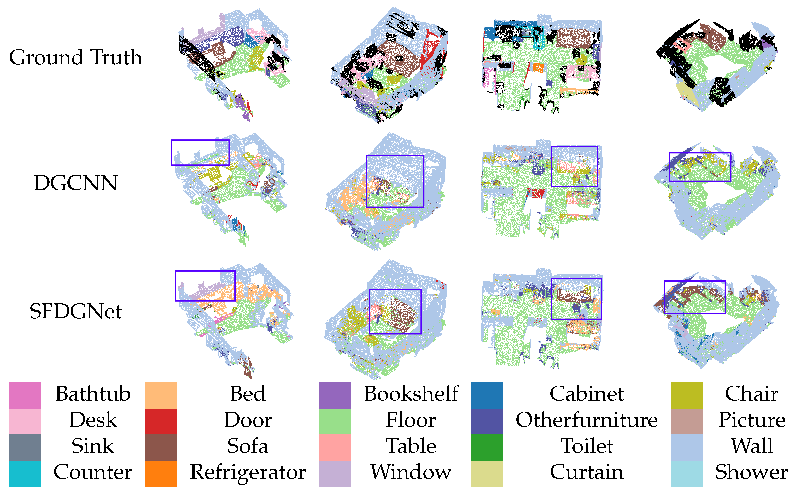
The experimental results in Table 9 and Figure 12 indicate that the proposed FS-DGCNN enhances the network’s sparse feature acquisition capability through sparse regularization algorithms, leading to improved segmentation performance across various test scenarios. Compared with the baseline model, MSE-DGCNN demonstrates significant mIoU improvement, confirming that the parallel construction of multi-range local neighborhood graphs, combined with SEConv modules, effectively extracts diverse neighborhood features and captures richer local point cloud characteristics. SFDGNet achieves marked improvements in both mIoU and sparsity metrics, demonstrating that the integrated approach of feature sparse regularization, parallel SEConv, and multi-neighborhood feature fusion not only enables deep feature extraction from different neighborhoods but also effectively emphasizes critical semantic features. However, its segmentation accuracy is significantly lower compared to the segmentation results of the network model on the S3DIS, primarily because the ScanNet contains more real-world noise, occlusions, complex environmental variations, and more severe class imbalance, which collectively impair the model’s ability to learn minority class features effectively.

6. Conclusions

The feature sparsity regularization method proposed in this study enables the network to progressively learn a sparse weight matrix during training and optimization, allowing the model to focus more on salient features and effectively improve its ability to select sparse features in point clouds. The proposed SFDGNet model extracts richer local edge features and enhances global feature representation through the integration of the SEConv module and the multi-neighborhood feature fusion strategy. The effectiveness and feasibility of both the feature sparsity regularization method and SFDGNet are thoroughly validated through comparative experiments and visual analyses. In future work, we will further investigate whether selecting larger combinations of neighborhood ranges can improve semantic segmentation performance, and how to optimize the algorithm and model architecture to reduce the spatiotemporal overhead introduced by larger neighborhood ranges, thereby providing theoretical support for robust semantic segmentation in open scenes.