Assessing Plant Water Status and Physiological Behaviour Using Multispectral Images from UAV in Merlot Vineyards in Central Spain

Abstract

Water status is a key determinant of physiological performance and vineyard productivity. However, its assessment through field measurements is time-consuming and labour-intensive. Remote sensing offers a fast and reliable alternative to traditional in situ methods for the monitoring of the water status in vineyards. This study aimed to assess the potential of high-resolution multispectral imagery acquired by UAVs to estimate the vine water status. The research was conducted over two growing seasons (2021 and 2022) in a commercial Merlot vineyard in Yepes (Toledo, Central Spain), under five irrigation regimes designed to generate a range of water statuses. UAV flights were performed at two times of day (09:00 and 12:00 solar time), coinciding with in-field measurements of physiological parameters. Stem water potential (SWP), chlorophyll content, and photosynthesis data were collected. The SWP consistently showed the strongest and most stable associations with vegetation indices (VIs) and the red spectral band at 12:00. A simple linear regression model using the NDVI explained up to 58% of the SWP variability regardless of the time of day or year. Multiple linear regression models incorporating the red and NIR bands yielded even higher predictive power (R² = 0.62). Stronger correlations were observed at 12:00, especially when combining data from both years, highlighting the importance of midday measurements in capturing water stress effects. These findings demonstrate the potential of UAV-based multispectral imagery as a non-destructive and scalable tool for the monitoring of the vine water status under field conditions.

1. Introduction

Wine grapes are one of Spain’s woodiest and most valuable crops [1]. Spain has the largest vineyard area in the world (949.565 ha in 2020), and the area of irrigated vineyards is increasing (from 33% in 2010 to more than 40% in 2020) [1]. The surface dedicated to vineyards for wine is around 1 million ha, with 41% under irrigation. Optimising water management has become increasingly crucial for wine producers due to the increasing water demand associated with the growing area of crop irrigation. The Food and Agriculture Organization (FAO) projected the global water demand for agriculture up to 2050 and identified that there would be an 11% increment from the 2006 baseline [2]. Furthermore, climate change events such as heatwaves are increasing in frequency, duration, and intensity in most of the key wine regions worldwide [3]. For this reason, irrigation will become an important tool to reduce the consequences of extreme events, as severe water stress can adversely affect the quality of berries, reducing the sugar and aroma levels, as well as lowering grape yields [4,5].

From this perspective, increasing the water use efficiency is highly relevant and is a key factor for irrigation sustainability [6]. During the vine’s growth cycle, the water needs vary significantly, and precise irrigation management can enhance the production quality and quantity. An adequate water supply is essential for vegetative development and cluster formation in the early stages. As the season progresses and the grapes ripen, controlled water deficits can concentrate sugars and phenolics, improving the wine quality [7].

The midday stem water potential (SWP) has been proposed as a significant physiological indicator of the plant water status for fruit trees and grapevines under irrigation [8,9,10]. Ref. [4] estimated different ranges of water status in vineyards based on the SWP for moderate to weak water deficits (−0.9 to −1.1 MPa), moderate to severe water deficits (−1.1 to −1.4 MPa), and severe water deficits (<−1.4). Nevertheless, these measurements are performed manually and are time-consuming and impossible to apply in commercial vineyards [11,12].

Water stress also affects other physiological parameters, such as net photosynthesis [13]. It also influences stomatal conductance, the chlorophyll content, and the leaf transpiration rate. The accumulated effect of these physiological parameters is evidenced in the leaf spectral response, which can be detected with remote sensing [14].

The plant water status could be assessed through remote sensing, proximal observations, and spectral analysis techniques [12]. Remote sensing methods based on spectral vegetation indices (VIs) and infrared thermometry are widely used for crop water stress detection because they are non-destructive, as well as the ease of obtaining information from a large area at once, reducing the labour and time requirements [13]. The efficient exploitation of all these techniques and observations towards accurately estimating the plant water status and mapping at the parcel scale arises as a challenging task [15].

Using unmanned aerial vehicles (UAVs) as platforms to obtain aerial imagery has several advantages over using satellites and other platforms [13]. UAVs, with lightweight, high-quality, calibrated geometric and radiometric sensors, allow users to obtain data with very high spatial (centimetric) and temporal resolutions, according to user needs. VIs, by combining spectral reflectance data from onboard sensors, have traditionally been used to monitor crops’ biochemical and biophysical attributes [16,17,18,19]. UAV imagery has been widely utilised in various agricultural applications; specifically, VIs have been used in plant vigour assessment, biomass production, disease detection, nitrogen content analysis, and crop water stress evaluation [17,20,21].

A few small-scale UAV studies with multispectral imagery have found that various VIs are significantly correlated with grapevine water stress through the SWP [22,23,24].

These studies have employed a variety of resources, including combinations of multispectral and thermal sensors [22,23], as well as complex classification techniques, such as random forests, support vector machines, and deep neural networks [24,25,26]. In particular, convolutional neural networks (CNNs) have demonstrated strong potential in crop stress detection and classification tasks by automatically extracting relevant spectral and spatial features from remote sensing data. However, these methods typically require extensive training data, the integration of multiple sensors, and significant computational resources [27,28,29,30,31].

While the advances in machine learning (ML) and deep learning (DL) approaches are well recognised [27], this study takes a different direction. Instead of focusing on high-complexity models, we assess whether a simple and operational approach—based solely on multispectral imagery from a single UAV-mounted camera—can reliably estimate a physiological parameter such as the stem water potential (SWP). The use of conventional regression techniques, including simple and multiple linear models, offers a more interpretable, accessible, and resource-efficient alternative, particularly suited for early-stage precision viticulture applications or scenarios with limited data and technical capacity.

To achieve this approach, high-resolution multispectral data from the vine canopy were analysed alongside physiological measurements, including the SWP, photosynthesis, and the chlorophyll content, which were recorded on nine days at 9:00 and 12:00 solar hours. The study was conducted over two growing seasons (2021 and 2022), with vines subjected to five irrigation treatments to generate a wide range of water status conditions and physiological behaviour. Additionally, the influence of the time of data acquisition (9:00 and 12:00 h) on the spectral responses was examined to determine whether it is a factor that should be considered in UAV-based water status monitoring.

2. Materials and Methods

2.1. Vineyard

This study was conducted on a commercial vineyard, Bodegas y viñedos Casa del Valle in Yepes (39°56′26.2″N, 3°42′49.7″W), Spain, at 699 masl during 2021 and 2022. The vineyard was planted in 2002 with cv. Merlot (Vitis vinifera L.) over SO4 rootstock (Selection Oppenheim 4) with a plantation frame of 2.6 × 1.1 m (3500 vines/ha). The plants had been trained in a double-cordon system and arranged on a trellis.

The area’s climate corresponds to a typical hot-summer Mediterranean climate. The region has an average daily temperature of 16 °C and average annual rainfall of 394 mm, mainly concentrated towards the end of autumn and the beginning of spring. Summers are characterised by a high atmospheric vapour demand derived from high temperatures (>40 °C max) and low relative humidity (RH). The air temperature and relative humidity were measured in-field using a portable weather station that provided minute data.

Temperature (°C), rainfall (mm), and reference evapotranspiration, ETo (mm) data were obtained from a meteorological station positioned 13 km from the experimental zone (Magán-Toledo, 505 masl, latitude 40°2′5.8″N and longitude 3°20′3.49″W, Huso UTM30 coord).

2.2. Irrigation Treatments

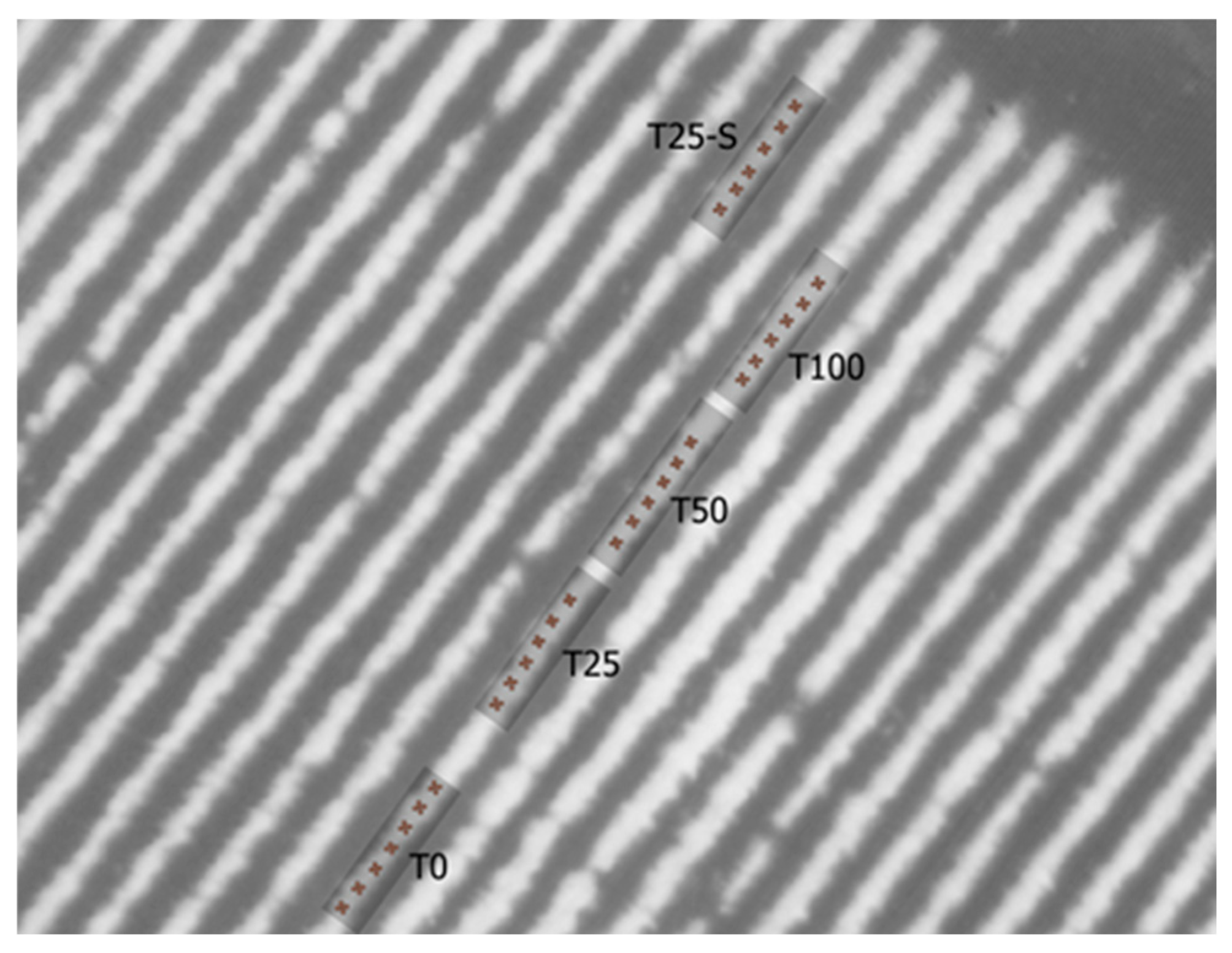
Five irrigation treatments were evaluated: four surface irrigation treatments, where different doses were achieved by modifying the distance between emitters, and one subsurface treatment corresponding to the standard irrigation practice carried out in the commercial vineyard. The water flow rate was identical for all treatments, at 2 L h⁻¹ per emitter. The different evaluated treatments are summarised below:

• T100: corresponds to 100% irrigation, with emitters every 0.25 m;
• T50: corresponds to 50% irrigation, with emitters every 0.50 m;
• T25: corresponds to 25% irrigation, with emitters every 1.0 m;
• T0: corresponds to 0% irrigation, with no emitters;
• T25-S: corresponds to the standard irrigation performed in the commercial vineyard, with sub-superficial emitters every 1.0 m (same dose as T25).

The study vines were located in two rows within a single vineyard plot. Each treatment consisted of six vines, totalling 30 vines across all treatments. Treatments T100, T50, T25, and T0 were arranged consecutively along a single row, with three border vines left between each treatment to minimise edge effects and avoid treatment interference. The T25-S treatment was spatially separated from the others and was located two rows away, as shown in Figure 1.

The irrigation periods varied between the years of study in terms of the duration and total quantities applied. In 2021, the irrigation season spanned from mid-May to the beginning of September. In 2022, the season was shorter, spanning from the end of June to the start of September, and the applied amount was also reduced. The irrigation doses for the different treatments were as follows:

• T100: 428 mm in 2021 (56%ETo) and 259 mm in 2022 (30%ETo);
• T50: 214 mm in 2021 (27%ETo) and 129 mm in 2022 (15%ETo);
• T25: 107 mm in 2021 (14%) and 65 mm in 2022 (8%ETo);
• T0: 0 mm in both seasons;
• T25-S: 107 mm in 2021 (14%) and 65 mm in 2022 (8%ETo).

Six vines were selected from each irrigation treatment to conduct the different experimental measurements.

2.3. Physiological and Agronomic Parameters

These measurements were conducted in six experimental vines for each irrigation treatment in both study seasons (2021 and 2022).

2.3.1. Stem Water Potential Measurements

The SWP (MPa) was measured at 9:00 and 12:00 solar time on 9 different dates: 25 June 2021, 5 July 2021, 20 July 2021, 30 July 2021, 19 August 2021, 30 June 2022, 15 July 2022, 5 August 2022, and 12 August 2022. Measurements were performed on healthy and shaded leaves from the inner part of the canopy, which was covered with a plastic bag with aluminium foil one hour before their use as a standardised method recommended to attain water status equilibrium between the stem and leaves. For this measurement, a Scholander-type pressure chamber was used (Soil Moisture Equipment Corp., Santa Barbara, CA, USA).

2.3.2. Photosynthesis

One fully expanded leaf per vine (6 vines/treatment, 30 leaves) was measured. The photosynthesis parameter was measured with a portable gas exchange system (CIRAS-2, PP Systems Ltd., Havervill, MA, USA) under the current air temperature and humidity, and the leaf cuvette (Automatic Leaf Universal Cuvette, PLC6) CO₂ concentration was set to ~400 ppm using a CO₂ cartridge.

2.3.3. Leaf Chlorophyll

The chlorophyll content in leaves (µmol chlorophyll/m² leaf area) was measured on the same dates and times as the SWP using a chlorophyll concentration meter (MC-100, Apogee Instruments Inc., Logan, UT, USA).

2.3.4. Vegetative Growth and Canopy Characteristics

Geometric measurements to describe canopy development were taken on 1 July 2021 and 20 June 2022; at this time, the vegetative growth had halted, and maximum vegetative expression had been achieved.

In each experimental vine, three points were selected to measure the canopy contour (using a flexible tape) and the distance between the highest and lowest leaves: the trunk and 40 cm on either side. At the same points, the canopy width was noted at three heights (80, 110, and 120 cm from the ground). From these measurements, the canopy height (H) and width (W) were derived, and the canopy volume and external canopy area were calculated as follows:

$$Canopy volume \left({\mathrm{m}}^3\right)=H\times W\times SV$$

(1)

$$External canopy area \left({\mathrm{m}}^2\right)=\left(2H+W\right)\times SV$$

(2)

where SV is the spacing between vines (m)

The leaf density was estimated as a gap percentage. A vine canopy photo of each experimental vine with a red blanket at the back was taken to delimit it. Using the ImageJ software version 1.53e (Wayne Rasband, Bethesda, MD, USA), the photos were binarised to calculate the gaps in the canopy.

Finally, the pruning weight was taken on 2 February 2022 (corresponding to season 2021) and 5 February 2023 (corresponding to season 2022).

2.3.5. Production and Quality

Experimental vines were harvested by hand according to the commercial vineyard manager’s decision concerning optimal productive characteristics. The selected dates were 20 August 2021 and 16 August 2022. During the harvest, we randomly selected 150–200 berries from each vine, which were packaged, ragged, and stored in a cooler.

The selected berries were taken to the laboratory, counted, and weighed immediately. Then, they were processed to determine the °Brix.

2.4. Multispectral Images and VIs

Aerial images were acquired employing an unmanned aerial vehicle (UAV) (model eBee, AgEagle Aerial Systems Inc., Wichita, KS, USA), a commercial fixed-wing platform equipped with a Parrot Sequoia (Parrot© SA, 2017, Paris, France) multispectral sensor. Flights were carried out at 120 m altitude on the same dates and times at which the SWP measurements were carried out (9:00 and 12:00 solar time). The different high-resolution imagery consisted of RGB images (3 cm/pixel) and multiband images (12 cm/pixel) that included the green (495–570 nm), red (620–750 nm), red edge (670–760 nm), and near-infrared (NIR) (780–2500 nm) bands. These bands include regions in the visible spectrum (green and red) and infrared spectrum (red edge and NIR).

UAV image acquisition was conducted on five dates during 2021 and four dates in 2022. On each date, two flights were performed—one at 09:00 and one at 12:00. This resulted in a total of 10 UAV flights in 2021 and 8 in 2022. All flights were carried out under clear sky conditions, and consistent flight parameters were maintained across dates to ensure data comparability.

UAV flights were conducted at a speed of 50 km/h, lateral overlap of 70%, and longitudinal overlap of 70% to ensure sufficient photogrammetric reconstruction. All missions were carried out using an RTK-enabled system, which provided centimetre-level spatial accuracy.

Before the flight, a dedicated Sequoia equipment calibration plate was applied with the Parrot Sequoia camera to normalise the local lighting. Image processing was performed using Pix4Dmapper, including radiometric correction, band alignment, orthomosaic generation, and reflectance map calculation.

After image processing by Unmanned Technical Works (UTW), band pixel information was extracted using the QGIS software (3.22.13, Biolowieza, Poland). Given the high spatial resolution (12 cm/pixel) of the multiband images, only pure canopy pixels were selected to minimise soil interference. To ensure representative measurements, five pixels were sampled from the centremost area of each vine, and their mean reflectance value was used. This sampling strategy was not arbitrary but intentionally designed to minimise the influence of mixed pixels, edge effects, and background noise. The five central canopy pixels were selected based on GPS-referenced plant locations, allowing us to precisely identify and extract pure vegetation pixels from each target vine. This ensured consistent and spatially accurate reflectance values across the dataset, which was particularly important given the high resolution of the imagery and the limited sample size.

The mean reflectance of these five pixels was then calculated to obtain a representative value for each plant. These reflectance values were loaded into a spreadsheet where VIs were calculated. Based on the available bands and cited literature, the following indices were calculated: the normalised difference vegetation index (NDVI), the renormalised difference vegetation index (RDVI), the transformed chlorophyll absorption ratio (TCARI), the optimised soil adjusted vegetation index (OSAVI), the normalised difference red-edge index (NDRE), and the green normalised difference vegetation index (GNDVI). Their formulas are presented in

Table 1. Formulas and references for the vegetation indices (VIs) used in this study.

Index	Formula	Reference
NDVI	$NDVI={\displaystyle \frac{R_{NIR}-R_{Red}}{R_{NIR}+R_{Red}}}$	[32]
RDVI	$RDVI={\displaystyle \frac{R_{NIR}-R_{Red}}{\sqrt{R_{NIR}+R_{Red}}}}$	[33]
TCARI	$TCARI=3\times [\left(R_{Red Edge}-R_{Red}\right)-0.2\times \left(R_{Red Edge}-R_{Green}\right)\times \left({\displaystyle \frac{R_{Red Edge}}{R_{Red}}}\right)]$	[34]
OSAVI	$OSAVI=\left(1+0.16\right)\times \left(R_{NIR}-R_{Red}\right)/\left(R_{NIR}+R_{Red}+0.16\right)$	[35]
NDRE	$NDRE={\displaystyle \frac{R_{NIR}-R_{Red Edge}}{R_{NIR}+R_{Red Edge}}}$	[36]
GNDVI	$GDVI={\displaystyle \frac{R_{NIR}-R_{Green}}{R_{NIR}+R_{Green}}}$	[37]

, where R_BAND is the reflectance value for the designated band wavelength.

2.5. Statistical Analysis

Statistical analyses were conducted using the Infostat software (version 1.5, Universidad Nacional de Córdoba, Córdoba, Argentina), Statgraphics 19 software (Statgraphics Technologies, Inc., The Plains, VA, USA), and RStudio version 2024.09.0 Build 375.

The dataset was based on five irrigation treatments applied to a total of 30 plants, with six vines per treatment. To reduce the within-treatment variability and enhance the reliability of the statistical comparisons, the data were averaged per treatment. Measurements were conducted on five dates in 2021 and four in 2022, at two time points each day (09:00 and 12:00). This resulted in a final dataset composed of mean values for the five treatments, collected across nine measurement dates and two time points per day, yielding a total of 90 observations (5 treatments × 9 dates × 2 time points).

To assess differences among irrigation treatments in terms of the physiological parameters and reflectance values of the spectral bands and vegetation indices (VIs), an analysis of variance (ANOVA) was performed using the Infostat software. Post hoc comparisons were conducted using Fisher’s least significant difference (LSD) test, with the significance level set at p < 0.05.

The normality of the physiological variables, spectral band reflectance, and VIs was evaluated using the Shapiro–Wilk test. Pearson or Spearman correlations were selected based on the Shapiro–Wilk test results. This correlation allowed for the identification of relationships between the physiological parameters and both the spectral bands and VIs.

The spectral bands and VIs showing the strongest and most consistent correlations (r > 0.5) across the four different evaluated scenarios (09:00 in 2021, 9:00 in 2022, 12:00 in 2021, and 12:00 in 2022) were selected for further analysis. Simple and multiple linear regression models were developed to estimate the physiological parameter of interest. The models were developed using a 70/30 train–test split in RStudio version 2024.09.0 Build 375.

A simple linear regression was performed using the VIs that showed the strongest correlations with the physiological parameter.

A multiple linear regression model was initially developed using four spectral bands—green, red, red edge, and NIR—as predictor variables. Each band’s contribution was evaluated based on statistical significance (p < 0.05), and those not significantly contributing to the model were progressively removed. In addition, multicollinearity among the spectral bands was assessed using variance inflation factors (VIFs). Model performance was evaluated using multiple error and fit metrics, including the coefficient of determination (R²), mean absolute error (MAE), root mean square error (RMSE), and mean absolute percentage error (MAPE).

The normality of model residuals was assessed using the Shapiro–Wilk test in RStudio. In addition, model assumptions were evaluated through the visual inspection of the residual vs. fitted value plots to assess homoscedasticity, and Q–Q plots were used to examine the normality of residuals.

3. Results

3.1. Climatic Conditions

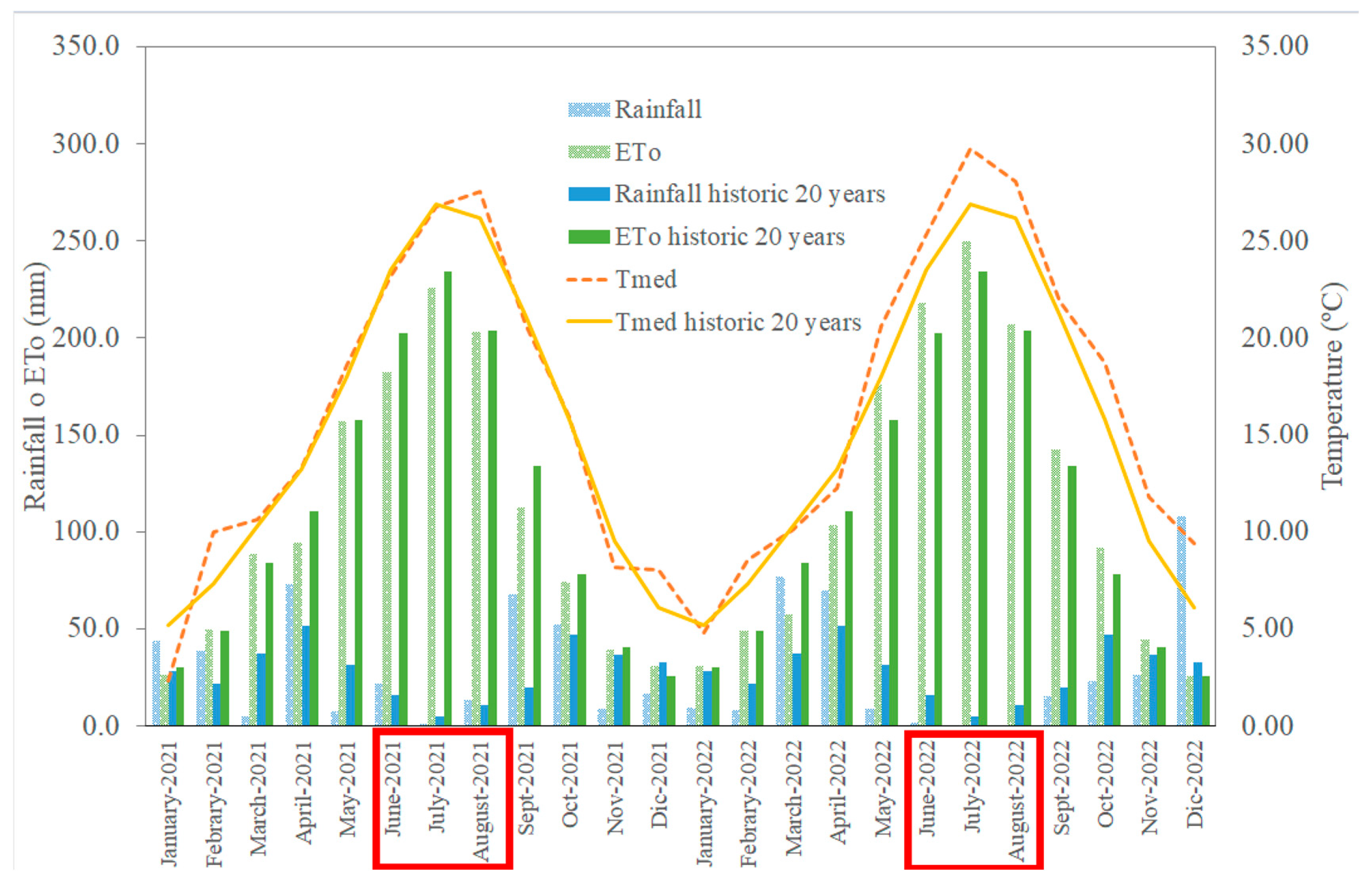
The meteorological conditions are presented in Figure 2. The graph shows the rainfall, evapotranspiration (ETo), and mean temperature (Tmed) for 2021 and 2022 compared to a 20-year historical series. The red boxes highlight the months during which the study was conducted.

The annual rainfall (349 mm) was similar between 2021 and 2022. The rainfall was 167 and 173 mm from January to May in 2021 and 2022, respectively. During the experimental period (June–August), the precipitation was 36 and 2 mm in 2021 and 2022. Differences in the annual ETo were observed, with values of 1284 and 1395 mm in 2021 and 2022.

The conditions were highly evaporative during the experimental period (June–August), with high cumulative ETo (390 and 441 mm in 2021 and 2022, respectively). August was the hottest month in 2021 (Tmean 27.5 °C), and July was the hottest in 2022 (Tmean 29.8 °C). The ETo in 2022 was higher than in 2021, likely due to the elevated temperatures observed that year. In 2022, the temperatures were higher, especially during the summer and autumn months, which led to increased evapotranspiration. These differences highlight a warmer 2022 compared to 2021, which correlated with higher ETo values and more rainfall during specific months.

Table 2. Air temperature (Ta), relative humidity (RH), and vapour pressure deficit (VPD) at 9:00 and 12:00 and daily reference evapotranspiration (ETo) within the canopy during the days of the UAV flight.

	9:00			12:00
	Ta (°C)	RH (%)	VPD (KPa)	Ta (°C)	RH (%)	VPD (KPa)	ETo (mm/day)
25 June 2021	27.4	43.9	2.1	33.5	29.8	3.6	6.6
5 July 2021	28.2	42.8	2.2	34.0	30.8	3.7	8.2
20 July 2021	28.8	39.6	2.4	35.9	19.8	4.7	7.9
30 July 2021	28.3	34.1	2.5	33.6	12.7	4.5	9.1
AVERAGE 2021	28.3	40.3	2.3	34.0	23.2	4.1	7.6
30 June 2022	27.5	28.2	2.6	30.0	23.1	3.3	7.0
15 July 2022	35.2	22.6	4.4	40.2	15.4	6.3	8.1
5 August 2022	29.1	37.7	2.5	36.6	18.4	5.0	7.3
12 August 2022	29.3	31.0	2.8	36.6	21.2	4.8	6.3
AVERAGE 2022	30.3	29.8	3.1	35.9	19.5	4.9	7.2

shows the air temperature (Ta), relative humidity (RH), and vapour pressure deficit (VPD) within the canopy at the two times of day at which the measurements were obtained. The Ta annual average at 9:00 and 12:00 in 2022 was 2 °C higher than in 2021. The RH decreased by 26% at 9:00 and 16% at 12:00 h in 2022 compared to the same hours in 2021. In 2022, the annual average VPD was higher than in 2021. The highest VPD value was recorded on 15 July 2022. The lowest ETo occurred at the beginning of the season for both years (25 June 2021 and 30 June 2022) and the highest on 30 July 2021 and 15 July 2022.

3.2. Physiological and Agronomic Parameters

3.2.1. Physiological Measurements

Table 3. Annual averages of physiological parameters (SWP, chlorophyll, and photosynthesis) for two campaigns (2021 and 2022) under five irrigation treatments: T100 (reference treatment), T50 (50% of reference treatment), T25 (25% of reference treatment), T0 (rainfed), and T25-S (25% of reference treatment subsurface).

		9:00					12:00
Year	Parameter	T100	T50	T25	T0	T25-S	T100	T50	T25	T0	T25-S
2021	SWP (MPa)	−0.6 a	−0.6 a	−0.8 b	−0.9 b	−0.8 b	−0.8 a	−0.9 ab	−1.0 bc	−1.1 c	−1.0 bc
	Photosynthesis (μmol/m2s)	9.3 a	7.7 b	4.6 c	4.5 c	5.3 c	5.9 a	3.3 b	1.5 cd	1.0 d	2.3 bc
	Chlorophyll (µmol/m2)	22.6	21.1	18.4	20.1	18.7	23.1	22.9	20.3	20.8	19.2
2022	SWP (MPa)	−1.1 a	−1.3 b	−1.5 cd	−1.5 d	−1.3 bc	−1.3 a	−1.4 ab	−1.5 bc	−1.6 c	−1.4 ab
	Photosynthesis (μmol/m2s)	3.9 a	2.2 ab	2.2 ab	1.3 b	2.2 ab	4.2 a	2.1 b	2.0 b	1.3 b	1.5 b
	Chlorophyll (µmol/m2)	16.6	16.9	15.7	15.0	16.6	17.5	16.5	16.5	15.5	16.5

Means with different letters indicate significant differences at p < 0.05 between treatments at each measured hour.

shows the annual mean values of the physiological parameters measured for each irrigation treatment. The irrigation treatments significantly modified the SWP across both measurement times and study years. In 2021, the values ranged from −0.6 MPa to −1.1 MPa. At 9:00, the rainfed treatment (T0) recorded a more negative SWP (−0.9 MPa) than the irrigated treatments T50 and T100. A similar trend was observed at 12:00, with T0 again showing the lowest seasonal value (−1.1 MPa). According to the daily data (

Table A1. Mean and standard deviation (SD) of stem water potential (MPa) measured at two hours per day and over two campaigns (2021 and 2022) under five irrigation treatments: T100 (reference treatment), T50 (50% of reference treatment), T25 (25% of reference treatment), T0 (rainfed), and T25-S (25% of reference treatment subsurface).

		9:00					12:00
Day	Statistic	T100	T50	T25	T0	T25-S	T100	T50	T25	T0	T25-S
25 June 2021	Mean	−0.5 a	−0.5 a	−0.6 b	−0.6 b	−0.6 b	−0.6 a	−0.7 b	−0.8 c	−1.0 d	−0.8 c
	SD	0.02	0.01	0.04	0.03	0.04	0.02	0.03	0.03	0.03	0.03
5 July 2021	Mean	−0.4 a	−0.5 a	−0.6 b	−0.8 c	−0.7 b	−0.6 a	−0.8 b	−0.9 c	−1.1 d	−0.9 b
	SD	0.02	0.02	0.04	0.04	0.03	0.04	0.03	0.05	0.04	0.05
20 July 2021	Mean	−0.5 a	−0.6 ab	−0.6 bc	−0.8 d	−0.7 cd	−0.7 a	−0.8 b	−0.9 bc	−1.1 d	−1.0 c
	SD	0.05	0.01	0.04	0.07	0.03	0.07	0.04	0.04	0.04	0.02
30 July 2021	Mean	−0.7 a	−0.8 a	−1.0 b	−1.2 c	−1.1 c	−1.2	−1.2	−1.2	−1.3	−1.3
	SD	0.07	0.05	0.03	0.08	0.04	0.15	0.05	0.20	0.19	0.11
19 August 2021	Mean	−0.7 a	−0.8 b	−1.1 b	−1.2 b	−1.2 b	−1.33 a	−1.37 b	−1.7 c	−1.8 d	−1.4 b
	SD	0.11	0.12	0.01	0.10	0.13	0.12	0.20	0.18	0.18	0.18
30 June 2022	Mean	−1.2 c	−1.2 bc	−1.2 bc	−1.1 ab	−1.1 a	−1.1	−1.11	−1.0	−1.0	−1.1
	SD	0.10	0.11	0.14	0.09	0.02	0.06	0.02	0.03	0.02	0.02
15 July 2022	Mean	−1.4	−1.5	−1.4	−1.7	−1.3	−1.6	−1.4	−1.5	−1.6	−1.4
	SD	0.20	0.29	0.19	0.39	0.18	0.33	0.19	0.21	0.28	0.21
5 August 2022	Mean	−1.0 a	−1.3 b	−1.8 d	−1.6 c	−1.6 c	−1.4 a	−1.6 b	−1.8 c	−1.8 c	−1.7 bc
	SD	0.07	0.10	0.10	0.28	0.06	0.08	0.11	0.19	0.19	0.13
12 August 2022	Mean	−0.8 a	−1.1 b	−1.5 d	−1.6 d	−1.2 c	−1.1 a	−1.3 b	−1.7 d	−1.8 d	−1.4 c
	SD	0.07	0.06	0.04	0.21	0.12	0.05	0.09	0.13	0.16	0.17

Means with different letters indicate significant differences at p < 0.05 between treatments at each measured hour.

), this treatment reached its minimum value of −1.8 MPa on 19 August 2021 at 12:00. Overall, the midday mean values suggest mild water stress in T100 and T50 and moderate stress in the remaining treatments.

In 2022, the values showed lower means at both measurement times compared to 2021. The values ranged from −1.1 to −1.6 MPa. At 9:00, significant differences were observed between treatments, particularly between T0 and T100. A similar situation was found at 12:00, where T0 recorded the lowest SWP value among all treatments (−1.6 MPa).

A similar pattern was observed for photosynthesis, which was also influenced by the irrigation treatments. In 2021, the range of photosynthetic values varied from 1.0 to 9.3 μmol/m2s. The T0 treatment showed the lowest values at both 9:00 and 12:00 (4.5 and 1.0 μmol/m2s, respectively). The mean values at 12:00 showed a clear decrease compared to those recorded at 9:00 across all treatments. In 2022, the average photosynthetic rates were lower than those observed in 2021, especially at 9:00.

No significant differences in chlorophyll content were found among the irrigation treatments. Nevertheless, as observed for the SWP and photosynthesis, the mean chlorophyll values in 2022 were consistently lower than those recorded in 2021 at both measurement times (9:00 and 12:00).

The daily data for each physiological parameter are presented in Appendix A (Table A1,

Table A2. Photosynthesis (μmol/m²s) measured at two hours per day and over two campaigns (2021 and 2022) under five irrigation treatments: T100 (reference treatment), T50 (50% of reference treatment), T25 (25% of reference treatment), T0 (rainfed), and T25-S (25% of reference treatment, subsurface irrigation).

		9:00					12:00
Day	Statistic	T100	T50	T25	T0	T25-S	T100	T50	T25	T0	T25-S
25 June 2021	Mean	7.1	5.1	3.7	3.3	6.4	8.0 a	4.3 b	1.0 bc	0.9 bc	0.6 c
	SD	3.94	3.91	3.03	0.54	2.96	2.66	1.73	2.30	1.86	2.73
5 July 2021	Mean	6.8 a	7.6 a	3.3 b	5.4 ab	5.9 ab	8.0 a	5.3 b	1.3 c	1.0 c	4.7 b
	SD	2.40	2.67	0.69	1.07	1.69	1.84	3.02	0.45	0.83	0.36
20 July 2021	Mean	9.9 a	5.7 b	4.9 b	4.5 b	5.5 b	1.7	−0.4	−0.1	−0.6	−0.3
	SD	1.37	3.05	1.21	0.97	0.96	1.35	0.80	0.43	1.19	1.62
30 July 2021	Mean	12.1 a	10.5 a	6.3 b	3.9 c	4.7 bc	7.3 a	3.8 b	2.9 b	0.8 c	2.8 b
	SD	1.78	0.75	2.11	1.85	0.62	1.20	0.50	0.72	1.52	1.07
19 August 2021	Mean	10.8 a	9.7 b	4.4 c	4.2 cd	3.6 d	6.6 a	4.6 b	1.4 c	1.3 c	3.2 b
	SD	0.59	0.56	0.28	0.55	0.51	0.12	0.20	0.18	0.19	0.18
30 June 2022	Mean	−2.1	−2.7	−1.4	−2.5	−2.8	3.5	2.4	4.9	1.5	1.6
	SD	0.96	0.67	1.98	0.25	0.38	1.97	0.86	0.85	3.24	1.54
5 August 2022	Mean	5.2 a	2.2 b	2.1 b	1.9 b	3.3 ab	6.1 a	0.8 b	1.0 b	0.8 b	1.2 b
	SD	1.86	0.29	1.21	0.65	1.60	2.46	0.87	0.39	1.35	0.18
12 August 2022	Mean	3.8 a	3.3 a	2.0 b	1.7 b	3.2 a	2.2	1.5	1.2	1.2	1.5
	SD	0.73	0.82	0.67	0.50	0.89	0.81	0.42	0.38	0.45	1.01

Means with different letters indicate significant differences at p < 0.05 between treatments at each measured hour.

and

Table A3. Chlorophyll (µmol/m²) measured at two hours per day and over two campaigns (2021 and 2022) under five irrigation treatments: T100 (reference treatment), T50 (50% of reference treatment), T25 (25% of reference treatment), T0 (rainfed), and T25-S (25% of reference treatment, subsurface irrigation).

		9:00					12:00
Day	Statistic	T100	T50	T25	T0	T25-S	T100	T50	T25	T0	T25-S
25 June 2021	Mean	16.3	16.2	19.1	17.4	16.4	20.3	19.9	18.8	18.5	17.3
	SD	1.91	1.56	1.37	4.16	1.89	3.47	3.59	1.95	4.83	1.16
5 July 2021	Mean	20.9	20.7	17.5	20.7	20.5	23.7	20.3	21.5	21.1	19.0
	SD	5.02	2.02	4.11	2.71	3.37	2.40	2.02	3.11	5.12	1.69
20 July 2021	Mean	21.2 a	18.5 ab	14.3 b	17.7 ab	16.2 b	23.1	23.7	22.2	22.5	24.2
	SD	3.85	2.85	2.85	2.21	2.15	4.96	1.73	3.18	4.33	3.71
30 July 2021	Mean	28.8	26.4	22.8	24.6	22.9	24.1 ab	27.1 a	20.9 bc	22.5 abc	17.6 c
	SD	6.13	2.29	1.65	2.61	1.10	5.16	3.64	2.33	3.46	3.51
19 August 2021	Mean	26.2	23.6	18.4	19.8	17.6	24.4 a	23.5 a	17.8 b	19.2 b	17.8 b
	SD	1.57	6.65	3.44	3.58	4.59	20.3	19.9	18.8	18.5	17.3
30 June 2022	Mean	16.2	17.1	16.8	16.2	17.0	18.1	16.9	18.5	17.7	17.6
	SD	1.28	1.50	1.55	3.36	1.66	1.13	2.69	0.54	2.09	1.77
15 July 2022	Mean	15.1	17.1	17.3	15.4	17.3	16.9	18.0	18.0	17.9	17.8
	SD	2.22	2.44	2.53	1.90	1.21	1.93	1.66	3.22	1.46	1.18
5 August 2022	Mean	18.4 a	16.2 b	14.2 b	14.6 b	15.7 b	18.9 a	14.5 b	15.1 b	13.4 b	15.5 b
	SD	2.30	1.35	0.50	2.74	1.13	1.50	1.96	2.29	1.79	0.89
12 August 2022	Mean	16.6 a	17.2 a	14.8 b	13.9 b	16.3 a	16.2 ab	16.6 a	14.5 bc	12.9 c	15.0 ab
	SD	0.93	1.30	1.24	0.86	0.68	0.86	1.50	1.90	0.78	1.96

Means with different letters indicate significant differences at p < 0.05 between treatments at each measured hour.

).

3.2.2. Vegetative Growth, Production, and Quality

The irrigation treatments significantly modified the vegetative growth, specifically regarding the external canopy area and volume (

Table 4. Vegetative growth, productive, and quality parameters of the experimental vines—external canopy area; canopy volume and gaps; and pruning weight, berry weight, and sugar content (°Brix)—over two campaigns (2021 and 2022) under five irrigation treatments: T100 (reference treatment), T50 (50% of reference treatment), T25 (25% of reference treatment), T0 (rainfed), and T25-S (25% of reference treatment, irrigation subsurface).

	2021					2022
Parameter	T100	T50	T25	T0	T25-S	T100	T50	T25	T0	T25-S
External canopy area (m2)	2.3 a	2.3 a	2.2 ab	1.9 b	2.4 a	3.2	3.2	3.2	2.9	3.1
Canopy volume (m3)	0.6 a	0.5 a	0.5 ab	0.4 b	0.6 a	1.0	1.1	1.1	1.0	1.0
Canopy gaps (%)	35.0	35.8	33.7	32.3	36.8	23.3	25.4	21.5	23.5	25.6
Pruning weight (g/plant)	250.0	150.0	212.5	212.5	225.0	260.0	176.7	178.3	141.7	261.7
Berry weight (g)	1.1 a	0.9 b	0.8 c	0.7 c	0.9 b	0.5 a	0.5 a	0.4 b	0.3 b	0.5 a
°Brix	28.5	29.1	30.0	32.1	31.8	23.1 cd	22.3 d	24.7 ab	25.7 a	24.1 bc

Means with different letters indicate significant differences at p < 0.05 between treatments at each measured hour.

). Significant differences between the irrigation treatments were mainly observed in 2021. The external canopy area of the most irrigated treatment (T100) was 23% larger than that of the least irrigated treatment (T0). A similar situation was observed for the canopy volume: that of T100 was 53% higher than that of T0.

In 2022, the average values of all parameters of vegetative growth increased for all treatments, except for the gap percentage, which was lower in 2021. This indicates greater vegetative development in 2022. The volume increased by over 100% compared to 2021 for all treatments.

The irrigation treatment did not significantly affect the weight of pruned wood, and small differences were observed between years.

The berry weight and °Brix were the productive and quality parameters that were significantly modified by the irrigation treatments (Table 4). The weight of berries was influenced by the year. In 2022, the berry weight decreased by 50% across all treatments. The irrigation treatments T0 and T25 showed significant differences compared to T100, T50, and T25-S.

T100 and T50 presented significantly lower °Brix values than T0, T25, and T25-S in 2022.

3.3. Multispectral Images and Vegetation Indices

Table 5. Annual average values of multispectral bands (green, red, red edge, and NIR) and VIs (NDVI, RDVI, TCARI, OSAVI, NDRE, and GNDVI) for two campaigns (2021 and 2022) under five irrigation treatments: T100 (reference treatment), T50 (50% of reference treatment), T25 (25% of reference treatment), T0 (rainfed), and T25-S (25% of reference treatment subsurface).

		9:00					12:00
	Band	T100	T50	T25	T0	T25-S	T100	T50	T25	T0	T25-S
	Green	0.07	0.07	0.08	0.07	0.08	0.07 b	0.07 b	0.07 a	0.07 b	0.07 a
	Red	0.05 b	0.05 b	0.06 a	0.06 a	0.06 a	0.06 c	0.06 bc	0.06 a	0.06 ab	0.07 a
Average	Red Edge	0.28	0.23	0.28	0.24	0.26	0.26 ab	0.25 bc	0.27 a	0.25 c	0.25 bc
2021	NIR	0.47 a	0.39 bc	0.45 ab	0.38 c	0.42 abc	0.44 a	0.40 bc	0.41 ab	0.37 c	0.40 bc
	Green	0.11 bc	0.10 c	0.12 a	0.11 ab	0.10 c	0.10	0.09	0.10	0.10	0.10
	Red	0.09 bc	0.08 c	0.10 a	0.09 ab	0.08 c	0.08	0.07	0.08	0.08	0.07
Average	Red Edge	0.36 abc	0.35 c	0.38 a	0.47 ab	0.35 bc	0.28	0.27	0.27	0.27	0.28
2022	NIR	0.51	0.49	0.51	0.51	0.52	0.41	0.39	0.38	0.39	0.40
	VI
	NDVI	0.81 a	0.77 b	0.77 b	0.73 c	0.75 bc	0.77 a	0.74 b	0.73 bc	0.71 c	0.72 c
	RDVI	0.58 a	0.50 bc	0.55 ab	0.48 c	0.52 bc	0.54 a	0.50 bc	0.51 b	0.47 c	0.49 bc
	TCARI	−0.02 b	0.05 ab	0.04 ab	0.09 a	0.08 a	0.06 c	0.09 bc	0.10 b	0.12 ab	0.14 a
Average	OSAVI	0.71 a	0.65 bc	0.68 ab	0.62 c	0.65 bc	0.68 a	0.64 b	0.64 b	0.61 c	0.62 bc
2021	NDRE	0.26 a	0.25 a	0.23 b	0.22 b	0.23 b	0.25 a	0.23 b	0.21 c	0.20 c	0.23 b
	GNDVI	0.73 a	0.69 b	0.69 b	0.67 b	0.68 b	0.73 a	0.70 b	0.70 b	0.69 b	0.69 b
	NDVI	0.71 ab	0.71 ab	0.67 c	0.69 bc	0.73 a	0.67 ab	0.68 ab	0.66 b	0.66 b	0.71 a
	RDVI	0.55 ab	0.53 b	0.52 b	0.53 b	0.57 a	0.47 ab	0.47 ab	0.45 b	0.46 ab	0.49 a
	TCARI	0.17	0.12	0.22	0.18	0.15	0.19	0.16	0.19	0.18	0.17
Average	OSAVI	0.65 ab	0.64 abc	0.61 c	0.63 bc	0.67 a	0.59	0.59	0.57	0.58	0.61
2022	NDRE	0.18 b	0.17 c	0.15 d	0.16 cd	0.19 a	0.19	0.18	0.18	0.18	0.19
	GNDVI	0.66 a	0.65 ab	0.63 b	0.63 b	0.67 a	0.61	0.61	0.59	0.6	0.62

Means with different letters indicate significant differences at p < 0.05 between treatments at each measured hour.

presents the annual average values of the individual spectral bands and VIs for each measurement time and year. In 2021, the irrigation treatments showed significant differences from the four spectral bands at 12:00. However, no significant differences were observed for the green and NIR bands at 9:00. In 2022, the irrigation treatments showed significant differences at 9:00 for the green, red, and red edge bands. No significant differences were found between the irrigation treatments for any of the studied bands at 12:00.

Regarding the VIs, in 2021, the different irrigation treatments showed significant differences at both 9:00 and 12:00. In 2022, the RDVI at 9:00 and the TCARI, OSAVI, NDRE, and GNDVI at 12:00 did not show significant differences between the treatments.

The daily data for the VIs and spectral bands are presented in Appendix A (

Table A4. Different bands calculated from a high-resolution (12 cm/pixel) multispectral sensor mounted onboard a UAV at two solar times (09:00 and 12:00) in 2021 under five irrigation treatments in a commercial vineyard in Central Spain (Yepes, Toledo).

		9:00					12:00
	Band	T100	T50	T25	T0	T25-S	T100	T50	T25	T0	T25-S
25 June 2021	Green	0.10 a	0.09 c	0.09 bc	0.09 bc	0.10 ab	0.06 b	0.06 b	0.06 b	0.06 b	0.07 a
	Red	0.07	0.06	0.06	0.07	0.07	0.05 c	0.05 c	0.05 c	0.05 b	0.06 a
	Red Edge	0.42 a	0.36 bc	0.39 b	0.36 c	0.38 bc	0.25 b	0.26 ab	0.27 a	0.25 b	0.25 b
	NIR	0.67 a	0.59 bc	0.61 b	0.57 c	0.62 b	0.41	0.4	0.42	0.39	0.41
5 July 2021	Green	0.06	0.06	0.07	0.06	0.06	0.07 bc	0.07 c	0.07 a	0.07 c	0.07 ab
	Red	0.04	0.04	0.05	0.05	0.04	0.05 c	0.05 bc	0.06 a	0.06 a	0.06 ab
	Red Edge	0.25 b	0.22 c	0.28 a	0.25 b	0.23 c	0.28 a	0.26 c	0.27 ab	0.25 c	0.27 bc
	NIR	0.41 b	0.35 c	0.45 a	0.39 b	0.35 c	0.46 a	0.42 b	0.43 b	0.39 c	0.42 bc
20 July 2021	Green	0.06 bc	0.06 c	0.07 ab	0.06 c	0.08 a	0.08	0.08	0.08	0.08	0.08
	Red	0.04 b	0.04 b	0.05 a	0.05 a	0.05 a	0.06 c	0.06 c	0.07 b	0.07 b	0.07 a
	Red Edge	0.22 a	0.18 b	0.23 a	0.18 b	0.22 a	0.30 a	0.28 cd	0.28 bc	0.27 d	0.29 b
	NIR	0.41 a	0.31 b	0.37 a	0.29 b	0.37 a	0.52 a	0.45 c	0.44 c	0.40 d	0.47 b
30 July 2021	Green	0.07 bc	0.07 c	0.08 b	0.07 c	0.08 a	0.06	0.06	0.07	0.06	0.07
	Red	0.05 b	0.05 b	0.06 a	0.06 a	0.06 a	0.06 b	0.07 a	0.07 a	0.06 b	0.07 a
	Red Edge	0.29 a	0.22 c	0.25 b	0.21 c	0.27 ab	0.25 b	0.24 b	0.27 a	0.26 ab	0.24 b
	NIR	0.49 a	0.37 c	0.39 bc	0.32 d	0.42 b	0.43 a	0.39 bc	0.42 a	0.40 ab	0.38 c
19 August 2021	Green	0.06 c	0.08 b	0.10 a	0.08 b	0.08 b	0.06 c	0.07 bc	0.07 ab	0.07 c	0.08 a
	Red	0.05	0.06	0.07	0.06	0.07	0.05 c	0.06 bc	0.07 ab	0.06 b	0.07 a
	Red Edge	0.22 b	0.19 c	0.27 a	0.21 bc	0.22 b	0.23 a	0.21 b	0.23 a	0.21 b	0.21 b
	NIR	0.37 b	0.32 c	0.43 a	0.34 c	0.33 c	0.38 a	0.32 b	0.34 b	0.30 c	0.33 b

Means with different letters indicate significant differences at p < 0.05 between treatments at each measured hour.

,

Table A5. Different bands calculated from a high-resolution (12 cm/pixel) multispectral sensor mounted onboard a UAV at two solar times (09:00 and 12:00) in 2022 under five irrigation treatments in a commercial vineyard in Central Spain (Yepes, Toledo).

		9:00					12:00
	Band	T100	T50	T25	T0	T25-S	T100	T50	T25	T0	T25-S
30 June 2022	Green	0.09 a	0.08 b	0.09 a	0.09 a	0.09 a	0.09 a	0.08 d	0.08 cd	0.09 ab	0.09 bc
	Red	0.07 ab	0.06 c	0.07 a	0.06 bc	0.06 bc	0.06 a	0.05 c	0.06 bc	0.06 bc	0.06 b
	Red Edge	0.36	0.34	0.36	0.35	0.35	0.3	0.29	0.29	0.29	0.29
	NIR	0.52	0.49	0.52	0.52	0.51	0.45	0.44	0.43	0.44	0.43
15 July 2022	Green	0.11 b	0.10 bc	0.11 a	0.11 ab	0.10 c	0.10 a	0.09 b	0.09 b	0.09 b	0.09 b
	Red	0.09 b	0.08 b	0.10 a	0.09 b	0.08 b	0.07 ab	0.07 c	0.07 a	0.07 bc	0.06 c
	Red Edge	0.35	0.36	0.37	0.37	0.34	0.28	0.28	0.27	0.28	0.26
	NIR	0.49	0.49	0.5	0.52	0.43	0.40 a	0.38 ab	0.37 b	0.38 ab	0.39 a
5 August 2022	Green	0.11 b	0.12 b	0.14 a	0.14 a	0.11 b	0.11 ab	0.10 bc	0.10 abc	0.10 c	0.11 a
	Red	0.10 b	0.10 b	0.12 a	0.12 a	0.09 b	0.08 a	0.08 b	0.08 ab	0.08 a	0.08 b
	Red Edge	0.38 bc	0.37 bc	0.43 a	0.41 ab	0.37 c	0.24	0.23	0.23	0.23	0.24
	NIR	0.55	0.53	0.57	0.55	0.53	0.38 a	0.36 b	0.35 b	0.36 b	0.40 a
12 August 2022	Green	0.11 ab	0.10 b	0.12 a	0.12 a	0.12 a	0.11 b	0.11 b	0.12 a	0.11 a	0.10 b
	Red	0.10 ab	0.09 b	0.11 a	0.11 a	0.09 b	0.10 b	0.10 b	0.11 a	0.11 a	0.08 c
	Red Edge	0.35	0.32	0.35	0.34	0.35	0.30	0.29	0.30	0.30	0.30
	NIR	0.49 ab	0.43 c	0.46 bc	0.45 c	0.51 a	0.40	0.39	0.39	0.40	0.40

Means with different letters indicate significant differences at p < 0.05 between treatments at each measured hour.

,

Table A6. Different vegetation indices (VIs) calculated from a high-resolution (12 cm/pixel) multispectral sensor mounted onboard a UAV at two solar times (09:00 and 12:00) in 2021 under five irrigation treatments in a commercial vineyard in Central Spain (Yepes, Toledo).

		9:00					12:00
	Band	T100	T50	T25	T0	T25-S	T100	T50	T25	T0	T25-S
25 June 2021	NDVI	0.81	0.82	0.82	0.79	0.81	0.79 a	0.79 a	0.79 a	0.75 b	0.76 b
	RDVI	0.70 a	0.66 ab	0.67 a	0.63 b	0.68 a	0.53	0.53	0.54	0.50	0.52
	TCARI	−0.13	−0.14	−0.12	0.00	−0.07	0.02 bc	−0.02 c	−0.03 c	0.07 b	0.12 a
	OSAVI	0.78	0.77	0.77	0.73	0.77	0.68 a	0.67 a	0.68 a	0.64 b	0.66 ab
	NDRE	0.23	0.24	0.23	0.22	0.24	0.24 b	0.21 d	0.21 d	0.22 c	0.25 a
	GNDVI	0.73	0.74	0.74	0.72	0.73	0.73 a	0.73 a	0.73 a	0.72 a	0.70 b
5 July 2021	NDVI	0.82	0.80	0.82	0.79	0.78	0.80 a	0.78 ab	0.75 c	0.73 c	0.76 bc
	RDVI	0.55 a	0.50 b	0.58 a	0.52 b	0.49 b	0.57 a	0.53 b	0.53 b	0.49 c	0.52 b
	TCARI	−0.07	0.01	−0.11	0.00	0.03	0.00 c	0.07 b	0.11 ab	0.11 a	0.09 ab
	OSAVI	0.70 a	0.66 b	0.72 a	0.67 b	0.65 b	0.70 a	0.67 b	0.66 b	0.63 c	0.66 b
	NDRE	0.24	0.24	0.23	0.22	0.22	0.24 a	0.24 a	0.22 b	0.21 b	0.22 b
	GNDVI	0.73 ab	0.72 bc	0.75 a	0.72 bc	0.70 c	0.73 a	0.72 ab	0.71 bc	0.70 c	0.70 bc
20 July 2021	NDVI	0.82 a	0.77 b	0.76 b	0.70 c	0.75 b	0.80 a	0.77 b	0.74 c	0.71 d	0.73 cd
	RDVI	0.55 a	0.45 c	0.50 b	0.41 d	0.49 bc	0.61 a	0.55 b	0.53 c	0.48 d	0.54 bc
	TCARI	0.03 c	0.10 b	0.10 b	0.14 ab	0.15 a	0.05 c	0.11 b	0.13 ab	0.15 a	0.16 a
	OSAVI	0.70 a	0.61 b	0.64 b	0.56 c	0.63 b	0.73 a	0.68 b	0.66 c	0.61 d	0.65 c
	NDRE	0.30 a	0.26 b	0.24 c	0.24 c	0.26 b	0.27 a	0.24 b	0.22 c	0.20 d	0.24 b
	GNDVI	0.73 a	0.67 b	0.67 b	0.64 b	0.66 b	0.74 a	0.70 b	0.69 c	0.68 c	0.71 b
30 July 2021	NDVI	0.82 a	0.77 b	0.74 b	0.70 c	0.75 b	0.74 a	0.70 cd	0.72 bc	0.73 ab	0.69 d
	RDVI	0.60 a	0.50 b	0.50 b	0.43 c	0.52 b	0.52 a	0.47 b	0.50 a	0.50 a	0.46 b
	TCARI	−0.06 c	0.08 b	0.11 ab	0.14 a	0.13 ab	0.11 b	0.14 a	0.13 a	0.11 b	0.15 a
	OSAVI	0.74 a	0.65 b	0.64 b	0.57 c	0.65 b	0.65 a	0.60 c	0.63 b	0.63 b	0.59 c
	NDRE	0.27 a	0.25 a	0.22 b	0.21 b	0.21 b	0.26 a	0.23 b	0.22 b	0.22 b	0.22 b
	GNDVI	0.75 a	0.69 b	0.68 bc	0.65 c	0.67 bc	0.75 a	0.72 b	0.73 b	0.74 ab	0.70 c
19 August 2021	NDVI	0.75 a	0.67 bc	0.71 b	0.68 bc	0.67 c	0.75 a	0.69 b	0.67 bc	0.65 c	0.65 c
	RDVI	0.49 a	0.42 b	0.51 a	0.43 b	0.42 b	0.49 a	0.43 b	0.43 b	0.39 c	0.41 bc
	TCARI	0.12 c	0.18 b	0.21 a	0.18 b	0.17 b	0.11 a	0.15 ab	0.17 ab	0.15 b	0.18 a
	OSAVI	0.63 a	0.55 b	0.63 a	0.56 b	0.55 b	0.64 a	0.56 b	0.56 b	0.52 c	0.54 bc
	NDRE	0.26 a	0.26 a	0.24 a	0.24 a	0.21 b	0.24 a	0.22 b	0.19 c	0.17 d	0.21 b
	GNDVI	0.70 a	0.62 b	0.64 b	0.62 b	0.63 b	0.71 a	0.65 b	0.64 b	0.64 b	0.63 b

Means with different letters indicate significant differences at p < 0.05 between treatments at each measured hour.

and

Table A7. Different vegetation indices (VIs) calculated from a high-resolution (12 cm/pixel) multispectral sensor mounted onboard a UAV at two solar times (09:00 and 12:00) in 2022 under five irrigation treatments in a commercial vineyard in Central Spain (Yepes, Toledo).

		9:00					12:00
	Band	T100	T50	T25	T0	T25-S	T100	T50	T25	T0	T25-S
30 June 2022	NDVI	0.78	0.79	0.75	0.79	0.78	0.76	0.78	0.77	0.77	0.77
	RDVI	0.60	0.59	0.58	0.60	0.59	0.54	0.55	0.54	0.55	0.53
	TCARI	0.01	−0.11	0.06	−0.03	0.02	0.08	0.02	0.05	0.07	0.06
	OSAVI	0.71	0.71	0.69	0.71	0.71	0.67	0.69	0.67	0.68	0.67
	NDRE	0.19 a	0.18 b	0.18 b	0.19 a	0.19 a	0.19 ab	0.20 a	0.19 ab	0.20 a	0.18 b
	GNDVI	0.70	0.71	0.69	0.70	0.69	0.67 b	0.69 a	0.68 ab	0.67 b	0.67 b
15 July 2022	NDVI	0.70 bc	0.71 ab	0.66 c	0.72 ab	0.75 a	0.69 bc	0.71 ab	0.67 c	0.70 b	0.49 a
	RDVI	0.53 bc	0.53 bc	0.51 c	0.56 ab	0.58 a	0.47 ab	0.47 ab	0.45 c	0.47 b	0.49 a
	TCARI	0.20 ab	0.14 b	0.25 a	0.17 b	0.15 b	0.20 a	0.15 b	0.20 a	0.16 b	0.16 b
	OSAVI	0.63 bc	0.64 bc	0.61 c	0.66 ab	0.68 a	0.60 b	0.60 b	0.57 c	0.60 b	0.62 a
	NDRE	0.17 b	0.16 cd	0.15 d	0.17 bc	0.23 a	0.18 b	0.16 c	0.16 c	0.16 c	0.19 a
	GNDVI	0.65 b	0.65 b	0.63 b	0.65 b	0.69 a	0.61 bc	0.63 a	0.61 c	0.63 ab	0.64 a
5 August 2022	NDVI	0.69 a	0.69 a	0.64 b	0.63 b	0.71 a	0.64 bc	0.65 ab	0.63 bc	0.62 c	0.68 a
	RDVI	0.56	0.54	0.54	0.52	0.56	0.44 b	0.43 bc	0.41 c	0.42 bc	0.46 a
	TCARI	0.22 b	0.23 b	0.31 a	0.31 a	0.20 b	0.24 a	0.23 b	0.23 ab	0.22 b	0.24 a
	OSAVI	0.64 ab	0.63 abc	0.60 bc	0.59 c	0.65 a	0.56 b	0.55 b	0.53 b	0.53 b	0.59 a
	NDRE	0.18 a	0.17 a	0.14 b	0.14 b	0.17 a	0.23 b	0.21 c	0.21 c	0.22 bc	0.24 a
	GNDVI	0.66 a	0.63 b	0.61 c	0.60 c	0.65 ab	0.56 ab	0.55 bc	0.54 c	0.56 ab	0.57 a
12 August 2022	NDVI	0.68 a	0.66 ab	0.61 bc	0.60 c	0.70 a	0.61 b	0.60 bc	0.57 cd	0.56 d	0.66 a
	RDVI	0.52 a	0.47 b	0.46 b	0.45 b	0.54 a	0.43 b	0.42 bc	0.40 c	0.40 c	0.46 a
	TCARI	0.23 bc	0.22 c	0.27 a	0.26 ab	0.23 c	0.25 ab	0.25 b	0.27 a	0.26 ab	0.22 c
	OSAVI	0.62 ab	0.58 bc	0.55 c	0.54 c	0.64 a	0.54 b	0.52 bc	0.50 c	0.50 c	0.57 a
	NDRE	0.18 a	0.15 b	0.13 c	0.14 bc	0.18 a	0.14	0.14	0.14	0.14	0.15
	GNDVI	0.63 a	0.61 ab	0.59 b	0.58 b	0.63 a	0.58 b	0.57 bc	0.55 cd	0.55 cd	0.59 a

Means with different letters indicate significant differences at p < 0.05 between treatments at each measured hour.

).

3.4. Simple Linear Relations Among Multispectral Bands and VIs and Physiological Parameters

Table 6. Shapiro–Wilk normality test results for the studied variables.

Parameter	W Statistic	p-Value
SWP	0.970	0.038
Chlorophyll	0.944	0.001
Photosynthesis	0.964	0.015
Green	0.937	0.0003
NIR	0.959	0.007
Red edge	0.958	0.006
Red	0.929	0.0001
NDVI	0.967	0.022
RDVI	0.973	0.058
TCARI	0.965	0.016
OSAVI	0.986	0.460
NDRE	0.968	0.029
GNDVI	0.950	0.002

presents the results of the Shapiro–Wilk normality test applied to all variables used in this study, including the SWP, photosynthesis, chlorophyll content, spectral bands, and vegetation indices. The results indicate that several variables, including chlorophyll, photosynthesis, and the green, NIR, red edge, and red bands, as well as most vegetation indices (NDVI, TCARI, and GNDVI), exhibit p-values below 0.05, suggesting significant deviations from normality. Only a few variables, such as the OSAVI (p = 0.460) and RDVI (p = 0.058), did not show significant departures from normality at the 5% significance level.

Given these findings, the assumption of normality required for Pearson’s correlation was not met for most of the variables. Consequently, Spearman’s rank correlation was chosen as a more appropriate method to assess the relationships between the physiological variables and the spectral variables.

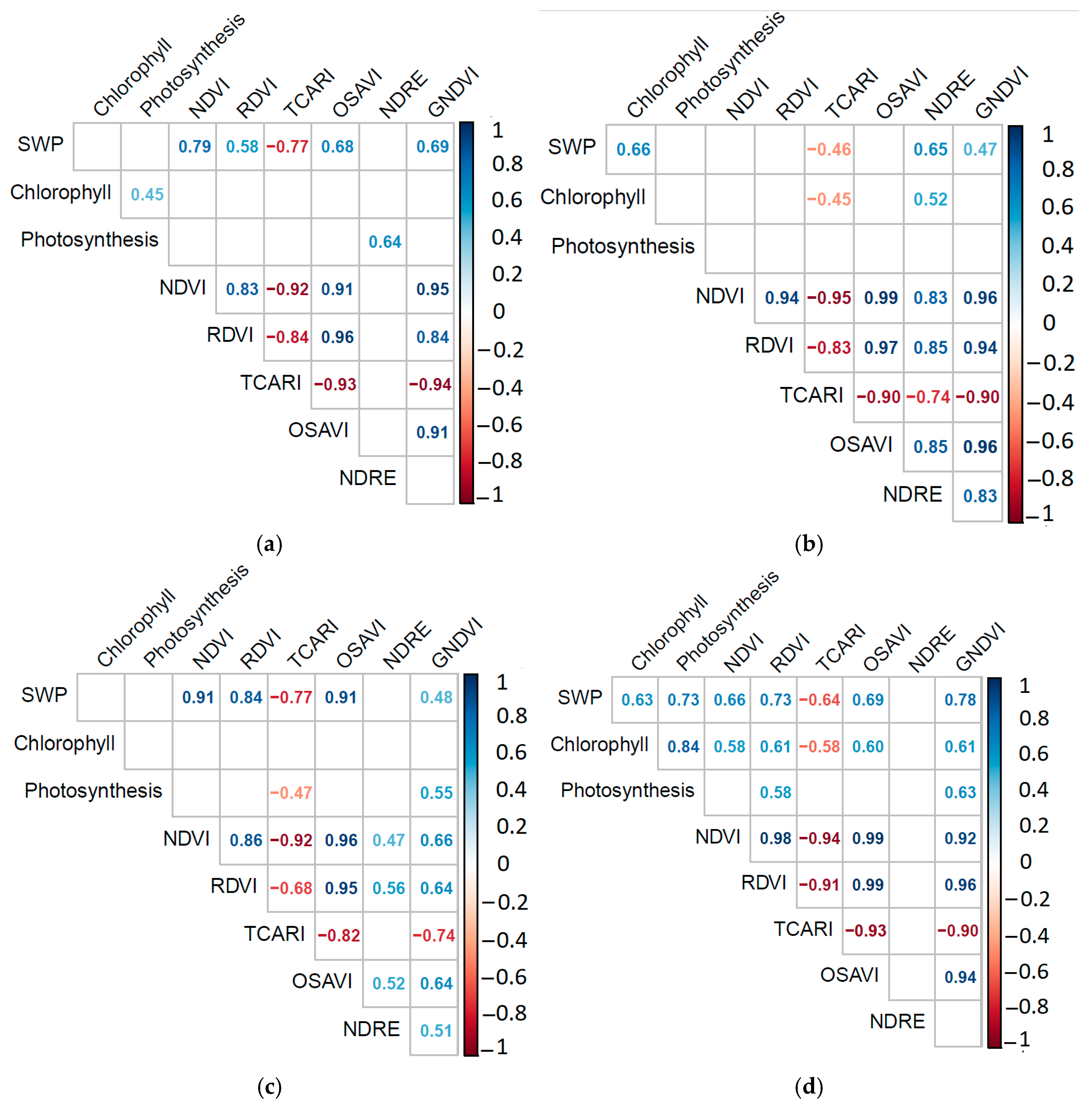
Figure 3 shows the Spearman correlation matrices illustrating the relationships between the SWP, chlorophyll, and photosynthesis and the spectral bands.

Chlorophyll showed moderate correlations (r > 0.5) in 2022 at both 09:00 and 12:00, associated with the green band in the first case and with both the green and red bands in the second. In contrast, photosynthesis did not exhibit significant correlations with any spectral band in any of the scenarios. The strongest relationships between the spectral bands and physiological variables were observed for the SWP, which showed significant correlations with the multispectral bands in all four scenarios, except at 09:00 in 2021. The highest r value was observed between the SWP and the red band at 12:00 in 2021 (r = −0.69) and the NIR band at 12:00 in 2022 (r = 0.67). The red band showed no correlation with the red edge band at any of the evaluated times of day. However, it was correlated with the green band at 09:00 in 2021 (Figure 3a), at 09:00 in 2022 (Figure 3b), and at 12:00 in 2022 (Figure 3d), as well as with the NIR band at 12:00 in 2022.

Figure 4 shows the Spearman correlation matrices illustrating the relationships between the SWP, chlorophyll, and photosynthesis and the VIs.

Photosynthesis and chlorophyll showed significant correlations with the VIs at 12:00 in 2022. The highest values were observed between chlorophyll and the GNDVI (r = 0.61), RDVI (r = 0.61), and OSAVI (r = 0.60). For photosynthesis, the strongest correlation was also with the GNDVI (r = 0.60). Photosynthesis showed a significant correlation with the NDRE at 9:00 in 2021 (r = 0.64) and GNDVI at 12:00 in 2021 (r = 0.55). Chlorophyll showed a moderate correlation with the NDRE at 09:00 in 2022 (r = 0.52).

The SWP exhibited statistically significant correlations with more VIs across the four evaluated scenarios than chlorophyll and photosynthesis. However, the SWP showed the smallest number of significant correlations at 9:00 in 2022; the only VI displaying a statistically significant correlation coefficient was the NDRE (r = 0.65).

Regarding the relationships between the VIs, strong correlations were observed among them across all evaluated scenarios. However, the NDRE did not show any correlation with the other indices at 12:00 in 2022 (Figure 4d).

Given that the SWP exhibited the most consistent relationships with the spectral bands and VIs, simple linear regression analyses were performed. The regression analyses were conducted using those spectral bands and VIs that exhibited a Spearman correlation coefficient with r > 0.5 in most of the evaluated scenarios (see Figure 3 and Figure 4). The strength of these relationships was assessed using the coefficient of determination (R²) (

Table 7. Coefficients of determination (R²) for the simple linear regression models where the stem water potential (SWP) was predicted using individual spectral bands (red) and vegetation indices (NDVI, RDVI, TCARI, OSAVI). Models were evaluated across different time points (9:00 and 12:00), years (2021 and 2022), and combinations of both. Sample sizes (n) are indicated for each comparison.

	2021		2022		21/22	21/22	2021/2022
	n = 25	n = 25	n = 20	n = 20	n = 45	n = 45	n = 90
	9:00	12:00	9:00	12:00	9:00	12:00	9:00/12:00
BAND
Red	0.21	0.40	0.30	0.30	0.61	0.44	0.50
VI
NDVI	0.61	0.78	0.19	0.46	0.54	0.65	0.60
RDVI	0.33	0.70	0.08	0.58	0.05	0.68	0.25
TCARI	0.50	0.57	0.19	0.54	0.48	0.65	0.53
OSAVI	0.42	0.77	0.14	0.53	0.21	0.69	0.43

).

The red band showed the highest coefficient of determination with the SWP, using data from 2021 and 2022 at 9:00 (R² = 0.61) and data from both years and both hours (R² = 0.50). Regarding the VIs, they showed better performance than individual bands. The strongest correlations (R² = 0.78) with the SWP were observed at 12:00 in 2021 with the NDVI. The NDVI, RDVI, TCARI, and OSAVI had better correlations with the SWP when using data at 12:00 from both years (2021 and 2022).

The NDVI showed the highest coefficient of determination (R²) when using combined data from both times of day (9:00 and 12:00) and both years, explaining up to 60% of the variability in the SWP.

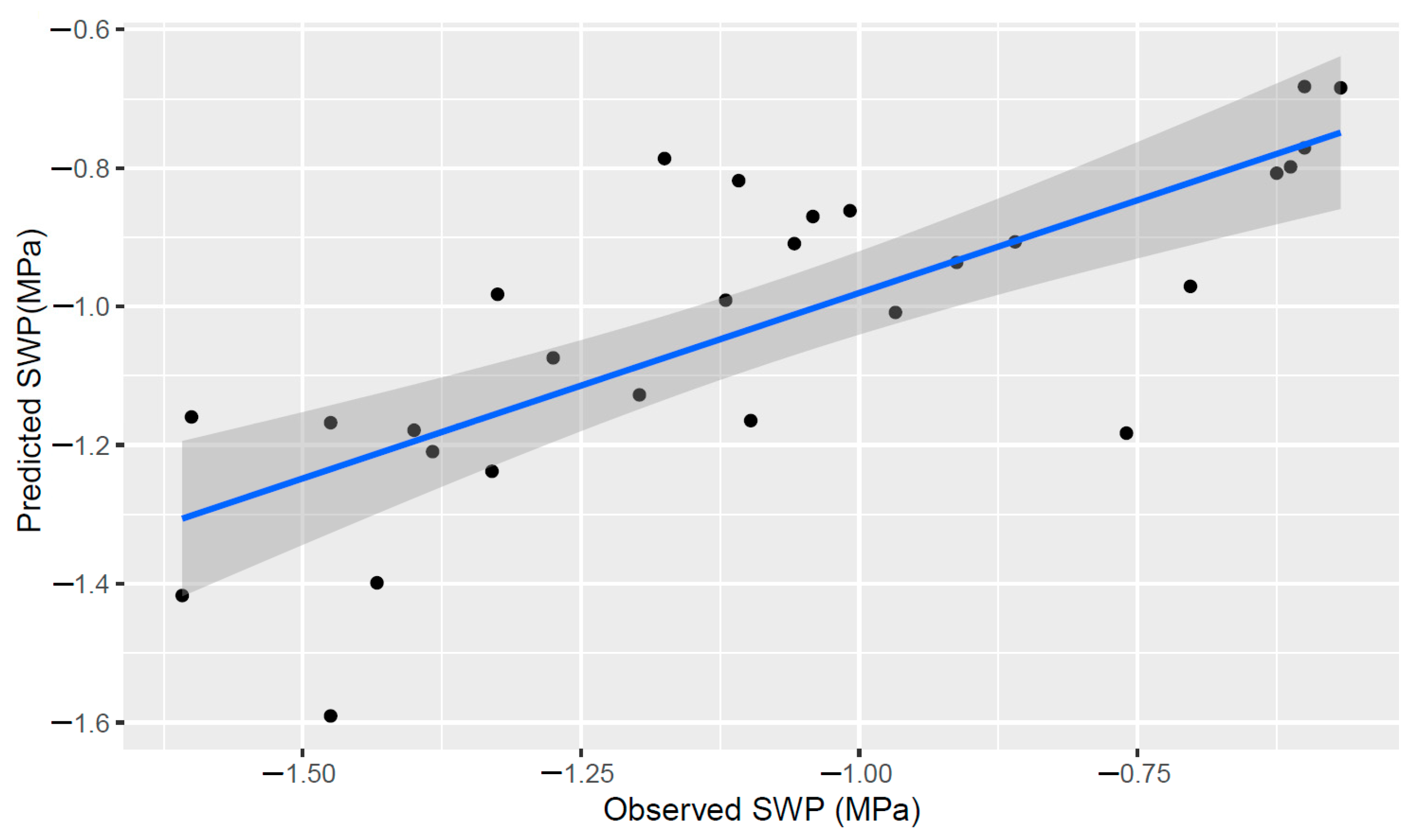
Given that the NDVI was the index that most consistently explained the variation in SWP across the evaluated scenarios, a 70/30 train–test split model was developed using the full dataset (both 2021 and 2022 seasons) to assess its overall predictive capacity.

Figure 5 illustrates the fitted regression model. The model achieved an R² of 0.58, RMSE of 0.22 MPa, MAE of 0.18 MPa, and MAPE of 18%. The equation of the model is

SWP = −4.3694 + 4.5288⋅NDVI

(3)

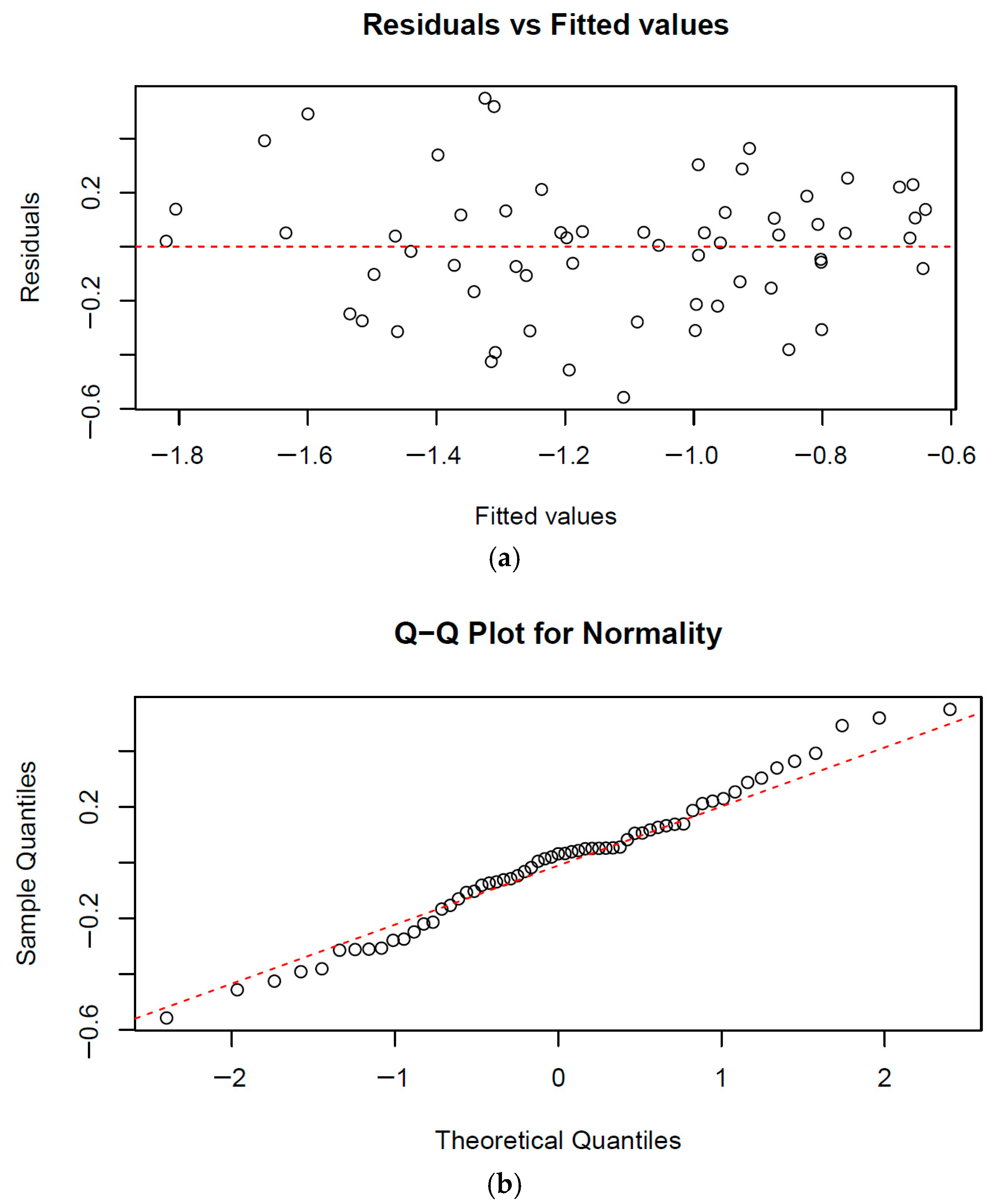
The residual analysis supported the model assumptions. The residual vs. fitted value plot (Figure 6a) shows a relatively random scatter around zero, indicating no strong evidence of heteroscedasticity. Additionally, the Q–Q plot (Figure 6b) demonstrates that the residuals are approximately normally distributed, with only minor deviations at the tails, suggesting that the model satisfies the normality assumption reasonably well.

3.5. Multiple Linear Regression Model of Spectral Bands with SWP

Additionally, a multiple linear regression model was developed using a 70/30 train–test data split, incorporating measurements from both 2021 and 2022 at 09:00 and 12:00. During model development, the green and red edge bands were found to have p-values greater than 0.05, indicating a lack of statistical significance.

To further support their exclusion, multicollinearity was assessed using the variance inflation factor (VIF). Both the green and red edge bands exhibited VIF values above 10, confirming the high degree of collinearity. Consequently, these bands were removed from the final model, as they did not contribute meaningfully to the prediction of the SWP.

The final model included only the red and NIR bands as predictor variables, both of which had acceptable VIF values (red: 1.15; NIR: 1.15), indicating low collinearity and stable contributions to the model.

The equation obtained was as follows:

SWP: −0.837 − 15.368⋅RED + 1.859⋅NIR

(4)

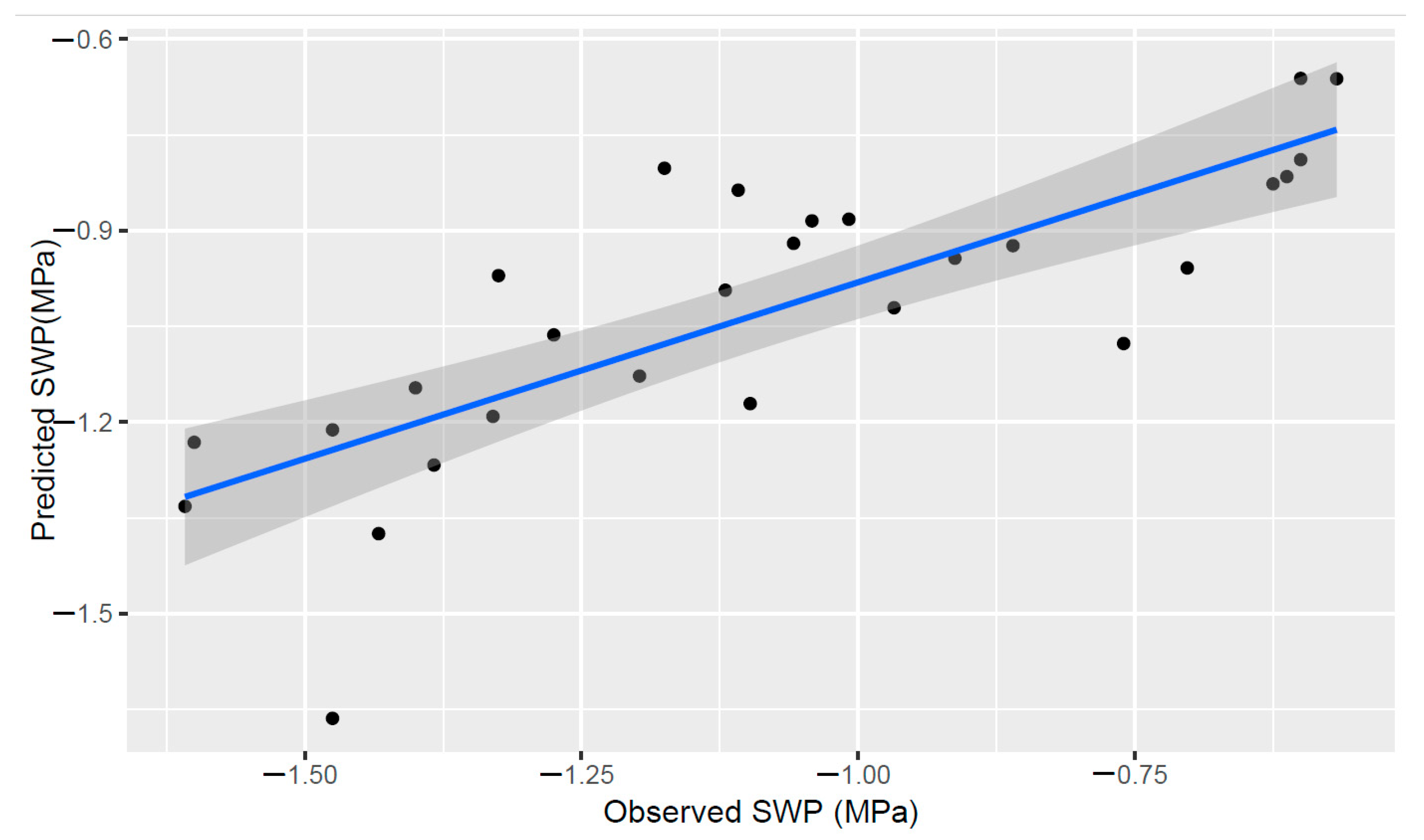
The performance of the multiple linear regression model was evaluated using the coefficient of determination R², which was 0.62; the RMSE, which was 0.20; the MAE, which was 0.18; and the MAPE, which was 17.6%. These indicated a moderate predictive capacity. Figure 7 shows the relationship between the predicted and observed stem water potential (SWP) values using the multiple regression model.

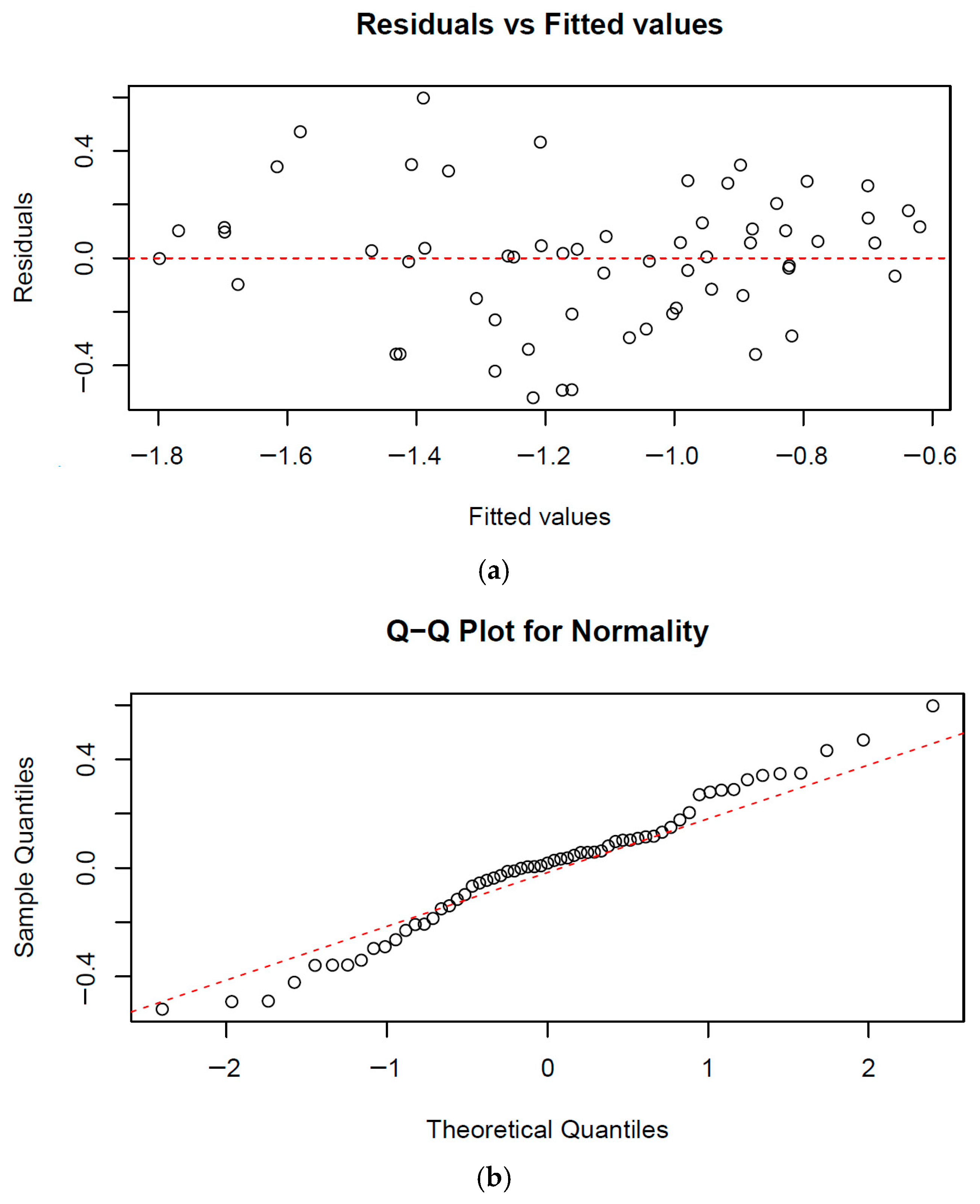
Figure 8 shows the error plots evaluated. Figure 8a shows the residuals vs. fitted values. The residuals appear randomly scattered around zero, indicating no clear pattern and supporting the assumption of homoscedasticity. Figure 8b shows that the data points closely follow the reference line, suggesting that the residuals are approximately normally distributed.

The Shapiro–Wilk test confirmed the normality of the residuals for the model, with W values close to 1 and non-significant p-values (W = 0.98237, p-value = 0.5252). These results indicate that the residuals follow a normal distribution, fulfilling a key assumption of linear regression and supporting the statistical validity of the models.

4. Discussion

The experiment provided a wide range of climatic and plant water status conditions. Specifically, 2022 was warmer and drier than 2021, with higher temperatures and lower relative humidity (Figure 2, Table 2). These climatic conditions likely contributed to the lower values in the vine physiological indicators. Specifically, the photosynthesis and chlorophyll content measured in 2022 were considerably lower than in 2021, both at 9:00 and at 12:00 (Table 3). This decline coincided with more negative SWP values, indicating that the 2022 growing season was characterised by more severe water stress. These results are consistent with the well-documented threshold for photosynthetic decline under water stress. Specifically, photosynthetic activity has been reported to decrease sharply at leaf water potentials (Ψf) below −1.0 MPa [38,39]. Our data support this pattern, as the observed reductions in photosynthesis under more negative SWP values align with the classic two-phase response: initial stomatal limitation under moderate stress, followed by non-stomatal impairment under severe water deficits [40,41].

The environmental conditions differed notably between 09:00 and 12:00, particularly in terms of the air temperature (Ta), relative humidity (RH), and vapor pressure deficit (VPD). As expected, the temperatures increased from morning to midday in both years, accompanied by a decrease in RH and an increase in VPD. These conditions reflect the typical intensification of the atmospheric water demand throughout the day, which directly affects the plant water status and gas exchange.

The lowest values of the SWP and photosynthesis were observed at 12:00, particularly in 2022. The high VPD values, driven by elevated temperatures, likely limited photosynthetic activity during midday. In contrast, the chlorophyll content did not show notable variation between different times of day; however, a reduction was observed in 2022, with lower mean values recorded compared to 2021.

The chlorophyll content appeared less sensitive to the irrigation treatments compared to photosynthesis and the SWP. These results suggest that the water status and chlorophyll content may respond independently to stress. Similar findings were reported in [42], where the authors observed that chlorophyll was not a reliable indicator of the grapevine water status. This aligns with broader evidence that extreme climatic conditions, such as those in 2022, can significantly alter physiological traits in plants [43].

The agronomic performance was also consistent with the observed physiological indicators of water stress. The berry weight (Table 4) decreased markedly across all treatments, particularly in T0 (rainfed).

In terms of vegetative growth (Table 4), the pruning weight was lower in deficit irrigation treatments, particularly in T0 and T50, and this effect was more pronounced in 2022. This trend reflects the reduced carbon assimilation capacity typically associated with water stress, as limited photosynthetic activity under such conditions constrains biomass accumulation [41,44].

Among the physiological parameters used to assess the plant water status, the SWP has traditionally been the standard tool in correlating the environmental conditions with the vine water status. The SWP provides a comprehensive measure that integrates soil, plant, and atmospheric conditions related to the water available to the plant [9,10]. In our study, the SWP varied notably across irrigation treatments and times of day and between years. In 2021, the values ranged from −0.6 MPa in well-irrigated treatments (T100, T50) to −1.1 MPa in the rainfed treatment (T0) at midday. In 2022, the overall SWP values were more negative, reaching −1.6 MPa in T0 at 12:00, indicating more severe water stress under higher evaporative demands. This is consistent with previous studies showing that the SWP becomes more negative under increasing vapor pressure deficits (VPDs) and reduced soil moisture availability [13,14]. Time-of-day effects are also well documented, with midday measurements typically reflecting the maximum stress levels due to the peak transpiration demand [15,16].

According to the literature, SWP values higher than −1.0 MPa are generally considered to reflect non-stressed or mildly stressed conditions in grapevines during midday. In contrast, values between −1.2 MPa and −1.4 MPa represent moderate stress, while values below −1.5 MPa are indicative of severe water stress, particularly in warm climates and during periods of high atmospheric demand [4].

Therefore, treatments T25, T0, and T25-S consistently experienced moderate to severe water stress, especially at midday, which correlates well with the reductions observed in photosynthesis and highlights the sensitivity of the SWP to both the irrigation strategy and environmental conditions. However, measuring the SWP is time-consuming and impractical for large-scale areas. In recent years, remote sensing technology using high-resolution images has been increasingly studied as a non-invasive method of estimating the vineyard water status. In our study, the strongest and most consistent relationships with the SWP were observed for the spectral bands and vegetation indices (VIs), rather than indices related to the chlorophyll content or photosynthetic activity (Figure 3 and Figure 4). These relationships demonstrate that spectral information can be effectively used to estimate the SWP, where linear regression models showed meaningful levels of accuracy (Table 7), particularly when combining data from multiple years and measurement times. The highest coefficients of determination (R²) were obtained at 12:00 for both years (2021 and 2022) and when data collected at both 09:00 and 12:00 across the two seasons (2021 and 2022) were pooled.

VIs tended to correlate more strongly with the SWP than individual spectral bands (Table 7). The NDVI, OSAVI, GNDVI, and TCARI presented the strongest relations at 12:00 with the SWP for both years (2021 and 2022) and when data were collected at both 09:00 and 12:00 across the two seasons (2021 and 2022). The NDVI-SWP relationship improved from R² = 0.54 (09:00) and R² = 0.67 (12:00) when analysed separately to R² = 0.60 when combining both times. This aligns with previous findings showing that VIs can integrate spectral information across bands, capturing complex physiological responses such as stomatal closure, pigment degradation, and reductions in mesophyll conductance [45,46,47,48,49]. In this context, the NDVI has been reported to be a good indicator of vegetative vigour, yields, and plant water status [50]. Ref. [22] reported the strongest correlations with the SWP, ranging between R² = 0.58 (GNDVI) and 0.68 (NDVI), as well [51], where the authors used a simple linear regression to predict water stress through VIs, finding R² > 0.7. Although relationships between the spectral bands and VIs and the SWP were observed at both measurement times, stronger correlations were consistently found at 12:00, suggesting that midday conditions may enhance the spectral sensitivity to the plant water status. Ref. [22] observed that indices such as the NDVI reflect long-term plant responses to water stress.

As a result, high determination coefficients were found for the linear regression between the VIs and SWP, with stronger correlations typically observed at 12:00. However, a robust model for the estimation of SWP must be independent of the specific measurement time or growing season. Integrating data from different times of day and from multiple years increases the robustness of the model by capturing a broader spectrum of physiological responses and environmental variability. In this context, the best-performing regression was obtained using the NDVI, based on a combined dataset covering both times of day and both years, achieving R² = 0.60. Therefore, this approach of combining datasets not only improves the statistical performance but also increases the potential for the practical application of spectral tools in vineyard water status monitoring, particularly under variable climate scenarios.

While VIs are widely used and have proven effective in many contexts, they are nonlinear combinations of spectral bands, which can introduce additional complexity in both their computation and interpretation.

If we focus specifically on the spectral bands, the red band alone showed notable predictive capacity in estimating the SWP (Table 7); the remaining spectral bands—green, red edge, and NIR—did not individually exhibit strong predictive power when used in isolation. However, their relevance lies in the significant correlations that they displayed with the SWP across different measurement times and environmental conditions, as shown in the Spearman correlation matrices (Figure 3a–d). These relationships justify their inclusion in the multiple linear regression model, as each band contributes complementary physiological information depending on the plant’s water status and the timing of measurement [52,53,54].

Multivariable and simple linear regression analyses are attractive because of their fast performance [55]. Ref. [19] have proven the possibility to monitor seasonal changes in SWP throughout the growing season in a vineyard using simple linear regression. In our study, the relationship between the NDVI and SWP, using data from both times of day and across the entire season, was significant, with R² = 0.60 (Table 7). This index includes the red and NIR bands, as noted before, which are both predictors of water stress. Similarly, Ref. [56] found a strong correlation between the NDVI and water treatments over two seasons. In contrast, indices such as the RDVI, TCARI, and OSAVI showed a better relationship with SWP measurements taken at 12:00 but not at 09:00. This temporal dependency may be attributed to the plant’s physiological response to solar radiation and water stress, which tends to be more pronounced at midday.

Regarding the multiple linear regression model, our results showed that the red and NIR bands could explain 62% of the variability. The green and red edge bands were not significant for SWP prediction. In general, the red and NIR spectral regions have been proposed as useful for the long-term monitoring of the vine water status [20,34,57]. Multiple linear regression was applied using only individual spectral bands, aiming to reduce the model complexity and avoid redundancy associated with Vis [58]. Simple and complex approaches have been used to model water stress indices with remote sensing data. Each presents advantages and disadvantages depending on the context of application.

In agriculture, artificial neural network (ANN) models are among the most widely used machine learning (ML) tools for crop management, water management, and soil management approaches [27]. Several studies have applied ANN models to estimate the vine water status using aerial imagery. Ref. [28] used multispectral images to calculate vegetation indices (VIs), achieving a correlation of R² = 0.53 between the simulated and measured SWP. Similarly, Ref. [28] employed ANN models using individual spectral bands as inputs, obtaining R² values between 0.56 and 0.87. Ref. [13] combined RGB imagery, multispectral bands, and the GCC index (representing canopy vigour) as inputs to ANN models, with R² = 0.98. However, these studies also highlight that the interannual variability of the crop, influenced by biotic and abiotic factors, affects the robustness and consistency of water status prediction models across different seasons. On the other hand, we can use simple models. These models are often easier to interpret and require fewer computational resources, while complex models (e.g., machine learning or deep learning) may capture nonlinear patterns more effectively but demand extensive training data and greater technical expertise.

Despite its simplicity, the multivariable modelbased on the red and NIR spectral bands development in this study demonstrated a moderate capacity to estimate the SWP under diverse field conditions. However, it has a tendency to overestimate the SWP values—especially in less stressed vines—and it assumes linearity and may not fully capture physiological responses under extreme conditions. Minor deviations in the residual distribution (Figure 8) were observed. Moreover, further validation is needed to assess its transferability to other cultivars, environments, or sensor types. However, it is important to highlight that the model was developed and validated using data collected over two climatically different seasons and at two different times of day.

The model’s main advantages lie in its interpretability, minimal computational demands, and reliance on spectral bands that are widely accessible in standard UAV-mounted cameras. From an operational perspective, this approach could facilitate the generation of SWP distribution maps, enabling the classification of the vine water status into actionable stress categories, as noted in [17]. Therefore, the predicted SWP values could be effectively used to delineate irrigation zones and support decision-making in deficit irrigation strategies.

However, further validation will be essential to confirm the consistency and robustness of this approach across different cultivars, growing conditions, and sensor platforms.

5. Conclusions

This study demonstrates the practical utility of UAV-based multispectral imagery and simple and multivariable regression models in estimating the stem water potential (SWP) in vineyards across different seasons and times of day. Despite the model’s development across a broad range of flight times, the results suggested that midday acquisitions yielded stronger relationships between the spectral data and plant water status. The proposed models are interpretable, require minimal data preprocessing, and can be readily integrated into operational viticulture practices to support irrigation scheduling or identify stress thresholds. While the current study focused on a low-complexity framework, its results lay the groundwork for future research aiming to extend these models across seasons and environments—potentially incorporating deep learning techniques to enhance the prediction accuracy and spatial resolution where resources and data availability allow.