Urban Expansion Scenario Prediction Model: Combining Multi-Source Big Data, a Graph Attention Network, a Vector Cellular Automata, and an Agent-Based Model

Abstract

The construction of transition rules is the core and difficulty faced by the cellular automata (CA) model. Dynamic mining of transition rules can more accurately simulate urban land use change. By introducing a graph attention network (GAT) to mine CA model transition rules, the temporal and spatial dynamics of the model are increased based on the construction of a real-time dynamic graph structure. At the same time, by adding an agent-based model (ABM) to the CA model, the simulation evolution of different human decision-making behaviors can be achieved. Based on this, an urban expansion scenario prediction (UESP) model has been proposed: (1) the UESP model employs a multi-head attention mechanism to dynamically capture high-order spatial dependencies, supporting the efficient processing of large-scale datasets with over 50,000 points of interest (POIs); (2) it incorporates the behaviors of agents such as residents, governments, and transportation systems to more realistically reflect human micro-level decision-making; and (3) by integrating macro-structural learning with micro-behavioral modeling, it effectively addresses the existing limitations in representing high-order spatial relationships and human decision-making processes in urban expansion simulations. Based on the policy context of the Outline of the Beijing–Tianjin–Hebei (BTH) Coordinated Development Plan, four development scenarios were designed to simulate construction land change by 2030. The results show that (1) the UESP model achieved an overall accuracy of 0.925, a Kappa coefficient of 0.878, and a FoM index of 0.048, outperforming traditional models, with the FoM being 3.5% higher; (2) through multi-scenario simulation prediction, it is found that under the scenario of ecological conservation and farmland protection, forest and grassland increase by 3142 km², and cultivated land increases by 896 km², with construction land showing a concentrated growth trend; and (3) the expansion of construction land will mainly occur at the expense of farmland, concentrated around Beijing, Tianjin, Tangshan, Shijiazhuang, and southern core cities in Hebei, forming a “core-driven, axis-extended, and cluster-expanded” spatial pattern.

1. Introduction

With the accelerating process of global urbanization, land use patterns have undergone profound change, posing dual challenges to both economic development and ecological conservation [1]. It is reported that global urban land expanded by 58% from 1992 to 2015, directly causing a loss of ecosystem service value of approximately USD 3.8 trillion, which severely threatens global ecological security [2]. Although urban expansion can stimulate regional economic growth, it often leads to negative effects such as population over-concentration, traffic congestion, and low land use efficiency if not accompanied by proper planning and resource management [3,4]. In response, international frameworks such as the Paris Agreement and the European Green Deal advocate compact cities and ecologically oriented urbanization models [5]. In China, urban agglomerations have become important platforms for promoting new-type urbanization [6,7], yet challenges such as internal development imbalance and the depletion of land reserves persist [8]. As one of China’s key economic hubs, the Beijing–Tianjin–Hebei (BTH) urban agglomeration benefits from regional economic integration but also faces severe issues, including air pollution, resource scarcity, and spatial inequality [9]. The Outline of the BTH Coordinated Development Plan explicitly proposes a green and low-carbon development path, emphasizing enhanced collaboration in transportation, industry, and ecological management within the urban agglomeration. Understanding the dynamic changes and development patterns of land use in the BTH region is of great significance for optimizing regional spatial structures, formulating targeted land policies, and achieving high-quality coordinated development.

In recent years, driven by advances in remote sensing (RS) and geographic information system (GIS) technologies, significant progress has been made in urban expansion modeling [10,11]. Research trends indicate that the dynamic process of rapid urbanization is not limited to land use change [12], but is intertwined with complex social, economic, and environmental issues [13,14]. Traditional modeling methods, including linear models, are easy to interpret and implement but have limitations in handling nonlinear relationships and spatial heterogeneity [15]. Cellular automaton (CA) models are widely used for simulating the dynamic evolution of spatial patterns and have become an essential tool in urban expansion studies. However, conventional CA models mostly rely on local neighborhood features and struggle to effectively capture spatial heterogeneity and complex temporal dynamics [16]. To overcome these limitations, machine learning (ML) and deep learning (DL) methods have been increasingly integrated into CA frameworks to improve the spatiotemporal accuracy of urban expansion simulations [17,18,19,20]. For example, Xun proposed a CA–random forest (RF) coupling model to simulate land use change by leveraging RS data and geographic information, significantly improving simulation accuracy [21]. Geng developed a spatiotemporal convolutional CA (ST-CA) model using 3D-CNN to accurately characterize the nonlinear spatiotemporal evolution associated with land use/cover change (LUCC) [22]. Xu further enhanced simulation accuracy in complex geographical environments by coupling CA with artificial neural networks (ANNs) [23]. Additionally, Qian et al. introduced an ANN-based CA transition rule combined with regional partitioning and spatiotemporal convolution, which considered subregional spatial heterogeneity and advanced land use change simulation methods [24]. Despite these improvements, most existing CA-ML/CA-DL coupling models still rely on fixed neighborhood structures and local spatial assumptions. They typically ignore the dynamic weight distribution among neighboring cells, which limits their ability to model complex high-order spatial dependencies and evolutionary mechanisms in urban expansion processes.

Graph neural networks (GNNs) have recently emerged as a breakthrough in spatial relationship modeling. Unlike traditional machine learning methods, GNNs incorporate adjacency matrices to comprehensively aggregate neighbor features and effectively capture long-range spatial dependencies [25,26]. Among these, the graph attention network (GAT) has demonstrated strong potential in modeling CA transition rules, owing to its ability to adaptively learn heterogeneous relationships between neighbors [27]. Furthermore, the development of the vector cellular automata (VCA) model allows point-based cells (e.g., POIs and pixel centers) to be efficiently involved in spatial modeling [28,29], further enhancing simulation accuracy and flexibility. Building upon this, Guan et al. proposed the HGAT-VCA model, which was the first to integrate high-order GAT with VCA, effectively learning complex high-order spatial dependencies and demonstrating improved simulation accuracy and neighbor configuration efficiency [30]. However, existing studies still primarily focus on spatial structure optimization and lack systematic consideration of micro-level agents and urban expansion simulations under multi-scenario and complex policy constraints. Therefore, developing a unified modeling framework that integrates high-order spatial modeling, micro-level behavioral decision-making, and multi-scenario forecasting has become an urgent research priority.

Moreover, macro–micro coupling modeling has become an essential trend in urban expansion studies [31]. Although traditional CA models perform well in simulating spatial evolution [32], they fail to capture micro-social behaviors and individual decision-making processes. To address this gap, recent studies have explored CA-ABM coupling frameworks, where ABM can simulate social behavior factors such as residents’ preferences and government planning from a micro-level perspective [33,34], thus improving the explanatory power of human activity influences [35]. Overall, multi-model coupling has become a key trend for enhancing both the simulation accuracy and mechanism interpretability of urban expansion [36,37].

To address these limitations, this study proposes a novel urban expansion scenario prediction (UESP) model that integrates GAT, VCA, and ABM into a unified framework. The UESP model systematically combines macro-level spatial structure modeling, high-order spatial interaction learning, and micro-level individual behavior simulation, enabling large-scale, multi-agent urban expansion simulations. Specifically, the model employs a high-order GAT with sparse adjacency matrix optimization to automatically learn CA transition rules through deep learning. Additionally, it incorporates ABM to simulate the influence of individual behavioral preferences on land conversion intentions, addressing existing limitations in spatial heterogeneity modeling, high-order dependency learning, and micro-level social behavior representation. To enhance the practical value of the UESP model, we designed four future urban expansion scenarios under the policy guidelines of the BTH Coordinated Development Plan, including ecological conservation, cultivated land protection, inertial development, and economic orientation. By predicting the land use patterns of the BTH region in 2030, this study aims to reveal spatial differences in urban expansion responses under policy interventions and support the formulation of optimized land use policies to facilitate sustainable regional development.

2. Study Area and Data

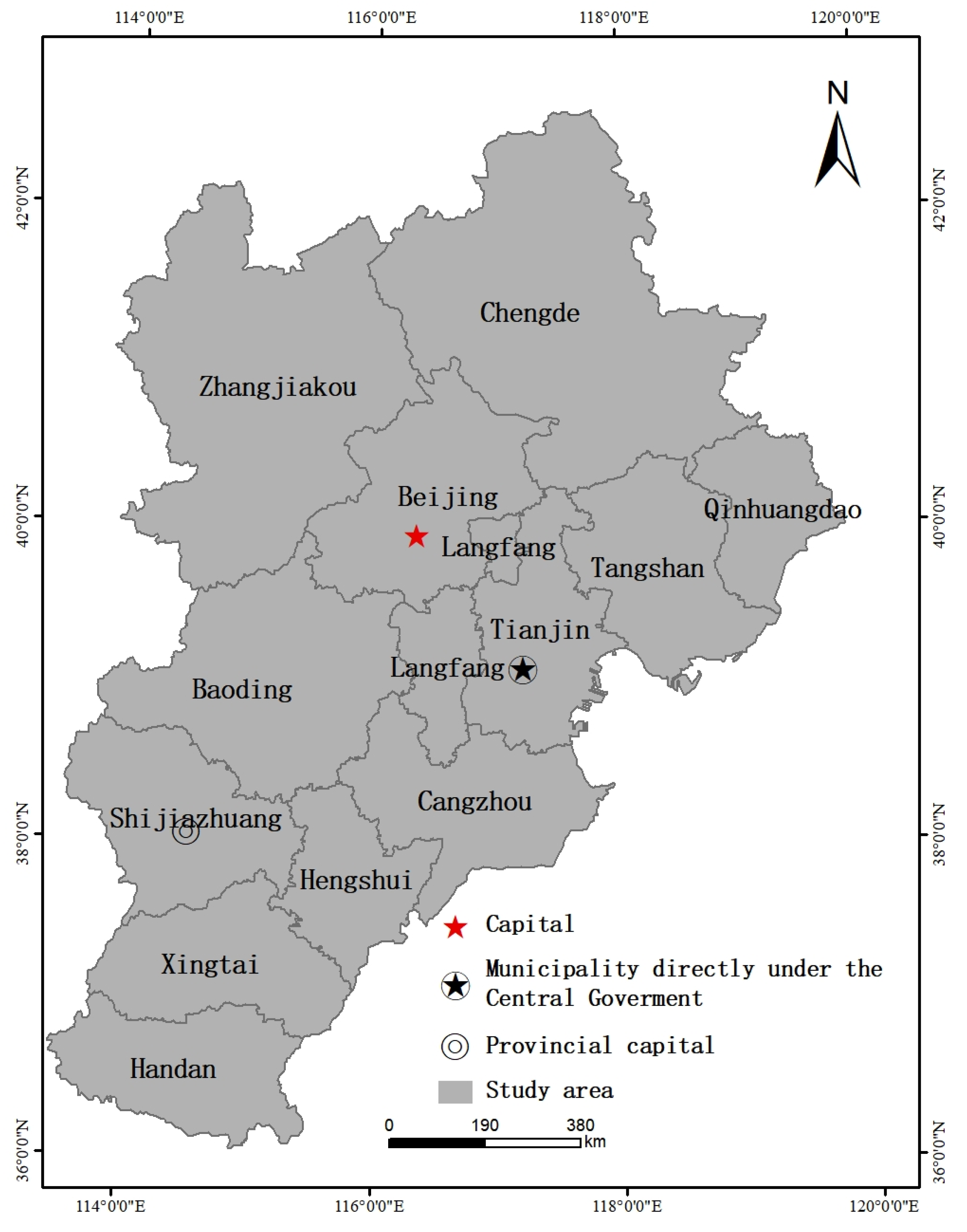
2.1. Study Area

The BTH region is located in northern China, between 36°03′N and 42°40′N and 113°27′E and 119°50′E. It comprises the two municipalities of Beijing and Tianjin and 11 prefecture-level cities in Hebei Province, including Baoding, Tangshan, Langfang, Shijiazhuang, Qinhuangdao, Zhangjiakou, Chengde, Cangzhou, Hengshui, Xingtai, and Handan. The BTH region is China’s capital economic circle (Figure 1). As the largest and most dynamic region in northern China, it plays an important role in China’s political and economic development [38]. As of the end of 2020, the total area of the BTH region is approximately 218,000 square kilometers, with a combined regional GDP of CNY 8639.3 billion, accounting for 8.5% of the national total [39].

The population in the BTH region has been growing rapidly. Driven by accelerated urbanization and economic development, resource consumption has surged, intensifying the conflicts among population growth, economic development, land demand, and ecological preservation. Extensive land use patterns are prevalent, and forest ecosystems have suffered severe degradation. The ecological and environmental pressures associated with urbanization, the spatial conflicts in resource utilization, and the shortcomings in regional infrastructure are expected to become increasingly severe [40]. In response to these challenges, the formulation of effective land use development strategies has become a priority to ensure long-term regional sustainability in the BTH region.

2.2. Data

This study employed multi-temporal land use maps as well as natural environment and socioeconomic driving factors. The land use data, provided by Wuhan University, covered three time periods: 2000, 2010, and 2020. The remote sensing data for 2000 and 2010 were primarily derived from Landsat 5 TM, supplemented by Landsat 7 ETM+ imagery. For 2020, Landsat 8 OLI data were predominantly used to ensure spectral consistency across the datasets. The data extracted multiple temporal features, including spectrum, phenology, and topography, and were generated through a combination of manual visual interpretation and random forest classification. The classification results exhibited high accuracy, with an overall accuracy of about 0.8 and a Kappa coefficient of 0.85 [41]. According to the land use classification standards published by the Chinese Academy of Sciences, the original land categories were reclassified into four types according to the following land use codes: cultivated land, forest and grassland, water area, and construction land. Given the low proportion of unused land and the fact that the amount of grassland within the study area is small and mostly distributed in forest land, they were uniformly classified under the category of “forest and grassland”. All land use data had a spatial resolution of 30 m. To support simulation modeling, the original grid-based land use map was divided into 2000 m fishing grids, from which the land use type at each grid center was extracted for further analysis.

Urban land use is typically influenced by natural conditions, socioeconomic activities, and policy interventions [42]. A systematic review of the relevant literature is summarized in

Table 1. Frequency statistics of commonly used driving factors in land use change simulation studies.

References	DEM	Slope	Primary Roads	Highway	Social Service Facilities	Education	GDP	Population
Al-Kheder et al., 2008 [42]	1 √	√	√					√
Guan et al., 2023 [30]	√	√		√	√	√
Guan et al., 2024 [48]	√	√	√	√	√
He et al., 2006 [43]	√	√		√
Lau and Kam, 2005 [44]			√		√			√
Liang et al., 2020 [21]	√	√	√	√	√		√	√
Liu et al., 2020 [31]			√		√	√
Shen et al., 2008 [45]								√
Shi et al., 2023 [46]	√	√	√		√		√	√
Wu et al., 2022 [47]	√	√	√			√	√	√

¹ √ indicates the factors used by the authors to simulate land use change.

, which demonstrates the commonly selected driving factors and their usage frequency [21,30,31,42,43,44,45,46,47,48].

Based on data availability and accessibility, this study systematically considers socioeconomic and natural driving factors. Accordingly, a comprehensive driving dataset consisting of 11 variables was constructed, covering natural environmental factors, socioeconomic factors, and agent-based model related factors. Data sources and classification details are presented in

Table 2. Data used in this study.

		Data	Data Sources
Land use data		2000 Land use data	Landsat 5 TM, Landsat 7 ETM+
		2010 Land use data	Landsat 5 TM, Landsat 7 ETM+
		2020 Land use data	Landsat 8 OLI
Natural environment factors		DEM	Geospatial data cloud
		Slope	Geospatial data cloud
Socioeconomic factors		School features	OSM
		Mall features	OSM
		Bank features	OSM
		Hotel features	OSM
		Hospital features	OSM
		House features	OSM
		Restaurant features	OSM
		Main road features	OSM
		Highway features	OSM
ABM	Resident agents	Population	NBSC
		GDP	NBSC
	Traffic agents	Main road features	OSM
		Highway features	OSM

. The elevation data and slope data in this study are calculated based on the original DEM data. Nine socioeconomic factors include the Euclidean distance to schools, hotels, banks, restaurants, malls, hospitals, houses, main roads, and highways, which are calculated as the Euclidean distance between each pixel and its closest spatial entity of the respective type. To further reflect the impact of individual behavior on land use change, we introduce the ABM module into the CA model to simulate the behavior of resident agents and traffic agents. Resident agent-related factors mainly include GDP, population density, and commercial service facilities, while traffic agents consider factors such as road density and traffic accessibility. To eliminate the influence of differing dimensions, Min–Max normalization is applied to scale all patch characteristic values to a range between 0 and 1. All spatial variables are visualized in Figure 2. Finally, to improve the computational efficiency of large amounts of data, all data were resampled to a spatial resolution of 2000 m for land use simulation.

3. Methodology

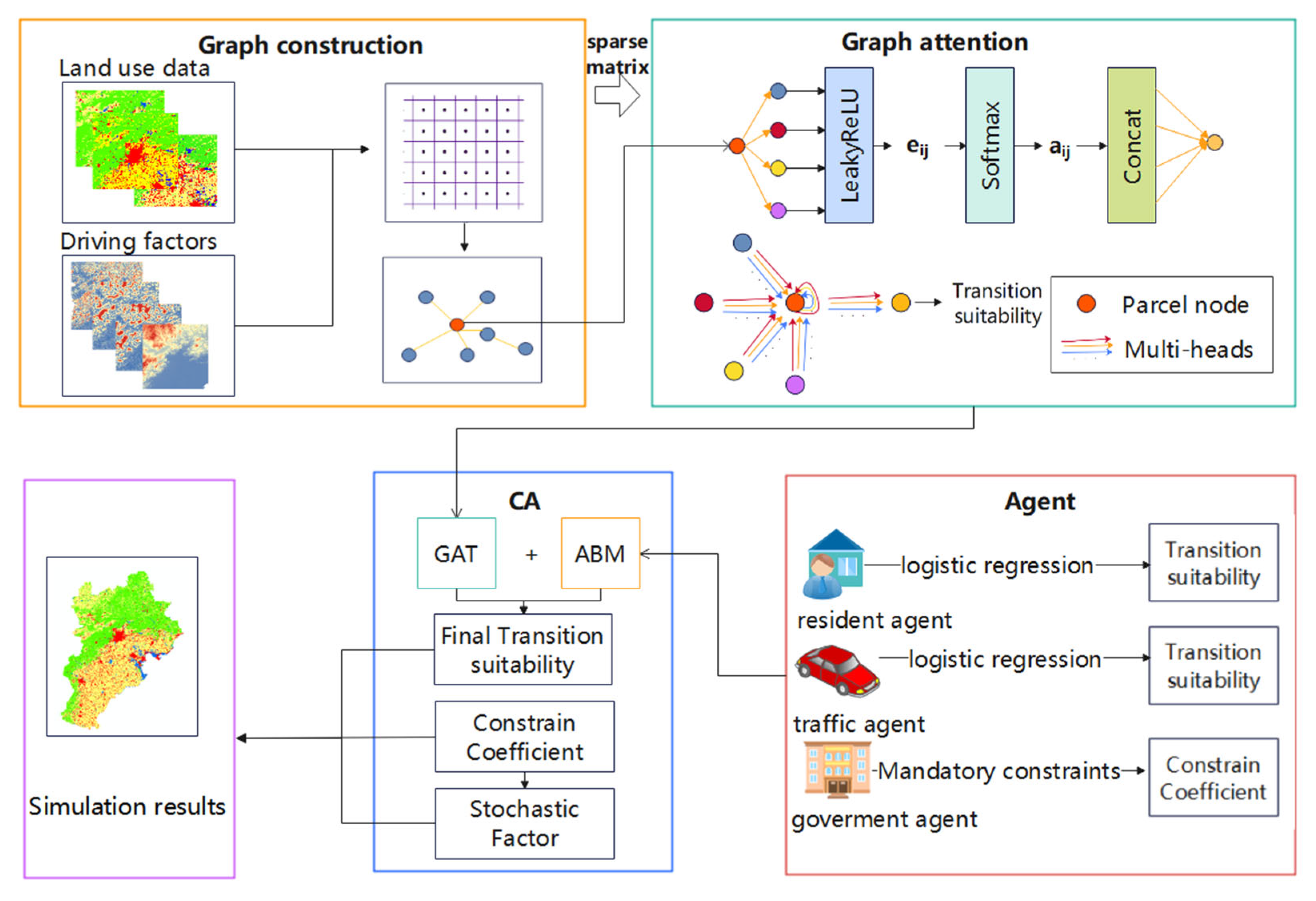
3.1. Overview

This paper proposes a UESP model framework (Figure 3), which mines the neighborhood transition rules of vector cellular automata through a graph attention network and integrates an agent-based model to simulate micro-behavioral decisions. The framework consists of three parts: (1) Graph structure construction and feature fusion based on land use data: the graph structure is generated based on multi-source remote sensing and geospatial datasets, with nodes representing cellular attributes and edges defining spatial adjacency relationships. (2) GAT mines CA neighborhood rules: the multi-head attention mechanism is employed to quantify the neighborhood interaction intensity and generate land use transition probability. (3) Coupling the graph attention network and the ABM-CA model: micro-behaviors, such as residents’ preferences and policy constraints, are embedded in cellular evolution rules through parameter mapping to achieve integrated simulation.

In this study, we conducted experiments at spatial resolutions of 500 m, 1000 m, 2000 m, and 5000 m. After comprehensively evaluating both simulation accuracy and computational efficiency, a resolution of 2000 m was ultimately selected for the final experimental analysis. The study area is divided into 2000 m grids. The centroid of each grid was used to extract both the corresponding land use type and driving factors, and these centroids served as nodes in the graph structure. This spatial scale enables the effective representation of the urban agglomeration patterns while significantly reducing computational costs, thereby ensuring efficient training and simulation performance of the graph neural network on large-scale datasets. Spatial adjacency relationships were used to define the edges, and nodes within a radius of 2828.5 m were connected by shared edges. The constructed node and feature information was then input into a graph attention network, which employs an attention mechanism to dynamically learn the importance weights between connected nodes, quantify neighborhood influences, fuse features, and generate land use conversion suitability probabilities.

Model parameters are optimized via a backpropagation-based loss function, enabling GAT to extract VCA neighborhood transition rules through deep learning. Subsequently, multi-source influencing factors—such as resident preferences, traffic convenience, and government constraints—are linearly integrated to incorporate human decision-making into the conversion rules. To efficiently handle large-scale datasets involving more than 50,000 vector grid cells, the model employs sparse matrix operations and parallelized high-order adjacency matrix calculations, effectively overcoming computational bottlenecks and ensuring efficient training and prediction.

3.2. GAT-VCA-ABM

3.2.1. GAT

(1)

Graph structure construction

Recently, graph neural networks (GNNs) have been introduced for modeling interactions, owing to their capacity to capture rich relational information between entities [49]. In order to enable nodes to selectively pay attention to neighboring nodes with high relevance, several special GNNs have been introduced, among which GAT is particularly popular and has been widely used in interaction modeling in many fields such as traffic prediction, social recommendation, behavior recognition, etc. [50,51].

First, a graph structure is constructed based on the land use data, which can be formulated as G(V, E, X, A). Here, the adjacency matrix $A\in {ℝ}^{\mathrm{N}\times \mathrm{N}}$ of the graph is used to represent the connectivity between nodes i and j in the graph, V is a set of nodes sampled from N patches, and E is the edge defined by the adjacency relationship of the nodes. The feature matrix X represents the M attributes of the corresponding patch, including land use types and driving factors. For vertex i, its relationship with the adjacent vertex j is defined as shown by Equation (1) [27].

$$A_{ij}=\left\{\begin{array}{c}1,j\in VN\left(i\right)\\ 0,otherwise\end{array}\right.$$

(1)

Here, VN(i) denotes the neighbor set of node i, determined by the spatial adjacency of patches. If patch i shares a common boundary or vertex with patch j, the relationship $A_{ij}$ is 1; otherwise, it is 0.

The k-order adjacency matrix used in this study is defined through iterative neighborhood expansion based on the original adjacency matrix. In each iteration, the neighbors of the current neighbors are identified, and all selected nodes collectively form the high-order adjacency structure. This process continues until the kth iteration is reached. Mathematically, the k-order adjacency matrix, denoted as $A^k$, is obtained by raising the original adjacency matrix A to the power of k − 1. The final high-order adjacency matrix ${\tilde{A}}^k$ is computed as the sum of adjacency matrices from the first to the nth order, illustrated by Equation (2):

$${\tilde{A}}^k={{\displaystyle \sum }}_{k=1}^k{A}^k$$

(2)

(2)

Graph Attention Operation

After the graph structure is constructed, the attention mechanism is employed to learn the attention coefficient of the connection point. The adaptability of the central node is determined by both the state characteristics of the central node and those of its neighbors. Specifically, if a neighboring patch has a stronger connection with the central patch i, then it exerts a greater impact on patch i and is assigned a higher aggregation weight. Graph attention computes the attention coefficient, which is then utilized to aggregate information from neighboring patches. The attention coefficient $e_{ij}$ between the central patch i and the adjacent patch j is shown in Equation (3):

$$e_{ij}=LeakyRelu\left({\overrightarrow{q}}^T\left(W{\overrightarrow{h_i}}^{\left(l\right)}\left|\right|W{\overrightarrow{h_j}}^{\left(l\right)}\right)\right), j\in N_i$$

(3)

Here, ${\overrightarrow{h_i}}^{\left(l\right)}\in {ℝ}^{d\times 1},\mathrm{i}=1,2,\dots ,\mathrm{n}$, represents the input feature of the center patch i in the lth layer, ${\overrightarrow{h_j}}^{\left(l\right)}\in {ℝ}^{d\times 1},\mathrm{i}=1,2,\dots ,\mathrm{n}$, represents the input feature of the adjacent patch j in the same layer, and d is the feature dimension. The feature vector ${\overrightarrow{h_i}}^{\left(l\right)}$ and the neighborhood feature vector ${\overrightarrow{h_j}}^{\left(l\right)}$ are, respectively, transformed linearly to obtain $W{\overrightarrow{h_i}}^{\left(l\right)}, W{\overrightarrow{h_j}}^{\left(l\right)}$, which highlight the differences between nodes and enhances the model’s feature representation capability. The symbol “$\left|\right|$” denotes feature concatenation, which merges two vectors together to form a ($2d^{\prime }$, 1) dimensional vector, and ${\overrightarrow{q}}^{T\in {ℝ}^{2F‘}}$ is a learnable vector to calculate attention. Finally, the activation function “$LeakyReLU$” is used to generalize the fitting ability of the model, and the attention coefficients of patches i and j are obtained [48].

When a node is connected to multiple neighboring nodes, the attention coefficients need to be normalized for fair comparison across neighbors. To prevent the model from overemphasizing a single neighbor node and neglecting others due to an excessively large attention coefficient, the normalization function $“softmax$” is applied to normalize the attention scores among adjacent nodes. The normalized attention coefficient $a_{ij }$ is then calculated through Equation (4):

$$a_{ij}=\sigma softmax\left(e_{ij}\right)={\displaystyle \frac{\mathit{exp}\left(e_{ij}\right)}{{{\displaystyle \sum }}_{k\in V{N}_i}\mathit{exp}\left(e_{ik}\right)}}$$

(4)

Then, to update the feature vector value of the central node, a normalized attention coefficient $a_{ij}$ is assigned to each neighbor node. The result after concatenation is output as Equation (5), where ${\overrightarrow{h_i}}^{\left(l+1\right)}\in {ℝ}^{d\prime }$,$\sigma$ denotes the activation function of $“sigmod”$, which is the final output feature of each node:

$${\overrightarrow{h_i}}^{\left(l+1\right)}=\sigma \left({\displaystyle \sum }_{j\in V{N}_i}{a}_{ij}W{\overrightarrow{h_j}}^{\left(l\right)}\right)$$

(5)

A single graph attention operation may suffer from limited expressiveness and may fail to capture key interactions with important neighboring nodes. To improve the robustness of the attention mechanism and to better capture the diversity of spatial interactions, a multi-head attention layer is introduced. This method performs multiple independent attention computations in parallel, allowing for a more comprehensive investigation of spatial dependencies among land patches. Accordingly, Equations (3)–(5) are reformulated as Equations (6)–(9).

$$e_{ij}^p=LeakyRelu\left({({\overrightarrow{q}}^p)}^T\left(W^p\overrightarrow{h_i}\left|\right|W^p\overrightarrow{h_j}\right)\right), j\in N_i$$

(6)

$$a_{ij}^p=softmax\left(e_{ij}^p\right)={\displaystyle \frac{\mathit{exp}\left(e_{ij}^p\right)}{{{\displaystyle \sum }}_{k\in N_i}\mathit{exp}\left(e_{ik}^p\right)}}$$

(7)

$${\overrightarrow{h_i}}^{\prime }={\mid \mid }_{p=1}^p\sigma \left({\displaystyle \sum }_{j\in V{N}_{\left(i\right)}}{a}_{ij}^p{W}^p\overrightarrow{h_j}\right)$$

(8)

Here, ${\left|\right|}_{p=1}^p$ denotes the concatenation of features from multiple attention heads, and p represents the number of these heads. In addition, the strength of heterogeneous interactions is effectively quantified through the selective aggregation process. Finally, a fully connected output layer is applied to compute the adaptability of land patch i to each land use type.

Specifically, ${a_{ij}}^{\left(l+1\right)}$ is the attention weights at the (l + 1)th layer, and $W^{out}$ represents the trainable weight matrix in the output layer, and $z_i\in {ℝ}^s$ is the output vector for land patch i, with a dimensionality corresponding to the number of land use class s patches. The final land use transition adaptability coefficient of cell i to land use type s is computed as shown in Equation (9), and the conversion probability of cell i to each land use type is obtained as defined in Equation (10).

$$z_i=ELU\left({\displaystyle \sum }_{j\in V{N}_{\left(i\right)}}{a_{ij}}^{\left(l+1\right)}{W}^{out}{\overrightarrow{h_j}}^{\left(l+1\right)}\right)$$

(9)

$$P_i^s={\displaystyle \frac{\mathit{exp}\left(z_{i,s}\right)}{{{\displaystyle \sum }}_{c^{\prime }=1}^C\mathit{exp}\left(z_{i,s^{\prime }}\right)}}$$

(10)

3.2.2. ABM

The transformation rules in the VCA model exhibit certain limitations, as they fail to incorporate human-related factors involved in the land use change process, including the influence of governments, developers, and residents. In contrast, the agent-based model can explicitly represent the behavioral rules of individual agents, thereby compensating for the limitations of traditional CA models in simulating micro-level decision-making processes. ABM consists of multiple interacting agents, each with dynamic behaviors and heterogeneous characteristics [52]. Within the model, agents interact with one another and with their surrounding environment, continuously adjusting their behaviors and decision-making strategies through mutual influence and learning. The dynamic evolution of land use emerges from the interactions between micro-scale spatial individuals as well as between individuals and their environment [53]. In this study, the relationship of ABM can be expressed as Equation (11):

$$U_i~\left(P_{resident}, P_{traffic}, P_{government}\right)$$

(11)

Here, $U_i$ represents the comprehensive impact of three different agents on land use change.

By introducing three different agents to influence the surrounding environment’s effect on the cells in the conversion rule and the restriction coefficient, human factors are more effectively integrated into the land use transformation process. The selection behavior of resident agents is closely related to the surrounding environment. Generally, people prefer to reside in areas with well-developed public facilities, a favorable environment, and moderate population density. After comprehensively considering various factors, the influencing factors of resident agents in this study include GDP, population density, and spatial distance to major facilities such as hospitals, schools, shopping malls, supermarkets, parks, hotels, restaurants, etc. The shorter the distance, the higher the accessibility of the facilities and the better the convenience of life. The values of these human-related factors were extracted at the centroid of each grid cell using ArcGIS 10.4 software and standardized to eliminate the impact of the dimension. This relationship can be expressed as follows:

$$P_{resident }= {\beta }_{GDP}{X}_{GDP}+{\beta }_{population}{X}_{population}+{\beta }_{houses}{X}_{houses}+{\beta }_{parks}{X}_{parks}+{\gamma }_1$$

(12)

Here, ${\beta }_{GDP}$, ${\beta }_{population}$, ${\beta }_{houses}$, and ${\beta }_{parks}$ represent the weights of GDP, population, residential convenience, supermarket accessibility, and park convenience, respectively; ${\beta }_{GDP}+{\beta }_{population}+{\beta }_{houses}+{\beta }_{parks}=$ 1, $X_{GDP}$, $X_{population}$, $X_{houses}$, and $X_{parks}$ represent the impact of regional GDP, population, residential convenience, and park convenience on land use change, respectively; and ${\gamma }_1$ is random interference.

The introduction of traffic agents represents the driving role of traffic conditions in land use decisions, and key factors considered include road network density and distance to major roads and highways, as formulated in Equation (13). High transportation connectivity can enhance the development potential of a region, exerting a particularly significant influence on the expansion of construction land.

$$P_{traffic }={\beta }_{roadDenisty}{X}_{roadDenisty}+{\beta }_{highway}{X}_{highway}+{\beta }_{mainRoad}{X}_{mainRoad}+{\gamma }_2$$

(13)

where ${\beta }_{roadDenisty}$, ${\beta }_{highway}$, and ${\beta }_{mainRoad}$ represent the weights of road density, highway convenience, and main road convenience, respectively; ${\beta }_{roadDenisty}+{\beta }_{highway}+{\beta }_{mainRoad}=$ 1, $X_{roadDenisty}$, $X_{highway}$, and $X_{mainRoad}$ represent the impact values of road density, highway convenience, and main road convenience on land use change, respectively; and ${\gamma }_2$ is random interference.

The introduction of a government agent reflects the top-down regulatory power of the government authorities, which is particularly prominent in the context of China. According to the Ecological Conservation Redline Delineation Guidelines, each province is required to define development-permitted and development-restricted zones. In this study, areas within the ecological redline boundary in the BTH region are designated as non-developable zones, while areas outside the redline are considered eligible for development. Additionally, during the 10- to 20-year planning period, portions of construction land in Tangshan, Hebei Province, were converted into reservoirs under government planning. Consequently, the government agent enforces a mandatory transformation of these areas into water area. $P_{government}$ represents binary data, indicating the mandatory constraints of the policy, where $P_{government}=0$ indicates that development is prohibited and $P_{government}=1$ indicates that development is allowed.

3.2.3. UESP Model Construction

(1)

CA

Cellular automata are top-down, dual-discrete micro-dynamic models that operate both in time and space. The core principle of CA is to reveal the overall evolution of complex systems through local interactions of simple rules [32,54]. Cells are scattered in a regular grid, take finite discrete states, follow the same transformation rules, and transform according to these determined local rules. It is the simple interactions among a large number of cells that constitute the evolution of the cellular automaton system.

In a conventional cellular automata model, space is discretized into a set of cells, each representing a geographic entity. Each cell possesses a finite number of states and evolves over a discrete space according to transition rules defined by its current state and the states of neighboring cells. A standard CA model typically consists of four essential components: cells, cell states, a cell neighborhood, and transition rules.

(2)

VCA

Building upon traditional CA, the vector-based cellular automata (VCA) model adopts a vector data structure, which is the fundamental distinction from conventional CA. VCA represent geographic entities in the study area using Euclidean geometric constructs such as points, lines, polygons, and polygonal complexes, thereby enabling a more accurate simulation of the irregularity of land parcels and improving the spatial resolution of the model [28,55]. In typical CA models, the transition rules of a cell’s state are determined by five key components: the present state of the cell, the suitability for transition, the states of neighboring cells, constraint factors, and stochastic disturbance. In this study, the current and neighboring cell states are structured as a graph and input into the GAT. Through deep learning, GAT effectively captures neighborhood dependencies and generates the land conversion suitability $P_i^{s,t}$. The specific transition rule in the VCA model is defined by Equation (14) [56].

$$O{P}_i^{s,t+1}=a_1{P}_i^{s,t}+a_2{R}_i^t+\gamma$$

(14)

Here, p is the adaptability of land conversion, which is derived from the current cell state and its neighbor relationship. $P_i^{s,t}$ represents the adaptability of cell $i$ to the transfer of land use type $s$, which is generated by the output layer of GAT through sparse matrix operations. $C_i^t$ represents the restriction coefficient of cell i at time t. If $C=1$, the cell can develop iteratively; otherwise, if $C=0$, it cannot develop. $R_i^t$ is a random factor, which represents the unknown external influences affecting patch i at time t. $R_i^t=1+{\left(-\mathit{ln}\gamma \right)}^{\alpha }$, $\gamma$ are disturbance factors with a value range of 0 to 1. $\alpha$ is used to control the interference intensity of the random disturbance term, which is a parameter from 1 to 10. $a_1$,$a_2$ represent the weights of the corresponding factors. In this study, for the convenience of calculation, let $a_1=a_2=1$. After computing the transition probability $O{P}_i^{s,t+1}$ of cell i at time t, the land use type with the highest probability is selected and then compared to the threshold. If the probability is higher than the threshold, the cell is converted to the corresponding land use type; otherwise, the cell state remains unchanged. The threshold is determined during the simulation process by the historical land use data based on the total changed area from time t to time t + 1.

In the process of land use change, land use units are influenced not only by their own land use types and those of their neighboring units but also by various socioeconomic and policy-related factors. Incorporating these diverse and interacting influences makes the land use evolution process inherently more complex. To better capture this complexity, this study further integrates an agent-based modeling (ABM) framework into the previously established GAT-CA transition function (Equation (13)) to simulate the decision-making behaviors of micro-level entities in land use transformation. Specifically, in modeling resident agents and transportation agents, this study employs a multinomial logistic regression model based on historical land use change data to capture the asymmetric relationships between multiple features and the transformation tendencies toward different land use types. This approach generates a behavior-driven probability distribution $U_i$ that reflects the willingness of each land parcel to convert into various land use categories. Finally, this behavior probability distribution is integrated with the macro-scale suitability probability $P_i^{s,t}$ generated by the graph attention network, forming a hybrid macro–micro land use simulation rule that more realistically reflects land transition dynamics.

In summary, at time t, the land transition probability of cell i toward land use type s is jointly determined by its transfer adaptability $P_i^{s,t}$, the random factor $R_i^t$, and the influence probability $U_i$ of the driving factors in ABM, which can be written as follows:

$$O{P}_i^{s,t+1}~f\left(P_i^{s,t},C_i^t,R_i^t,U_i\right)$$

(15)

3.3. Accuracy Assessment

This study adopted a point-by-point comparison method and used five quantitative indicators to evaluate the performance of the model [57,58]: figure of merit (FoM), producer accuracy (PA), user accuracy (UA), overall accuracy (OA), and Cohen’s Kappa coefficient (Kappa). The first three mainly reflect the accuracy of the changes in the simulation. PA and UA represent the omission and commission rates of the predicted results for each land use type, respectively. These are calculated based on the cells that have changed, while cells that remain unchanged during the simulation process are ignored. This method enables a more comprehensive assessment of the model’s performance, with evaluation values ranging from [0, 100%]. OA measures the agreement between the simulated and actual land use patterns in the target year, within a range of 0% to 100%. For Kappa, the range is [0, 1]. For these indicators, values greater than 80% or 0.8 indicate better model performance.

$$PA={\displaystyle \frac{B}{A+B+C}}$$

(16)

$$UA={\displaystyle \frac{B}{B+C+D}}$$

(17)

$$Fom={\displaystyle \frac{B}{A+B+C+D}}$$

(18)

Here, A represents the area of the patch where the observed change is predicted to be a persistent change (i.e., no change), B represents the area of the patch where the observed change is simulated as a change, C represents the area of the patch where the observed change is predicted to be an incorrect gain, and D represents the area of the patch where the observed persistent change is predicted to be a change (actual change, predicted to be no change).

$$OA={\displaystyle \frac{{{\displaystyle \sum }}_{u=1}^{m}Coun{t}_{uu}}{ALL}}$$

(19)

$$Kappa={\displaystyle \frac{N{{\displaystyle \sum }}_{i=1}^C{x}_{ii}-{{\displaystyle \sum }}_{i=1}^C(x_{i+}\times x_{+i})}{N^2-{{\displaystyle \sum }}_{i=1}^C(x_{i+}\times x_{+i})}}$$

(20)

where N represents the total number of elements in the error matrix, C is the number of rows in the error matrix, x_ii denotes the element on the diagonal of the error matrix, that is, the element whose simulation results are the same as the real data, x_i+ is the sum of the elements in the ith row, and x_+i is the sum of the elements in the ith column.

4. Results

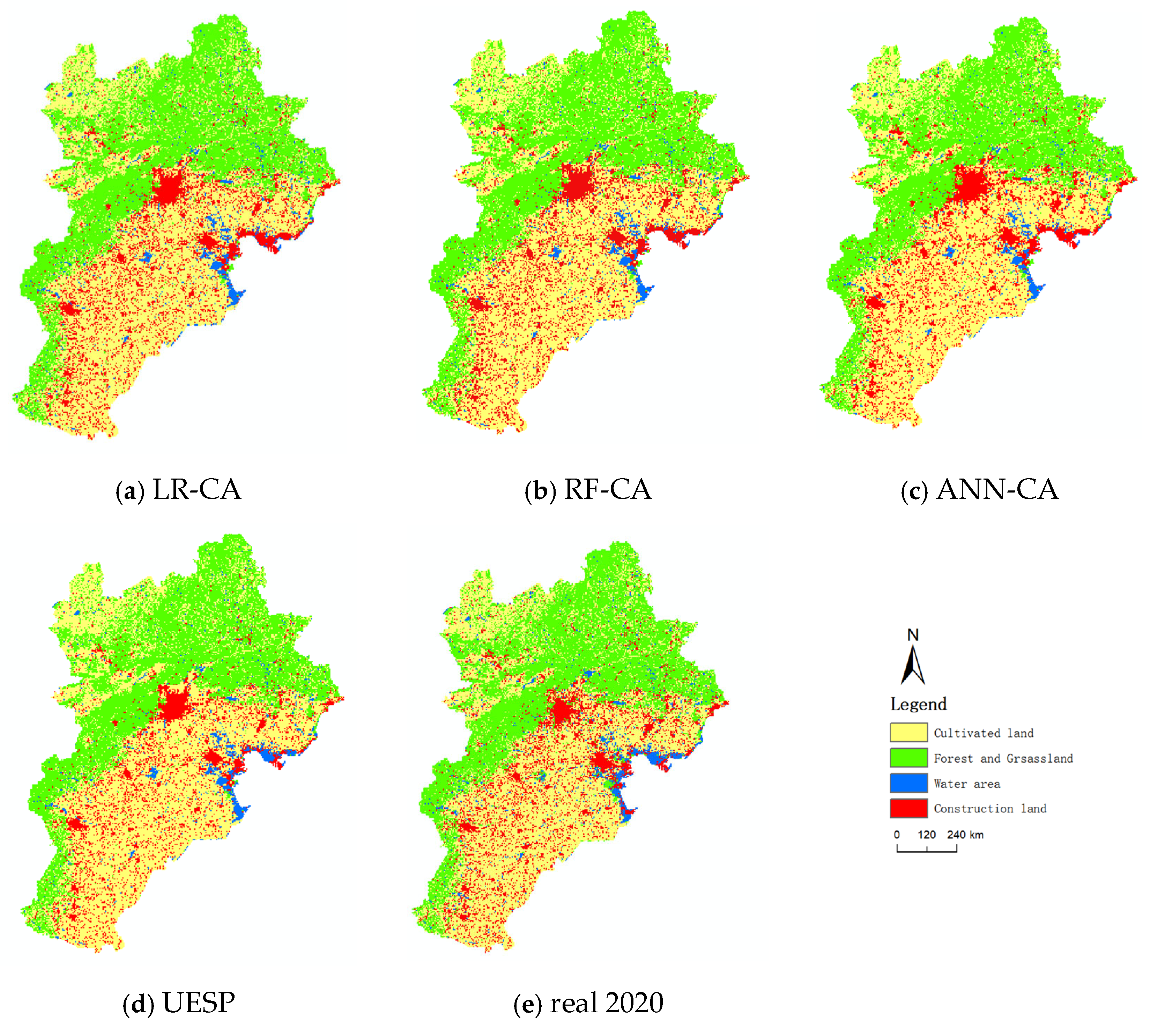
4.1. Application of Model and Results

During model training, the Adam optimizer was used with a learning rate of 0.001 and a training coefficient of 500 epochs. A total of 70% of the sample data from 2000 to 2010 was used for training, while the remaining 30% was reserved for validation to assess the model’s performance. Then, the model’s stability was further evaluated using data from 2010 to 2020. During the training process, dropout (with a dropout rate of 0.6) was applied to mitigate overfitting. Based on previous studies [30], the order of the high-order adjacency matrix for the graph structure was set to k = 2. After multiple iterations, the GAT model with the lowest training loss and best performance was selected as the optimal model. The final test results showed an OA of 0.925 and a Kappa of 0.878, indicating excellent model performance.

The experimental results demonstrate that GAT-VCA effectively captures spatial heterogeneity and neighborhood nonlinear effects, outperforming the traditional CA model (see

Table 3. Comparison results with classical models.

Model	2000–2010			2010–2020
	OA	Kappa	FoM	OA	Kappa	FoM
GAT-VCA	0.89	0.83	0.031	0.901	0.84	0.047
UESP	0.92	0.84	0.036	0.925	0.878	0.048

). Furthermore, the UESP model, enhanced by the integration of the ABM, significantly improves the ability to characterize land use conversion behaviors. The incorporation of micro-level behavioral intentions complements the macro-level structural learning, resulting in a substantial improvement in the model’s simulation accuracy.

In addition, this study also used three other VCA models, namely RF-VCA, LR-VCA, and ANN-VCA, for comparison. Figure 4 illustrates the prediction results of land use change in different models during the simulation process. Based on the visual comparison, the simulation results of the UESP model better reflect the real spatial pattern, although some scattered lands have not been well simulated. The accuracy evaluation results are shown in

Table 4. Simulation results of the accuracy evaluation index based on different models.

Model	OA	PA	UA	FoM	Kappa
LR-VCA	0.867	0.018	0.096	0.015	0.826
RF-VCA	0.915	0.016	0.081	0.013	0.863
ANN-VCA	0.896	0.056	0.111	0.041	0.835
UESP	0.925	0.069	0.162	0.048	0.878

, among which the UESP model has the best simulation effect. The results show that the UESP model is superior to the comparison model in multiple indicators, particularly in the FoM metric, where it improves by 3.5% over RF-VCA, reducing both false positive and false negative rates. It suggests that the model provides higher accuracy in simulating actual land change areas and can more realistically reflect the actual land use evolution process.

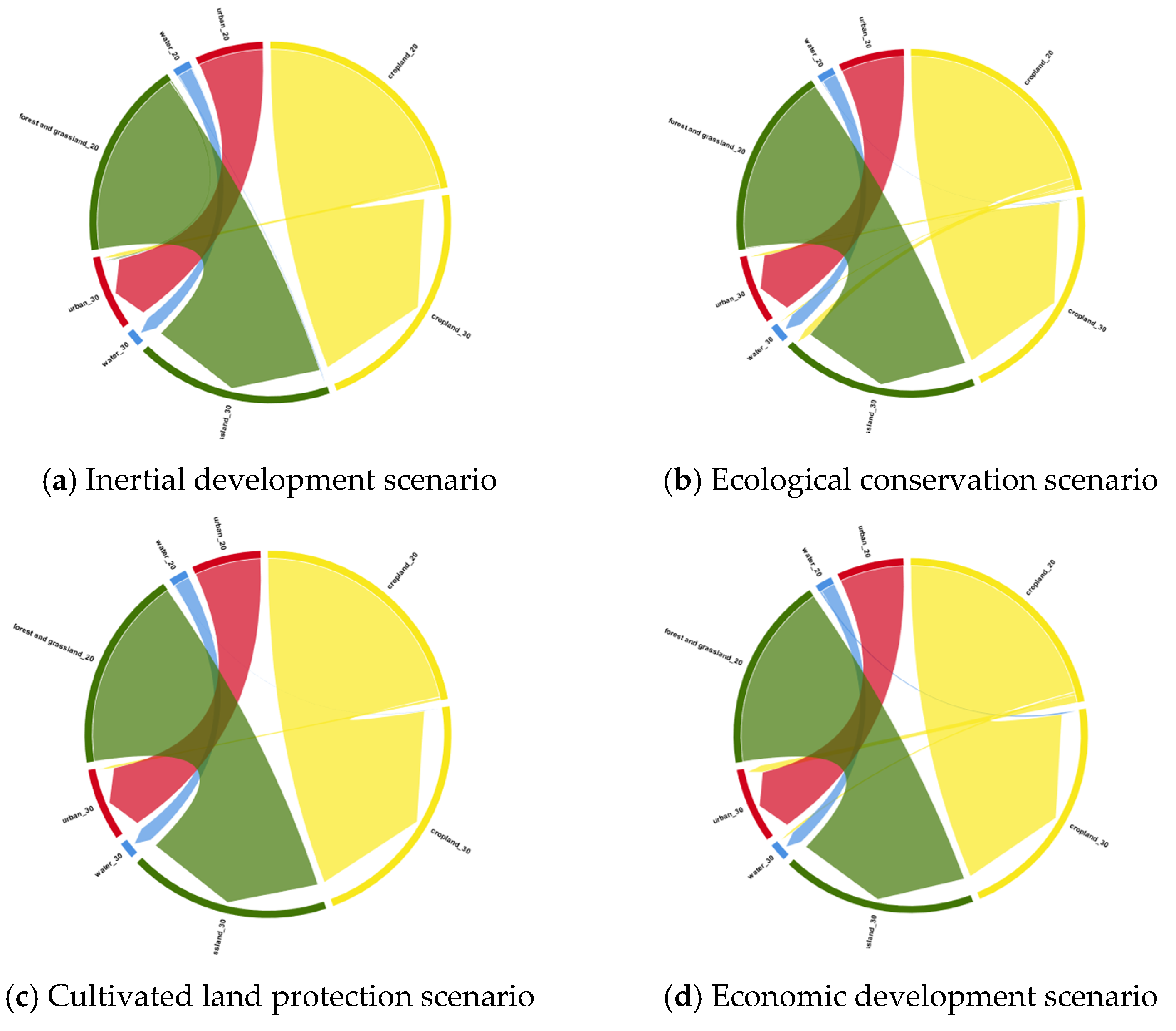
4.2. Future Scenario Simulation

In China, urban development is strongly influenced by government decisions. However, policymaking often entails considerable uncertainty and unpredictability, which poses a great challenge to simulating urban land use change [59]. Based on previous studies and the policy context of the coordinated development of BTH, this paper further designs four scenarios to simulate land use in 2030 using the UESP model [60,61].

Scenario 1: Inertial development scenario. This scenario follows the development direction under the historical trend of the study area, has no strict restrictions on land conversion, excluding the influence of policies and plans, and simulates the land use conversion law from 2010 to 2020.

Scenario 2: Ecological conservation scenario. Combined with the Outline Plan for the Coordinated Development of BTH, the ecological protection belt of the Bashang Plateau and the conservation forest of the Yanshan–Taihang Mountains are classified as restricted conversion areas. According to the land and space planning policies of Beijing, Tianjin, and Hebei Province, water bodies such as rivers and lakes, as well as ecological protection red lines and nature reserves, are set as restricted conversion areas.

Scenario 3: Cultivated land protection scenario. Cultivated land is the land use type with the highest proportion in the study area. Cultivated land security is the key to ensuring regional food security and sustainable development. This scenario sets permanent basic farmland and water areas as restricted conversion areas, reduces the conversion of cultivated land to construction land and forest land, and restricts the conversion of cultivated land to grassland and water areas.

Scenario 4: Economic development scenario. This scenario focuses on the expansion of construction land as the primary objective, reflecting the rapid urban growth trend driven by economic development. Considering the high population density and the substantial water demand for industrial and agricultural activities in BTH, water bodies such as lakes and rivers, ecological redlines, nature reserves, and urban parks are designated as restricted zones where land conversion is prohibited. Other land use types are allowed to be converted to construction land. Additionally, the urban development boundary is applied to constrain the extent of urban expansion.

The simulation results are presented in Figure 5. The pattern and quantity of land use types under each scenario show obvious differences (see

Table 5. Land use quantity in Beijing–Tianjin–Hebei in 2030 under different scenario simulations.

Type of Land Use	Land Use Area (km2)
	2020	Scenario 1	Scenario 2	Scenario 3	Scenario 4
Cultivated land	99,964	98,004	95,104	98,900	94,212
Forest and grassland	81,180	81,136	84,278	81,344	81,256
Water area	7180	6368	7476	6788	7476
Construction land	27,932	30,748	29,400	29,224	33,312

). Cultivated land and forest and grassland are the dominant land use types, comprising 46.22% and 37.54%, respectively.

The trend of land use change under each scenario in the future is as follows:

In scenario 1, large-scale urban expansion occurs around the Beijing–Tianjin metropolitan area, with construction land scattered and widely dispersed. Compared with 2020, the area of construction land increases by 2816 km², primarily at the expense of cultivated land and forest and grassland. It highlights the risks of disorderly urban expansion and ecological degradation in the absence of policy intervention, emphasizing the necessity of coordinated urban planning to achieve a balance between economic growth and environmental protection.

In scenario 2, the ecological conservation policy effectively restrains the expansion of construction land within key ecological zones, resulting in the preservation of forest and grassland. Compared with scenario 1, the forest and grassland area increases by 3142 km², while the construction land decreases by 1312 km². Especially in the ecological protection core area of BTH, forests and grassland are well protected, effectively preventing excessive land development.

In scenario 3, the expansion of cultivated land is effectively safeguarded, and the conversion of cultivated land to construction land, forest land, and grassland is strictly restricted. Compared with scenario 1, the cultivated land area increases by 896 km². Based on guaranteeing cultivated land, the agglomeration development of urban fringe areas is promoted. Urban expansion is projected to primarily occur outward from core cities such as Beijing, Tianjin, Tangshan, Shijiazhuang, Baoding, Xingtai, and Handan.

In scenario 4, under the economic development scenario, the increase in construction land is heavily concentrated in Beijing, Tianjin, Tangshan, and the north, middle, and south regions. In particular, there is a rapid surge in construction land surrounding the capital, which may exacerbate the overload of Beijing’s non-capital function. Compared with 2020, the construction land expands by 5080 km², while the cultivated land decreased by 5753 km², indicating significant ecological pressure under aggressive economic growth.

Through the four scenario simulations and the chord diagram analysis of the land use transfer matrix (see Figure 6), it can be found that the future expansion of construction land in BTH will mainly sacrifice cultivated land, and the urban expansion in the BTH and central and southern Hebei plains is significant, showing a network expansion model of “core driving, axis belt connection, and cluster breakthrough”. BTH will show coordinated development in the future, and the simulation results can provide a scientific basis for different land use planning and sustainable development of urban agglomerations.

5. Discussion

5.1. Analysis of Differences in Simulations of Different Scenarios

As a nationally significant urban agglomeration, the BTH region is a key area for promoting China’s new-type urbanization and regional coordinated development. The BTH Coordinated Development Plan explicitly emphasizes optimizing spatial patterns, strengthening ecological redline controls, facilitating industrial relocation, and relieving the non-capital functions of Beijing, providing clear policy guidance for land use planning.

In this study, simulation experiments were conducted under multiple policy scenarios. The results demonstrate that the UESP model can accurately capture land expansion dynamics under policy constraints and effectively reveal the profound impacts of different policy priorities on land use patterns.

For example, under the “ecological conservation” scenario, construction land is prohibited from expanding within the ecological redline areas, preventing excessive land development and promoting compact growth in the urban fringe. This result is consistent with the findings of Zhang [62], who simulated urban expansion in the Changsha–Zhuzhou–Xiangtan region under an ecological protection scenario and demonstrated that ecological conservation policies can effectively restrict urban growth, significantly slow down expansion rates, and help maintain urban ecological stability. Under the “cultivated land protection” scenario, the control of prime farmland is further strengthened, leading to a greater concentration of construction land in non-agricultural priority areas and safeguarding the security of basic farmland.

By contrast, the “economic development” scenario led to significant urban expansion, particularly the formation of high-density construction clusters around the central areas of Beijing and Tianjin, which exacerbates the challenges associated with large-city syndromes. These variations in spatial distribution under different scenarios illustrate the strong adaptability of the UESP model in simulating policy-responsive urban expansion, providing an effective simulation tool for regional policy evaluation and spatial planning. The simulation outcomes also offer empirical evidence supporting the functional spatial zoning, ecological redline management, and urban growth boundary delineation advocated in China’s National Territorial Spatial Planning Outline (2021–2035).

The results indicate that ecological protection and cultivated land protection policies can significantly suppress disordered urban expansion, improve land use efficiency, enhance and ecosystem stability. In contrast, scenarios driven solely by economic growth tend to intensify urban space expansion, which may lead to ecological degradation and overexploitation of land resources. Therefore, prioritizing ecological improvement, implementing targeted land use optimization strategies, and formulating proactive policy interventions are essential for promoting sustainable and green development in the future.

5.2. Policy Implications

From the perspective of spatial distribution, the main expansion direction of construction land is concentrated in the capital region with Beijing and Tianjin as the core and peripheral node cities such as Langfang and Baoding, forming a belt-shaped aggregation structure of “one core, two cities, and multiple nodes”. This structure not only reflects the spatial integration trend of urban agglomeration development, but also puts forward higher requirements for the decentralization of capital functions and regional coordination.

The future urban expansion and land use patterns of the BTH region will largely depend on scientifically guided policies and the depth of regional cooperation. Based on the results of previous studies and current work, several recommendations are proposed to promote the coordinated and sustainable development of the BTH region:

First, it is essential to strengthen dynamic monitoring and optimize land use structure. By integrating remote sensing monitoring with simulation modeling, the region can continuously assess land use trends and prevent the excessive pursuit of economic growth at the expense of farmland and ecological spaces.

Second, greater emphasis should be placed on ecological construction and the balanced allocation between construction land and ecological land to promote harmonious coexistence between urban development and the ecological environment. It is recommended to reinforce the ecological conservation functions of the northwestern BTH region by continuing key ecological projects such as the Three-North Shelter Forest Program, the Taihang Mountain Afforestation Project, and the Conversion of Cropland to Forest Program to ensure steady progress in ecological restoration.

Third, it is crucial to uphold functional zoning and promote coordinated regional development. The spatial delineation of the ecological conservation zone, functional expansion zone, core functional zone, and coastal development zone in the BTH region should be maintained to ensure balanced growth among different areas. Future development planning should place greater emphasis on ecological priorities, rational industrial distribution, and orderly population management. Through differentiated development strategies, the region can foster functional complementarity, optimize spatial patterns, and achieve high-quality, coordinated development.

5.3. Uncertainty and Limitations

The UESP model integrates macro-level spatial structure modeling, high-order spatial heterogeneity expression, and micro-level individual behavioral simulation, enabling multi-scale and multi-agent coupling for complex urban expansion processes in large urban agglomerations. This framework can effectively support high-precision and policy-adaptive urban expansion simulations. However, it is important to acknowledge that the model has several inherent limitations and sources of uncertainty.

(1)

Policy unpredictability in China:

• In practice, land use policies in China often undergo rapid and unexpected changes. The sudden implementation of environmental redlines, urban renewal projects, or demolition policies can significantly alter urban expansion trends. These abrupt policy shifts are difficult to predict and parameterize within the scenario-based modeling framework.

(2)

Simplified representation of human decision-making:

2.

Although the ABM module incorporates agent-level decision rules, these behaviors are simplified and parameterized using aggregated statistical indicators such as GDP, POI density, and accessibility. Such input variables cannot fully capture the nonlinearity, heterogeneity, and contextual dependence of real human decision-making processes, especially under unexpected social, political, or emergency events (e.g., COVID-19 lockdowns or disaster-induced population migration).

(3)

Limitations of stochastic disturbance factors:

3.

While stochastic factors are incorporated into the CA transition rules to simulate unknown disturbances in the real world, these random disturbances cannot precisely replicate complex, large-scale external shocks such as pandemics or natural disasters. Therefore, the model’s ability to fully represent sudden and highly dynamic environmental changes remains limited.

6. Conclusions

This paper proposed a novel urban expansion scenario prediction model (UESP) that integrates a graph attention network (GAT), vector cellular automata (VCA), and an agent-based model (ABM) to enhance the spatial accuracy and policy adaptability of land use change simulations. The model employs a multi-head attention mechanism to dynamically capture higher-order spatial dependencies of land patches and builds a multi-level simulation framework that combines macro-structural learning with micro-level agent behavior modeling. This approach enables the collaborative simulation of spatial dependencies and individual decision-making processes in urban land use evolution.

The UESP model demonstrated high accuracy and stability in simulating land use change in the BTH region in 2020, achieving an overall accuracy of 92.5%, a Kappa coefficient of 87.8%, and significant improvement in figure of merit (FoM) values compared to traditional models such as LR-VCA, RF-VCA, and ANN-VCA. Furthermore, under the context of the coordinated development policy for the BTH region, four future scenarios—inertial development, ecological conservation, cultivated land protection, and economic growth—were designed and simulated. The results revealed notable differences in urban expansion pathways under varying policy constraints. Specifically, ecological and farmland protection scenarios help mitigate excessive urban sprawl, while a purely economic-driven scenario may exacerbate land pressure and ecological degradation.

This study provides a new modeling approach for multi-source data fusion, high-order spatial heterogeneity representation, and policy-oriented scenario design at the urban agglomeration scale. It also offers scientific insights to support land use planning and sustainable urban development in the BTH region. Due to the limitations of data acquisition, the behavioral modeling of the ABM module is still a static process. Future work could incorporate multi-temporal socioeconomic data, such as population mobility and travel demand, to improve the model’s dynamic responsiveness and adaptability.

References

- Bren, C.; Femke, R.; Giovanni, B.; Stephan, B.; Burak, G.; Eickemeier, K.-H.; Helmut, H.; Felix, C.; Seto, K.C. Future urban land expansion and implications for global croplands. Proc. Natl. Acad. Sci. USA 2016, 114, 8939–8944. [Google Scholar] [CrossRef]
- Seto, K.C.; Güneralp, B.; Hutyra, L.R. Global forecasts of urban expansion to 2030 and direct impacts on biodiversity and carbon pools. Proc. Natl. Acad. Sci. USA 2012, 109, 16083–16088. [Google Scholar] [CrossRef] [PubMed]
- Wei, Y.D.; Ewing, R. Urban expansion, sprawl and inequality. Landsc. Urban Plan. 2018, 177, 259–265. [Google Scholar] [CrossRef]
- Boahen, S.A.; Asante, R.A.; Agyei, G.; Cobbinah, S.B.; Keil, M.; Eltz, S.; Schopp, J.; Schilling, D. Urbanization, land use transformation and spatio-environmental impacts: Analyses of trends and implications in major metropolitan regions of Ghana. Land Use Policy 2020, 96, 104707. [Google Scholar]
- European Commission. The European Green Deal [COM (2019) 640 Final]; European Commission: Brussels, Belgium, 2019. [Google Scholar]
- Chen, M.; Liu, W.; Liu, D. Challenges and the way forward in China’s new-type urbanization. Land Use Policy 2016, 55, 334–339. [Google Scholar] [CrossRef]
- Fang, C. Important progress and future direction of studies on China’s urban agglomerations. J. Geogr. Sci. 2015, 25, 1003–1024. [Google Scholar] [CrossRef]
- Zhu, Z.; He, Q. Spatio-temporal evaluation of the urban agglomeration expansion in the middle reaches of the Yangtze River and its impact on ecological lands. Sci. Total Environ. 2021, 790, 148150. [Google Scholar]
- Wang, Z.; Liu, L.; Shao, Z.; Wu, X. Spatiotemporal differentiation and the factors influencing urbanization and ecological environment synergistic effects within the Beijing-Tianjin-Hebei urban agglomeration. J. Environ. Manag. 2019, 243, 227–239. [Google Scholar] [CrossRef]
- Ma, L.; Liu, Y.; Zhang, X.; Yao, Y.; Yang, G.; Jones, B.A. Deep learning in remote sensing applications: A meta-analysis and review. ISPRS J. Photogramm. Remote Sens. 2019, 152, 166–177. [Google Scholar] [CrossRef]
- Fan, W.; Zhang, S. Urban land expansion in China’s six megacities from 1978 to 2015. Sci. Total Environ. 2019, 664, 60–71. [Google Scholar]
- Chen, W.; Zhang, J.; Li, N. Change in land-use structure due to urbanisation in China. J. Clean. Prod. 2021, 321, 128986. [Google Scholar] [CrossRef]
- Qu, Y.; Liu, H. The economic and environmental effects of land use transitions under rapid urbanization and the implications for land use management. Habitat Int. 2018, 82, 113–121. [Google Scholar] [CrossRef]
- Zhang, Y.; Cheng, W.; Zhang, J. Land-use transfer and its ecological effects in rapidly urbanizing areas: A case study of Nanjing, China. Sustainability 2024, 16, 10615. [Google Scholar] [CrossRef]
- Yu, C.; Zhang, X.; Yang, F.; Liu, Z.; Sun, X. Urban Spatial Growth Modeling Using Logistic Regression and Cellular Automata: A Case Study of Hangzhou. Ecol. Indic. 2020, 113, 106200. [Google Scholar]
- Zhang, H.; Wang, H.; Zhou, B. An Urban Cellular Automata Model Based on a Spatiotemporal Non-Stationary Neighborhood. Int. J. Geogr. Inf. Sci. 2024, 38, 902–930. [Google Scholar] [CrossRef]
- Wu, J.; Makhdoom, M.B.; Dakhil, M.A.A.; Aghajani, M. Machine learning in modelling land-use and land cover-change (LULCC): Current status, challenges and prospects. Sci. Total Environ. 2022, 822, 153559. [Google Scholar]
- Yao, Y.; Liu, X.; Zhang, D.; Liu, Z.; Zhao, Y. Simulation of urban expansion and farmland loss in China by integrating cellular automata and random forest. arXiv 2017, arXiv:1705.05651. [Google Scholar]
- Li, J.; Xu, B.; Liu, Y.; Wang, X.; Bai, Q.; Jiang, J. Simulation of dynamic urban expansion under ecological constraints using a long short term memory network model and cellular automata. Remote Sens. 2021, 13, 1499. [Google Scholar] [CrossRef]
- Haldar, S.; Das, S.; Bera, S. Use of Support Vector Machine and Cellular Automata Methods to Evaluate Impact of Irrigation Project on LULC. Environ. Monit. Assess. 2023, 195, 50. [Google Scholar] [CrossRef]
- Liang, X.; Guan, Q.; Clarke, K.C.; Li, S.; Wang, B.; Yao, Y. Understanding the drivers of sustainable land expansion using a patch-generating land use simulation (PLUS) model: A case study in Wuhan, China. Comput. Environ. Urban Syst. 2020, 85, 101569. [Google Scholar] [CrossRef]
- Guo, J.; Shi, S.; Chen, C.; Duan, K. A Hybrid Spatiotemporal Convolution-Based Cellular Automata Model (ST-CA) for Land-Use/Cover Change Simulation. Int. J. Appl. Earth Obs. Geoinf. 2022, 110, 102789. [Google Scholar]
- Xu, T.; Goh, J.; Cossu, G. Simulation of urban expansion via integrating artificial neural network with Markov Chain–Cellular Automata. Int. J. Geogr. Inf. Sci. 2019, 33, 1960–1983. [Google Scholar] [CrossRef]
- Qi, Y.; Xu, W.; Gao, X.; Yang, T.; Wang, H. Coupling Cellular Automata with Area Partitioning and Spatiotemporal Convolution for Dynamic Land Use Change Simulation. Sci. Total Environ. 2020, 722, 137738. [Google Scholar]
- Wu, Z.; Pan, S.; Chen, F.; Long, G.; Zhang, C.; Yu, P.S. A comprehensive survey on graph neural networks. IEEE Trans. Neural Netw. Learn. Syst. 2021, 32, 4–24. [Google Scholar] [CrossRef]
- Kipf, T.N.; Welling, M. Semi-supervised classification with graph convolutional networks. In Proceedings of the International Conference on Learning Representations, Toulon, France, 24–26 April 2017. [Google Scholar]
- Veličković, P.; Cucurull, G.; Casanova, A.; Romero, A.; Liò, P.; Bengio, Y. Graph attention networks. In Proceedings of the International Conference on Learning Representations, Vancouver, BC, Canada, 30 April–3 May 2018. [Google Scholar]
- Zhang, Y.; Yao, Y.; Gong, Q.; Liu, X.; Li, X.; Peng, Y.; Yu, H.; Yang, Z.; Zhang, J. Simulating urban land use change by integrating a convolutional neural network with vector-based cellular automata. Int. J. Geogr. Inf. Sci. 2020, 34, 1475–1499. [Google Scholar]
- Li, Y.; Chen, M.; Zhang, L. A vector-based cellular automata model for simulating urban land use change. In Proceedings of the 25th International Conference on Geoinformatics, Guangzhou, China, 3–5 January 2014; pp. 74–84. [Google Scholar]
- Guan, X.; Xing, W.; Li, J.; Wu, H. HGAT-VCA: Integrating High-Order Graph Attention Network with Vector Cellular Automata for Urban Growth Simulation. Comput. Environ. Urban Syst. 2023, 99, 101900. [Google Scholar] [CrossRef]
- Li, D.; Zheng, X.; Wang, H. Land-use simulation and decision-support system (LandSDS): Seamlessly integrating system dynamics, agent-based model, and cellular automata. Ecol. Model. 2020, 417, 108924. [Google Scholar] [CrossRef]
- Liu, Y.; Batty, M.; Wu, S.; Corcoran, J. Modelling urban change with cellular automata: Contemporary issues and future research directions. Prog. Hum. Geogr. 2021, 45, 3–24. [Google Scholar] [CrossRef]
- Benenson, I. Agent-Based Models of Geographical Systems. Int. J. Geogr. Inf. Sci. 2013, 27, 1047–1053. [Google Scholar] [CrossRef]
- Li, F.; Li, Z.; Chen, H.; Chen, Z.; Liu, M. An agent-based learning-embedded model (ABM-Learning) for urban land use planning: A case study of residential land growth simulation in Shenzhen, China. Land Use Policy 2020, 95, 104620. [Google Scholar] [CrossRef]
- Crooks, A.; Heppenstall, A.; Malleson, N.; Manley, E. Agent-based modeling and the city: A gallery of applications. In Urban Informatics; Springer: Cham, Switzerland, 2021; pp. 885–910. [Google Scholar]
- Liang, X.; Liu, X.; Li, X.; Xu, X.; Ou, J.; Chen, Y.; Wu, S.; Wang, S.; Pan, F. A future land use simulation model (FLUS) for simulating multiple land use scenarios by coupling human and natural effects. Landsc. Urban Plan. 2017, 168, 94–116. [Google Scholar]
- Liu, Y.; Chen, Y.; Fang, Q.; Zhang, X.; Wang, H.; Yang, Z. Dynamics of Land Use/Land Cover Considering Ecosystem Services for a Dense-Population Watershed Based on a Hybrid Dual-Subject Agent and Cellular Automaton Modeling Approach. Engineering 2024, 37, 182–195. [Google Scholar] [CrossRef]
- Haas, J.; Ban, Y. Urban growth and environmental impacts in Jing-Jin-Ji, the Yangtze River Delta and the Pearl River Delta. Int. J. Appl. Earth Obs. Geoinf. 2014, 30, 42–55. [Google Scholar] [CrossRef]
- National Bureau of Statistics of China. China Statistical Yearbook; China Statistic Press: Beijing, China, 2023. (In Chinese) [Google Scholar]
- Zhou, D.; Wang, C. Specific Evaluation of Resource and Environmental Carrying Capacity of Urbanized Areas for Early-Warning: A Case Study of the Beijing-Tianjin-Hebei Region. Prog. Geogr. 2017, 36, 359–366. (In Chinese) [Google Scholar]
- Yang, J.; Huang, X. The 30m annual land cover datasets and its dynamics in China from 1985 to 2023 [Data set]. Earth Syst. Sci. Data 2024, 13, 3907–3925. [Google Scholar] [CrossRef]
- Al-Kheder, S.; Wang, J.; Shan, J. Fuzzy Inference Guided Cellular Automata Urban-Growth Modelling Using Multi-Temporal Satellite Images. Int. J. Geogr. Inf. Sci. 2008, 22, 1271–1293. [Google Scholar] [CrossRef]
- He, C.; Okata, N.; Zhang, Q.; Shi, P.; Zhou, J. Modeling Urban Expansion Scenarios by Coupling Cellular Automata Model and System Dynamic Model in Beijing, China. Appl. Geogr. 2006, 26, 323–345. [Google Scholar] [CrossRef]
- Lau, K.H.; Kam, B.H. A Cellular Automata Model for Urban Land-Use Simulation. Environ. Plan. B Plan. Des. 2005, 32, 247–263. [Google Scholar] [CrossRef]
- Shen, Q.; Cheng, Q.; Tang, B.; Yung, S.; Huang, Y.; Chiu, G. A System Dynamics Model for the Sustainable Land Use Planning and Development. Habitat Int. 2008, 33, 15–25. [Google Scholar] [CrossRef]
- Qian, S.; Guo, C.J.; Xu, C. Multiple Scenarios Analysis on Land Use Simulation by Coupling Socioeconomic and Ecological Sustainability in Shanghai, China. Sustain. Cities Soc. 2023, 95, 104578. [Google Scholar]
- Wang, F.; Ma, C.; Du, X. Analysis of the Driving Force of Land Use Change Based on Geographic Detection and Simulation of Future Land Use Scenarios. Sustainability 2022, 14, 5254. [Google Scholar] [CrossRef]
- Guan, Q.; Liu, J.; Zhang, Y.; Liu, X.; Yao, Y. HashGAT-VCA: A Vector Cellular Automata Model with Hash Function and Graph Attention Network for Urban Land-Use Change Simulation. Landsc. Urban Plan. 2024, 250, 105145. [Google Scholar] [CrossRef]
- Wu, S.; Sun, F.; Zhang, W.; Xie, X.; Cui, B. Graph Neural Networks in Recommender Systems: A Survey. ACM Comput. Surv. 2023, 55, 97. [Google Scholar] [CrossRef]
- Zhou, J.; Cui, G.; Hu, S.; Zhang, Z.; Yang, C.; Liu, Z.; Wang, L.; Li, C.; Sun, M. Graph Neural Networks: A Review of Methods and Applications. AI Open 2020, 1, 57–81. [Google Scholar] [CrossRef]
- Jiang, W.; Luo, J.; He, M.; Gu, W. Graph Neural Network for Traffic Forecasting: The Research Progress. ISPRS Int. J. Geo Inf. 2023, 12, 100. [Google Scholar] [CrossRef]
- Kumar, V.; Singh, V.K.; Gupta, K.; Jha, A.K. Integrating Cellular Automata and Agent-Based Modeling for Predicting Urban Growth: A Case of Dehradun City. J. Indian Soc. Remote Sens. 2021, 49, 2779–2795. [Google Scholar] [CrossRef]
- Li, S.; Liu, X.; Li, X.; Chen, Y. Simulation Model of Land Use Dynamics and Application: Progress and Prospects. Natl. Remote Sens. Bull. 2017, 21, 329–340. (In Chinese) [Google Scholar] [CrossRef]
- Wibowo, A.; Liu, Y. Cellular Automata for Urban Growth Modelling: A Review on Factors Defining Transition Rules. Int. Rev. Spat. Plan. Sustain. Dev. 2016, 4, 60–75. [Google Scholar]
- Yao, Y.; Liu, L.; Li, Z.; Chen, T.; Shao, Z.; Liu, P.; Guo, Q.; Zhang, Y.; Kong, S.; Chen, Y.; et al. UrbanVCA: A Vector-Based Cellular Automata Framework to Simulate the Urban Land-Use Change at the Land-Parcel Level. arXiv 2021, arXiv:2103.08538. [Google Scholar]
- Liu, D.; Zhang, X.; Zhang, C.; Wang, H. A New Temporal–Spatial Dynamics Method of Simulating Land-Use Change. Ecol. Model. 2017, 350, 1–10. [Google Scholar] [CrossRef]
- Da Cunha, E.R.; Santos, C.A.G.; da Silva, R.M.; Bacani, V.M.; Pott, A. Future Scenarios Based on a CA-Markov Land Use and Land Cover Simulation Model for a Tropical Humid Basin in the Cerrado/Atlantic Forest Ecotone of Brazil. Land Use Policy 2021, 101, 105141. [Google Scholar] [CrossRef]
- Olofsson, P.; Foody, G.M.; Herold, M.; Stehman, S.V.; Woodcock, C.E.; Wulder, M.A. Making Better Use of Accuracy Data in Land Change Studies: Estimating Accuracy and Area and Quantifying Uncertainty Using Stratified Estimation. Remote Sens. Environ. 2013, 129, 122–131. [Google Scholar] [CrossRef]
- Yang, X.; Ling, Y.; Li, L.; Chen, L.; Chen, L. Worst Case Scenario-Based Methodology for Simulating Land-Use Change in Coastal City in China: A Case Study of Lianyungang. Resour. Sci. 2019, 41, 1082–1092. (In Chinese) [Google Scholar]
- Yu, Y.; Yang, M.; Zhang, B.; Liu, Z.; Song, X.; Zhang, Z. Spatially Explicit Carbon Emissions from Land Use Change: Dynamics and Scenario Simulation in the Beijing-Tianjin-Hebei Urban Agglomeration. Land Use Policy 2025, 150, 107473. [Google Scholar]
- Liu, D.; Zhang, X.; Wang, H.; Zhang, C.; Liu, J.; Li, Y. Interoperable Scenario Simulation of Land-Use Policy for Beijing–Tianjin–Hebei Region, China. Land Use Policy 2018, 75, 155–165. [Google Scholar] [CrossRef]
- Fandi, M.; Zhang, Z.; Zhang, P. Multi-Objective Optimization of Land Use in the Beijing–Tianjin–Hebei Region of China Based on the GMOP-PLUS Coupling Model. Sustainability 2023, 15, 3977. [Google Scholar]