Quantifying Ecological Dynamics and Anthropogenic Dominance in Drylands: A Hybrid Modeling Framework Integrating MRSEI and SHAP-Based Explainable Machine Learning in Northwest China

Abstract

Arid and semi-arid regions serve as crucial ecological barriers in China, making the spatiotemporal evolution of their ecological environmental quality (EEQ) scientifically significant. This study developed a Modified Remote Sensing Ecological Index (MRSEI) by innovatively integrating the Comprehensive Salinity Indicator (CSI) into the Remote Sensing Ecological Index (RSEI) and applied it to systematically evaluate the spatiotemporal evolution of EEQ (2014–2023) in Yinchuan City, a typical arid region of northwest China along the upper Yellow River. The study revealed the spatiotemporal evolution patterns through the Theil–Sen (T-S) estimator and Mann–Kendall (M-K) test, and adopted the Light Gradient Boosting Machine (LightGBM) combined with the Shapley Additive Explanation (SHAP) to quantify the contributions of ten natural and anthropogenic driving factors. The results suggest that (1) the MRSEI outperformed the RSEI, showing 0.41% higher entropy and 5.63% greater contrast, better characterizing the arid region’s heterogeneity. (2) The EEQ showed marked spatial heterogeneity. High-quality areas are concentrated in the Helan Mountains and the integrated urban/rural development demonstration zone, while the core functional zone of the provincial capital, the Helan Mountains ecological corridor, and the eastern eco-economic pilot zone showed lower EEQ. (3) A total of 87.92% of the area (7609.23 km²) remained stable with no significant changes. Notably, degraded areas (934.52 km², 10.80%) exceeded improved zones (111.04 km², 1.28%), demonstrating an overall ecological deterioration trend. (4) This study applied LightGBM with SHAP to analyze the driving factors of EEQ. The results demonstrated that Land Use/Land Cover (LULC) was the predominant driver, contributing 41.52%, followed by the Digital Elevation Model (DEM, 18.26%) and Net Primary Productivity (NPP, 12.63%). This study offers a novel framework for arid ecological monitoring, supporting evidence-based conservation and sustainable development in the Yellow River Basin.

1. Introduction

With global climate change and intensified human activities, the ecological environment in arid and semi-arid areas is facing increasingly serious challenges, such as the food crisis [1], land desertification [2], the decline in biodiversity [3], and other prominent problems. China places ecological conservation at the core of its green development strategy, following the sustainable development principle that “lucid waters and lush mountains are invaluable assets”. As a critical ecological barrier in China, the arid northwest region plays a key role in implementing major national ecological projects, including the “Two Barriers and Three Belts” ecological security pattern and the “Northern Sand Control Belt” initiative. Accurate assessment of ecological quality status and its temporal dynamics in China’s arid and semi-arid regions is crucial for enhancing ecological governance and regional planning [4]. However, existing studies overlook critical environmental stressors like soil salinization. This limitation reduces the accuracy of ecological quality quantification and driver analysis in these regions. To address this gap, we innovatively developed the Modified Remote Sensing Ecological Index (MRSEI), which enables a comprehensive dynamic assessment of ecological quality in fragile ecosystems. By incorporating explainable machine learning techniques, our approach enhances understanding of the underlying driving mechanisms. This study establishes a novel methodological framework for regional ecological quality assessment. It also offers new perspectives for tackling global environmental challenges and advancing ecological sustainability.

Ecological quality evaluation is a systematic process and serves as a key indicator for measuring the livability of a region. It provides a fundamental basis for resource development, sustainable socio-economic planning, and ecological protection strategies [5]. Currently, ecological environment assessments are primarily categorized into two approaches. The first relies on a single indicator for evaluation [6,7]. However, ecological environmental quality (EEQ) represents a complex integration of internal structures and external states [8]. Given the intricate relationships among its components, a single indicator is insufficient to accurately reflect the overall condition of a regional ecosystem. The second approach is based on integrated indicators, with the Remote Sensing Ecological Index (RSEI) being a representative example [9]. This index utilizes NDVI, WET, LST, and NDBSI as input variables and applies principal component analysis (PCA) to determine their weights objectively. In contrast to single-indicator analysis, PCA objectively assigns weights to each component, thereby rendering the RSEI more comprehensive and unbiased. Consequently, the RSEI has been widely adopted for ecological monitoring across various spatial scales [10,11,12]. However, while the RSEI effectively characterizes urban ecological conditions, its application in arid and semi-arid regions often overlooks critical ecological issues such as soil salinization. This omission is particularly significant, as soil salinization reduces soil permeability and water infiltration capacity, potentially exacerbating desertification processes [13]. As a result, these limitations may compromise the accuracy of EEQ in such environments. To address these issues, some researchers have developed improved versions of the RSEI by adding or substituting remote sensing indicators tailored to the ecological characteristics of arid and semi-arid regions. For example, Wang et al. [14] added a land degradation index (LDI) to the RSEI to quantitatively evaluate the ecological quality of arid zones. Although the model considered the common problem of soil salinity in arid and semi-arid zones, the LDI reflected land cover changes and failed to directly quantify soil salinity, which is the core ecological problem in arid zones. Moreover, the synergistic mechanism between salinization and vegetation degradation was not sufficiently analyzed, making it difficult to distinguish between natural degradation and the impacts of anthropogenic activities. In another study, Wang et al. [15] developed a modified RSEI (MRSEI) by replacing the dryness index with a salinity index (SI) and adding an air quality index (DI) to support EEQ monitoring and prediction in the Yellow River Delta. However, this modified framework exhibited a critical limitation: the absence of a dedicated dryness indicator to characterize surface aridification. Since dryness metrics directly reflected land surface drought conditions [16], this omission resulted in an incomplete assessment of ecological quality in arid and semi-arid regions.

Currently, remote sensing technology has become an effective tool for monitoring and identifying soil salinity levels [17]. Salinity indices are routinely used to characterize soil salt content, thereby enabling indirect assessment of EEQ in arid and semi-arid regions [18]. In soil salinity research, the Normalized Difference Salinity Index (NDSI) has been shown to provide high measurement accuracy, making it particularly suitable for quantifying salinization in dryland areas [17]. Furthermore, in sparsely vegetated regions, the combined application of the NDSI and the Thermal-based Salinity Index (SI-T) has demonstrated superior performance in salinity assessment [19]. To overcome the limitations of using a single salinity index to capture the complex environmental dynamics of soil salinization in arid and semi-arid regions, this study introduced a Comprehensive Salinity Index (CSI) integrating both the NDSI and SI-T. Building upon this foundation, we innovatively proposed the MRSEI, designed to comprehensively capture both surface-apparent and subsurface-latent characteristics of salinization. This methodological advancement provides theoretical support for monitoring and combating ecological degradation in dryland ecosystems. Yinchuan, located in the transitional zone between arid and semi-arid regions in northwest China, is a key central city and a representative dryland area in the Ningxia Plain along the upper reaches of the Yellow River. The local ecological environment is strongly disturbed by urbanization, industrial and agricultural activities, leading to vegetation degradation, soil salinization, and sanding. Therefore, this study employed the MRSEI to assess the EEQ in Yinchuan. This not only reflects the regional characteristics of dryland ecosystems in northwest China but also supports the formulation of targeted ecological conservation and restoration strategies.

In arid and semi-arid regions, the EEQ is affected by a combination of climate, elevation, socio-economic factors, and other factors. Common approaches used in the study of driving mechanisms include grey prediction models (GM) [20,21], geographically weighted regression (GWR) [22,23], and geographical detectors (GD) [24,25]. However, GM relies on small sample data sizes and does not account for spatial heterogeneity, making it unsuitable for modeling high-dimensional nonlinear relationships or capturing localized differences in driver effects [26]. GWR, while capable of handling spatial variation, is limited to fitting linear or partially linear relationships and assumes independence between natural and anthropogenic factors. This assumption fails to capture the complex nonlinear interactions among variables and their influence on EEQ [27,28]. While GD can detect interactions between factors, it cannot distinguish between the positive and negative effects of drivers [29,30,31]. In recent years, machine learning has played a crucial role in data mining, image recognition, and natural language processing due to its powerful computational capacity. It is widely applied to mine complex non-linear relationships between independent and dependent variables [32]. To enhance the interpretability and reliability of our model predictions, we incorporated SHAP (Shapley Additive Explanations), an interpretable machine learning method based on game theory’s Shapley values. SHAP quantifies the contribution of each feature to model predictions and provides both global and local model interpretations, facilitating a better understanding of model behavior [33,34]. Therefore, this study used machine learning combined with SHAP to comprehensively explore the importance of key driving factors, the intensity of interaction effects, and non-linear functional relationships, offering a novel perspective on the driving mechanisms of EEQ.

In summary, this study took Yinchuan City as the research area. Based on the Google Earth Engine (GEE) platform and combined with multi-source remote sensing data from 2014 to 2023, the EEQ in arid and semi-arid regions was dynamically assessed using the MRSEI. The spatiotemporal variation of EEQ in Yinchuan was further examined using the T-S estimator and M-K test. Based on the SHAP explainable machine learning model, ten key driving factors—encompassing both natural and anthropogenic variables—were identified and analyzed to uncover the primary influences on EEQ in the study area. This study introduces a novel MRSEI capable of precisely characterizing EEQ in arid and semi-arid regions. By employing explainable machine learning techniques, the study quantitatively reveals the positive and negative impacts of various ecological drivers, as well as their interaction effects. This approach addresses a long-standing limitation of traditional approaches in quantifying individual feature contributions. The proposed methodology offers a novel perspective and practical solution for EEQ assessment in arid and semi-arid regions, while providing critical scientific references for ecological conservation and sustainable development strategies in northwestern Chinese cities. The findings not only enhance our understanding of EEQ dynamics in arid and semi-arid ecosystems but also serve as valuable references for regional ecological management and policy-making.

2. Study Area and Datasets

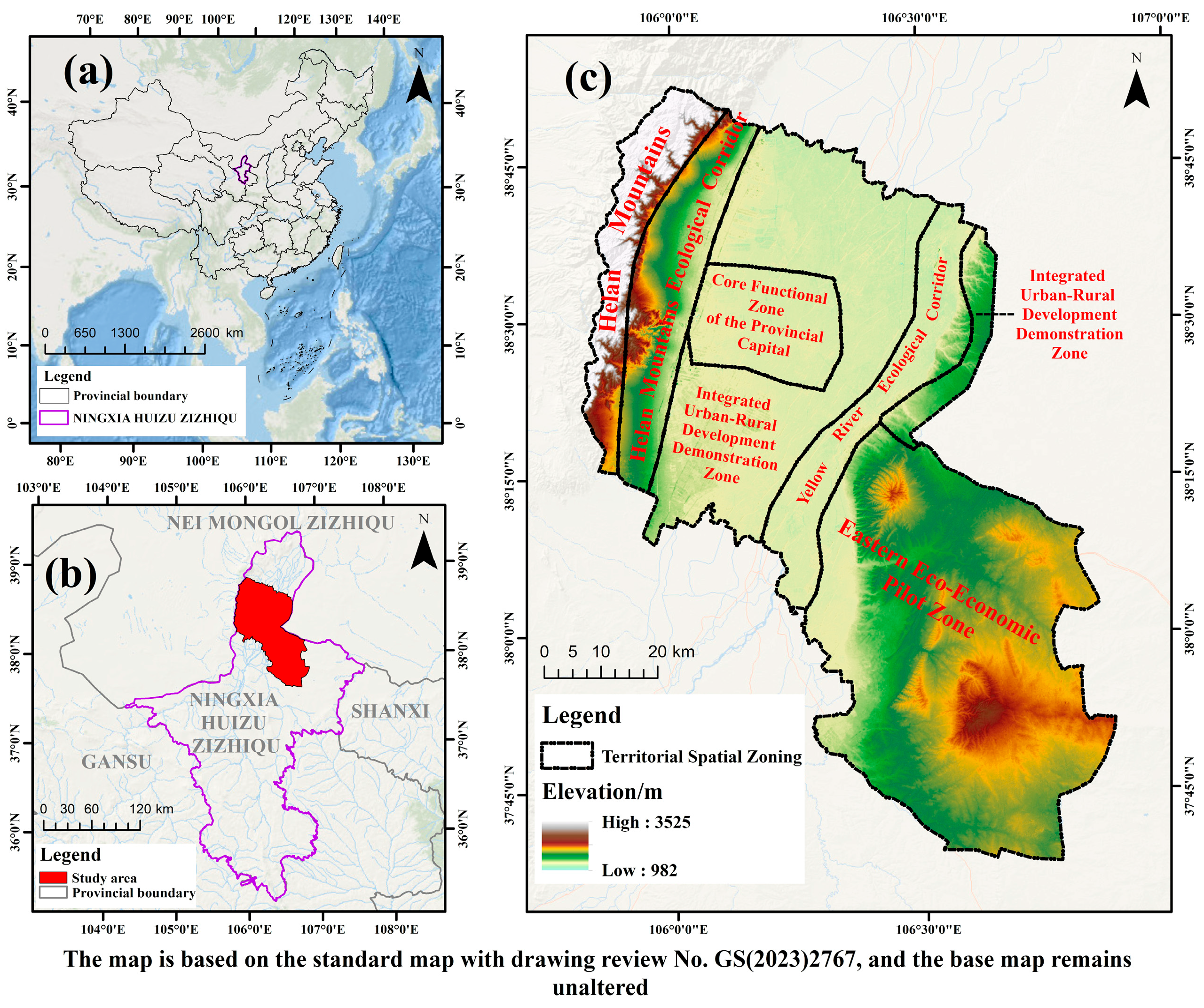
2.1. Study Area

Yinchuan (38°08′N–39°23′N, 105°49′E–106°35′E) is located in the upper reaches of the Yellow River, bordered by the Helan Mountains to the west, adjacent to the Alxa League of Inner Mongolia, with Wuzhong City to the south and Shizuishan City to the north (Figure 1). The city covers a total area of 9025.38 km², with elevations ranging from 982 to 3525 m. The terrain is divided into two major parts: mountainous regions and plains. The western and southern parts are relatively elevated, whereas the northern and eastern areas lie at lower altitudes. Yinchuan exhibits a typical temperate continental semi-arid climate, with an annual mean temperature of approximately 8.5 °C and a mean annual precipitation of around 200 mm, predominantly occurring during summer months. Land use in Yinchuan City is predominantly agricultural, and the area is rich in wetland resources. In this study, the zoning scheme defined in the Yinchuan Territorial Space Master Plan (2021–2035) was adopted to partition the study area for subsequent analysis (Figure 1).

2.2. Datasets

This study incorporates multi-source datasets spanning from 2014 to 2023, including remote sensing imagery, topographic data, and socio-economic statistics (

Table 1. Data source.

Data Type	Data Name	Spatial Resolution	Source
RSEI/MRSEI	LANDSAT8 OLI	30 m	https://developers.google.com
	MOD11A2	1 km	https://developers.google.com
anthropogenic drivers	POP	1 km	https://landscan.ornl.gov
	NTL	1 km	https://dataverse.harvard.edu
	GDP	1 km	https://www.resdc.cn
	LULC	30 m	https://doi.org/10.5281/zenodo.4417809
natural drivers	PRE	1 km	https://data.tpdc.ac.cn/home
	TEM	1 km	https://data.tpdc.ac.cn/home
	VPD	1 km	https://data.tpdc.ac.cn/home
	DEM	1 km	https://www.resdc.cn/
	SLO	1 km	https://www.resdc.cn/
	NPP	1 km	https://www.resdc.cn/

). The remote sensing data were obtained from Landsat 8 OLI and MODIS MOD11A2 products accessed through GEE, featuring spatial resolutions of 30 m and 1000 m, respectively. All datasets underwent radiometric calibration, geometric correction, and atmospheric correction. Nearest-neighbor interpolation was applied to resample the imagery to a consistent spatial resolution of 30 m, facilitating long-term time-series analysis. As this study focuses on EEQ, the imagery was selected from July to September when vegetation coverage is typically at its peak. To ensure data reliability, all selected imagery maintained cloud cover below 10%. On the GEE platform, cloud masking was performed using the QA band from Landsat imagery, and images from adjacent months were used to fill data gaps. Furthermore, to minimize potential interference from water bodies on the RSEI calculations, we applied a water mask derived from the China Land Cover Dataset (CLCD) to exclude large water areas. In analyzing the driving factors of the MRSEI, this study systematically selected ten determinants encompassing both natural and anthropogenic dimensions. The anthropogenic factors include (1) population density (POP), (2) nighttime light intensity (NTL), (3) land use/land cover (LULC), and (4) gross domestic product (GDP). The natural factors comprise (1) Digital Elevation Model (DEM), (2) slope gradient (SLOPE), (3) cumulative precipitation (PRE), (4) mean air temperature (TMP), (5) vapor pressure deficit (VPD), and (6) net primary productivity (NPP). To ensure consistency across all variables, we resampled all datasets to a uniform spatial resolution of 30 m.

3. Methods

The overall framework of this research is illustrated in Figure 2.

3.1. MRSEI Model

The RSEI is an ecological evaluation index constructed by selecting the first principal component through PCA using the normalized vegetation index (NDVI), bare soil index (NDBSI), moisture index (WET), and temperature index (LST) as indicators [9]. Building upon the traditional RSEI framework, this study introduces an ensemble learning-based enhancement by incorporating a Comprehensive Salinity Index (CSI)—calculated as the arithmetic mean of the SI-T [4] and NDSI [35]—to construct the MRSEI. This modification aimed to improve the accuracy of EEQ assessments in arid and semi-arid regions. The following formula is used to calculate the MRSEI:

$$MRSEI=f\left(NDVI,WET,CSI,NDBSI,LST\right)$$

(1)

where NDVI is the normalized vegetation index [36], WET is the humidity component of the tasseled cap transformation [37], CSI is the composite salinity index obtained from the mean of SI-T and NDSI, and NDBSI is a synthesis of the bare soil index SI and the building index IBI [38].

To ensure temporal consistency and stability in the LST component, the study utilized the MODIS LST product (MOD11A2) [4], which provides 8-day composite thermal infrared data at a spatial resolution of 1 km. Detailed formulas for each individual remote sensing ecological indicator used in this study are provided in

Table 2. Calculation of each Remote Sensing Ecological Index.

Index	Calculation
NDVI	$NDVI=\left({\rho }_{nir}-{\rho }_{red}\right)/\left({\rho }_{nir}+{\rho }_{red}\right)$
WET	${WET}_{TM}=0.0315{\rho }_{blue}+0.2021{\rho }_{green}+0.3012{\rho }_{red}+0.1594{\rho }_{nir}-0.6806{\rho }_{SWIR1}-0.6109{\rho }_{SWIR2}$ ${WET}_{OLI}=0.1511{\rho }_{blue}+0.1973{\rho }_{green}+0.3283{\rho }_{red}+0.3407{\rho }_{nir}-0.7117{\rho }_{SWIR1}-0.4559{\rho }_{SWIR2}$
NDBSI	$NDBSI=\left(IBI+SI\right)/2$ $IBI={\displaystyle \frac{2{\rho }_{swir1}/({\rho }_{swir1}+{\rho }_{nir})-[{\rho }_{nir}/({\rho }_{nir}+{\rho }_{red})+{\rho }_{green}/({\rho }_{green}+{\rho }_{swir1})}{{2\rho }_{swir1}/({\rho }_{swir1}+{\rho }_{nir})+[{\rho }_{nir}/({\rho }_{nir}+{\rho }_{red})+{\rho }_{green}/({\rho }_{green}+{\rho }_{swir1})}}$ $SI={\displaystyle \frac{\left({\rho }_{swir1}+{\rho }_{red}\right)-({\rho }_{nir}+{\rho }_{blue})}{\left({\rho }_{swir1}+{\rho }_{red}\right)+({\rho }_{nir}+{\rho }_{blue}}}$
CSI	$CSI=(SI-T+NDSI)/2$ $SI-T={\displaystyle \frac{{\rho }_{red}}{{\rho }_{nir}}}\times 100$ $NDSI={\displaystyle \frac{\left({\rho }_{red}-{\rho }_{nir}\right)}{\left({\rho }_{red}+{\rho }_{nir}\right)}}$

.

To standardize the measurement scales across all MRSEI components and prevent weighting bias caused by dimensional heterogeneity, we normalized the five indices (NDVI, WET, CSI, NDBSI, and LST) to a uniform [0, 1] range using min/max normalization. The normalization formula is expressed as:

$$N{I}_i=\left(I_i-I_{min}\right)/\left(I_{max}-I_{min}\right)$$

(2)

where $N{I}_i$ is the normalized ecological index value, $I_i$ is the original ecological index value, $I_{max}$ is the maximum image value of this ecological index, and $I_{min}$ is the minimum image value of this ecological index.

The normalized five ecological indices were integrated using PCA, with the first principal component (PC1) serving as the initial value for the MRSEI, as expressed by the following formula:

$$MRSE{I}_0=P{C}_1\left[f\left(NDVI,WET,NDBSI,LST,CSI\right)\right]$$

(3)

where $f\left(·\right)$ is the PCA operation, $P{C}_1\left[f\left(·\right)\right]$ denotes taking the PC1, and $MRSE{I}_0$ is the initial value of MRSEI.

For standardized measurement and comparative analysis, the initial MRSEI₀ values were normalized to the MRSEI using the following min-max transformation:

$$MRSEI=\left(MRSE{I}_0-MRSE{I}_{0min}\right)/\left(MRSE{I}_{0max}-MRSE{I}_{0min}\right)$$

(4)

where $MRSE{I}_0$ is the initial value of MRSEI; $MRSE{I}_{0min}$ and $MRSE{I}_{0max}$ are the minimum and maximum values of $MRSE{I}_0,$ respectively.

3.2. Spearman’s Rank Correlation Analysis

Spearman’s rank correlation analysis is a non-parametric statistical method used to assess the strength and direction of a monotonic relationship between two variables by ranking the data values. This method is particularly effective in identifying statistically significant monotonic associations between the MRSEI and potential environmental driving factors, regardless of the underlying distribution of the data. The Spearman’s rank correlation coefficient ($\rho$) is calculated as:

$$\rho =1-{\displaystyle \frac{6\sum _{i=1}^n{d}_i^2}{n(n^2-1)}}$$

(5)

where n is the number of samples; $d_i$ is the difference in rank of each sample i on the two variables.

3.3. T-S Estimator and M-K Test

The T-S estimator and M-K test are two commonly used non-parametric statistical methods [39], which offer the advantages of not requiring a specific distribution and being unaffected by outliers [40]. In this study, the T-S estimator was first applied to quantify the magnitude and direction of long-term trends in the MRSEI, followed by the M-K test to evaluate the statistical significance of these trends [41]. This approach has been widely adopted in assessing long-term ecological quality trends [42].

The T-S estimator is calculated by the formula:

$$\beta =median\left({\displaystyle \frac{x_j-x_i}{j-i}}\right),\forall j>i$$

(6)

where median is the median function, $x_i$, and $x_j$ represent the value of year i and year j, respectively; this study refers to the MRSEI of the year i and year j, β > 0 represents the upward trend, β < 0 represents the downward trend.

The M-K test is calculated by the formula:

$$S={\sum }_{i=1}^{n-1}{\sum }_{j=i+1}^{n}sgn\left(x_j-x_i\right)$$

(7)

$$sgn\left(x_j-x_i\right)=\left\{\begin{array}{c} 1, x_j-x_i>0 \\ 0, x_j-x_i=0\\ -1, x_j-x_i<0\end{array}\right.$$

(8)

The formula for the standardized test statistic Z is as follows:

$$Z=\left\{\begin{array}{c}{\displaystyle \frac{S-1}{\sqrt{VAR\left(S\right)}}}, S>0\\ 0 , S=0\\ {\displaystyle \frac{S+1}{\sqrt{VAR\left(S\right)}}}, S<0\end{array}\right.$$

(9)

where S is the test statistic and $\sqrt{VAR\left(S\right)}$ is the variance of S; Z is the standardized test statistic.

In this study, when |Z| ≥ 1.96, the trend is considered statistically significant at the 95% confidence level, while |Z| ≥ 2.58 indicates significance at the 99% confidence level. Following the trend categories from similar studies [40], the trend levels are categorized as shown in

Table 3. Trend categories.

Trend	Significance	Trend Type	Trend Feature
Slope > 0	|Z| > 2.58	ESI	Extremely significant improvement
	1.96 < |Z| ≤ 2.58	SI	Significant improvement
	|Z| ≤ 1.96	NSC	No significant change
Slope < 0	|Z| ≤ 1.96	NSC	No significant change
	1.96 < |Z| ≤ 2.58	SD	Significant degradation
	|Z| > 2.58	ESD	Extremely significant degradation

.

3.4. Machine Learning

3.4.1. Machine Learning Models

Machine learning identifies patterns and underlying rules from large-scale datasets through algorithmic optimization by minimizing loss functions, thereby enabling effective prediction and classification of unseen data [43]. In recent years, machine learning has been extensively applied across various domains and has demonstrated significant potential in ecological remote sensing research [44]. This study selected 10 driving factors from both natural and anthropogenic aspects and employed seven machine learning models—Random Forest (RF), eXtreme Gradient Boosting (XGBoost), Adaptive Boosting (AdaBoost), Categorical Boosting (CatBoost), Light Gradient Boosting Machine (LightGBM), Least Absolute Shrinkage and Selection Operator (Lasso), and Gradient Boosting (GradientBoosting)—to construct the MRSEI driving force model. Since the driving factors and MRSEI in this study exhibit time-series characteristics, the training set was partitioned using the TimeSeriesSplit method [45].

RF is an ensemble learning model based on decision trees (DTs) classifiers, and is widely used for both classification and regression tasks [46]. XGBoost employs decision or regression trees as base learners and incorporates explicit regularization terms into the objective function to control model complexity, effectively mitigating the risk of overfitting [47]. The core mechanism of AdaBoost lies in its iterative training of multiple weak classifiers while dynamically adjusting sample weights according to the classification performance of each iteration, ultimately aggregating the results into a strong classifier through a weighted voting strategy [48]. CatBoost is characterized by its symmetric tree structure, which significantly enhances training and prediction efficiency while reducing memory consumption [49]. LightGBM adopts a leaf-wise growth strategy to optimize performance, demonstrating superior capabilities in handling high-dimensional data with lower memory usage and faster model convergence [50]. LASSO is a regularized linear regression technique that introduces an L1 penalty term (i.e., the sum of the absolute values of model coefficients) into the loss function, thereby achieving coefficient shrinkage, feature selection, and overfitting prevention [51]. The core concept of Gradient Boosting involves iteratively improving the model by minimizing the loss function through gradient descent [52].

3.4.2. Evaluation of Model Indicators

The estimation accuracy and predictive capability of machine learning models were evaluated using the coefficient of determination (R²), root mean square error (RMSE), and mean absolute error (MAE). R² measures the goodness-of-fit of the model, with values closer to 1 indicating higher predictive accuracy. RMSE and MAE quantify the error between predicted and observed values, where lower values signify superior model performance. The calculation formulas for R², RMSE, and MAE are as follows:

$$R^2=1-{\displaystyle \frac{RSS}{TSS}}=1-{\displaystyle \frac{{\sum }_{i=1}^N{\left({\widehat{y}}_i-y_i\right)}^2}{{\sum }_{i=1}^N{\left(y_i-{\overline{y}}_i\right)}^2}}$$

(10)

$$RMSE=\sqrt{{\displaystyle \frac{1}{N}}{\sum }_{i=1}^N{\left({\widehat{y}}_i-\overline{y}\right)}^2}$$

(11)

$$MAE={\displaystyle \frac{1}{N}}$$

(12)

where N represents the number of samples, RSS denotes the residual sum of squares, TSS indicates the total sum of squares, $y_i$ is the observed value, ${\widehat{y}}_i$ corresponds to the predicted value, and $\overline{y}$ signifies the mean of observed values.

3.4.3. Interpretable Machine Learning SHAP Models

The SHAP model is a powerful interpretability framework designed to explain the output of machine learning models by computing Shapley values, which quantify the individual contribution of each feature to a specific prediction [53]. It facilitates both global and local interpretability of model decisions [54], offering insights into the internal logic of otherwise “black-box” algorithms. For any given sample, the Shapley value ${\varnothing }_i$ of feature parameter i is calculated as follows:

$${\varnothing }_i={\sum }_{S\subseteq N\backslash \left(i\right)}{\displaystyle \frac{\left|S\right|M-\left|S\right|-1!}{M!}}\left\{f_x\left[S\cup \left(i\right)\right]-f_{x}S\right\}$$

(13)

where N represents the complete set of feature parameters with M total dimensions, S denotes a specific subset selected from N characterized by its dimensionality |S|, and $f_{x}S$ provides the predictive result generated using only the feature subset S. The function $f_x\left[S\cup \left(i\right)\right]$ generates outputs by incorporating parameter i into the existing feature subset S. The magnitude of the Shapley value reflects the degree of influence exerted by the feature parameter on model predictions. A positive Shapley value indicates a positive contribution to the prediction, while a negative value signifies an adverse effect.

4. Results

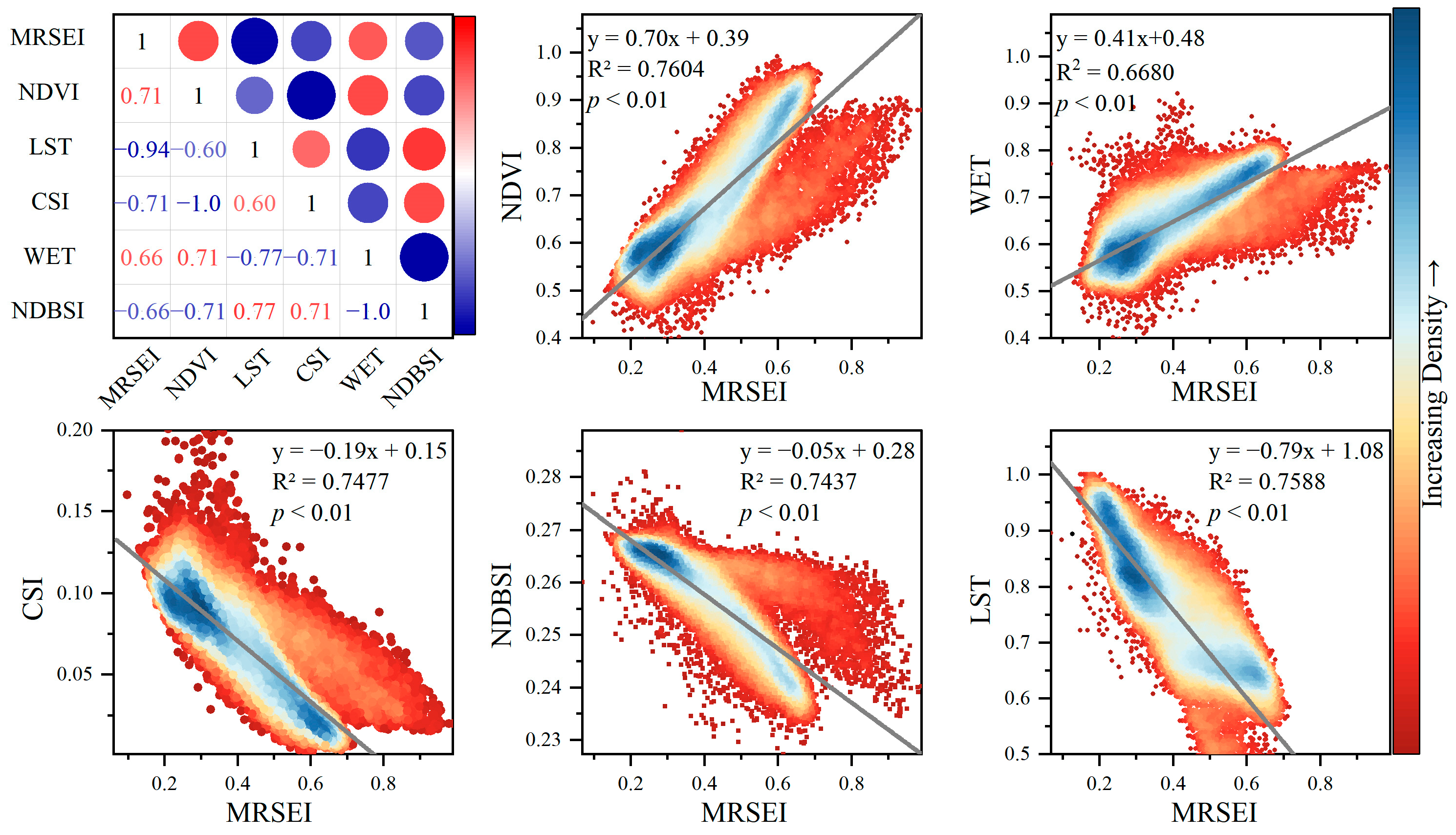
4.1. Effectiveness of the MRSEI

PCA is a dimensionality reduction technique that efficiently condenses multi-band information into fewer transformed bands, with the majority of the original information concentrated in the first principal component (PC1) [9].

Table 4. The statistics of the first principal component loadings and contribution rates of the five ecological indicators.

PC1	NDVI	WET	CSI	NDBSI	LST	Percentage Variance
2014	0.6578	0.2456	−0.1152	−0.0052	−0.7026	81.82
2015	0.6643	0.1785	−0.2451	−0.0156	−0.6830	82.94
2016	0.5045	0.2544	−0.0008	−0.3658	−0.7395	77.43
2017	0.5812	0.2249	−0.1851	−0.0478	−0.7583	81.49
2018	0.5813	0.2287	−0.1342	−0.0017	−0.7693	75.6
2019	0.5836	0.3004	−0.0102	−0.0245	−0.7539	79.49
2020	0.6340	0.2204	−0.0768	−0.0313	−0.7366	82.7
2021	0.5673	0.1799	−0.0698	−0.0213	−0.8003	84.85
2022	0.6075	0.3590	−0.1629	−0.0443	−0.6881	74.51
2023	0.6158	0.2727	−0.0475	−0.0123	−0.7376	78.72

presents the loadings and contribution rates of PC1 for the five MRSEI-integrated ecological indicators. The contribution rate of PC1 exceeded 74.51%, with an average contribution rate reaching 79.96%, indicating that PC1 retained the majority of the ecological information derived from the five indices. These results confirm that PC1 captures the essential characteristics of the five component indicators—NDVI, WET, CSI, NDBSI, and LST—and can effectively represent the local ecological environment. The NDVI and WET, which are positively correlated with ecological quality, exhibited consistent positive loadings, whereas the CSI, NDBSI, and LST, which are negatively correlated, showed consistent negative loadings that were opposite in sign to those of the NDVI and WET [55]. This opposite pattern of loadings aligns with ecological theory and further demonstrates the validity and robustness of the MRSEI in capturing ecological quality variations.

To examine the correlations between individual indicators and the MRSEI, we conducted Spearman’s rank correlation analysis for the year 2022. The results demonstrated significant correlations between all evaluated indicators and the MRSEI (Figure 3). Specifically, the absolute values of correlation coefficients among the indicators ranged from 0.66 to 0.94, indicating strong correlations, and all indicators passed the significance test at p < 0.01. Notably, the newly introduced CSI exhibited a significant negative correlation with the MRSEI, further enriching the explanatory power of the indicator system for the EEQ. In terms of directional relationships, the NDVI and WET showed significant positive correlations with the MRSEI, and the high MRSEI values were primarily concentrated in the high-value zones of these two indicators. This result confirms that vegetation coverage and surface moisture positively contribute to regional EEQ. Conversely, the CSI, NDBSI, and LST exhibited significant negative correlations with the MRSEI, indicating that soil salinization, surface bareness, and land surface temperature exert clear negative impacts on the EEQ. These findings provide important quantitative evidence for regional EEQ and identify key regulatory factors for guiding ecological restoration strategies.

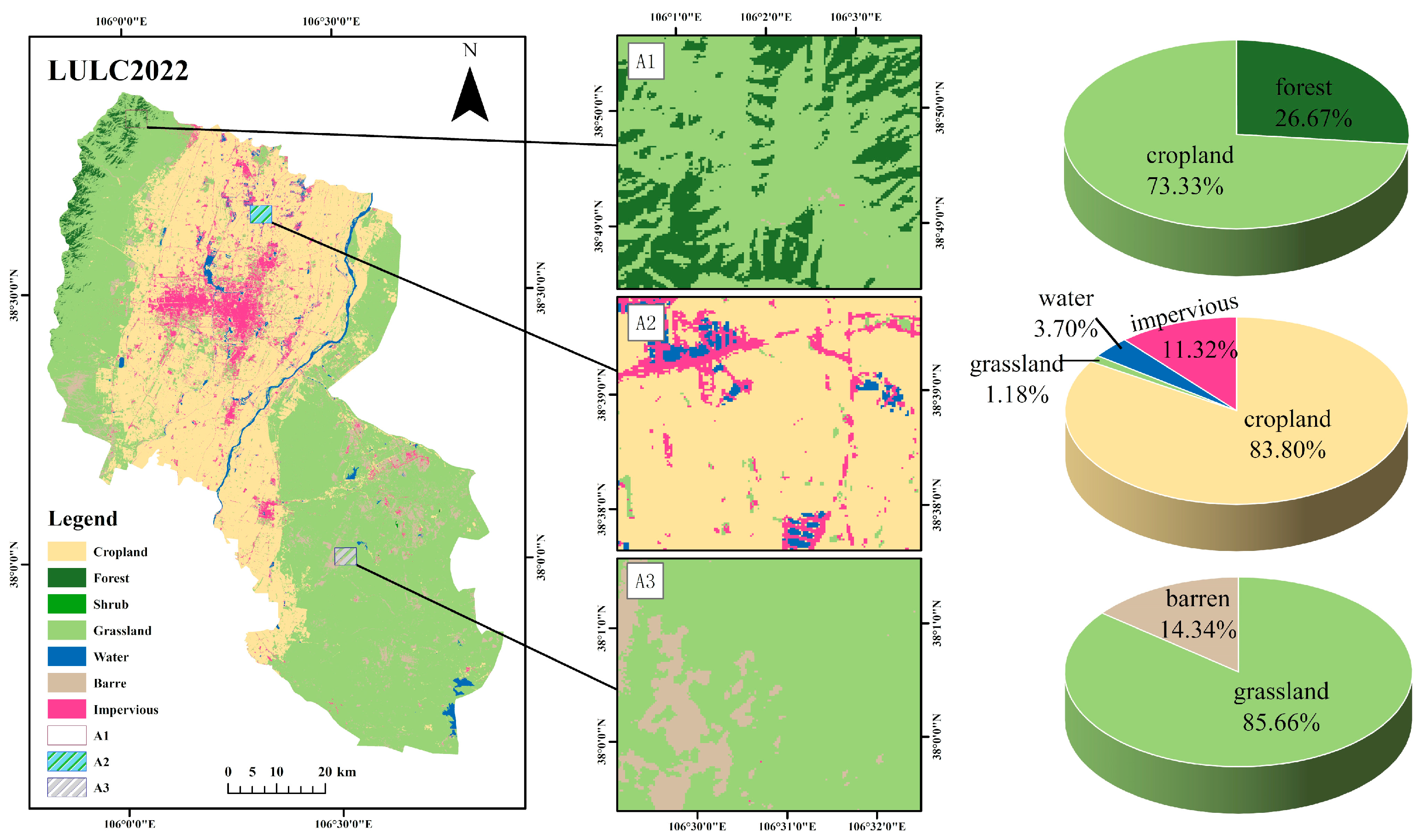
4.2. Applicability of the MRSEI

To evaluate the consistency in overall trends and the differences in spatial distribution between the MRSEI and RSEI in assessing regional ecological environment quality, this study selected three representative test areas in 2022, each exhibiting distinct land cover characteristics. A comparative analysis was conducted from two perspectives: spatial distribution differences and contrast/entropy metrics. Contrast and entropy were introduced as dimensionless parameters to quantify image quality. Contrast reflects the sharpness of an image and the depth of texture grooves; higher values indicate finer texture and clearer visual effects, while lower values suggest more blurred results. Entropy measures the amount of information contained in an image. An increase in entropy implies greater complexity or heterogeneity in texture distribution, reflecting richer spatial detail. Figure 4 shows the selected typical regions shows that A1 is predominantly covered by dense vegetation, A2 is mainly characterized by urban built-up areas, and A3 primarily features desert and sparse grassland.

Based on the 2022 LULC data of Yinchuan, spatial differences among the three typical test areas were comparatively analyzed (Figure 5). In Area A1, the RSEI and MRSEI values were 0.3828 and 0.3987, respectively. The MRSEI exhibited enhanced local texture details in forest and grassland areas, providing a more accurate representation of the actual ecological conditions. In Area A2, the RSEI and MRSEI values were 0.5729 and 0.5816, respectively. The RSEI exhibited a fragmented representation of croplands, whereas the MRSEI provided a more coherent delineation of agricultural patterns, achieving better agreement with actual surface conditions. In Area A3, which exhibited evident signs of soil salinization and desertification, the MRSEI demonstrated higher sensitivity in identifying the distribution and boundaries of barren and grassland areas. Compared with the RSEI, the MRSEI showed better consistency between ecological classification levels and actual land use types. This improvement is attributed to the incorporation of the CSI, which enhances the detection of salinized and decertified areas. In summary, the MRSEI offers a more accurate and reliable assessment of EEQ, reflecting spatial heterogeneity more faithfully than the traditional RSEI.

To more precisely quantify the differences between the RSEI and MRSEI in capturing land cover diversity and complexity, this study calculated their entropy and contrast using the Gray-Level Co-occurrence Matrix (GLCM) on the GEE platform, as presented in

Table 5. The contrast and entropy values for both the entire study area and typical sub-regions.

		Yinchuan	A1	A2	A3
Entropy	RSEI	3.7704	4.1532	4.1215	3.6921
	MRSEI	3.7859	4.1588	4.1237	4.0912
	MRSEI-RSEI	0.0155	0.0056	0.0021	0.3992
Contrast	RSEI	55.1548	491.5241	715.6769	87.9047
	MRSEI	58.2594	536.3671	851.7575	143.6763
	MRSEI-RSEI	3.1046	44.8430	136.0806	55.7716

. Statistical analysis indicated that the MRSEI outperformed the RSEI in both entropy and contrast. For the entire study area, the MRSEI exhibited a higher entropy value by 0.0155 (a 0.41% increase) and a greater contrast value by 3.1046 (a 5.63% increase), indicating its superior capability in preserving information content and capturing fine-scale spatial details. Particularly in Areas A2 and A3, the MRSEI showed more pronounced improvements over the RSEI. These results highlight that the incorporation of the CSI enhances the model’s sensitivity to textural variation across different land cover types, thereby more effectively representing ecosystem complexity and spatial heterogeneity.

4.3. Characteristics of Spatial and Temporal Changes in Ecological Quality

4.3.1. Spatial Distribution Characteristics of the MRSEI

Based on the GEE platform, we constructed the MRSEI for Yinchuan City from 2014 to 2023. As shown in Figure 6, the MRSEI values primarily ranged between 0.15 and 0.60, with median values fluctuating between 0.30 and 0.50 across most years, indicating notable temporal variability in ecological quality. To assess the EEQ spatially, the MRSEI was classified into five levels based on the equal interval method commonly adopted in previous studies [4,9,56]: Poor (0–0.2), Fair (0.2–0.4), Moderate (0.4–0.6), Good (0.6–0.8), and Excellent (0.8–1.0). The graded MRSEI maps for 2014–2023 (Figure 7) reveal a pronounced spatial heterogeneity in EEQ across Yinchuan City, characterized by a general trend of “higher ecological quality in the northwest and lower in the southeast”. The high-quality ecological zones were primarily concentrated in two typical regions: (1) the Helan Mountains in western Yinchuan, and (2) the integrated urban/rural development demonstration zone. In contrast, relatively poorer ecological quality was observed in the core functional zone of the provincial capital, the Helan Mountains ecological corridor, and the eastern eco-economic pilot zone. This spatial pattern underscores the detrimental impacts of intensive human activity, soil salinization, and low vegetation coverage on regional EEQ. An integrated analysis combining MRSEI results with LULC maps further demonstrated that regions categorized as “Excellent”, “Good”, and “Moderate” were largely composed of cropland and forest, while areas dominated by impervious surfaces and low-vegetation grasslands were associated with “Fair” and “Poor” ecological conditions. During 2014–2023, the ecological quality along the Yellow River basin generally maintained a relatively high level, with most areas falling into the “Good” category. However, this region exhibited a notable decline over time, as evidenced by a decrease in “Good” areas and a corresponding increase in “Moderate” zones. This degradation primarily resulted from intensified human activities, including extensive land-use changes—particularly agricultural expansion—which have driven progressive ecosystem degradation. Notably, during 2016 (Figure 7c), 2019 (Figure 7f), and 2021 (Figure 7h), the ecological quality exhibited patchy degradation patterns, primarily occurring in the Helan Mountains ecological corridor and eastern eco-economic pilot zone. These grassland-dominated areas experienced degradation due to the combined effects of climate change, anthropogenic disturbances, and water resource management practices [56,57].

4.3.2. Temporal Distribution Characteristics of the MRSEI

Visualization of MRSEI grade proportions in Yinchuan City (2014–2023) (Figure 8) reveals significant dynamic changes in ecological quality across the study area. Temporally, the MRSEI mean values exhibited a distinct “W”-shaped fluctuation pattern, peaking in 2015 (0.4649), declining to 0.3671 in 2016, recovering to a secondary peak in 2017 (0.4443), then dropping to 0.3764 in 2019, rising again to 0.4343 in 2020, and finally, reaching the study period’s minimum in 2021 (0.3665). A comprehensive analysis of the MRSEI grade composition indicated that Yinchuan City was predominantly characterized by “Fair” and “Moderate” ecological quality levels during this decade. In contrast, the proportions of “Good” and “Excellent” grades remained relatively low, with the “Excellent” grade showing stable proportions year-to-year. The “Poor” grade, however, exhibited notable increases in 2016, 2019, and 2021, corresponding with the lowest points in the MRSEI time series. To clarify transitions between ecological quality grades, we generated Sankey diagrams of the MRSEI grade transfer matrices for Yinchuan City (2014–2023) (Figure 8b). These diagrams reveal that the “Excellent” grade maintained high stability, while frequent transitions occurred among “Fair”, “Moderate”, and “Good” grades. These mutual conversions between adjacent grades likely represented the primary driver of MRSEI fluctuations. Notably, recurrent fluctuations between “Fair” and “Poor” ecological quality grades were observed in 2016, 2019, and 2021, demonstrating a characteristic annual transition pattern, downgrading from “Fair” to “Poor” followed by subsequent upgrading back to “Fair” the following year. This distinct grade alternation showed significant coupling with phased MRSEI declines, suggesting potential threshold responses in ecological quality induced by climatic variability or intensive anthropogenic disturbances.

Analysis of MRSEI grade area statistics (

Table 6. MRSEI grade area statistics (km²).

	Poor	Fair	Moderate	Good	Excellent
2014	1.26	4840.82	2183.98	1585.89	48.48
2015	0.78	4303.52	2300.17	2019.89	41.83
2016	370.37	5016.77	2771.34	473.66	32.15
2017	0.84	4317.70	2808.68	1464.31	71.76
2018	1.53	4569.42	3245.58	762.99	72.10
2019	379.65	4901.68	2594.50	732.65	46.54
2020	0.10	4448.28	2699.92	1448.89	49.27
2021	1200.92	3945.34	2622.73	847.67	38.69
2022	183.78	4773.28	2762.33	895.54	43.28
2023	297.96	4686.68	2549.46	1083.56	36.66

) and annual grade variation trends (Figure 9) for Yinchuan City (2014–2023) provides a clear visualization of ecological quality dynamics. Overall, distinct areal shifts were observed among the different ecological quality grades during the study period. The areas classified as “Excellent”, “Good”, and “Fair” exhibited decreasing trends, with annual rates of change of –0.95 km²/yr, –64.23 km²/yr, and –16.56 km²/yr, respectively. In contrast, the “Moderate” and “Poor” categories showed increasing trends, expanding at rates of 29.12 km²/yr and 51.39 km²/yr, respectively. Specifically, the “Excellent” grade reached a notable peak (72.10 km²) in 2018 (Figure 9a), marking the highest level during the study period. Sankey diagram analysis indicates that this increase was predominantly driven by transfers from the “Moderate” grade. The “Good” grade exhibited a sharp decline in 2016 (Figure 9b), primarily attributed to the transition of partial “Good” areas to “Moderate” grades in 2015. The “Moderate” grade showed an overall increasing trend (Figure 9c), peaking at 3245.58 km² in 2018, followed by a slight decline while remaining at relatively high levels thereafter. The “Fair” grade demonstrated a “W”-shaped fluctuation pattern (Figure 9d), with alternating periods of recovery and decline, though it ultimately showed an overall downward trend. The “Poor” grade experienced rapid expansions during 2016, 2019, and 2021 (Figure 9e), reaching a maximum area of 1200.92 km² in 2021. These expansions were primarily driven by large-scale transitions from “Fair” grade areas, underscoring episodes of marked ecological deterioration. In summary, the significant decreases in MRSEI mean values during 2016, 2019, and 2021 were closely associated with both the expansion of “Poor” grade areas and the reduction of “Good” grade areas, highlighting periods of intensified ecological degradation in Yinchuan City.

4.4. Trend Analysis of Ecological Quality

Based on the T-S estimator and M-K test, this study quantified and visualized the spatial/temporal trends of MRSEI changes in Yinchuan City from 2014 to 2023. The spatial distribution of MRSEI trends (Figure 10) reveals that ecological improvement areas were predominantly concentrated in the integrated urban/rural development demonstration zone. This positive trend showed a significant correlation with local government-led ecological restoration projects, including water-saving irrigation promotion, farmland ecological transformation, and wetland conservation initiatives [56]. In contrast, the ecological environment quality of the Helan Mountain ecological corridor, characterized by dense vegetation and minimal anthropogenic disturbance, remained largely stable throughout the study period. Notably, degraded areas exhibited a distinct “severe in southeast, mild in northwest” spatial pattern, with the most pronounced degradation occurring in the Yellow River ecological corridor and eastern eco-economic pilot zone. As illustrated by the land use distribution map of Yinchuan City (Figure 7), extensive expansion of impervious and cropland in the Yellow River corridor has been a major driver of ecological degradation. Human activity disturbances and intensified land development during rapid urbanization, particularly urban expansion along the Yellow River, have reduced the area of natural grasslands, leading to the destruction of the natural ecological environment and degradation of ecological functions on both banks of the Yellow River. Relevant departments should continue to strengthen ecological protection measures in the Yellow River basin. This deterioration trend originated from intensified anthropogenic disturbances during rapid urbanization and increased land development intensity, particularly the urban expansion along the Yellow River that caused natural ecosystem fragmentation and ecological function degradation [58]. MRSEI trend classification statistics (

Table 7. Area statistics of MRSEI trend grades.

Trend Type	Area (km2)	Proportion
ESI	21.1959	0.24%
SI	89.8398	1.04%
NSI	7609.2300	87.92%
SD	790.6590	9.14%
ESD	143.8580	1.66%

) revealed that from 2014 to 2023, the ecological quality in Yinchuan City was predominantly characterized by “NSC”, covering 7609.23 km² (87.92% of the study area). The total improved areas accounted for 1.28%, comprising “ESI” (21.1959 km², 0.24%) and “SI” (89.8398 km², 1.04%). Degraded areas represented 10.80%, including “ESD” (143.8580 km², 1.66%) and “SD” (790.6590 km², 9.14%). Overall, the degraded areas substantially exceeded the improved areas, indicating a general ecological deterioration trend in Yinchuan City during 2014–2023. Relevant departments should adopt locally specific measures, continue to protect the Helan Mountain ecological corridor, strengthen the governance and restoration of the Yellow River basin, rationally plan the utilization of land resources, and safeguard the ecological environment.

4.5. Analysis of the Driving Factors of the MRSEI

4.5.1. Comparison of Machine Learning Models

To systematically identify the key drivers underlying the spatial heterogeneity of the MRSEI, this study selected ten representative driving factors based on a coupled natural–human system framework. The natural factors comprised six indicators: topography (DEM, SLOPE), climate (PRE, TMP, VPD), and vegetation productivity (NPP). The human factors included four indicators: POP, NTL, LULC, and GDP. A 1 km × 1 km fishnet sampling grid was established, with 4349 samples per year, resulting in a total of 43,490 spatial samples across the study period. For the categorical variable LULC, label encoding was applied to transform each land use category into a unique numerical identifier, enabling compatibility with machine learning algorithms. To enhance driving force analysis precision, this study developed an ensemble modeling framework incorporating seven machine learning algorithms: RF, XGBoost, AdaBoost, CatBoost, LightGBM, Lasso, and Gradient Boosting. The performance of these models was rigorously evaluated using three commonly adopted metrics: R², MAE, and RMSE.

The comparative evaluation results (

Table 8. Comparison of machine learning model performance metrics.

	R2	MAE	RMSE
RF	0.6873	0.0603	0.0751
XGBoost	0.6721	0.0619	0.0773
AdaBoost	0.6728	0.0617	0.0769
CatBoost	0.6838	0.0607	0.0759
LightGBM	0.6918	0.0596	0.0746
Lasso	0.4285	0.0821	0.1021
GradientBoosting	0.6881	0.0597	0.0749

) identified LightGBM as the optimal model, achieving the highest predictive accuracy with an R² of 0.6918, the lowest MAE (0.0596), and the lowest RMSE (0.0746). These results underscore LightGBM’s superior capability in capturing the complex nonlinear interactions between natural and anthropogenic drivers influencing MRSEI spatial patterns.

4.5.2. Interpretable Machine Learning Model Analysis

To systematically quantify the contributions of individual driving factors to ecological quality in Yinchuan City, this study integrated the LightGBM model with SHAP for feature interpretability. The feature importance ranking analysis (Figure 11) revealed LULC as the most influential factor (41.52%, SHAP value = 0.073), significantly exceeding other drivers. DEM (18.26%, SHAP = 0.0321) and NPP (12.63%, SHAP = 0.0222) ranked second and third, respectively. These three factors collectively accounted for 74.41% of total contributions, representing dominant MRSEI drivers. Human factors (53.41%) slightly outweighed natural factors (46.59%), confirming the characteristic dual-system (“natural–human”) synergy governing ecological quality in Yinchuan. The SHAP dependence plots (Figure 12) further elucidate nonlinear response mechanisms of driving factors: (1) LULC exhibited wide-ranging SHAP values (−0.15 to 0.20), indicating substantial variability in impact intensity across different land use types; (2) SLOPE demonstrated consistently low-magnitude influence (−0.02 to 0.03); (3) DEM showed significant negative association with the MRSEI (SHAP values concentrated in negative range), while NPP displayed distinct positive driving effects (SHAP values clustered in positive range), revealing an ecological antagonism between topographic constraints and vegetation productivity enhancement.

To further clarify the driving mechanisms underlying the MRSEI dynamics, this study conducted a statistical analysis of annual driver contributions, as shown in Figure 13. Despite interannual variations, LULC, DEM, and NPP consistently emerged as the dominant contributors to MRSEI variation throughout the study period. The temporal analysis revealed a characteristic anthropogenic/natural synergistic mechanism, with nearly balanced contribution ratios (approximately 50% each). These findings reaffirm LULC, DEM, and NPP as the primary driving factors shaping the spatial–temporal heterogeneity of the MRSEI in Yinchuan City from 2014 to 2023.

This study further explored the mechanistic effects of the three dominant driving factors—LULC, DEM, and NPP—on the MRSEI in Yinchuan City, revealing clear threshold responses in their ecological impacts, as illustrated in Figure 14. The results showed that (1) LULC exhibited significant land-class heterogeneity in its impacts (Figure 14). Among them, the SHAP values of cropland and forest were centrally distributed in the positive SHAP interval, with a peak value close to 0.1, indicating stable enhancement effects on the MRSEI; on the contrary, the SHAP values of grassland, water, barren, and impervious surfaces were mostly located in the negative interval, with a minimum of about −0.1, revealing their suppressive influence on ecological quality. (2) DEM exhibited distinct elevation threshold effects (Figure 14). A positive SHAP value cluster occurred in the 1100–1150 m altitudinal zone, while values showed negative dispersion above 1150 m, reflecting both ecological degradation risks and enhanced spatial heterogeneity in high-elevation areas. (3) NPP displayed a distinct ecological productivity threshold (Figure 14). When NPP values were below 175 g C/m²/yr, SHAP values formed dense negative clusters, transitioning to positive values above this threshold with progressively wider distributions. This pattern indicated a shift from inhibitory to enhancing effects on the MRSEI with increasing NPP, accompanied by growing variability in impact magnitude.

SHAP interaction dependence analysis was employed to reveal how feature interactions influenced LightGBM model outputs. A SHAP value of zero indicated no interactive effect, while positive or negative values represented enhancing or inhibiting interactions, respectively. To investigate these interactions, this study focused on the three dominant drivers—LULC, DEM, and NPP—and analyzed their pairwise interactive effects on the MRSEI (Figure 15). As illustrated in Figure 15a, when NPP was below 175 g C/m²/yr, higher DEM values exhibited stronger inhibitory effects on the MRSEI. In contrast, when NPP exceeded 175 g C/m²/yr, lower DEM values demonstrated significant positive effects. Figure 15b reveals that at elevations below 1140 m, cropland and grassland positively enhanced the MRSEI, while above this threshold, cropland, grassland, and impervious surfaces suppressed the MRSEI. Figure 15c shows that when NPP was less than 175 g C/m²/yr, cropland, grassland, and impervious surfaces displayed stronger suppression, but when NPP surpassed this threshold, cropland and grassland contributed positively. Overall, areas characterized by NPP > 175 g C/m²/yr and DEM < 1140 m consistently showed higher MRSEI values. These results demonstrate the existence of complex, non-linear interactions among environmental variables, where their combined effects on ecological quality are highly dependent on topographic conditions, vegetation productivity, and land use patterns.

5. Discussion

5.1. Ecological Environment Quality Assessment

Currently, the RSEI is widely applied in urban ecological environment assessments [9]. However, ecological quality evaluation requires region-specific adaptations due to varying environmental characteristics across different areas. Yinchuan City, located in the central Ningxia Plain along the upper Yellow River in China’s arid northwest, represents a typical arid and semi-arid ecosystem. Existing RSEI-based ecological assessments in Yinchuan [56] have often failed to sufficiently account for key ecological challenges such as soil erosion and salinization, potentially undermining the reliability of evaluation outcomes. Salinity plays a crucial role in regulating vegetation growth, soil moisture dynamics, and land surface temperature in salinized areas, thereby influencing all core components of the RSEI [59]. Soil salinization, a major form of land degradation, is one of the most severe environmental issues affecting arid and semi-arid zones. In recent years, researchers have developed numerous salinity indices (e.g., $S{I}_1-S{I}_6$, NDSI, SI-T) based on the spectral characteristics of soil salinity to directly assess soil salt content [60,61]. Among these, the SI-T has been introduced into the RSEI to better capture salinity effects, and studies have demonstrated that integrating the SI-T improves the RSEI’s applicability to arid and semi-arid regions through principal component analysis (PCA) and correlation-based evaluations [62]. In the context of Yinchuan City, several studies have confirmed the high accuracy of the NDSI in detecting soil salinity when compared to other indices [63]. However, due to variations in soil genesis conditions, parent materials, salt composition, and the interaction mechanisms between salt and soil particles, the spectral responses of salinized soils differ substantially between regions. As a result, relying on a single salinity index is insufficient for robust and accurate quantification [60,64]. To address this limitation, the present study proposes the CSI, computed by averaging SI-T and NDSI, and subsequently incorporated CSI into an improved MRSEI framework to enhance both the robustness and stability of salinization assessments [4]. This study evaluates the applicability of the MRSEI in arid and semi-arid regions using various methods such as PCA, calculating the eigenvector directionality of the five indicators, comparing texture features of remotely sensed images, and calculating the contrast and entropy, etc. Compared with previous studies [65,66], this research not only qualitatively compares the MRSEI’s spatial distribution patterns but also quantitatively evaluates its advantages by computing contrast and entropy metrics for both the entire study area and representative sub-regions. The results indicated that PC1 explained over 74.51% of the total variance, with an average contribution rate of 79.96%, confirming that PC1 effectively captured and integrated the ecological information contained in the five indicators, consistent with earlier findings [66]. Among the components, the NDVI and WET positively influenced ecological quality, whereas the CSI, LST, and NDBSI exhibited negative effects, aligning with empirical observations and theoretical expectations [9]. By comprehensively addressing soil salinization, the MRSEI has proved more suitable for regional ecological assessments in arid and semi-arid regions [4]. The MRSEI-based evaluation of Yinchuan City’s ecological quality from 2014 to 2023 revealed a distinct spatial pattern of “higher in the northwest, lower in the southeast”. Temporally, MRSEI values exhibited significant “W”-shaped fluctuations, reflecting dynamic ecological changes over the decade. To further assess ecological quality trends, the T-S estimator and Mann–Kendall (M-K) test were applied, revealing that “No Significant Change” was the dominant trend (7609.23 km²), which is consistent with prior findings [56,67]. Notably, Yinchuan City has significantly enhanced regional ecosystem stability and ecological barrier functions through a series of large-scale ecological projects. These include windbreak and sand-fixation forests on the Helan Mountains and the Ordos Plateau, farmland shelterbelt systems, and water conservation forest initiatives. Particularly important are the restoration activities in ecologically fragile areas such as the eastern Yellow River sandy grasslands and the Helan Mountain region. Among these, farmland ecological transformation projects promoted by municipal authorities have played a pivotal role in improving environmental quality, especially within the urban–rural integrated development demonstration zones [56].

5.2. Analysis of Ecological Environment Driving Mechanisms

In exploring the driving mechanisms of the MRSEI, machine learning approaches have demonstrated clear advantages over traditional methods such as Geographically Weighted Regression [68,69] and Geographical Detectors [70,71], particularly in their ability to capture complex, nonlinear interactions between natural and anthropogenic factors and ecological quality. These advanced models enable a more nuanced analysis of factor-specific positive and negative contributions, thereby offering deeper mechanistic insights into MRSEI dynamics. Previous studies have employed Random Forests (RF) to identify landscape ecological risk factors and quantify their relative importance [72]. The advent of SHAP has significantly advanced driver analysis, enabling both global and local interpretation of feature contributions. This approach has been widely adopted, exemplified by CatBoost-SHAP frameworks used to analyze spatiotemporal variations in ecological and socio-economic drivers in Diqing Prefecture [49], and by comparative assessments of RF, GBDT, and XGBoost models combined with SHAP for soil organic carbon prediction [73]. Building upon these advancements, this study developed an ensemble framework incorporating seven machine learning models—RF, XGBoost, AdaBoost, CatBoost, LightGBM, Lasso, and GradientBoosting—to investigate the driving forces of the MRSEI. Model performance was comprehensively evaluated using R², MAE, and RMSE metrics, and the optimal model was selected based on its predictive accuracy, thereby mitigating single-model bias and enhancing result robustness. The results identified LULC, DEM, and NPP as the dominant factors influencing ecological quality in Yinchuan City from 2014 to 2023, underscoring the synergistic effects of natural and anthropogenic drivers, consistent with previous studies [15,74,75]. Among land use types, cropland and forest exerted primarily positive influences on the MRSEI. Elevations between 1100 and 1150 m significantly enhanced ecological quality, while increasing NPP values above 175 g C/m²/yr were associated with a progressively improved MRSEI. Comprehensively, forested areas were predominantly associated with NPP > 175 g C/m²/yr, and in such high-NPP environments, cropland and grassland with dense vegetation cover contributed positively to ecological quality. This positive contribution was more pronounced in areas with DEM < 1140 m, suggesting that land use planning and protection efforts should prioritize cropland in low-elevation regions. According to the 14th Five-Year Plan for Ecological and Environmental Protection in Yinchuan City, strategic priorities include safeguarding the soil environmental quality of cultivated land, delineating the boundaries of ecological security zones, promoting systematic governance and ecological restoration of the Yellow River basin, and strengthening conservation efforts in the Helan Mountain ecological corridor. These policies emphasize the balance between natural and anthropogenic influences on the ecological environment. Therefore, prioritizing the protection and expansion of cropland and forest areas, which is shown to positively impact the MRSEI, will be critical for enhancing regional ecosystem stability and supporting the sustainable development of Yinchuan’s ecological environment.

5.3. Limitations and Future Work

This study developed a novel MRSEI model on the GEE platform to analyze the spatiotemporal dynamics of EEQ in Yinchuan City from 2014 to 2023. Furthermore, the driving mechanisms were further investigated using interpretable machine learning approaches. While the research objectives were successfully achieved, several limitations merit consideration. First, ecosystem heterogeneity may lead to variability in the suitability and effectiveness of ecological indicators. This study focused on addressing soil salinization—an acute issue in arid and semi-arid regions—by incorporating a CSI into the MRSEI framework. However, soil salinization represents a complex and multifactorial process. Future research could enhance the MRSEI framework by integrating soil moisture data (e.g., from SMOS, AMSR2, or SMAP) to enable a comprehensive assessment of combined aridity/salinization effects. Second, the salinity index employed in this study was derived from 30 m resolution imagery, which may overlook fine-scale salinity variations, thereby introducing errors into the MRSEI. Enhancing salinity representation accuracy could involve: (1) employing higher-resolution remote sensing imagery, (2) integrating multi-source satellite observations to mitigate sensor-specific limitations, and (3) incorporating ground-based sampling and validation to improve spatial calibration. Lastly, this study adopted an interpretable machine learning approach to analyze influencing factors, offering insights into both the relative importance of drivers and their interactive effects, thereby providing a novel methodology for ecological quality response research. While this approach significantly improves transparency and interpretability, it is also susceptible to certain limitations, including model sensitivity to data noise and regional disparities in sample distribution, which may affect model generalizability and optimal selection. Future research could further enhance model robustness through (1) advanced feature selection algorithms, (2) data augmentation techniques to balance and enrich training datasets, and (3) systematic hyperparameter optimization strategies.

6. Conclusions

This study innovatively developed a MRSEI model tailored for arid and semi-arid regions by integrating the CSI into the original RSEI framework, utilizing multi-temporal remote sensing data. Comparative validation between the RSEI and MRSEI confirmed the latter’s reliability for ecological quality assessment in Yinchuan City from 2014 to 2023. Spatiotemporal patterns were analyzed using the T-S estimator and M-K test. Moreover, the LightGBM model coupled with SHAP analysis was employed to investigate the driving mechanisms behind MRSEI variation, based on ten representative natural and anthropogenic factors. The main conclusions are as follows.

(1)

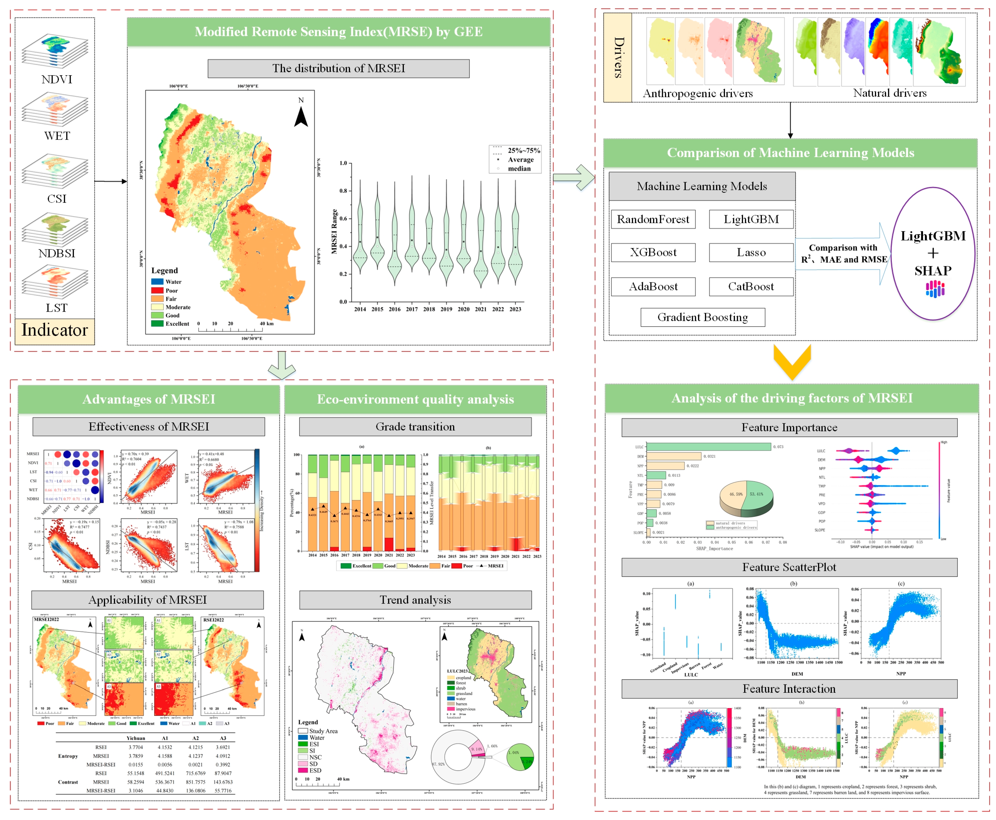
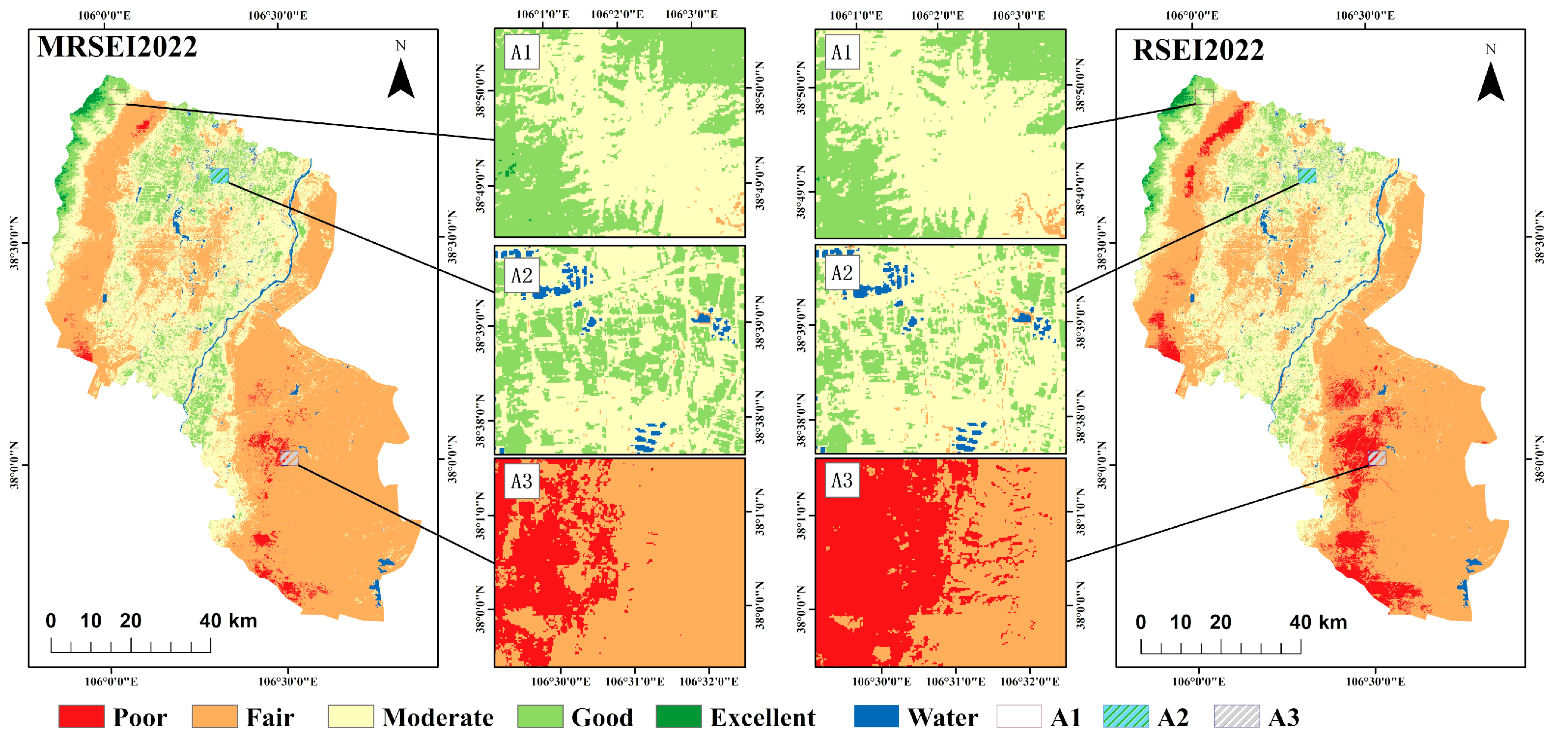
This study innovatively incorporated a salinity index (CSI) into the RSEI to construct the MRSEI. Its effectiveness for ecological assessment in arid and semi-arid regions was validated through PCA, correlation analysis, spatial comparisons, and contrast/entropy metrics. The MRSEI preserved the multi-index integration advantage of the RSEI (with a mean PC1 contribution of 79.96%) while achieving superior characterization of surface detail. Furthermore, GLCM texture analysis further confirmed the MRSEI’s enhanced performance in both entropy and contrast metrics, indicating stronger spatial heterogeneity representation capabilities.

(2)

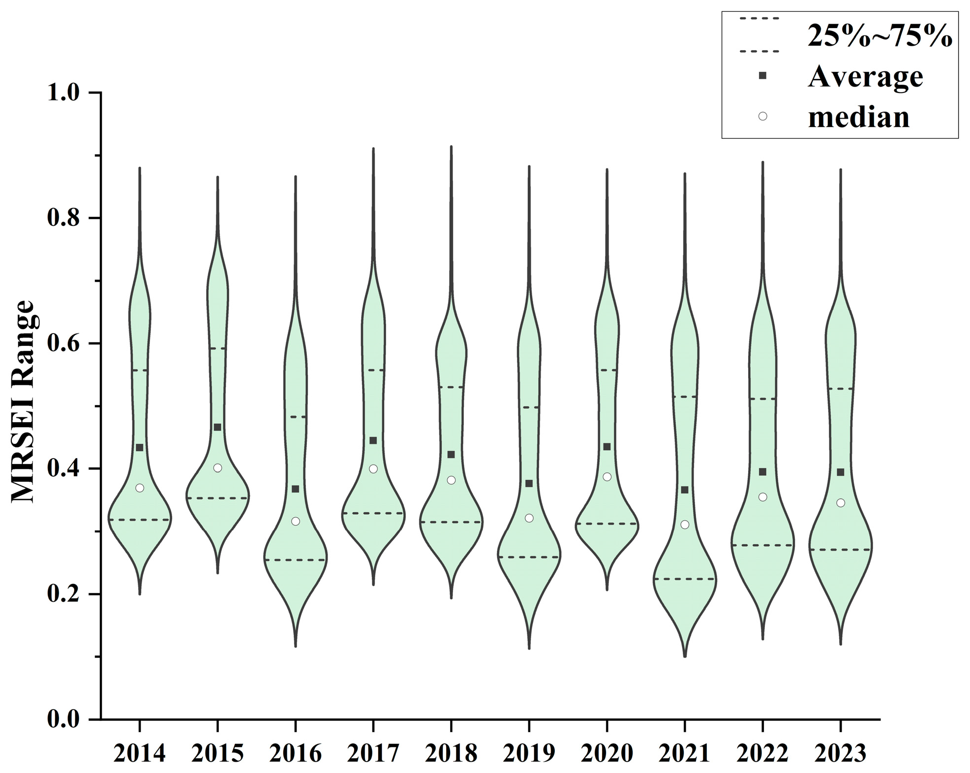
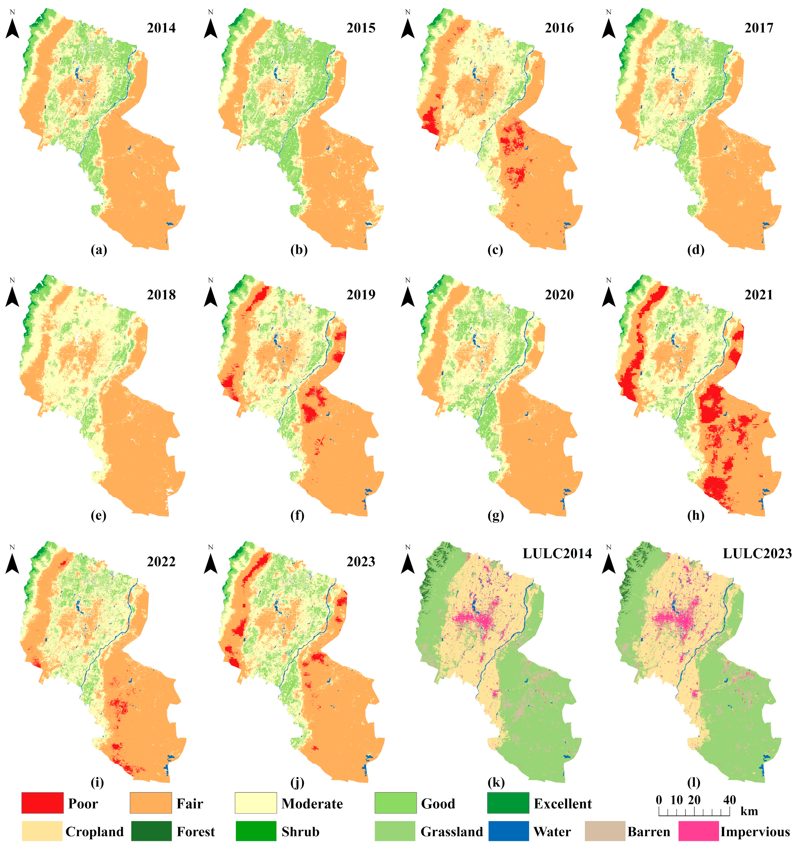
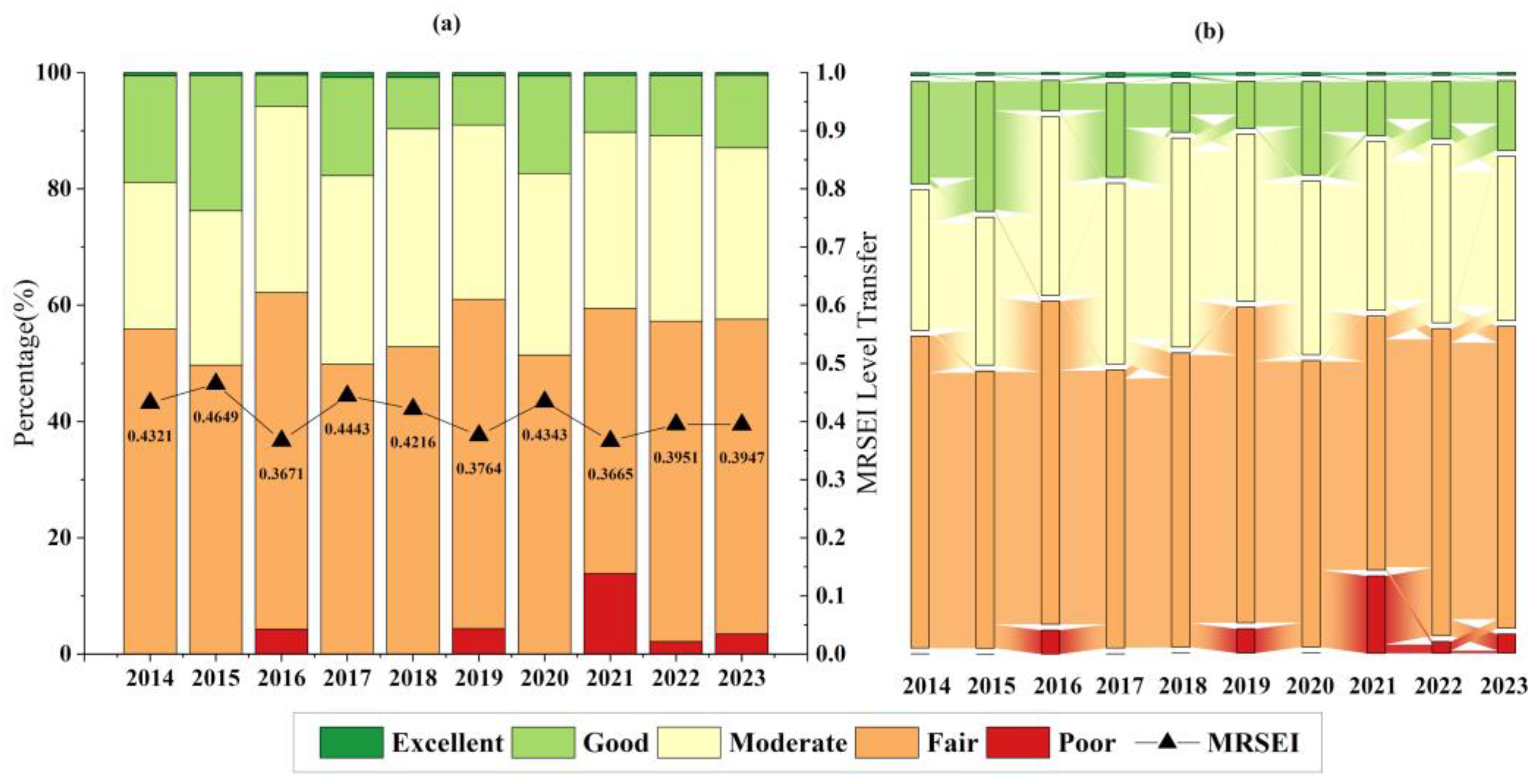
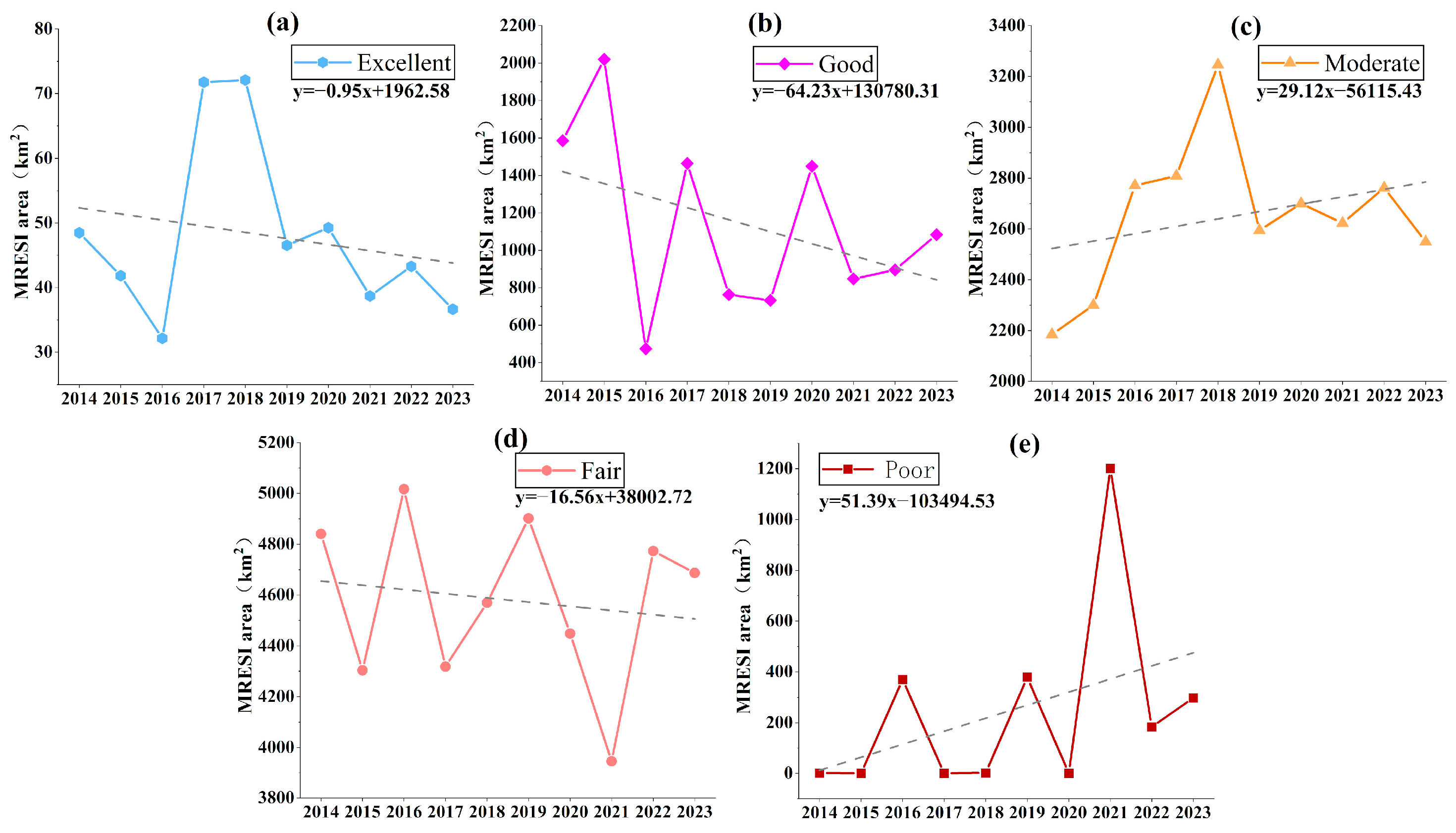
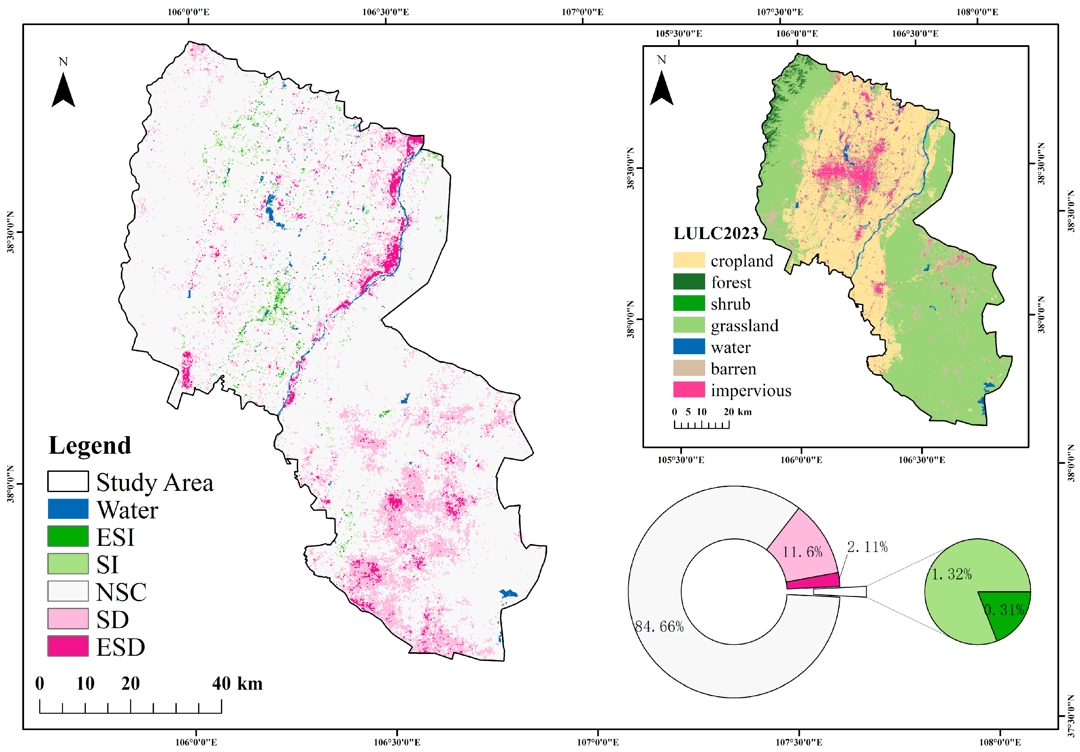
The MRSEI-based assessment of Yinchuan City’s ecological quality from 2014 to 2023 revealed a distinct spatial pattern of “higher in the northwest and lower in the southeast”. High-quality zones were primarily distributed in the western Helan Mountains and the integrated urban/rural development demonstration zone, while comparatively poorer ecological conditions were observed in the core functional zone of the provincial capital, the Helan Mountains ecological corridor, and the eastern eco-economic pilot zone. During 2014–2023, ecological quality grades were predominantly “Fair” and “Moderate”, exhibiting a distinct “W”-shaped temporal fluctuation pattern.

(3)

Trend analysis using the T–S estimator and M–K test indicated that “No Significant Change” dominated ecological trends in Yinchuan during 2014–2023, accounting for 7609.23 km² (87.92%) of the total area. Improved areas accounted for 1.28% of the total area, comprising “Extremely Significant Improvement” (21.1959 km², 0.24%) and “Significant Improvement” (89.8398 km², 1.04%). Degraded areas represented 10.80%, including “Extremely Significant Degradation” (143.8580 km², 1.66%) and “Significant Degradation” (790.6590 km², 9.14%). The substantial predominance of degraded areas indicated an overall ecological deterioration during 2014–2023.

(4)

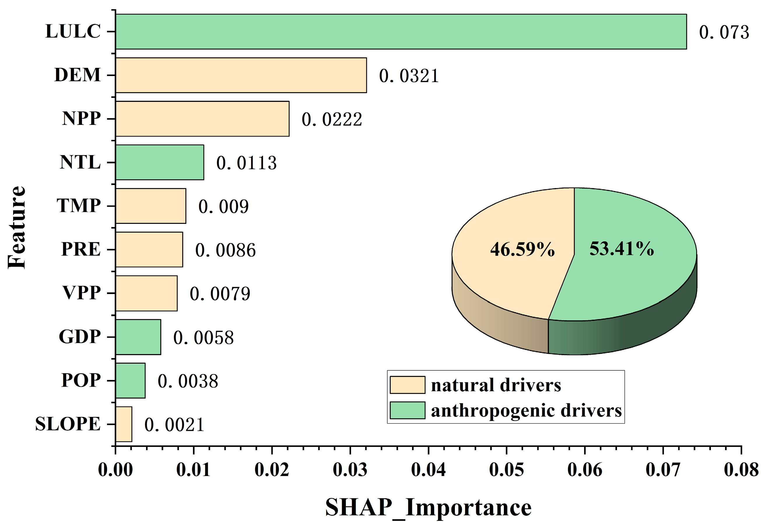
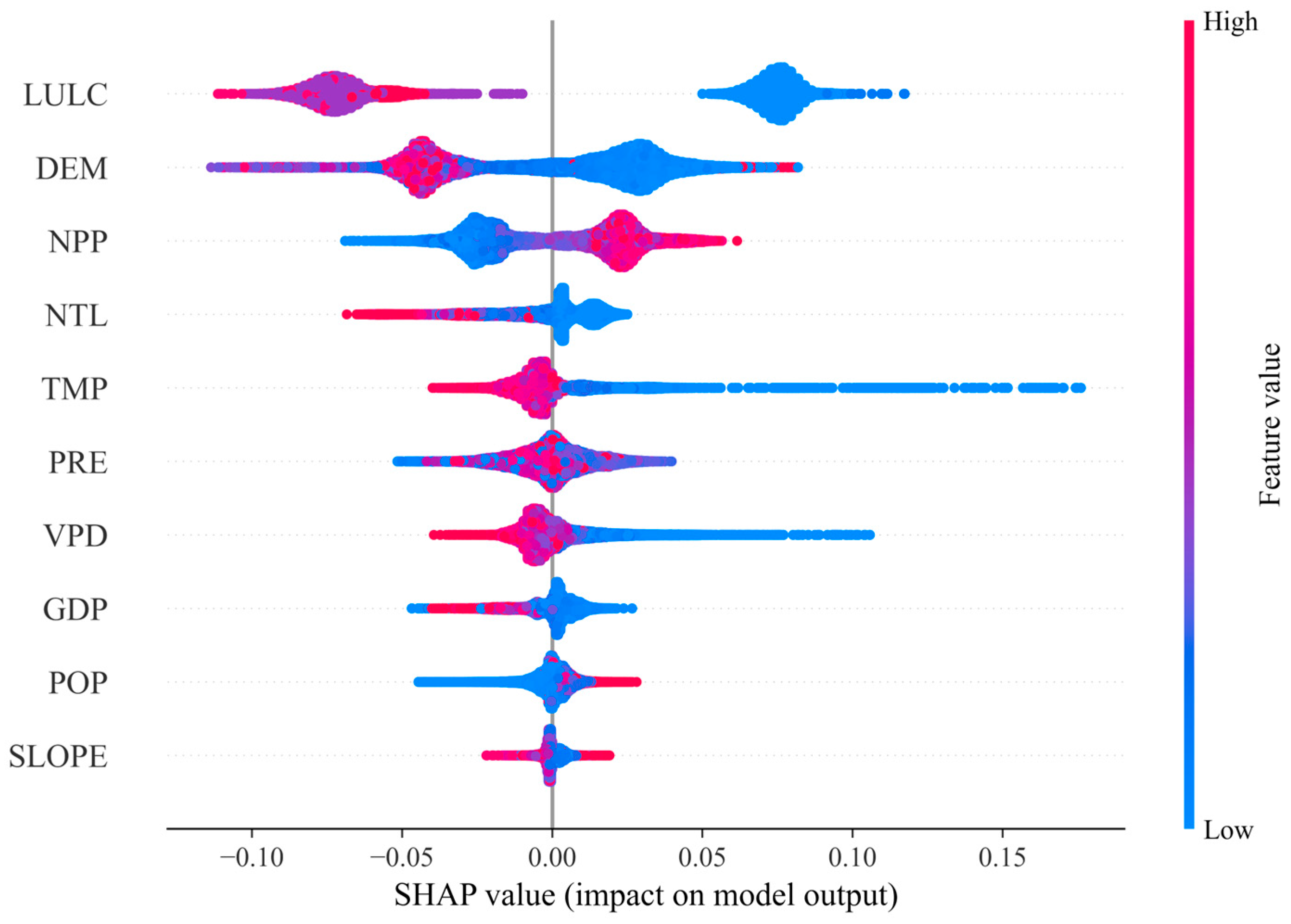
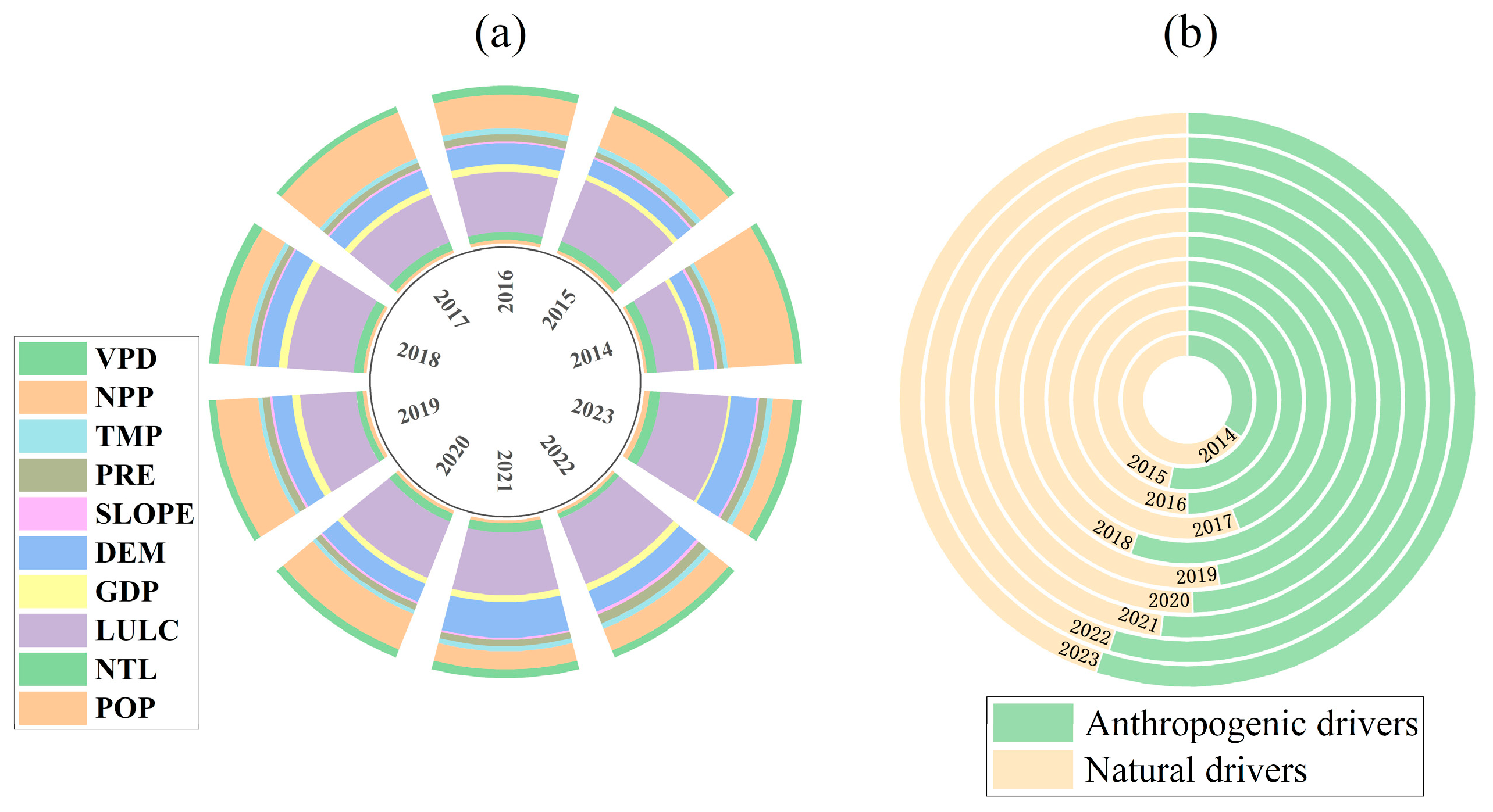
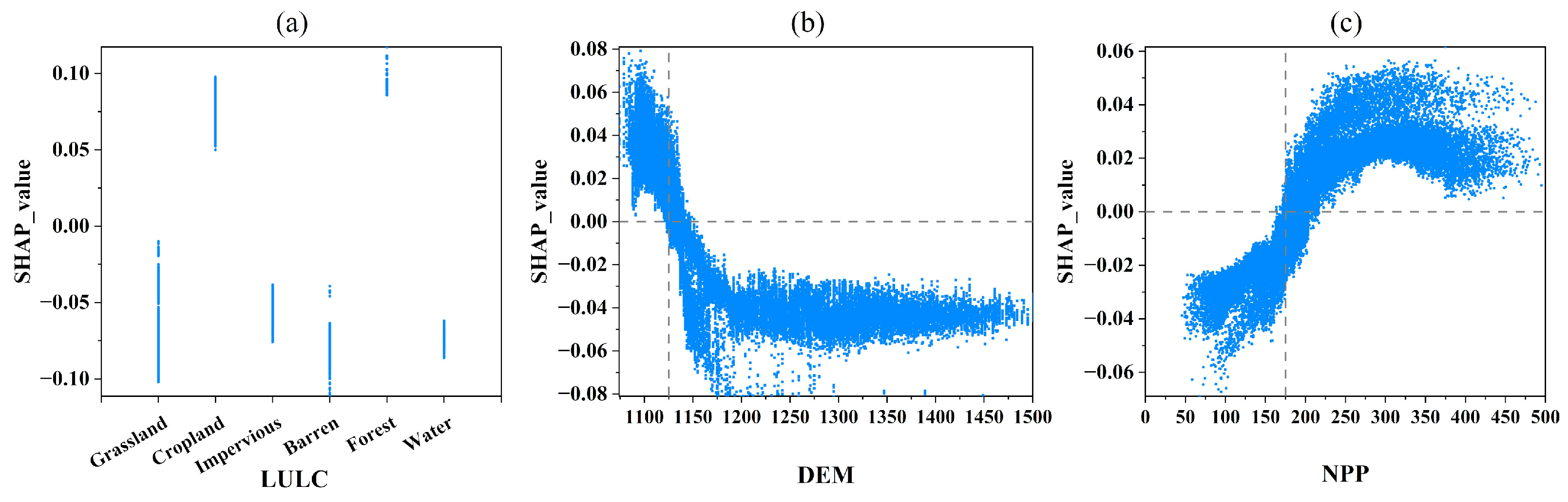
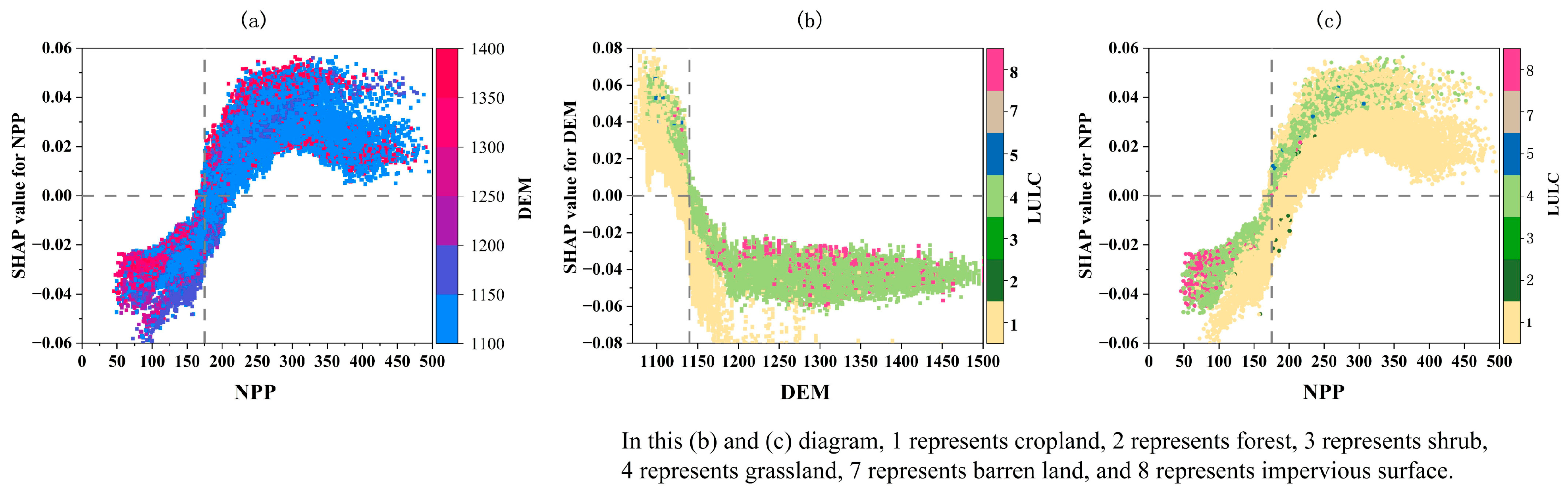
To explore ecological driving mechanisms, this study applied interpretable machine learning, combining the LightGBM model with SHAP analysis using ten representative natural and anthropogenic factors. LightGBM demonstrated optimal performance (R² = 0.6918, lowest MAE and RMSE), establishing it as the superior model. SHAP analysis identified LULC, DEM, and NPP as dominant factors: (a) cropland and forest exerted positive effects; (b) DEM (1100–1150 m) significantly enhanced the MRSEI; (c) NPP > 175 g C/m²/yr progressively improved the MRSEI. Interaction effects revealed the highest MRSEI values when NPP > 175 g C/m²/yr and DEM < 1140 m.

References

1. Yu, S.; Zhang, X.; Wang, Y.; Shen, Y. Review of research on the impacts of climate change on staple grain crops in the three provinces of Northeast China. Chin. J. Eco-Agric. 2024, 32, 970–985. [Google Scholar]
2. Jiang, Z.; Yang, Z.; Yang, Q.; Zuo, H.; Wang, Z.; Wang, J.; Tian, L. Analysis on Dynamic Change of Desertification in Kubuqi Desert During 2000–2023 Based on Landsat 8. Bull. Soil Water Conserv. 2024, 44, 118–128. [Google Scholar]
3. Han, S.; Wang, Q. Response of boreal forest ecosystem to global climate change: A review. J. Beijing For. Univ. 2016, 38, 1–20. [Google Scholar]
4. Zhang, W.; Du, P.; Guo, S.; Lin, C.; Zheng, H.; Fu, P. Enhanced remote sensing ecological index and ecological environment evaluation in arid area. Natl. Remote Sens. Bull. 2023, 27, 299–317. [Google Scholar] [CrossRef]
5. Xu, Y.; Zhou, H. A Preliminary Study on Advances in Assessment of Eco-environmenttal Quality in China. Arid Land Geogr. 2003, 26, 166–172. [Google Scholar]
6. Lingtong, D.U. Heat island effect study of Yinchuan based on landsat ETM + Data. Sci. Surv. Mapp. 2008, 33, 169–171. [Google Scholar]
7. Yuan, J.; Zhao, H.; Liu, X.; Li, H.; Jiang, D.; Zhao, C.; Xing, L.; Luo, X.; Wang, R.; Wang, C. Driving force analysis and ecological assessment of spatiotemporal changes in vegetation cover in the Kunlun Mountains from 2000 to 2020. Geol. China 2024, 51, 1822–1838. [Google Scholar]
8. Fang, C.; Zhou, C.; Gu, C.; Chen, L.; Li, S. Theoretical analysis of interactive coupled effects between urbanization and eco-environment in mega-urban agglomerations. Acta Geogr. Sin. 2016, 71, 531–550. [Google Scholar] [CrossRef]
9. Xu, H. A remote sensing urban ecological index and its application. Acta Ecol. Sin. 2013, 33, 7853–7862. [Google Scholar]
10. Yue, H.; Liu, Y.; Li, Y.; Lu, Y. Eco-Environmental Quality Assessment in China’s 35 Major Cities Based On Remote Sensing Ecological Index. IEEE Access 2019, 7, 51295–51311. [Google Scholar] [CrossRef]
11. Xiong, Y.; Xu, W.H.; Lu, N.; Huang, S.D.; Wu, C.; Wang, L.G.; Dai, F.; Kou, W.L. Assessment of spatial—Temporal changes of ecological environment quality based on RSEI and GEE: A case study in Erhai Lake Basin, Yunnan province, China. Ecol. Indic. 2021, 125, 107518. [Google Scholar] [CrossRef]
12. Sun, C.; Li, J.L.; Liu, Y.C.; Cao, L.D.; Zheng, J.H.; Yang, Z.J.; Ye, J.W.; Li, Y. Ecological quality assessment and monitoring using a time-series remote sensing-based ecological index (ts-RSEI). Gisci. Remote Sens. 2022, 59, 1793–1816. [Google Scholar] [CrossRef]
13. Liu, J.; Zhang, L.; Dong, T.; Wang, J.L.; Fan, Y.M.; Wu, H.Q.; Geng, Q.L.; Yang, Q.J.; Zhang, Z.B. The Applicability of Remote Sensing Models of Soil Salinization Based on Feature Space. Sustainability 2021, 13, 13711. [Google Scholar] [CrossRef]
14. Wang, J.; Ma, J.-L.; Xie, F.-F.; Xu, X.-J. Improvement of remote sensing ecological index in arid regions: Taking Ulan Buh Desert as an example. Ying Yong Sheng Tai Xue Bao = J. Appl. Ecol. 2020, 31, 3795–3804. [Google Scholar] [CrossRef]
15. Wang, Y.; Liu, P.; Liu, J.; Zhang, D.; Wang, L.; Huang, L. Analysis of Spatiotemporal Changes in Ecological Environment Quality of the Yellow River Delta Based on Modified Remote Sensing Ecological Index. J. Ecol. Rural Environ. 2024, 40, 1179–1190. [Google Scholar]
16. Deng, W.; Wen, X.; Xu, H.; Duan, W.; Li, C. Analysis of regional development and its ecological effects:A case study of the Xiong’an New Area, China. Acta Ecol. Sin. 2023, 43, 263–273. [Google Scholar]
17. Ariyasu, E.; Kakuta, S. Estimating Soil Salinity Using HISUI Hyperspectral Data in the Western Australian Wheatbelt. ISPRS Ann. Photogramm. Remote Sens. Spat. Inf. Sci. 2024, 10, 21–27. [Google Scholar] [CrossRef]
18. Wang, N.; Peng, J.; Chen, S.C.; Huang, J.Y.; Li, H.Y.; Biswas, A.; He, Y.; Shi, Z. Improving remote sensing of salinity on topsoil with crop residues using novel indices of optical and microwave bands. Geoderma 2022, 422, 115935. [Google Scholar] [CrossRef]
19. Allbed, A.; Kumar, L.; Aldakheel, Y.Y. Assessing soil salinity using soil salinity and vegetation indices derived from IKONOS high-spatial resolution imageries: Applications in a date palm dominated region. Geoderma 2014, 230–231, 1–8. [Google Scholar] [CrossRef]
20. Yang, S.; Han, H. Quantitative analysis of NDVI driving factors in Gansu Province based on geodetector. J. Gansu Agric. Univ. 2019, 54, 115–123. [Google Scholar]
21. Nie, T.; Dong, G.; Jiang, X.; Lei, Y.; Gao, S.; He, J. Temporal and spatial variations and driving force analysis of NDVI in Henan Province based on Geodetector. Chin. J. Ecol. 2024, 43, 273–281. [Google Scholar]
22. Zhang, R.; Li, C.; Yao, S.; Li, W. Study on the change factors of construction land in Taiyuan by integrating geographic detector and geographically weighted regression. Bull. Surv. Mapp. 2022, 106–109, 119. [Google Scholar]
23. Renyang, Q.; Lian, Y.; Li, H.; Gao, H.; Dong, J.; He, M. Spatial and temporal distribution of CO2 concentration in mainland China and its influencing factors. China Environ. Sci. 2023, 43, 1919–1929. [Google Scholar]
24. Zhang, S.; Nie, Y.; Zhang, H.; Li, Y.; Han, Y.; Liu, X.; Wang, B. Spatiotemporal Variation of Vegetation NDVI and its Driving Forces in Inner Mongolia Based on Geodetector. Acta Agrestia Sin. 2020, 28, 1460–1472. [Google Scholar]
25. Shi, Z.; Xie, H.; Wang, Z.; Hu, X.; Wang, X.; Xie, X.; Lin, H.; Liu, X. Analysis of spatiotemporal heterogeneity of habitat quality and their driving factors based on optimal parameters-based geographic detector for Fuzhou City, China. J. Environ. Eng. Technol. 2023, 13, 1921–1930. [Google Scholar]
26. Tayier, K.; Li, H.; Aierken, G.; Yin, Z.; Wu, H. Spatio-temporal Evolution and Prediction of Carbon Emissions in Urumqi Region Based on FLUS and Grey Prediction Model. J. Soil Water Conserv. 2023, 37, 214–226. [Google Scholar]
27. Zhang, L.Y.; Li, X.; Liu, X.H.; Lian, Z.Y.; Zhang, G.Z.; Liu, Z.Y.; An, S.X.; Ren, Y.X.; Li, Y.L.; Liu, S.D. Dynamic monitoring and drivers of ecological environmental quality in the Three-North region, China: Insights based on remote sensing ecological index. Ecol. Inform. 2025, 85, 102936. [Google Scholar] [CrossRef]
28. Chen, L.F.; Zhang, H.; Zhang, X.Y.; Liu, P.H.; Zhang, W.C.; Ma, X.Y. Vegetation changes in coal mining areas: Naturally or anthropogenically Driven? Catena 2022, 208, 105712. [Google Scholar] [CrossRef]
29. Sun, Z.; Xie, S. Spatiotemporal variation in net primary productivity and factor detection in Yunnan Province based on geodetector. Chin. J. Ecol. 2021, 40, 3836–3848. [Google Scholar]
30. Huang, X.; Peng, S.-Y.; Wang, Z.; Huang, B.-M.; Liu, J. Spatial heterogeneity and driving factors of ecosystem water yield service in Yunnan Province, China based on Geodetector. Ying Yong Sheng Tai Xue Bao = J. Appl. Ecol. 2022, 33, 2813–2821. [Google Scholar] [CrossRef]
31. Mu, F.; Huang, Q.; Chen, L. Eco-environmental Quality Driving Force Detection Using Optimized Geographic Detector. Res. Soil Water Conserv. 2024, 31, 440–449. [Google Scholar]
32. Asri, A.K.; Lee, H.Y.; Chen, Y.L.; Wong, P.Y.; Hsu, C.Y.; Chen, P.C.; Lung, S.C.C.; Chen, Y.C.; Wu, C.D. A machine learning-based ensemble model for estimating diurnal variations of nitrogen oxide concentrations in Taiwan. Sci. Total Environ. 2024, 916, 170209. [Google Scholar] [CrossRef] [PubMed]
33. Pelegrina, G.D.; Duarte, L.T.; Grabisch, M. A k-additive Choquet integral-based approach to approximate the SHAP values for local interpretability in machine learning. Artif. Intell. 2023, 325, 104014. [Google Scholar] [CrossRef]
34. Li, Z.Q. Extracting spatial effects from machine learning model using local interpretation method: An example of SHAP and XGBoost. Comput. Environ. Urban Syst. 2022, 96, 101845. [Google Scholar] [CrossRef]
35. Khan, N.M.; Rastoskuev, V.V.; Sato, Y.; Shiozawa, S. Assessment of hydrosaline land degradation by using a simple approach of remote sensing indicators. Agric. Water Manag. 2005, 77, 96–109. [Google Scholar] [CrossRef]
36. Xiaolei, L.I.U.; Zhihao, Q.I.N. Comparative Analysis between NDWI and NDVI Indices in Regional Drought Monitoring. Remote Sens. Technol. Appl. 2007, 22, 608–612. [Google Scholar]
37. Lobser, S.E.; Cohen, W.B. MODIS tasselled cap: Land cover characteristics expressed through transformed MODIS data. Int. J. Remote Sens. 2007, 28, 5079–5101. [Google Scholar] [CrossRef]
38. Xu, H. A new index for delineating built-up land features in satellite imagery. Int. J. Remote Sens. 2008, 29, 4269–4276. [Google Scholar] [CrossRef]
39. Liu, Y.X.; Wang, Y.L.; Peng, J.; Du, Y.Y.; Liu, X.F.; Li, S.S.; Zhang, D.H. Correlations between Urbanization and Vegetation Degradation across the World’s Metropolises Using DMSP/OLS Nighttime Light Data. Remote Sens. 2015, 7, 2067–2088. [Google Scholar] [CrossRef]
40. Li, Y.M.; Li, Y.T.; Yang, X.; Feng, X.J.; Lv, S.B. Evaluation and driving force analysis of ecological quality in Central Yunnan Urban Agglomeration. Ecol. Indic. 2024, 158, 111598. [Google Scholar] [CrossRef]
41. Amirataee, B.; Montaseri, M. The performance of SPI and PNPI in analyzing the spatial and temporal trend of dry and wet periods over Iran. Nat. Hazards 2017, 86, 89–106. [Google Scholar] [CrossRef]
42. Chen, C.; Wang, L.Y.; Yang, G.; Sun, W.W.; Song, Y.Z. Mapping of Ecological Environment Based on Google Earth Engine Cloud Computing Platform and Landsat Long-Term Data: A Case Study of the Zhoushan Archipelago. Remote Sens. 2023, 15, 4072. [Google Scholar] [CrossRef]
43. Garzón, M.B.; Blazek, R.; Neteler, M.; de Dios, R.S.; Ollero, H.S.; Furlanello, C. Predicting habitat suitability with machine learning models: The potential area of Pinus sylvestris L. in the Iberian Peninsula. Ecol. Model. 2006, 197, 383–393. [Google Scholar] [CrossRef]
44. Chen, Y.; Zhao, Q.; Liu, Y.M.; Zeng, H. Exploring the impact of natural and human activities on vegetation changes: An integrated analysis framework based on trend analysis and machine learning. J. Environ. Manag. 2025, 374, 124092. [Google Scholar] [CrossRef]
45. Ueda, K.; Suwa, H.; Yamada, M.; Ogawa, Y.; Umehara, E.; Yamashita, T.; Tsubouchi, K.; Yasumoto, K. SSCDV: Social media document embedding with sentiment and topics for financial market forecasting. Expert Syst. Appl. 2024, 245, 122988. [Google Scholar] [CrossRef]
46. Segal, M.; Xiao, Y.Y. Multivariate random forests. Wiley Interdiscip. Rev. Data Min. Knowl. Discov. 2011, 1, 80–87. [Google Scholar] [CrossRef]
47. Tian, S.; Guo, H.W.; Xu, W.; Zhu, X.T.; Wang, B.; Zeng, Q.H.; Mai, Y.Q.; Huang, J.H.J. Remote sensing retrieval of inland water quality parameters using Sentinel-2 and multiple machine learning algorithms. Environ. Sci. Pollut. Res. 2023, 30, 18617–18630. [Google Scholar] [CrossRef]
48. Chen, J.J.; Du, H.Q.; Mao, F.J.; Huang, Z.H.; Chen, C.; Hu, M.C.; Li, X.J. Improving forest age prediction performance using ensemble learning algorithms base on satellite remote sensing data. Ecol. Indic. 2024, 166, 112327. [Google Scholar] [CrossRef]
49. Wang, C.; Sheng, Q.Q.; Zhu, Z.L. Exploring Ecological Quality and Its Driving Factors in Diqing Prefecture, China, Based on Annual Remote Sensing Ecological Index and Multi-Source Data. Land 2024, 13, 1499. [Google Scholar] [CrossRef]
50. Yang, Y.Z.; Meng, Z.J.; Zu, J.X.; Cai, W.H.; Wang, J.L.; Su, H.X.; Yang, J. Fine-Scale Mangrove Species Classification Based on UAV Multispectral and Hyperspectral Remote Sensing Using Machine Learning. Remote Sens. 2024, 16, 3093. [Google Scholar] [CrossRef]
51. Tibshirani, R. Regression shrinkage and selection via the lasso: A retrospective. J. R. Stat. Soc. Ser. B-Stat. Methodol. 2011, 73, 273–282. [Google Scholar] [CrossRef]
52. Qi, T.J.; Zhao, Y.; Meng, X.M.; Shi, W.; Qing, F.; Chen, G.; Zhang, Y.; Yue, D.X.; Guo, F.Y. Distribution Modeling and Factor Correlation Analysis of Landslides in the Large Fault Zone of the Western Qinling Mountains: A Machine Learning Algorithm. Remote Sens. 2021, 13, 4990. [Google Scholar] [CrossRef]
53. Chen, H.; Covert, I.C.; Lundberg, S.M.; Lee, S.I. Algorithms to estimate Shapley value feature attributions. Nat. Mach. Intell. 2023, 5, 590–601. [Google Scholar] [CrossRef]
54. Lundberg, S.M.; Erion, G.; Chen, H.; DeGrave, A.; Prutkin, J.M.; Nair, B.; Katz, R.; Himmelfarb, J.; Bansal, N.; Lee, S.I. From local explanations to global understanding with explainable AI for trees. Nat. Mach. Intell. 2020, 2, 56–67. [Google Scholar] [CrossRef]
55. Xu, H.; Deng, W. Rationality Analysis of MRSEI and Its Difference with RSEI. Remote Sens. Technol. Appl. 2022, 37, 1–7. [Google Scholar]
56. Wang, J.; He, J.; Qu, G.; Hou, J.; Wang, H. Temporal and spatial evolution of eco-environmental quality and its driving factors in Yinchuan city. Southwest China J. Agric. Sci. 2023, 36, 2780–2792. [Google Scholar]
57. Zhang, X.; Chen, L.; Ma, Y.; Huang, Z.; Li, Y. Monitoring and evaluation of ecology and environment quality of Yinchuan City based on GIS and RS. J. Saf. Environ. 2021, 21, 2854–2864. [Google Scholar]
58. Wang, B.; Yang, T.B. Assessing Impact of Land Use Change on the Ecosystem Service Value in Yinchuan City from 1980 to 2018. Sustainability 2021, 13, 8311. [Google Scholar] [CrossRef]
59. Ma, Y.X.; Tashpolat, N. Remote Sensing Monitoring of Soil Salinity in Weigan River-Kuqa River Delta Oasis Based on Two-Dimensional Feature Space. Water 2023, 15, 1694. [Google Scholar] [CrossRef]
60. Wu, X.; Wang, Z.; Fan, L.; Li, L. An applicability analysis of salinization evaluation index based on multispectral remote sensing to soil salinity prediction in Yinbei irrigation area of Ningxia. Remote Sens. Land Resour. 2021, 33, 124–133. [Google Scholar]
61. Cao, L.; Ding, J.; Umut, H.; Su, W.; Ning, J.; Miao, C.; Li, H. Extraction and Modeling of Regional Soil Salinization Based on Data from GF-1 Satellite. Acta Pedol. Sin. 2016, 53, 1399–1409. [Google Scholar]
62. Zhang, H.; Wang, W.; Song, Y.; Miao, L.; Ma, C. Ecological index evaluation of arid inflow area based on the modified remote sensing ecological index:a case study of Tabu River Basin at the northern foot of the Yin Mountains. Acta Ecol. Sin. 2024, 44, 523–543. [Google Scholar]
63. Wu, D.; Jia, K.L.; Zhang, X.D.; Zhang, J.H.; Abd El-Hamid, H.T. Remote Sensing Inversion for Simulation of Soil Salinization Based on Hyperspectral Data and Ground Analysis in Yinchuan, China. Nat. Resour. Res. 2021, 30, 4641–4656. [Google Scholar] [CrossRef]
64. Peng, J.; Liu, H.; Shi, Z.; Xiang, H.; Chi, C. Regional heterogeneity of hyperspectral characteristics of salt-affected soil and salinity inversion. Trans. Chin. Soc. Agric. Eng. 2014, 30, 167–174. [Google Scholar]
65. Bai, Z.F.; Han, L.; Liu, H.Q.; Jiang, X.H.; Li, L.Z. Spatiotemporal change and driving factors of ecological status in Inner Mongolia based on the modified remote sensing ecological index. Environ. Sci. Pollut. Res. 2023, 30, 52593–52608. [Google Scholar] [CrossRef]
66. Zhang, X.X.; Wang, X.X.; Li, W.P.; Wu, X.D.; Cheng, X.Q.; Zhou, Z.Y.; Ling, Q.; Liu, Y.D.; Liu, X.J.; Hao, J.M.; et al. Dynamic Monitoring and Analysis of Ecological Environment Quality in Arid and Semi-Arid Areas Based on a Modified Remote Sensing Ecological Index (MRSEI): A Case Study of the Qilian Mountain National Nature Reserve. Remote Sens. 2024, 16, 3530. [Google Scholar] [CrossRef]
67. Feng, Z.; She, L.; Wang, X.; Yang, L.; Yang, C. Spatial and Temporal Variations of Ecological Environment Quality in Ningxia Based on Improved Remote Sensing Ecological Index. Ecol. Environ. Sci. 2024, 33, 131–143. [Google Scholar]
68. Liu, Y.-W.; Liu, C.-W.; He, Z.-Y.; Zhou, X.; Han, B.-H.; Hao, H.-Z. Spatial-temporal evolution of ecological land and influence factors in Wuhan urban agglome-ration based on geographically weighted regression model. Ying Yong Sheng Tai Xue Bao = J. Appl. Ecol. 2020, 31, 987–998. [Google Scholar] [CrossRef]
69. Guo, S.; Yang, W.; Wei, M.; Yang, Y.; Zhang, P. Cultivated Land Fragmentation and Impact Factors of Qinglong Manchu Autonomous County Based on Geographically Weighted Regression. Res. Soil Water Conserv. 2017, 24, 264–269. [Google Scholar]
70. Sun, L.; Zhou, D.; Cen, G.; Ma, J.; Dang, R.; Ni, F.; Zhang, J. Landscape ecological risk assessment and driving factors of the Shule River Basin based on the geographic detector model. Arid Land Geogr. 2021, 44, 1384–1395. [Google Scholar]
71. Fan, S.; Liu, Z.; Zhu, M.; Zhang, M. Time series change and influencing factors of land use in Guangzhou city based on geodetector. Southwest China J. Agric. Sci. 2022, 35, 2276–2289. [Google Scholar]
72. Guo, J.P.; Shen, B.B.; Li, H.X.; Wang, Y.D.; Tuvshintogtokh, I.; Niu, J.M.; Potter, M.A.; Yonghong, F. Past dynamics and future prediction of the impacts of land use cover change and climate change on landscape ecological risk across the Mongolian plateau. J. Environ. Manag. 2024, 355, 120365. [Google Scholar] [CrossRef] [PubMed]
73. Xie, B.Q.; Ding, J.L.; Ge, X.Y.; Li, X.H.; Han, L.J.; Wang, Z. Estimation of Soil Organic Carbon Content in the Ebinur Lake Wetland, Xinjiang, China, Based on Multisource Remote Sensing Data and Ensemble Learning Algorithms. Sensors 2022, 22, 2685. [Google Scholar] [CrossRef] [PubMed]
74. Chen, W.; Wang, J.J.; Ding, J.L.; Ge, X.Y.; Han, L.J.; Qin, S.F. Detecting Long-Term Series Eco-Environmental Quality Changes and Driving Factors Using the Remote Sensing Ecological Index with Salinity Adaptability (RSEISI): A Case Study in the Tarim River Basin, China. Land 2023, 12, 1309. [Google Scholar] [CrossRef]
75. Li, Z.M.; Man, W.; Peng, J.H.; Wang, Y.; Nie, Q.; Sun, F.Q.; Huang, Y.T. Spatiotemporal Variation in Ecological Environmental Quality and Its Response to Different Factors in the Xia-Zhang-Quan Urban Agglomeration over the Past 30 Years. Land 2024, 13, 1078. [Google Scholar] [CrossRef]
Figure 1. Location of Yinchuan City. (a) Location of NINGXIA HUIZU ZIZHIQU in China. (b) Location of Yinchuan City in NINGXIA HUIZU ZIZHIQU. (c) Yinchuan City territorial spatial zoning and topographic map.
Remotesensing 17 02266 g001
Figure 2. Workflow of the study.
Remotesensing 17 02266 g002
Figure 3. The correlations between individual indicators and the MRSEI.
Remotesensing 17 02266 g003
Figure 4. The selection of typical regions. (A1A3) denote the selected representative regions.
Remotesensing 17 02266 g004
Figure 5. Comparison between the MRSEI and RSEI in typical regions. (A1A3) denote the selected representative regions.
Remotesensing 17 02266 g005
Figure 6. Statistical results of the MRSEI for Yinchuan City (2014–2023).
Remotesensing 17 02266 g006
Figure 7. (aj) MRSEI distribution maps of Yinchuan City from 2014 to 2023, respectively. (k,l) LULC maps for the years 2014 and 2023, respectively.
Remotesensing 17 02266 g007
Figure 8. MRSEI grade distribution statistics and grade transition Sankey diagrams. (a) Bar plots of MRSEI grade percentages and line plots of MRSEI mean values. (b) MRSEI grade transitions during the study period.
Remotesensing 17 02266 g008
Figure 9. Annual MRSEI grade variation trends. (ae) indicate the yearly trends of MRSEI grades, namely Excellent, Good, Moderate, Fair, and Poor, respectively. The gray dashed lines represent linear fitting lines, illustrating the trend over time for each MRSEI grade.
Remotesensing 17 02266 g009
Figure 10. The spatial distribution of MRSEI trends.
Remotesensing 17 02266 g010
Figure 11. Importance ranking according to |SHAP value|.
Remotesensing 17 02266 g011
Figure 12. SHAP summary plot.
Remotesensing 17 02266 g012
Figure 13. Annual statistics of driving factors (2014–2023). (a) Annual contribution rates of driving factors. (b) Annual contribution rates of natural and anthropogenic factors.
Remotesensing 17 02266 g013
Figure 14. SHAP dependency plot for LightGBM. (a) Scatter plot of SHAP values for LULC. (b) Scatter plot of SHAP values for DEM. (c) Scatter plot of SHAP values for NPP.
Remotesensing 17 02266 g014
Figure 15. Interaction effects of multiple drivers. (a) Interaction effects between NPP and DEM in LightGBM. (b) Interaction effects between DEM and LULC in LightGBM. (c) Interaction effects between NPP and LULC in LightGBM.
Remotesensing 17 02266 g015