Abstract
While deep learning has advanced object detection through hierarchical feature learning and end-to-end optimization, conventional random sampling paradigms exhibit critical limitations in addressing hyperspectral ambiguity and low-distinguishability challenges in ground-based cloud detection. To overcome these limitations, we propose CurriCloud, a loss-adaptive curriculum framework featuring three key innovations: (1) real-time sample evaluation via Unified Batch Loss (UBL) for difficulty measurement, (2) stabilized training monitoring through a sliding window queue mechanism, and (3) progressive sample selection aligned with model capability using meteorology-guided phase-wise threshold scheduling. Extensive experiments on the ALPACLOUD benchmark demonstrate CurriCloud’s effectiveness across diverse architectures (YOLOv10s, SSD, and RT-DETR-R50), achieving consistent improvements of +3.1% to +11.4% mAP50 over both random sampling baselines and existing curriculum learning methods.
1. Introduction
Ground-based cloud detection, as a core component of meteorological observation systems, plays a crucial role in analyzing weather transitions and multi-domain meteorological services [1,2,3].
Different cloud types indicate distinct weather patterns. For instance, mammatus clouds are often associated with hail or extreme weather events, while altocumulus lenticularis clouds signal strong wind shear and high aviation turbulence risk. Consequently, real-time, high-precision ground-based cloud detection is essential for localized short-term extreme weather warnings. This capability also proves vital for photovoltaic power generation forecasting [4], as cloud movement and morphological changes directly influence solar radiation distribution, thereby affecting photovoltaic plant efficiency. Ground-based cloud monitoring systems capture precise spatiotemporal cloud characteristics, enabling optimization of power prediction models and reduced output intermittency. As a specialized form of remote sensing imagery, ground-based cloud observations provide higher-resolution data than satellite counterparts [5], compensating for spatiotemporal detail limitations in satellite observations while enhancing meteorological research and applications.
However, ground-based cloud detection faces numerous technical challenges. First, cloud morphology exhibits high diversity and complexity [6], as illustrated in Figure 1 [5]. Different cloud categories may share similar visual features. For example, opaque altostratus and nimbostratus clouds are often indistinguishable to untrained observers. Second, ground-based clouds and certain surface features (e.g., deserts, snow-covered terrain) exhibit spectral similarities, increasing the risk of false detection. Furthermore, the non-rigid atmospheric phenomena of ground-based clouds and the presence of occlusion effects leads to boundary ambiguity, significantly complicating detection.
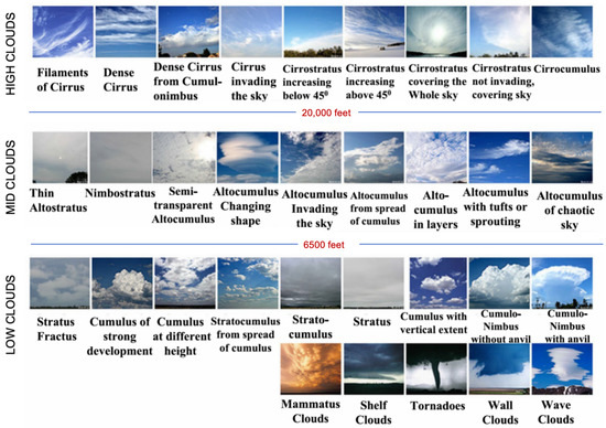
Figure 1.
Different cloud categories [5]. Cloud morphology exhibits high diversity and complexity.
These challenges limit the effectiveness of traditional machine learning methods based on handcrafted features [7,8,9]. In recent years, deep learning techniques—particularly CNNs and Transformers—have achieved remarkable progress in remote sensing image analysis, including key tasks such as object localization and recognition [10,11,12,13,14,15]. However, directly applying generic detection models (e.g., RS-Mamba [12], DBSANet [13], SAIP-Net [14], YOLO series [10,16,17], and RT-DETR [11,18]) to ground-based cloud detection yields limited performance due to training domain bias and the unique physical properties of ground-based clouds. While some studies attempt performance improvements through model refinement [15,19,20] or transfer learning [21,22], conventional random sampling paradigms overlook inherent sample difficulty variability and its impact on model learning. This often results in limited generalization for complex scenarios, manifesting as misclassification and false detection. Key unresolved challenges include complex cloud morphology, inter-class visual similarity, and dynamic background interference.
Curriculum learning (CL) [23], a machine learning paradigm inspired by human education, was first introduced by Bengio et al. and validated both theoretically and empirically. Its fundamental premise involves progressively training models from simple to complex samples to improve learning efficiency and final performance. CL operates on three key principles: (1) quantifiable difficulty differences among samples, where easier examples enable faster development of effective feature representations; (2) knowledge accumulation, where simple features form foundations for learning complex patterns; and (3) dynamic adaptation, where optimal learning progression adjusts based on real-time model performance to optimize neural network parameter exploration [23].
These principles naturally align with CNNs’ hierarchical feature extraction and the multidimensional challenges of cloud detection. While CL has demonstrated success across computer vision domains [24,25], its application to cloud detection remains underexplored. To address this gap, we propose CurriCloud, a loss-adaptive curriculum learning framework designed for ground-based cloud detection that dynamically adjusts sample difficulty during progressive training. The core innovations include (1) a loss-adaptive difficulty measurement evaluating sample complexity based on real-time training performance; (2) a meteorologically-guided phase-wise threshold scheduling mechanism that progressively matches sample selection to the model’s evolving capability; and (3) a loss sliding window leveraging limited memory adaptability and sample-variation tolerance to monitor training loss distribution, reducing outdated data influence while accommodating meteorological data non-stationarity.
The main contributions of this work are summarized as follows:
- We propose CurriCloud, a curriculum learning framework featuring loss-adaptive difficulty estimation and dynamic scheduling mechanisms for ground-based cloud detection. This framework utilizes Unified Batch Loss (UBL) with a loss sliding window queue for stable sample evaluation, and meteorologically guided phase-wise threshold scheduling to progressively align sample selection with model capability.
- We construct ALPACLOUD, a novel ground-based cloud image dataset containing diverse terrestrial backgrounds. Unlike existing all-sky or pure-sky cloud datasets, ALPACLOUD better reflects real-world scenarios and enhances model robustness against background interference.
- We conduct comprehensive experiments validating CurriCloud’s effectiveness across multiple detection architectures on the ALPACLOUD benchmark, demonstrating consistent performance improvements.
2. Related Works
2.1. Ground-Based Cloud Detection
Ground-based cloud detection addresses two core objectives: (1) cloud localization and (2) cloud type classification.
As a type of remote sensing imagery, ground-based cloud classification requires the fusion of both large-scale global features and fine-grained local features, with recent advances in Transformer- and CNN-based deep learning models being widely applied to this field. RS-Mamba [12] processes full-resolution images without patch segmentation, preserving contextual information through global multi-directional modeling, while DBSANet [13] overcomes convolutional limitations via a ResNet-Swin Transformer dual-branch architecture, and SAIP-Net [14] employs adaptive frequency filtering to suppress intra-class inconsistencies. Cross-domain insights emerge from TransUNet [26], whose CNN–Transformer hybrid encoder balances global–local features for medical images, and CGAT [27], which models cloud spatial relationships through graph networks with attention-based feature stabilization. However, these methods exhibit three key limitations: (1) they remain overly dependent on spatial–contextual features, making them sensitive to illumination and atmospheric changes that distort visual morphology while preserving physical cloud categories; (2) current architectures predominantly treat classification as a static task, neglecting critical temporal evolution patterns; and (3) they fail to adequately address the non-rigid, spatiotemporal nature of clouds. These challenges collectively highlight the need for ground-based cloud classification methods to integrate physics-informed feature representation and dynamic modeling capabilities.
For ground-based cloud recognition tasks involving similar-background object distinction, CM-YOLO [20] enhances feature representation through (1) synergistic integration of global contextual information extracted via hierarchical selective attention mechanisms and (2) CNN-captured local features. This approach combines optical property analysis with adaptive background subtraction to effectively suppress environmental interference while enhancing target contrast. Methodological parallels exist in AAformer [28], whose patch-level alignment scheme—originally developed for human/non-human part recognition—provides transferable insights for separating cloud structures from complex backgrounds. Current research addresses additional challenges through [29]’s multi-task learning framework for handling intra-class variability and occlusion robustness, complemented by [21,22]’s transfer learning solutions for data-scarce scenarios. Nevertheless, these approaches still exhibit accuracy gaps that require further investigation.
Operational meteorology increasingly demands precise and efficient systems capable of simultaneous localization and classification. Modern generic object detectors show particular promise: the CNN-based YOLO series [10,17] achieves real-time performance through efficient single-stage architecture, while Transformer-based DETRs [11,18] eliminate conventional components like anchor boxes and non-maximum suppression via end-to-end design.
Due to the unique characteristics of ground-based clouds, generic object detection models (e.g., YOLOs, DETRs, SSDs) exhibit significant limitations in ground-based cloud detection tasks.
Ground-based clouds display non-rigid properties (blurred boundaries, dynamic deformation), while Transformers rely on rigid grid-based feature partitioning and fixed learnable queries. This design struggles to adapt to continuous ground-based cloud deformations (e.g., cumulonimbus vertical development) or semi-transparent regions (e.g., cirrus filaments), resulting in poor bounding box fitting for ambiguous edges. Additionally, Transformers’ self-attention mechanisms may overfocus on spectrally similar backgrounds (snowfields, building reflections) due to lacking domain-specific constraints. Although DETR suppresses redundant predictions via Hungarian matching, it remains ineffective against meteorological false positives (haze vs. stratus).
CNN-based models like YOLOv10 improve gradient flow but show persistent Feature Pyramid Network (FPN) limitations when handling extreme cloud-scale variations. Significant performance gaps exist between detecting thin cirrus (large-scale, low-contrast) and broken cumulus (small-scale, high-contrast). Optimized anchor mechanisms still fail to accurately fit non-rigid cloud boundaries.
These issues are exacerbated by traditional random sampling strategies, which ignore inherent difficulty distributions. Uniform sampling causes inefficient learning on challenging samples (thin cirrus, fractured clouds) and prevents dynamic weight adjustment during training.
Curriculum learning addresses these challenges through progressive “easy-to-hard” training (e.g., distinct cumulus to broken stratocumulus) combined with difficulty-aware sampling, thereby enhancing model robustness under complex meteorological conditions.
2.2. Curriculum Learning
CL has demonstrated significant effectiveness in computer vision and object detection [23,24,25,30], providing valuable references for ground-based cloud detection.
A general CL framework comprises two core components:
(1) A difficulty measurer that determines the relative complexity of each sample, (2) A training scheduler that sequences data subsets throughout training based on difficulty assessments [23].
Curriculum Learning paradigms are categorized as static or dynamic based on sample difficulty measurement approaches. Static CL predefines sample difficulty using fixed metrics before training and maintains constant difficulty levels throughout the process [23,31,32,33]. For instance, samples containing fewer and larger objects are typically considered easier [32,33]. Alternative approaches employ difficulty estimators [31] or utilize prediction confidence levels from neural networks [34] to approximate sample complexity. Other studies [30,35] leverage errors from pre-trained models to estimate sample difficulty. The primary limitation of static CL is its inability to dynamically adjust difficulty based on learner feedback.
The dynamic CL paradigm continuously adjusts sample difficulty according to the model’s evolving learning capacity during training. Self-paced learning (SPL) [36], a classic dynamic method, ranks samples from easy to hard based on real-time learning progress. For instance, inputs with lower loss values at specific training stages are considered easier than those with higher loss. SPL has been successfully implemented in multiple solutions [34,37,38,39,40]. Self-paced curriculum learning (SPCL) [33,40,41], which integrates SPL with pre-computed difficulty metrics, incorporates both pre-training prior knowledge and real-time learning progress. Conceptually analogous to human education, SPCL represents an ’instructor–student collaborative’ mode—distinct from the instructor-driven CL approach or student-driven SPL methodology.
Current SPL solutions rely on instantaneous loss values while ignoring samples’ intrinsic difficulty, potentially causing misjudgments in cloud detection. Specifically, (a) morphologically complex stratocumulus clouds may be misclassified as “hard” due to transient localization loss spikes, even when exhibiting clearly distinguishable categorical features, while (b) fragmented clouds with significant intra-class variation are often prematurely incorporated into training owing to deceptively low loss values, causing models to overlook their inherent diversity.
Although SPCL incorporates predefined difficulty metrics (e.g., cloud layer count, target size), these indicators fail to address meteorologically critical challenges. A fundamental limitation arises when characterizing intra-class variations—such as the broken/continuous forms of stratocumulus clouds—using simplified physical attributes, as such metrics are fundamentally incapable of capturing the nuanced morphological spectrum essential for comprehensive cloud analysis.
Unlike SPL and SPCL which operate at the data level, certain dynamic CL methods function at the model level by progressively increasing neural architecture model capacity. For example, the LeRaC method [42] employs layer-specific learning rates to assign higher values to input-proximal layers, while CBS [43] applies feature smoothing in CNNs to reduce noise through progressive information integration that enhances learned feature maps. However, CBS suppresses noise via Gaussian kernel smoothing but risks losing critical high-frequency details (e.g., thin cloud edges) when excessively applied; similarly, LeRaC optimizes training through layer-wise learning rates yet lacks dynamic difficulty assessment capabilities.
Our work extends these approaches by implementing sliding-window loss distribution monitoring to achieve precise model-capability-to-sample-difficulty alignment. The innovation of CurriCloud lies in dynamically decoupling intrinsic difficulty from interference factors through real-time loss distribution analysis with meteorologically-guided phased thresholds (e.g., the 0.9 quantile threshold for thin cloud differentiation), thereby overcoming the aforementioned limitations.
2.3. Loss Functions for Object Detection
The performance of detection models hinges critically on the design of loss functions, which simultaneously optimize localization accuracy (i.e., bounding box regression) and classification confidence while balancing gradient contributions across subtasks. Modern detection losses typically integrate three kinds of key components:
- Classification Loss: This measures the discrepancy between predicted and ground-truth class labels. Widely adopted variants include Cross-Entropy (CE) loss and Focal Loss [44].
- Localization Loss: This quantifies spatial deviations between predicted and ground-truth bounding boxes. Early frameworks relied on L1/L2, or Smooth L1 norms [45], while recent advancements introduced Intersection over Union (IoU)-based losses such as GIoU [46] and GCIoU [47].
- Auxiliary Losses: Advanced frameworks incorporate domain-specific constraints. For example, YOLOv10 [17] employs Distribution Focal Loss (DFL) to model bounding box distribution statistics, enhancing robustness in detecting irregular geological features.
The loss value serves as an indicator of the model’s current detection capability for a given sample. Different detection models employ distinct loss types and loss combination strategies, reflecting specialized optimizations for specific sample characteristics. In this work, we utilize a weighted combination of the losses inherent to the current model to quantify sample difficulty. This metric guides the selection of training samples, aligning their difficulty level with the model’s present capacity. Furthermore, the deliberate weighting of specific loss components directs the model’s learning focus toward enhancing critical capabilities for ground-based cloud detection, such as strengthening the discrimination between visually similar classes and improving the separation between cloud features and complex background elements.
3. The Proposed Method
3.1. Theoretical Foundations
The proposed CurriCloud framework is grounded in the theory of Self-Paced Learning [36] and online learning [48]. It achieves progressive learning from easy to difficult samples in ground-based cloud detection tasks through a dynamic sample selection strategy based on training loss and a phased loss threshold scheduling mechanism informed by loss sliding window queue and meteorological priors. Building upon online learning theory, the framework employs a loss sliding window to update the loss distribution in real time, ensuring the curriculum progression remains synchronized with the model’s actual learning state.
3.1.1. Core Mechanisms of Self-Paced Learning
(1) Dynamic sample selection criterion.
Given a training set , where denotes the observed sample ith and represents its corresponding ground truth label, let denote the loss function which calculates the cost between the ground truth label and the estimated label . Here, represents the model parameters inside the function f. In Self-Paced Learning, the goal is to jointly learn the model parameters and the latent weight variables by minimizing
where is the sample weight ( indicates the sample is selected), and K controls the learning progress (“model age”). Its key characteristics include: [36,40]
- Dynamic Threshold: Sample i is selected if and only if its loss , i.e., low loss samples are preferentially selected.
- Incremental Learning: By gradually decreasing K (e.g., ), high-loss samples are gradually incorporated, and finally the entire dataset is covered.
In CurriCloud, this mechanism is instantiated as a dynamic loss threshold:
The threshold is calculated by the quantile of the sliding window queue, which is equivalent to in SPL. The phased scheduling based on threshold corresponds to the decreasing process of K, realizing the course transition from easy to difficult.
(2) Alternating Optimization and Convergence [36,40].
SPL adopts the Alternating Convex Search (ACS) algorithm to alternately update the parameter and the sample weight :
- Fix and optimize : Only use the currently selected easy samples to train the model (corresponding to the gradient backpropagation stage of CurriCloud).
- Fix and update : Re-select samples according to the current loss (corresponding to the sliding window queue update of CurriCloud).
The convergence of this algorithm is guaranteed by the monotonic boundedness of the objective function [12], providing theoretical support for the training stability of CurriCloud.
3.1.2. Loss Sliding Window Design Supported by Online Learning Theory
The design of the sliding window queue is inspired by online learning theory, especially for adaptive learning in non-stationary environments. Online learning theory shows that in scenarios where data exhibits ambiguous heterogeneity, limiting the memory length of historical information (i.e., the sliding window size w) can balance the model’s sensitivity to recent patterns and long-term stability [48]. In CurriCloud:
- Finite Memory: The window size w controls the timeliness of loss estimation. A short window (e.g., ) quickly responds to model performance fluctuations, and a long window (e.g., ) smooths out noise interference, which conforms to the adaptability–stability trade-off principle in online learning.
- Dynamic Bias Correction: The adaptive loss threshold is calculated through the quantile threshold. Theoretically, it is equivalent to the dynamic regularization method in online learning [48], ensuring that the course progress matches the current capability of the model.
3.2. Overview of Curricloud
The pipeline of our proposed CurriCloud framework is illustrated in Figure 2.
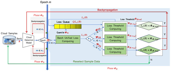
Figure 2.
The pipeline of our proposed CurriCloud. The gray regions represent the full-sample initialization phase and full-sample fine-tuning phase , while the blue region denotes the dynamic curriculum scheduling.
CurriCloud adopts a three-phase training protocol: (1) full-sample initialization phase (), (2) dynamic curriculum scheduling phase (), and (3) full-sample fine-tuning phase ().
During , all samples are randomly selected to establish fundamental feature representations. Phase implements a three-stage (, , and ) curriculum learning strategy that follows a sample difficulty-increasing pattern, dynamically selecting training samples based on their loss values, gradually enhancing the model’s detection capability. The final phase reverts to full random sampling to eliminate potential selection bias.
Phase employs three core components for sample difficulty assessment and selection: (1) sample loss computation using Unified Batch Loss (). is formulated as a weighted summation of classification loss, localization loss, and auxiliary loss; it is used to calculate the loss of the currently selected batch, serving as a direct indicator of sample difficulty, and higher values of correspond to more challenging samples; (2) a FIFO-based loss sliding window queue , which maintains the loss values of the most recent w batches; and (3) sample selection threshold calculation. is derived from the -quantile of , determining whether to retain samples for backpropagation. Phases , , and employ distinct thresholds to progressively include harder samples, progressively adjusting sample selection strategies according to the model’s evolving capabilities, and enabling a step-by-step learning process from easy to hard ground-based cloud samples.
Phase reverts to full random sampling to eliminate prior curriculum learning biases. This unfiltered approach ensures comprehensive parameter space exploration while retaining robust features from earlier phases.
3.3. Sample Difficulty Assessment and Selection
3.3.1. Unified Batch Loss
Easy samples are ones whose correct output can be easily predicted. Samples are tied together through the parameters of the detection models (e.g., YOLOs, DETRs) in the objective function. As a result, no sample is independently judged as easy [36]. Rather, a set of samples is deemed easy only if there exists a model parameter configuration that yields small training loss values for the batch of samples [36]. We propose a Unified Batch Loss (UBL) to serve as a dynamic difficulty metric for sample batch evaluation. The UBL is solely used for assessing batch sample difficulty and does not participate in gradient backpropagation.
Let B denote a training batch of N samples. The total loss for the batch B is defined as Equation (2):
where is the classification loss, measuring the discrepancy between predicted and ground-truth cloud class labels; denotes the localization loss, which quantifies spatial deviations between predicted and ground-truth cloud bounding boxes; and represents auxiliary losses (whose specific functions vary across different object detectors). The coefficients , , are weighting parameters that can be either fixed or dynamically adjusted during the training process. If no auxiliary tasks are present, defaults to 0.
The UBL is calculated using the training loss of the employed detection model. For example, when using models such as YOLOv10 for cloud detection, the UBL incorporates a weighted combination of Focal Loss (to resolve sample imbalance in complex cloud backgrounds), CIoU Loss (for object localization), and DFL Loss (for distribution-focused localization). When applying detectors like RT-DETR for ground-based cloud detection, the UBL integrates VFL Loss (to address inter-class similarity and intra-class variation), Bounding Box Loss, and GIoU Loss (for robust localization of diverse cloud patterns). Additional auxiliary losses are incorporated in the UBL to quantify ground-based cloud sample difficulty.
3.3.2. Loss Sliding Window Queue
The loss sliding window queue is used to monitor the training loss distribution in real-time. The sliding window design adheres to the local consistency hypothesis [48] (where recent loss distributions reflect the model’s current capability), suggesting that limiting the memory length helps balance the model’s sensitivity to recent data and the stability of historical information. It maintains the most recent w batches of loss values relative to the current batch B, represented as , where is defined in Equation (3).
operates as a First-In-First-Out (FIFO) queue, where its elements are dynamically updated during training. Here, w represents the queue length, as illustrated in Figure 3.
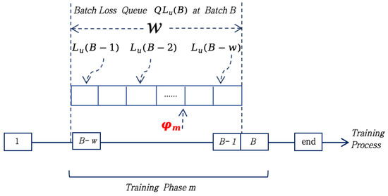
Figure 3.
The loss sliding window queue. The arrow below indicates that the value at this position in the queue is .
The window size w is determined through three key considerations. First, a short window enables rapid adaptation to model performance fluctuations and effectively smooths anomalies caused by challenging samples, making it particularly suitable for architectures with fast convergence, such as YOLO. Conversely, a long window is better suited for models like Transformers, which rely on long-term historical information, as it reduces sensitivity to noise. Additionally, the queue operations ensure computational efficiency, offering a significant advantage over full-loss sorting approaches, where represents the total number of training batches. These factors collectively ensure an optimal balance between adaptability, noise resilience, and computational performance.
3.3.3. Dynamic Loss Threshold
The dynamic loss threshold determines whether to retain the current sample’s training results for backpropagation. It is computed based on the loss sliding window queue values of the current batch B and the loss threshold quantile corresponding to the training phase m (as illustrated in Figure 3), as expressed in Equation (4):
where represents the -quantile operator applied to . Backpropagation is performed when ; otherwise, the sample is re-selected.
The dynamic loss threshold is theoretically equivalent to the dynamic regularization method in online learning [48], ensuring the curriculum pacing remains aligned with the model’s current capabilities. As performance improves, the threshold dynamically decreases following the downward shift of the loss distribution, maintaining an optimal challenge level.
The staged threshold design follows the Self-Paced Learning principle of progressive difficulty, enabling curriculum-based adaptation. The threshold quantile parameter is calibrated according to WMO’s cloud difficulty spectrum [6], accounting for loss variations between cloud types (e.g., high-confidence cirrus vs. low-contrast stratus). This ensures adaptive sample selection aligned with both model capability and meteorological complexity.
3.4. Loss-Based Dynamic Curriculum Learning Scheduling
CurriCloud dynamically schedules training samples using the loss window queue and the adaptive threshold .
CurriCloud adopts a three-phase training protocol: full-sample initialization (), dynamic curriculum scheduling () and full-sample fine-tuning (). Each phase m is formally defined as Equation (5):
where denotes the epoch range, and represents the phase-specific quantile threshold for sample difficulty selection.
The CurriCloud training protocol algorithm (Algorithm 1) is as follows:
Phase (Full-sample Initialization) employs unfiltered training on the complete dataset to establish the representations of the basic characteristics. During this stage, the model learns fundamental cloud characteristics—including texture patterns and morphological shapes—through exhaustive exposure to all available samples. This comprehensive initialization strategy actively mitigates potential sampling bias in early training stages by preventing premature filtering of challenging instances, thereby fostering robust feature embeddings that serve as the basis for subsequent curriculum learning phases.
Phase (Dynamic Curriculum Scheduling) is further divided into three subphases (, and ) with progressively increasing sample difficulty, i.e., . The scheduling protocol operates as follows: First, the Unified Batch Loss is computed for the current batch B. The loss value is then compared against the dynamic threshold . If , the detection model parameters are updated via backpropagation; otherwise, the batch is resampled. Whether or not the model is updated, gets added to the sliding loss queue using FIFO. The protocol implements a phased difficulty progression. Phase employs low thresholds (e.g., ) to incorporate a wider spectrum of sample difficulties, thereby improving model generalization capabilities. Phase employs a moderate threshold (e.g., ) to enhance capability through intermediate samples, while phase applies a high threshold (e.g., ) to focus optimization on challenging cases.
Phase (Full Fine-Tuning) reverts to random sampling across the entire training set, effectively eliminating potential bias introduced by the preceding curriculum learning stages. This final phase serves dual critical purposes: (1) it prevents overfitting that could result from prolonged exposure to filtered samples during the dynamic scheduling phase, and (2) facilitates global convergence by allowing the model to perform unrestricted optimization across all difficulty levels. The unfiltered training paradigm ensures comprehensive exploration of the parameter space, while maintaining the robust feature representations developed during earlier phases.
CurriCloud demonstrates three fundamental improvements over conventional approaches: (1) inherent noise robustness through loss distribution-based difficulty estimation; (2) architectural universality via UBL that bridges CNN-Transformer optimization gaps; and (3) meteorologically interpretable thresholds aligned with WMO standards—notably when , the system automatically focuses on cirrus fibratus differentiation, replicating expert training progression through its dynamic curriculum.
| Algorithm 1 CuriCloud: Ground-based Cloud Detection Model Training |
| Require: Ground-based dataset , training phases and , loss quantiles and , batch size B, loss sliding window queue width w Ensure: Ground-based cloud detection model Phase : Full-sample initialization for training epoch in Phase do end for Initialize loss sliding window queue Phase : Dynamic curriculum scheduling for training epoch in Phase [divided into , and ] do if then end if Update loss sliding window queue end for Phase : Full-sample fine-tuning for training epoch in Phase do end for return model |
4. Experiments
To validate the effectiveness of the CurriCloud strategy, we conducted comprehensive evaluations using three representative detectors on our ALPACLOUD dataset: (1) YOLOv10s (https://github.com/THU-MIG/yolov10) (accessed on 22 January 2025) representing modern CNN-based architectures with optimized gradient flow; (2) RT-DETR-R50 (https://github.com/lyuwenyu/RT-DETR) (accessed on 22 January 2025), exemplifying Transformer-based real-time detection; and (3) Ultra-Light-Fast-Generic-Face-Detector-1MB (ULFG-FD, https://github.com/Linzaer/Ultra-Light-Fast-Generic-Face-Detector-1MB/) (accessed on 10 November 2024), an SSD [49] derived ultra-lightweight detector, highlighting anchor-based designs under extreme model compression. This selection spans the full spectrum of contemporary detection paradigms (CNNs, Transformers, and traditional single-shot detectors), enabling rigorous assessment of CurriCloud’s adaptive training across: (1) multi-scale feature fusion (YOLOv10s), (2) attention-based query mechanisms (RT-DETR-R50), and (3) predefined anchor box systems (ULFG-FD).
4.1. Datasets
We evaluate our method on the ALPACLOUD dataset, as illustrated in Figure 4. The ALPACLOUD dataset comprises 1786 original high-resolution (1068 × 756 pixels) ground-based cloud images collected across seven Chinese provinces representing distinct climate zones: coastal regions (Hainan, Guangdong) with tropical monsoon climates, northern areas (Beijing, Hebei, Liaoning) featuring temperate continental climates, transitional zones (Shandong) with mixed humid subtropical conditions, and mountainous terrain (Fujian) exhibiting high-altitude microclimates. The images were captured between 2023 and 2025 using professional-grade digital digital camera sensors.
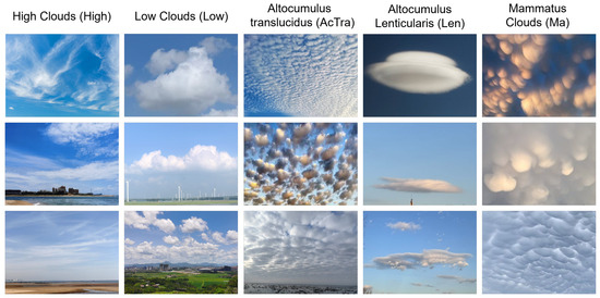
Figure 4.
Some representative cloud types in ALPACLOUD.
Following WMO standards, the images were annotated with five cloud categories, as showcased in Figure 4: (1) high clouds (High, 37.07%), (2) low clouds (Low, 46.14%), (3) Altocumulus translucidus (Ac tra, 5.94%), (4) Altocumulus lenticularis (Ac len, 5.38%), and (5) mammatus clouds (Ma, 5.49%). This composition ensures comprehensive coverage of cloud morphological variations while incorporating challenging ground backgrounds common in operational nowcasting scenarios.
The statistical distribution closely mirrors natural cloud-type occurrence patterns, with high and low clouds dominating in frequency. While specialized formations like Altocumulus translucidus, Altocumulus lenticularis, and mammatus clouds exhibit lower incidence rates, their inclusion significantly enhances model generalizability through spectral–spatial diversity infusion; this proves particularly critical for enhancing nowcasting accuracy of high-impact meteorological phenomena. Cloud classification and morphological features are illustrated in Table 1.

Table 1.
Class descriptions of cloud types in ALPACLOUD.
To address class imbalance in the World Meteorological Organization (WMO) cloud classification standards, we adopted stratified sampling to partition the dataset (training set 70.89%, validation set 6.94%, test set 22.17%). For rare cloud types like mammatus clouds, we applied 3× data augmentation using geometric transformations (random cropping, rotation, scaling) and color jittering (brightness/contrast/saturation adjustment). Similarly, special cloud types such as altocumulus lenticularis were augmented with 3× combined transformations including geometric operations and color adjustments. The annotation process employed the LabelImg toolbox with rigorous quality control: connected homogeneous clouds without obstacle occlusion are treated as a single target if their bodies are continuous, and as two separate targets if their bodies are discontinuous.
4.2. Evaluation Metrics
In our work, we employ mAP50, precision, and recall as the evaluation criteria to evaluate the detection performance of our method. Considering the fractal structure and fuzzy edges of cloud boundaries, these metrics are adaptively adjusted to accommodate the inherent uncertainties in cloud morphology. Precision and recall are respectively defined in Equations (6) and (7):
where TP (True Positive) refers to the correctly detected cloud areas, both locations and categories. FP (False Positive) represents the background areas misclassified as cloud or the incorrect cloud category, and FN (False Negative) indicates the undetected real cloud areas.
Based on Equations (6) and (7), we can obtain definitions for the Average Precision (AP) and Mean Average Precision (mAP), as shown in Equations (8) and (9):
AP (Average Precision) is the area under the precision–recall curve for a single class. It integrates precision across all recall levels.
The mAP50 (mean average precision at MAIoU = 0.5) provides the average value of the AP for each category, with denoting the number of cloud types in the whole dataset, where MAIoU (meteorologically adaptive Intersection over Union) is defined as (10):
where is the predicted box, and is the ground truth box. Based on , we propose a meteorologically adaptive lenient-matching strategy that incorporates (1) One-to-Many Matching where a single prediction box can contain multiple homogeneous ground truth (GT) clouds, with TP counts based on the number of valid prediction boxes; and (2) Many-to-One Matching where multiple predictions can match to a single GT cloud, with only the first matched prediction counted as TP and subsequent matches not penalized as FP. Figure 5 shows examples of the calculation of the metrics.
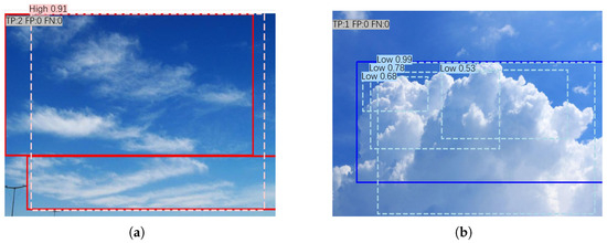
Figure 5.
Examples of CurriCloud annotations and results (dark colors represent ground truth boxes, light colors represent predicted boxes, and the same color scheme indicates the same category). In (a), when a prediction box encloses multiple cirrus GTs, each unmatched GT independently increments the TP count. (b) demonstrates that substructure detections within cumulus layers contribute only 1 TP without triggering FPs.
As shown in Figure 5a, when a prediction box encloses multiple cirrus GTs, each unmatched GT independently increments the TP count. Conversely, Figure 5b demonstrates that substructure detections within cumulus layers contribute only 1 TP without triggering FPs. This strategy preserves critical capabilities for tracking cloud system movements (via bounding box coordinates) while significantly relaxing boundary precision requirements, better aligning with meteorological operational needs.
4.3. Implementation Details
Our evaluation was carried out on the ALPACLOUD dataset using YOLOv10 (CNN-based), RT-DETR (transformer-based) and ULFG-FD (anchor-based). All experiments were performed on a dedicated Ubuntu 22.04 computer equipped with an NVIDIA GeForce RTX 4090 GPU and Intel Core i9-14900HX processor, utilizing Python 3.9.21 and CUDA 12.6 for accelerated computing.
To address the distinct capabilities of different detection models and the specific challenges in cloud detection, the experiment employed customized loss weight configurations for each architecture: YOLOv10s was configured with classification (), localization (), and auxiliary loss weights () to prioritize cloud category discrimination, RT-DETR-R50 used , , to leverage its transformer architecture’s strength in spatial relationships, and ULFG-FD adopted , with configuration reflecting its anchor-based design’s balanced approach to classification and localization without auxiliary tasks. All loss weighting parameters , , and in UBL for the models (YOLOv10s, RT-DETR-R50, and ULFG-FD) remained unchanged during CurriCloud training.
The sample batch size was set to 16 for YOLOv10s, 8 for RT-DETR-R50, and 24 for ULFG-FD.
CurriCloud settings for different detector models are illustrated in Table 2.
Table 2.
CurriCloud settings for different detectors.
We employed stochastic gradient descent (SGD) optimization for YOLOv10s and ULFG-FD, adaptive moment estimation (Adam) for RT-DETR-R50, maintaining consistent optimizer choices between conventional and CurriCloud training regimes to ensure fair comparison.
4.4. Results
Comparative experimental results demonstrated that CurriCloud consistently outperformed conventional training methods in mAP50 performance metrics across all architectures.
The experimental results are presented in Table 3.
Table 3.
Performance comparison between conventional training and CurriCloud on ALPACLOUD dataset (mAP50, precision, and recall reported in decimal format). Bold number indicates exceeding the model baseline (Conventional).
The experimental results demonstrate that CurriCloud consistently enhances detection performance across all architectures, with notable improvements observed for YOLOv10s (+3.1% mAP50, 0.800→0.831) where its dynamic difficulty adaptation effectively addresses the model’s sensitivity to complex cloud formations. Most notably, ULFG-FD achieves a 11.4% relative improvement (0.442→0.556), highlighting the framework’s particular efficacy for single-shot detectors in meteorological applications. The Transformer-based RT-DETR-R50 maintains its high baseline performance with a 1.2% gain (0.863→0.875), confirming stable integration with attention mechanisms. Precision–recall characteristics diverge by architecture: (1) YOLOv10s shows increased precision (0.943→0.955) with reduced recall (0.820→0.787), suggesting optimized confidence calibration; (2) ULFG-FD maintains comparable precision (0.878%→0.835) while improving recall (0.557→0.593); and (3) RT-DETR-R50 sustains exceptional precision (0.977→0.975) while substantially increasing recall (0.780→0.813). These findings validate CurriCloud’s robust adaptability across diverse detection paradigms in ground-based cloud observation systems.
It should be particularly noted that the precision–recall trade-off was observed in YOLOv10s. It primarily stems from its anchor-free architecture’s inherent reliance on high-confidence features. During early training phases, the dynamic threshold preferentially selects high-confidence cloud samples, effectively reducing false positives from complex backgrounds while temporarily neglecting detection of marginal cloud formations, leading to decreased recall. Meteorological analysis reveals this recall reduction primarily affects thin cirrus clouds (WMO classification Ci fibratus) at image peripheries—these are intentionally deprioritized in initial phases as they minimally impact nowcasting operations.
Figure 6 presents a comparative visualization between CurriCloud’s detection results and conventional training regimes.
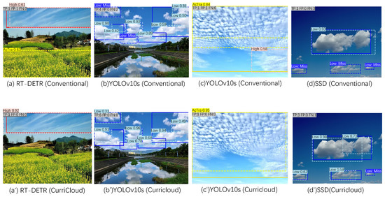
Figure 6.
Visualization of test results on ALPACLOUD.
In case (a), the baseline RT-DETR-R50 model erroneously classified a rapeseed field as Altocumulus translucidus; this error was successfully resolved through CurriCloud. Case (b) shows dense low-cloud scenarios; the baseline YOLOv10s exhibited two false negatives, but CurriCloud successfully recalled all of them. Case (c) addressed the spectral similarity between Altocumulus translucidus and cirrostratus clouds; the baseline YOLOv10s model misidentified part of it as high clouds, but this error was eliminated by CurriCloud. In case (d), while the baseline ULFG-FD approach missed three low-cloud instances, CurriCloud reduced omission errors to a single instance.
4.5. Ablation Study
We conducted comprehensive experiments to evaluate two core hyperparameters governing CurriCloud’s adaptive behavior: (1) the loss sliding window queue length (w), which determines the memory capacity for tracking recent batch losses and stabilizes difficulty estimation, and (2) the phase-specific threshold quantiles that systematically increase sample difficulty during the dynamic curriculum stage. All experiments maintained consistent settings, including architecture-specific optimizers (SGD for CNNs/Adam for Transformers) and fixed mini-batch sizes (YOLOv10s: 16, ULFG-FD: 20, RT-DETR-R50: 4) on the ALPACLOUD dataset.
Table 4 presents the parameter ablation study of CurriCloud on the ALPACLOUD, evaluating different queue lengths (w) and threshold quantiles .
Table 4.
Parameter ablation study of CurriCloud with varying queue lengths (w) and threshold quantiles , , and on ALPACLOUD. Bold number indicates exceeding the model baseline (Conventional), and red number represents the best performance of the parameter in this model.
The nomenclature for CurriCloud configurations follows the pattern ‘lossABCDE’, where ‘loss’ indicates dynamic loss-based sample difficulty assessment and curriculum scheduling; the first two symbols (‘AB’) specify the loss sliding window queue length w, where ‘–’ represents not using the loss sliding window queue; and the subsequent three symbols (‘CDE’) represent Phase 1, Phase 2, and Phase 3 threshold quantiles scaled by 10, respectively.
The ablation study results in Table 4 demonstrate distinct optimization patterns for each architecture. Sensitivity analysis and implementation recommendations are as followings.
- Loss Sliding Window Queue Length () AnalysisThe queue length (w) fundamentally governs three critical aspects of the curriculum learning process: (1) temporal granularity, where smaller values () enable rapid difficulty adaptation to dynamic cloud patterns; (2) estimation stability, as larger windows (–40) reduce threshold volatility through extended loss observation; and (3) memory–accuracy trade-off, where achieves the peak mAP50 of 0.875 with significantly lower memory usage than , making it ideal for operational deployment in ground-based cloud observation systems. The ablation of the loss sliding window leads to substantial performance drops for CurriCloud on YOLOv10s and RT-DETR-R50 benchmarks (YOLOv10s:loss–579 and loss–789, RT-DETR-R50:loss–789) relative to equivalent-threshold baselines, confirming its contribution to model improvement.
- Phase-Specific Threshold AnalysisPhase-specific threshold quantiles (, , ) in CurriCloud’s dynamic curriculum learning stage () were designed to progressively increase the difficulty of the sample through three pedagogically structured subphases: Phase employs for a wide coverage of difficulty to establish robust feature representations, Phase transitions to for intermediate difficulty optimization, and Phase focuses on challenging samples with .
This graduated approach yields architecture-specific benefits: (1) For YOLOv10s, the [0.5, 0.7, 0.9] configuration achieves optimal mAP50 (0.821) and precision (0.955) with , suggesting early-phase low threshold () helps maintain feature diversity, and late-phase high threshold () effectively filters outliers, demonstrating CNNs’ preference for explicit difficulty staging; (2) RT-DETR-R50 performs best (mAP50 = 0.875, recall = 0.813) using [0.7, 0.8, 0.9] and , reflecting that transformer architectures benefit from earlier focus on medium-difficulty samples and gradual threshold increase (0.7→0.8→0.9) matches self-attention’s learning dynamics; while (3) ULFG-FD maintains stable performance (mAP50 0.554–0.556) across –20 with , showing simpler detectors’ robustness to parameter variations. The systematic progression proves to be particularly effective for cloud differentiation.
Computational cost or processing efficiency analysis: The experiment results demonstrate that CurriCloud significantly improves detection performance with minimal training overhead: YOLOv10s achieves +2.1% mAP50 with only 17% longer training (1:55→2:15); RT-DETR-R50 gains +1.2% mAP50 at a 24% time cost (5:39→7:04).
The increased training computational overhead primarily stems from three aspects: sample resampling represents the most significant time cost, while sliding window queue updates and quantile threshold computing account for less processing time and consume less memory, since the sliding window update operates in constant time, i.e., , ensuring high computational efficiency during batch processing. The quantile threshold calculation requires time complexity, where w represents the window size. This complexity arises from the sorting operations necessary for accurate quantile estimation. The parameter count, FLOPs, and inference time of CurriCloud remain identical to those of the original object detection model, as CurriCloud does not modify the model architecture.
4.6. Comparative Study
We compared CurriCloud with two curriculum learning approaches: the static difficulty metric-based Stastic-CL and another curriculum learning approach SPCL [40] (which combines static metrics with training loss for sample difficulty definition) on the ALPACLOUD dataset. For fair comparison, only the sample difficulty assessment method was modified in Stastic-CL, while all other settings remained identical to CurriCloud. The curriculum learning implementation for SPCL followed the method described in [40].
(1) Sample difficulty assessment in Stastic-CL.
The sample batch difficulty is defined as the weighted sum:
where N represents sample batch size, and the weighting coefficients (0.3, 0.4) reflect the relative importance of each dimension, empirically determined through psychophysical experiments. Calculation methods for each component are detailed below.
Category Complexity ():
where represents distinct cloud types (e.g., cirrus, cumulus). Each type contributes 20 points, capped at 100 points (i.e., ≥5 cloud types yield maximum score).
Target Size Ratio ():
where is the area of the i-th bounding box and is the total image area. The sixth-order power function amplifies the difficulty contribution of small targets () while suppressing interference from minuscule targets.
(2) Sample difficulty assessment in SPCL.
The sample difficulty is defined as the weighted sum:
where UBL is defined as the same as Curricloud. The weighting coefficient is evaluated with loss quantile thresholds varied as 0.2, 0.1, and 0.05, respectively.
We implemented the three-phase training strategy as CurriCloud for Stastic-CL and SPCL, with the same threshold combinations: (1) thresholds (0.5/0.7/0.9) for YOLOv10s, and (2) thresholds (0.7/0.8/0.9) for RT-DETR-R50. The setting of the loss sliding window queue is also the same as CurriCloud. The results are shown in Table 5.
Table 5.
Performance comparison with identical hyperparameters across all methods. Bold number indicates exceeding the model baseline, and red number represents the best performance.
The experimental results in Table 5 demonstrate CurriCloud’s consistent superiority over both Static CL and SPCL across all evaluation metrics, with YOLOv10s achieving a 1.9% and 1.6% higher mAP50 (0.831 vs. 0.802 and 0.805) and RT-DETR-R50 showing a 1.8% and 3.0% improvement (0.875 vs. 0.857 and 0.845). This performance advantage stems from CurriCloud’s integration of real-time loss analysis through sliding windows and meteorologically informed phased thresholds, which effectively addresses the fundamental limitations of conventional approaches: unlike SPL’s reliance on instantaneous loss values that often misclassify morphologically complex stratocumulus as hard samples due to localization loss spikes while underestimating the diversity of fragmented clouds, and SPCL’s dependence on static physical metrics like cloud size that fail to altocumulus variations, CurriCloud dynamically adapts to cloud detection challenges by progressively adjusting sample selection, matching WMO classification standards while maintaining balanced precision–recall characteristics.
Figure 7 presents a comparative analysis of loss–epoch curves for the five training regimes on YOLOv10s and RT-DETR-R50 architectures.
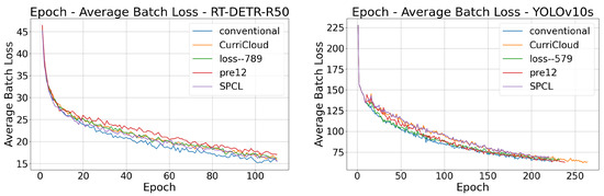
Figure 7.
Loss–epoch curves and precision–recall (P-R) performance for the five training regimes on YOLOv10s and RT-DETR-R50 architectures.
Due to the fact that CurriCloud skips some batches, the number of samples within each epoch is reduced. When the horizontal axis is epoch, the descent rate of the loss curve slows down. However, the loss when achieving the best effect does not change significantly compared with that of the conventional model. Figure 8 is the precision–recall (PR) curves comparing five training regimes—conventional (baseline), CurriCloud (proposed), and Static-CL—across three object detection architectures.
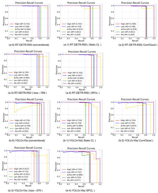
Figure 8.
(P-R) performance for the three strategies on YOLOv10s and RT-DETR-R50 architectures.
As shown in Figure 8, for RT-DETR-R50, CurriCloud improves the AP of high clouds from 0.741 to 0.789 and the AP of low clouds from 0.768 to 0.798, with almost no change in the AP of other classes, thus enhancing the recognition performance of common cloud types. For YOLOv10s, although the APs of high clouds and low clouds decrease slightly, CurriCloud increases the AP of Altocumulus translucidus from 0.785 to 0.874 and the AP of mammatus clouds from 0.901 to 1.000, improving the recognition performance of rare cloud types. By contrast, the performance improvement of Static CL (pre12-579) and SPCL is less pronounced. In summary, CurriCloud demonstrates distinct improvements in recognizing common and rare cloud types across different models, outperforming Static CL (pre12-579) and SPCL in performance enhancement.
4.7. Integration Recommendations for Meteorological Systems
- CurriCloud Parameter RecommendationsFor optimal deployment in ground-based cloud systems, we recommend (1) CNN architectures (YOLOv10s) adopt with a threshold scheme [0.5, 0.7, 0.9] to achieve high precision; (2) transformer architectures (RT-DETR-R50) use with [0.7, 0.8, 0.9] for high recall; and (3) legacy models (ULFG-FD) employ flexible –20 with [0.5, 0.7, 0.9]. Scenario-specific tuning suggests for short-term nowcasting (capturing rapid cloud evolution) and for climate monitoring (reducing false cirrus detection). Hardware constraints dictate for edge devices (40% memory savings) and for cloud servers, all validated on ALPACLOUD’s diverse meteorological data.
- Recommendations for optimal deployment in meteorological systemsFor optimal deployment of the CurriCloud model in operational meteorological systems, we propose the following architecture-specific integration strategies: (1) Edge computing devices at weather stations should employ the ONNX Runtime with C++ implementation to achieve low-latency processing while minimizing computational overhead. (2) Cloud-based numerical weather prediction systems are advised to adopt REST API encapsulation (Python/Java) for enhanced scalability and interoperability with existing forecasting pipelines. (3) High-performance real-time monitoring applications should leverage TensorRT optimization with CUDA acceleration. For field deployment scenarios, we recommend implementing an automated pipeline where ground-based cloud imagery is streamed to the CurriCloud model, which subsequently outputs structured JSON data containing georeferenced cloud classifications for integration with meteorological databases and visualization systems. This tiered approach ensures computational efficiency while maintaining the model’s improvement in detection accuracy across diverse cloud regimes.
5. Conclusions
This study presents CurriCloud, a dynamic curriculum learning framework that optimizes cloud detection by addressing sample difficulty variation. Its key innovation lies in the self-adaptive difficulty assessment, which ensures alignment between sample difficulty and the model’s evolving capability while maintaining compatibility with mainstream detectors (YOLOv10s, RT-DETR-R50, and ULFG-FD). The meteorology-guided phase-wise scheduling strategy proves particularly effective for fine-grained cloud type discrimination, offering immediate value for automated meteorological observation. Parameter studies further demonstrate adaptable configuration strategies and superior performance across detector architectures. Future work will integrate more efficient meteorological cloud imagery difficulty metrics with adaptive loss functions, investigating enhanced cloud detection efficacy through curriculum learning strategies.
Author Contributions
Methodology, T.Q.; writing—original draft, T.Q.; writing—review and editing, Y.H., J.W., and T.Q.; supervision, Y.H.; project administration, Y.H. All authors have read and agreed to the published version of the manuscript.
Funding
This research received no external funding.
Data Availability Statement
Our code is available at: https://github.com/qitianhong111/CurriCloud (accessed on 10 May 2025). The raw data supporting the conclusions of this article will be made available by the authors on request.
Acknowledgments
We extend our sincere gratitude to Wenfei Li, Xiaoqiang Mo, Haote Yang, and Zongqi Duan at Ocean University of China for their invaluable contributions to dataset curation and annotation. Special thanks are also due to Jian Zhang, Gubang Xu, and Xu Cheng from the University of Science and Technology Beijing for their expertise in model training.
Conflicts of Interest
The authors declare no conflicts of interest.
Abbreviations
The following abbreviations are used in this manuscript:
| WMO | The World Meteorological Organization |
| CNN | Convolutional neural network |
| CL | Curriculum learning |
| SPL | Self-paced Learning |
| SPCL | Self-paced curriculum leaning |
| UBL | Unified batch loss |
| ULFG-FD | Ultra-Light-Fast-Generic-Face-Detector-1MB |
References
- Li, S.; Wang, M.; Shi, M.; Wang, J.; Cao, R. Leveraging Deep Spatiotemporal Sequence Prediction Network with Self-Attention for Ground-Based Cloud Dynamics Forecasting. Remote Sens. 2025, 17, 18. [Google Scholar] [CrossRef]
- Lu, Z.; Zhou, Z.; Li, X.; Zhang, J. STANet: A Novel Predictive Neural Network for Ground-Based Remote Sensing Cloud Image Sequence Extrapolation. IEEE Trans. Geosci. Remote Sens. 2023, 61, 4701811. [Google Scholar] [CrossRef]
- Wei, L.; Zhu, T.; Guo, Y.; Ni, C.; Zheng, Q. Cloudprednet: An ultra-short-term movement prediction model for ground-based cloud image. IEEE Access 2023, 11, 97177–97188. [Google Scholar] [CrossRef]
- Deng, F.; Liu, T.; Wang, J.; Gao, B.; Wei, B.; Li, Z. Research on Photovoltaic Power Prediction Based on Multimodal Fusion of Ground Cloud Map and Meteorological Factors. Proc. CSEE 2025. Available online: https://link.cnki.net/urlid/11.2107.TM.20250220.1908.019 (accessed on 21 February 2025).
- Rachana, G.; Satyasai, J.N. Cloud Detection in Satellite Images with Classical and Deep Neural Network Approach: A Review. Multimed. Tools Appl. 2022, 81, 31847–31880. [Google Scholar] [CrossRef]
- World Meteorological Organization. International Cloud Atlas (WMO-No.407); WMO: Geneva, Switzerland, 2017. [Google Scholar]
- Neto, S.L.M.; Wangenheim, R.V.; Pereira, R.B.; Comunello, R. The Use of Euclidean Geometric Distance on RGB Color Space for the Classification of Sky and Cloud Patterns. J. Atmos. Ocean. Technol. 2010, 27, 1504–1517. [Google Scholar] [CrossRef]
- Liu, S.; Wang, C.H.; Xiao, B.H.; Zhang, Z.; Shao, Y.X. Salient Local Binary Pattern for Ground-Based Cloud Classification. Acta Meteorol. Sin. 2013, 27, 211–220. [Google Scholar] [CrossRef]
- Cheng, H.Y.; Yu, C.C. Block-Based Cloud Classification with Statistical Features and Distribution of Local Texture Features. Atmos. Meas. Tech. 2015, 8, 1173–1182. [Google Scholar] [CrossRef]
- Wang, C.Y.; Liao, H.Y.M. YOLOv1 to YOLOv10: The Fastest and Most Accurate Real-Time Object Detection Systems. arXiv 2024, arXiv:2405.14458. [Google Scholar] [CrossRef]
- Lv, W.; Zhao, Y.; Xu, S.; Wei, J.; Wang, G.; Cui, C.; Du, Y.; Dang, Q.; Liu, Y. DETRs Beat YOLOs on Real-Time Object Detection. In Proceedings of the IEEE/CVF Conference on Computer Vision and Pattern Recognition (CVPR), Seattle, WA, USA, 16–22 June 2024; pp. 16965–16974. [Google Scholar] [CrossRef]
- Zhao, S.J.; Chen, H.; Zhang, X.L.; Xiao, P.F.; Bai, L.; Ouyang, W.L. RS-Mamba for large remote sensing image dense prediction. IEEE Trans. Geosci. Remote Sens. 2024, 62, 5633314. [Google Scholar] [CrossRef]
- Li, Y.K.; Zhu, W.; Wu, J.; Zhang, R.X.; Xu, X.Y. DBSANet: A dual-branch semantic aggregation network integrating CNNs and transformers for landslide detection in remote sensing images. Remote Sens. 2025, 17, 807. [Google Scholar] [CrossRef]
- Wang, Z.T.; Cao, X.Z.; Chen, Y.S.; Wang, G.P. SAIP-Net: Enhancing remote sensing image segmentation via spectral adaptive information propagation. arXiv 2025, arXiv:2504.16564. [Google Scholar] [CrossRef]
- Chand, K.V.; Ashwini, K.; Yogesh, M.; Jyothi, G.P. Object detection in remote sensing images using YOLOv8. In Proceedings of the 2024 International Conference on Integrated Intelligence and Communication Systems (ICIICS), Kalaburagi, India, 22–23 November 2024. [Google Scholar] [CrossRef]
- Redmon, J.; Divvala, S.; Girshick, R.; Farhadi, A. You Only Look Once: Unified, Real-Time Object Detection. In Proceedings of the IEEE Conference on Computer Vision and Pattern Recognition (CVPR), Las Vegas, NV, USA, 27–30 June 2016; pp. 779–788. [Google Scholar] [CrossRef]
- Wang, A.; Chen, H.; Liu, L.H.; Chen, K.; Lin, Z.J.; Han, J.G.; Ding, G.G. YOLOv10: Real-Time End-to-End Object Detection. In Proceedings of the Advances in Neural Information Processing Systems 37 (NeurIPS 2024), Vancouver, Canada, 10–15 December 2024; pp. 107984–108011. [Google Scholar] [CrossRef]
- Carion, N.; Massa, F.; Synnaeve, G.; Usunier, N.; Kirillov, A.; Zagoruyko, S. End-to-End Object Detection with Transformers. In Computer Vision—ECCV 2020; Springer: Cham, Switzerland, 2020; pp. 213–229. [Google Scholar] [CrossRef]
- Wang, S.; Chen, Y. Ground Nephogram Object Detection Algorithm Based on Improved Loss Function. Comput. Eng. Appl. 2022, 58, 169–175. [Google Scholar] [CrossRef]
- Hu, J.; Wei, Y.; Chen, W.; Zhi, X.; Zhang, W. CM-YOLO: Typical Object Detection Method in Remote Sensing Cloud and Mist Scene Images. Remote Sens. 2025, 17, 125. [Google Scholar] [CrossRef]
- Zhou, Z.; Zhang, F.; Xiao, H.; Wang, F.; Hong, X.; Wu, K.; Zhang, J. A Novel Ground-Based Cloud Image Segmentation Method by Using Deep Transfer Learning. IEEE Geosci. Remote Sens. Lett. 2022, 19, 4004705. [Google Scholar] [CrossRef]
- Wang, M.; Zhuang, Z.H.; Wang, K.; Zhang, Z. Intelligent Classification of Ground-Based Visible Cloud Images Using a Transfer Convolutional Neural Network and Fine-Tuning. Opt. Express 2021, 29, 150455. [Google Scholar] [CrossRef]
- Bengio, Y.; Louradour, J.; Collobert, R.; Weston, J. Curriculum Learning. In Proceedings of the 26th Annual International Conference on Machine Learning, Montreal, QC, Canada, 14–18 June 2009; pp. 41–48. [Google Scholar] [CrossRef]
- Soviany, P.; Ionescu, R.T.; Rota, P.; Sebe, N. Curriculum Learning: A Survey. Int. J. Comput. Vis. 2022, 130, 1526–1565. [Google Scholar] [CrossRef]
- Wang, X.; Chen, Y.; Zhu, W. A Survey on Curriculum Learning. IEEE Trans. Pattern Anal. Mach. Intell. 2021, 44, 4555–4576. [Google Scholar] [CrossRef]
- Chen, J.N.; Lu, Y.Y.; Yu, Q.H.; Luo, X.D.; Adeli, E.; Wang, Y.; Lu, L.; Yuille, A.L.; Zhou, Y.Y. TransUNet: Transformers Make Strong Encoders for Medical Image Segmentation. In Proceedings of the IEEE/CVF Conference on Computer Vision and Pattern Recognition (CVPR 2021), Nashville, TN, USA, 19–25 June 2021; Volume 1, pp. 12557–12567. [Google Scholar] [CrossRef]
- Liu, S.; Duan, L.L.; Zhang, Z.; Cao, X.Z.; Durrani, T.S. Ground-Based Remote Sensing Cloud Classification via Context Graph Attention Network. IEEE Trans. Geosci. Remote Sens. 2022, 60, 5602711. [Google Scholar] [CrossRef]
- Chen, J.N.; Lu, Y.Y.; Yu, Q.H.; Luo, X.D.; Adeli, E.; Wang, Y.; Lu, L.; Yuille, A.L.; Zhou, Y.Y. AAformer: Auto-Aligned Transformer for Person Re-Identification. IEEE Trans. Neural Netw. Learn. Syst. 2024, 35, 17307–17317. [Google Scholar] [CrossRef]
- Zhang, X.; Jia, K.B.; Liu, J.; Zhang, L. Ground Cloud Image Recognition and Segmentation Technology Based on Multi-Task Learning. Meteorol. Mon. 2023, 49, 454–466. [Google Scholar] [CrossRef]
- Khan, M.; Hamila, R.; Menouar, H. CLIP: Train Faster with Less Data. In Proceedings of the International Conference on Big Data and Smart Computing (BigComp), Jeju, Republic of Korea, 13–16 February 2023; pp. 34–39. [Google Scholar] [CrossRef]
- Ionescu, R.T.; Alexe, B.; Leordeanu, M.; Popescu, M.; Papadopoulos, D.P.; Ferrari, V. How Hard Can It Be? Estimating the Difficulty of Visual Search in an Image. In Proceedings of the IEEE Conference on Computer Vision and Pattern Recognition (CVPR), Las Vegas, NV, USA, 27–30 June 2016; pp. 2157–2166. [Google Scholar] [CrossRef]
- Shi, M.; Ferrari, V. Weakly Supervised Object Localization Using Size Estimates. In Computer Vision—ECCV 2016; Springer: Cham, Switzerland, 2016; pp. 105–121. [Google Scholar] [CrossRef]
- Soviany, P.; Ionescu, R.T.; Rota, P.; Sebe, N. Curriculum Self-Paced Learning for Cross-Domain Object Detection. Comput. Vis. Image Underst. 2021, 204, 103166. [Google Scholar] [CrossRef]
- Gong, M.; Li, H.; Meng, D.; Miao, Q.; Liu, J. Decomposition-Based Evolutionary Multiobjective Optimization for Self-Paced Learning. IEEE Trans. Evol. Comput. 2019, 23, 288–302. [Google Scholar] [CrossRef]
- Khan, M.A.; Menouar, H.; Hamila, R. LCDNet: A Lightweight Crowd Density Estimation Model for Real-Time Video Surveillance. J. Real Time Image Process. 2023, 20, 29. [Google Scholar] [CrossRef]
- Kumar, M.P.; Packer, B.; Koller, D. Self-Paced Learning for Latent Variable Models. In Proceedings of the 23rd International Conference on Neural Information Processing Systems (NIPS 2010), Vancouver, BC, Canada, 6–9 December 2010; Volume 23, pp. 1189–1197. [Google Scholar]
- Fan, Y.; He, R.; Liang, J.; Hu, B.G. Self-Paced Learning: An Implicit Regularization Perspective. In Proceedings of the AAAI Conference on Artificial Intelligence, San Francisco, CA, USA, 4–9 February 2017; pp. 1877–1883. [Google Scholar] [CrossRef]
- Li, H.; Gong, M.; Meng, D.; Miao, Q. Multi-Objective Self-Paced Learning. In Proceedings of the AAAI Conference on Artificial Intelligence, Phoenix, AZ, USA, 12–17 February 2016; pp. 1802–1808. [Google Scholar] [CrossRef]
- Zhou, S.; Wang, J.; Meng, D.; Xin, X.; Li, Y.; Gong, Y.; Zheng, N. Deep Self-Paced Learning for Person Re-Identification. Pattern Recognit. 2018, 76, 739–751. [Google Scholar] [CrossRef]
- Jiang, L.; Meng, D.; Zhao, Q.; Shan, S.; Hauptmann, A.G. Self-Paced Curriculum Learning. In Proceedings of the AAAI Conference on Artificial Intelligence, Austin, TX, USA, 25–30 January 2015; pp. 2694–2700. [Google Scholar] [CrossRef]
- Ma, F.; Meng, D.; Xie, Q.; Li, Z.; Dong, X. Self-Paced Co-Training. In Proceedings of the 34th International Conference on Machine Learning (ICML), Sydney, Australia, 6–11 August 2017; Volume 70, pp. 2275–2284. [Google Scholar]
- Croitoru, F.A.; Ristea, N.C.; Ionescu, R.T.; Sebe, N. Learning Rate Curriculum. Int. J. Comput. Vis. 2025, 133, 1–23. [Google Scholar] [CrossRef]
- Sinha, S.; Garg, A.; Larochelle, H. Curriculum by Smoothing. Adv. Neural Inf. Process. Syst. 2020, 33, 21653–21664. [Google Scholar] [CrossRef]
- Lin, T.Y.; Goyal, P.; Girshick, R.; He, K.; Dollár, P. Focal Loss for Dense Object Detection. In Proceedings of the IEEE International Conference on Computer Vision (ICCV), Venice, Italy, 22–29 October 2017; pp. 2999–3007. [Google Scholar] [CrossRef]
- Girshick, R. Fast R-CNN. In Proceedings of the IEEE International Conference on Computer Vision (ICCV), Santiago, Chile, 7–13 December 2015; pp. 1440–1448. [Google Scholar] [CrossRef]
- Rezatofghil, H.; Tsoi, N.; Gwak, J.; Sadeghian, A.; Reid, I.; Savarese, S. Generalized Intersection over Union: A Metric and a Loss for Bounding Box Regression. In Proceedings of the IEEE/CVF Conference on Computer Vision and Pattern Recognition (CVPR), Long Beach, CA, USA, 16–20 June 2019; pp. 658–666. [Google Scholar] [CrossRef]
- Allo, N.T.; Indrabayu; Zainuddin, Z. A Novel Approach of Hybrid Bounding Box Regression Mechanism to Improve Convergence Rate and Accuracy. Int. J. Intell. Eng. Syst. 2024, 17, 57–68. [Google Scholar] [CrossRef]
- Hazan, E. Introduction to Online Convex Optimization (Second Edition). arXiv 2023. [Google Scholar] [CrossRef]
- Liu, W.; Anguelov, D.; Erhan, D.; Szegedy, C.; Reed, S.; Fu, C.Y.; Berg, A.C. SSD: Single Shot MultiBox Detector. In Computer Vision—ECCV 2016; Springer: Cham, Switzerland, 2016; pp. 21–37. [Google Scholar] [CrossRef]


Disclaimer/Publisher’s Note: The statements, opinions and data contained in all publications are solely those of the individual author(s) and contributor(s) and not of MDPI and/or the editor(s). MDPI and/or the editor(s) disclaim responsibility for any injury to people or property resulting from any ideas, methods, instructions or products referred to in the content. |
© 2025 by the authors. Licensee MDPI, Basel, Switzerland. This article is an open access article distributed under the terms and conditions of the Creative Commons Attribution (CC BY) license (https://creativecommons.org/licenses/by/4.0/).