HG-Mamba: A Hybrid Geometry-Aware Bidirectional Mamba Network for Hyperspectral Image Classification

Abstract

Deep learning has demonstrated significant success in hyperspectral image (HSI) classification by effectively leveraging spatial–spectral feature learning. However, current approaches encounter three challenges: (1) high spectral redundancy and the presence of noisy bands, which impair the extraction of discriminative features; (2) limited spatial receptive fields inherent in convolutional operations; and (3) unidirectional context modeling that inadequately captures bidirectional dependencies in non-causal HSI data. To address these challenges, this paper proposes HG-Mamba, a novel hybrid geometry-aware bidirectional Mamba network for HSI classification. The proposed HG-Mamba synergistically integrates convolutional operations, geometry-aware filtering, and bidirectional state-space models (SSMs) to achieve robust spectral–spatial representation learning. The proposed framework comprises two stages. The first stage, termed spectral compression and discrimination enhancement, employs multi-scale spectral convolutions alongside a spectral bidirectional Mamba (SeBM) module to suppress redundant bands while modeling long-range spectral dependencies. The second stage, designated spatial structure perception and context modeling, incorporates a Gaussian Distance Decay (GDD) mechanism to adaptively reweight spatial neighbors based on geometric distances, coupled with a spatial bidirectional Mamba (SaBM) module for comprehensive global context modeling. The GDD mechanism facilitates boundary-aware feature extraction by prioritizing spatially proximate pixels, while the bidirectional SSMs mitigate unidirectional bias through parallel forward–backward state transitions. Extensiveexperiments on the Indian Pines, Houston2013, and WHU-Hi-LongKou datasets demonstrate the superior performance of HG-Mamba, achieving overall accuracies of 94.91%, 98.41%, and 98.67%, respectively.

1. Introduction

Hyperspectral imaging (HSI) acquires hundreds of narrow spectral bands for each pixel, thereby enabling the precise identification of materials based on their distinct spectral signatures. This innovative technology has proven indispensable in remote sensing and has driven significant advancements in agricultural monitoring [1], mineral exploration [2], urban development [3], and environmental conservation [4]. The primary objective of hyperspectral image classification is to assign semantic labels to individual pixels, a task that critically depends on robust spectral–spatial feature extraction. However, the inherent challenges of HSI—including spectral redundancy, spatial heterogeneity, and the scarcity of labeled data—necessitate the development of sophisticated methodologies that effectively balance discriminative power with computational efficiency.

Deep learning has achieved remarkable success in HSI classification, particularly through Convolutional Neural Networks (CNNs). Early 2D-CNN approaches [5,6,7,8,9] processed spatial patches while treating spectral bands independently, thereby limiting the potential for joint spectral–spatial learning. To address this limitation, 3D-CNNs employing volumetric convolutions were introduced to concurrently model spectral and spatial dimensions. For example, Yang et al. [7] proposed a hybrid 2D-3D CNN to enhance feature fusion. However, these 3D-CNN-based methods [10,11] require extensive training data and remain computationally intensive. Additionally, although dilated convolutions expand receptive fields, they can introduce grid artifacts, and depthwise separable convolutions reduce parameter counts at the expense of feature richness. It is noted that CNNs treat all spatial neighbors uniformly, thereby disregarding the influence of geometric distance. This oversight becomes particularly significant in boundary regions, where distant pixels contribute minimally to the semantic context.

Transformers address the limited global context inherent in CNNs by incorporating self-attention mechanisms [12,13]. For example, SpectralFormer [12] groups spectral embeddings and fuses cross-layer features, while SSFTT [14] combines 3D-2D convolutions with transformer encoders to facilitate multi-scale learning. Nevertheless, these advancements come at the cost of quadratic computational complexity relative to sequence length [15], making transformers impractical for high-resolution hyperspectral images. Furthermore, MorphFormer [13] integrates morphological convolutions into the attention layers. However, this approach incurs prohibitive memory costs for large-scale datasets.

Recent state-space models (SSMs), particularly Mamba [16], have attracted attention in HSI classification due to their linear-time sequence modeling capabilities. Building on this framework, MambaHSI [17] pioneered a joint spatial–spectral modeling approach utilizing spatial and spectral Mamba blocks, while SpectralMamba [18] enhanced computational efficiency through dynamic masked convolutions. However, these methods exhibit three critical limitations: (1) unidirectional scanning that fails to capture the bidirectional dependencies inherent in non-causal HSI data; (2) static spatial weighting that does not adapt to variations in geometric distance; and (3) insufficient spectral compression, which can allow redundant bands to obscure discriminative features.

Based on the preceding discussion, although deep learning methods have demonstrated considerable success in HSI classification, current modeling strategies continue to exhibit three critical limitations:

1.

HSpectral redundancy: high inter-band correlation compounded by noise not only elevates computational costs but also impairs the discriminability of features.

2.

Spatial insensitivity: fixed convolutional kernels prove inadequate for modeling boundary regions, where spatial importance diminishes with increased distance.

3.

Unidirectional bias: Mamba’s causal state transitions truncate the contextual dependencies that are essential in bidirectional hyperspectral imaging data.

To address these challenges, we introduce HG-Mamba, a novel hybrid framework for HSI classification that leverages bidirectional state-space modeling and geometry-aware filtering. This framework employs a synergistic two-stage architecture to fundamentally enhance spectral–spatial feature learning for robust classification. In the spectral compression stage, redundant bands are suppressed using pointwise convolution and multi-scale spectral convolutions, while the bidirectional Spectral Mamba (SeBM) module captures both local and global spectral dependencies through parallel forward–backward state transitions, thereby overcoming the limitations of unidirectional state-space models (SSMs). In the subsequent spatial modeling stage, the framework incorporates a geometry-aware Gaussian Distance Decay (GDD) mechanism to adaptively reweight spatial neighbors based on geometric proximity, improving boundary fidelity. Additionally, the Spatial Bidirectional Mamba (SaBM) module models global context with linear complexity and is refined through Conv-Mamba residual blocks, which synergistically integrate convolutional locality with SSM-based globality. This work bridges the critical gap between local geometric sensitivity and global dependency learning, establishing a new paradigm for efficient and accurate HSI analysis.

The major contributions of this paper are summarized as follows:

1.

We propose the first framework that unifies convolutional operations, geometry-aware filtering, and bidirectional state-space models (SSMs) into a hierarchical architecture. This design enables joint extraction of local spectral details and global contextual dependencies while reducing computational complexity to linear time.

2.

We develop a sequential two-stage architecture, which comprises a bidirectional Spectral Mamba (SeBM) module for enhancing spectral discriminability and a bidirectional Spatial Mamba (SaBM) module for resolving spatial heterogeneity and capturing long-range dependencies.

3.

We also introduce geometry-aware Gaussian Distance Decay (GDD) to dynamically extract spatial feature, which is a novel mechanism that adaptively reweights spatial neighbors based on Euclidean distances.

2. Related Work

2.1. Convolution Neural Network-Based Methods for HSI Classification

Convolutional Neural Networks (CNNs) have been foundational in HSI classification [19,20,21,22], leveraging their hierarchical feature learning capabilities. Early 2D-CNN architectures processed spatial patches independently across spectral bands, but their separation of spatial and spectral dimensions limited joint feature learning. For example, Yang et al. [6] proposed a 2D-CNN for HSI classification, constructed by stacking three convolutional layers. Sharma et al. [23] designed a simple 2D-CNN-based method to identify hyperspectral scenes. However, such 2D-CNN approaches separately process spatial and spectral information, which limits their ability to capture joint spatial–spectral features. Three-dimensional CNNs [7,24] addressed this by applying volumetric convolutions to spectral–spatial cubes, such as the hybrid 2D/3D CNN by Yang et al. [7], which improved feature fusion but required substantial training data and suffered from high computational costs. Dilated convolutions [25,26] expanded receptive fields without increasing parameters, yet introduced grid artifacts, while static convolutional weights ignored spatial distance variations, leading to boundary blurring in heterogeneous regions [10,11]. For example, SSBLS [27] and SANet [28] incorporated distance-weighted mechanisms, but their static spatial weights lacked end-to-end adaptability, limiting performance in complex scenes. Moreover, to reduce the reliance on large annotated datasets, recent studies have explored lightweight architectures and semi-supervised learning strategies. For example, Xcep-Dense [29] introduces a lightweight model based on an extreme inception design, enabling efficient hyperspectral image classification under limited supervision.

While CNNs excel at local feature extraction, their inability to model global dependencies and long-range spatial–spectral interactions necessitated the adoption of alternative architectures.

2.2. Transformer-Based Methods for HSI Classification

Transformers have revolutionized HSI classification by enabling the modeling of global context through self-attention mechanisms [30,31]. Hong et al. [12] groups spectral embeddings and fuses cross-layer features to enhance spectral representations, while Roy et al. [13] integrates morphological convolutions into attention layers to capture structural details. In addition, Sun et al. [14] and Zhou et al. [32] combine convolutional and Transformer branches to facilitate multi-scale feature learning. However, these models suffer from quadratic computational complexity [15], rendering them impractical for large-scale HSI. For instance, processing high-resolution scenes, such as the Houston2013 image, incurs significant memory and computational overhead, thereby limiting scalability in real-world applications.

Despite their global modeling prowess, Transformers’ efficiency challenges inspired the exploration of linear-time sequence models, such as Mamba, for HSI classification.

2.3. Mamba-Based Methods for HSI Classification

Recently, state-space models (SSMs), particularly Mamba [16], have emerged as efficient alternatives with linear computational complexity. For example, Yao et al. [18] proposed the SpectralMamba model, which integrates dynamic masked convolution with state-space modeling to improve both classification performance and computational efficiency. Subsequently, Li et al. [17] introduced MambaHSI, the first model to achieve joint spatial–spectral modeling at the image level. Pan et al. [33] developed MambaLG, which sequentially integrates local and global spatial features (SpaM) and performs short- and long-range spectral dynamic perception (SpeM). A gated attention unit is also introduced to enhance global contextual modeling while preserving fine spatial details. Ahmad et al. [34] presented MorpMamba, which combines morphological operations with the Mamba architecture, achieving improved classification performance and higher parameter efficiency.

To address the challenges of spectral redundancy, spatial distance insensitivity, and unidirectional contextual truncation, we propose HG-Mamba, a hybrid bidirectional Mamba network that synergizes convolutional, geometric, and state-space modeling. HG-Mamba employs a two-stage hybrid architecture. The first stage (spectral compression and discriminative enhancement) uses pointwise convolution, multi-scale spectral convolutions, and a bidirectional Spectral Mamba (SeBM) module to reduce spectral redundancy, extract multi-scale spectral features, and model cross-band dependencies. The second stage (spatial structure perception and context modeling) incorporates a Gaussian Distance Decay (GDD) module for geometry-aware spatial weighting and a bidirectional Spatial Mamba (SaBM) module to capture long-range spatial dependencies, with residual blocks fusing local and global features.

3. Preliminaries

State-space models (SSMs) [35] serve as fundamental dynamic systems for sequence modeling, rooted in continuous-time linear systems. For an input sequence $x\left(t\right)\in {\mathbb{R}}^M$, the hidden state $h\left(t\right)\in {\mathbb{R}}^N$, and output $y\left(t\right)\in {\mathbb{R}}^O$. The general form can be written as:

$$\begin{array}{cc}\hfill h^{\prime }\left(t\right)& =Ah\left(t\right)+Bx\left(t\right)\hfill \end{array}$$

(1)

$$\begin{array}{cc}\hfill y\left(t\right)& =Ch\left(t\right)+Dx\left(t\right)\hfill \end{array}$$

(2)

where $A\in {\mathbb{R}}^{N\times N}$ is the state transition matrix, and $B\in {\mathbb{R}}^{N\times M}$, $C\in {\mathbb{R}}^{O\times N}$, and $D\in {\mathbb{R}}^{O\times M}$ represent the mappings from input to state, state to output, and input to output, respectively.

To facilitate training within deep learning frameworks, Equation (1) is commonly discretized into a discrete-time system with time step $\mathrm{\Delta }$ using zero-order hold (ZOH). By reparameterizing matrices $\mathbf{A}$ and $\mathbf{B}$, we obtain:

$$\begin{array}{cc}\hfill \overline{\mathbf{A}}& =exp\left(\mathrm{\Delta }\mathbf{A}\right)\hfill \\ \hfill \overline{\mathbf{B}}& ={\left(\mathrm{\Delta }\mathbf{A}\right)}^{-1}(\overline{\mathbf{A}}-\mathbf{I})\left(\mathrm{\Delta }\mathbf{B}\right)\hfill \\ \hfill & \approx {\left(\mathrm{\Delta }\mathbf{A}\right)}^{-1}\left(\mathrm{\Delta }\mathbf{A}\right)\left(\mathrm{\Delta }\mathbf{B}\right)\hfill \end{array}$$

(3)

$$\begin{array}{cc}\hfill & =\mathrm{\Delta }\mathbf{B} \hfill \end{array}$$

(4)

Mamba enhances traditional SSMs by parameterizing B, C, and $\mathrm{\Delta }$ as input-dependent functions, introducing adaptivity through a selective SSM (S6) framework. This design allows dynamic adjustment of internal mappings based on input characteristics, improving the model’s capacity to capture context-varying dependencies in sequences. By integrating input-conditioned gates and projections, Mamba achieves linear-time complexity while maintaining expressive power for long-range dependencies.

After discretization, the SSM takes the following recursive form:

$$\begin{array}{cc}\hfill h_k& =\overline{\mathbf{A}}{h}_{k-1}+\overline{\mathbf{B}}{x}_k\hfill \end{array}$$

(5)

$$\begin{array}{cc}\hfill y_k& =\mathbf{C}{h}_k+\mathbf{D}{x}_k\hfill \end{array}$$

(6)

To further enhance the modeling capability of global context in visual sequences, Vision Mamba [36] introduces a Bidirectional Mamba Block, which models the input sequence from both forward and backward directions in parallel, as illustrated in Figure 1.

Given an input sequence $T_{\mathrm{in}}\in {\mathbb{R}}^{B\times L\times D}$, a linear projection is first applied to divide it into the state modeling branch and the residual branch:

$$[\mathbf{x},\mathbf{z}]=\mathrm{Linear}\left(T_{\mathrm{in}}\right),$$

(7)

where $\mathbf{x}$ is used for state modeling and $\mathbf{z}$ is reserved for residual connection.

Then, $\mathbf{x}$ is simultaneously fed into forward and backward modeling paths. The forward path uses causal convolution followed by a forward state-space model, while the backward path reverses the input, applies anti-causal modeling, and flips the output back:

$$\begin{array}{cc}\hfill {\mathbf{y}}_f& ={\mathrm{SSM}}_f\left({\mathrm{Conv}1\mathrm{D}}_f\left(\mathbf{x}\right)\right),\hfill \end{array}$$

(8)

$$\begin{array}{cc}\hfill {\mathbf{y}}_b& =\mathrm{Flip}\left({\mathrm{SSM}}_b\left({\mathrm{Conv}1\mathrm{D}}_b\left(\mathrm{Flip}\left(\mathbf{x}\right)\right)\right)\right),\hfill \end{array}$$

(9)

The outputs from both directions are then fused as:

$${\mathbf{y}}_{\mathrm{bi}}={\mathbf{y}}_f+{\mathbf{y}}_b,$$

(10)

Then the result is projected back to the original dimension and added with residual input to yield the final output:

$$T_{\mathrm{out}}={\mathbf{W}}_{\mathrm{out}}{\mathbf{y}}_{\mathrm{bi}}+T_{\mathrm{in}}.$$

(11)

This bidirectional architecture retains linear computational complexity while improving the model’s ability to capture non-causal context dependencies, thus enhancing performance in various vision tasks.

4. Proposed Approach

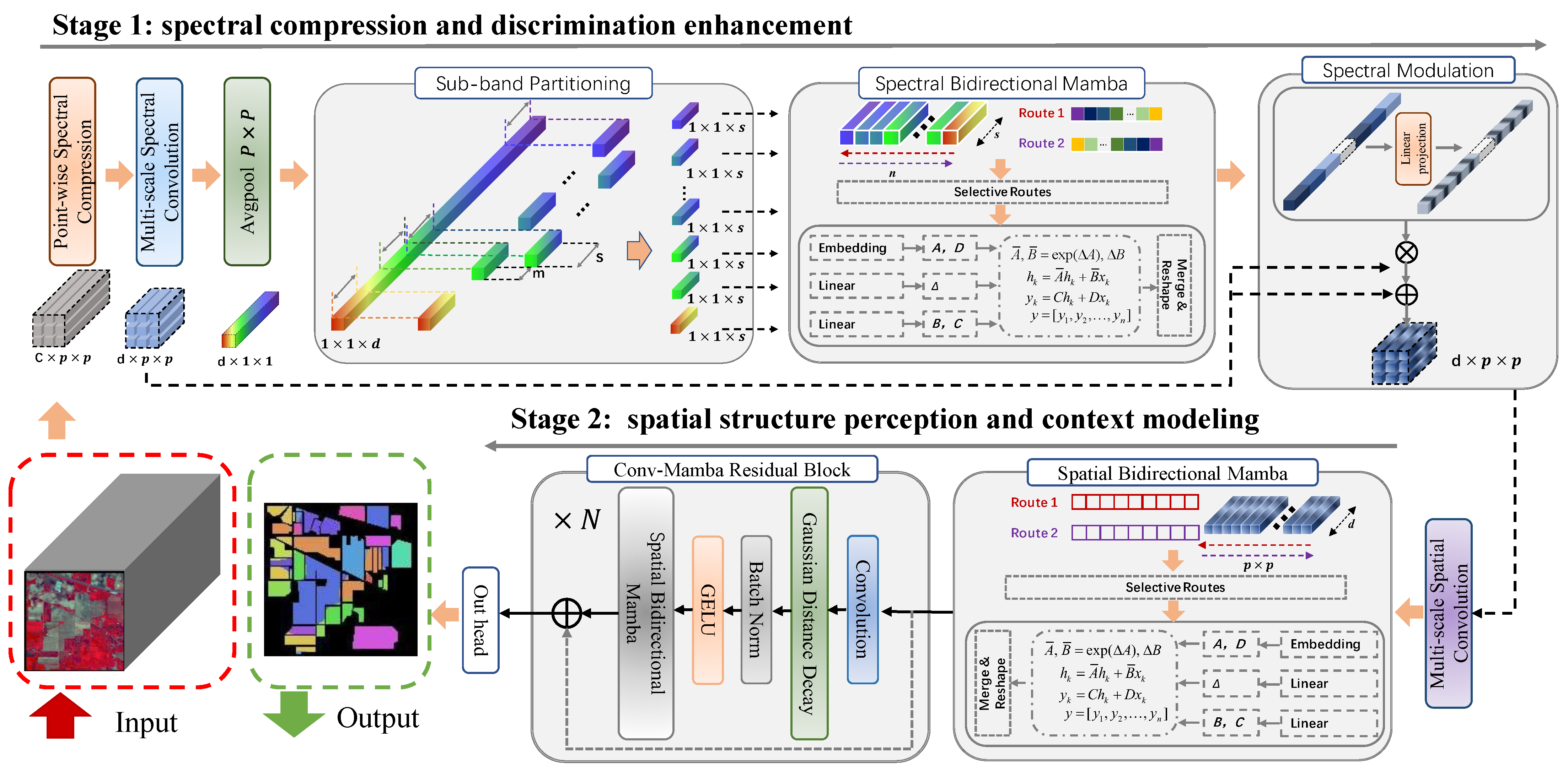
4.1. Overall Architecture

HG-Mamba is a hybrid bidirectional Mamba network developed to address challenges such as spectral redundancy, spatial heterogeneity, and unidirectional modeling in HSI classification. The framework employs a two-stage sequential pipeline (as illustrated in Figure 2). It integrates convolutional operations, geometry-aware filtering, and bidirectional state-space models (SSMs) to facilitate robust spectral–spatial feature learning. In Stage 1, termed spectral compression and discrimination enhancement, redundant spectral bands are suppressed while discriminative features are enhanced through multi-scale spectral convolutions and bidirectional SSMs. Stage 2, named spatial structure perception and context modeling, focuses on capturing geometry-aware spatial dependencies and long-range contextual relationships via a Gaussian Distance Decay (GDD) module and bidirectional spatial Mamba blocks.

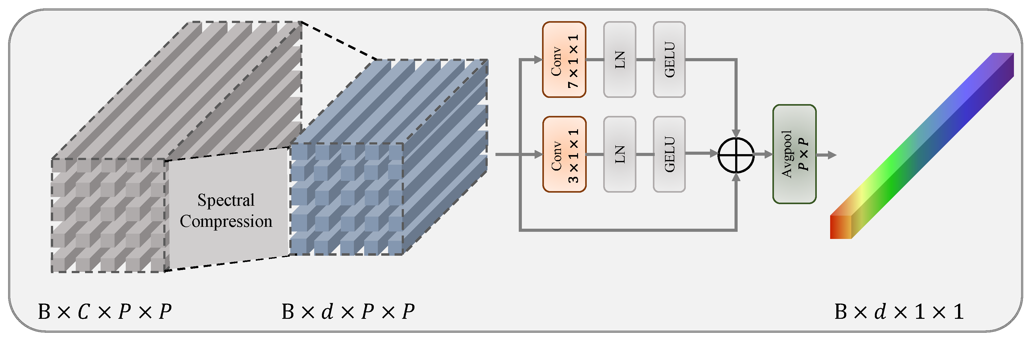
4.2. Spectral Compression and Discrimination Enhancement

The first stage of HG-Mamba aims to reduce spectral redundancy and enhance discriminative spectral features that are relevant to the classification task. Given an input hyperspectral image patch $\mathbf{X}\in {\mathbb{R}}^{B\times C\times P\times P}$, where C denotes the number of spectral bands and $P\times P$ is the spatial patch size, a point-wise $1\times 1$ convolution is first applied to compress the spectral dimension into a lower-dimensional embedding space of size d:

$${\mathbf{X}}_0=\varphi \left(\mathrm{BN}\left({\mathrm{Conv}}_{1\times 1}\left(\mathbf{X}\right)\right)\right)$$

(12)

where ${\mathbf{X}}_0\in {\mathbb{R}}^{B\times d\times P\times P}$, $\varphi$ denotes the GELU activation function, and $\mathrm{BN}(·)$ represents the batch normalization operation.

To enhance the extraction of localized spectral details, the feature map ${\mathbf{X}}_0$ is reshaped to ${\mathbb{R}}^{B\times H\times W\times d}$ and passed through two parallel spectral convolution branches. These branches apply 3D convolutions with kernel sizes of $3\times 1\times 1$ and $7\times 1\times 1$, respectively, to capture contextual spectral dependencies at different receptive fields:

$$\begin{array}{c}\hfill {\mathbf{S}}_3=\varphi \left(\mathrm{LN}\left({\mathrm{Conv}}_{3\times 1\times 1}\left({\mathbf{X}}_0\right)\right)\right)\end{array}$$

(13)

$$\begin{array}{c}\hfill {\mathbf{S}}_7=\varphi \left(\mathrm{LN}\left({\mathrm{Conv}}_{7\times 1\times 1}\left({\mathbf{X}}_0\right)\right)\right)\end{array}$$

(14)

where $\varphi$ denotes the GELU activation function, and $\mathrm{LN}(·)$ represents the layer normalization operation, as illustrated in Figure 3.

The outputs of both branches are fused with the original feature map by element-wise addition to obtain the enhanced spectral representation:

$$\mathbf{S}={\mathbf{S}}_3+{\mathbf{S}}_7+{\mathbf{X}}_0$$

(15)

Next, global average pooling is performed along the spatial dimensions to obtain a compressed spectral representation ${\mathbf{S}}_g\in {\mathbb{R}}^{B\times d\times 1\times 1}$. Then, the spectral dimension is partitioned into multiple overlapping sub-bands, where each sub-band has a width of s (i.e., spec_num) and a sliding stride of m (i.e., move_num). This results in a set of spectral sub-sequences ${\left\{{\mathbf{S}}^{\left(i\right)}\right\}}_{i=1}^n$, with each ${\mathbf{S}}^{\left(i\right)}\in {\mathbb{R}}^{B\times s}$. The above parameter configuration follows the sliding sub-band partitioning strategy proposed by Pan et al. [33]. Specifically, we set the sub-band width $s=12$ and the sliding stride $m=6$, corresponding to a coverage rate of $c=0.5$. A smaller s captures fine-grained details but may lose contextual information, while a larger s increases redundancy. A moderate window length balances local detail and global context. Similarly, a moderate coverage rate provides sufficient overlap between sub-bands to ensure robustness without incurring excessive computational cost. Based on the embedding dimension d, the number of sub-bands n is computed as:

$$n=⌊{\displaystyle \frac{d-s}{m}}⌋+1$$

(16)

To model inter-sub-band contextual dependencies, we introduce the Spectral Bidirectional Mamba (SeBM) module. Given the sequence of spectral sub-bands ${\left\{{\mathbf{S}}^{\left(i\right)}\right\}}_{i=1}^n$ generated earlier, SeBM performs bidirectional state-space modeling to capture global correlations among different sub-bands, thereby enhancing cross-band information integration. The entire process can be described as:

$${\mathbf{Z}}_s={\mathcal{M}}_{\mathrm{SeBM}}\left(\left\{{\mathbf{S}}^{\left(i\right)}\right\}\right)\in {\mathbb{R}}^{B\times n\times s}$$

(17)

Next, we flatten ${\mathbf{Z}}_s$ into ${\mathbb{R}}^{B\times (n·s)}$, and feed it into a fully connected layer with LayerNorm and GELU activation to obtain a compact global spectral descriptor:

$$\mathbf{z}=\varphi \left(\mathrm{LN}\left(\mathrm{FC}\left({\mathbf{Z}}_s\right)\right)\right)\in {\mathbb{R}}^{B\times d}$$

(18)

This descriptor is then reshaped to ${\mathbb{R}}^{B\times d\times 1\times 1}$, and used to modulate the original spectral features ${\mathbf{X}}_0$ through element-wise multiplication, forming a spectral attention mechanism:

$${\mathbf{X}}_1={\mathbf{X}}_0\odot \mathbf{z}$$

(19)

Such modulation enhances the response of spectrally informative components while suppressing noisy or redundant ones, thereby improving feature discriminability. The modulated features ${\mathbf{X}}_1$ are then forwarded into the spatial modeling stage as input.

4.3. Spatial Structure Perception and Context Modeling

This stage is dedicated to modeling spatial dependencies to enhance the extraction of local textures and global contextual semantics. This stage takes the spectrally modulated feature map from Stage 1, ${\mathbf{X}}_1\in {\mathbb{R}}^{B\times d\times P\times P}$, as input.

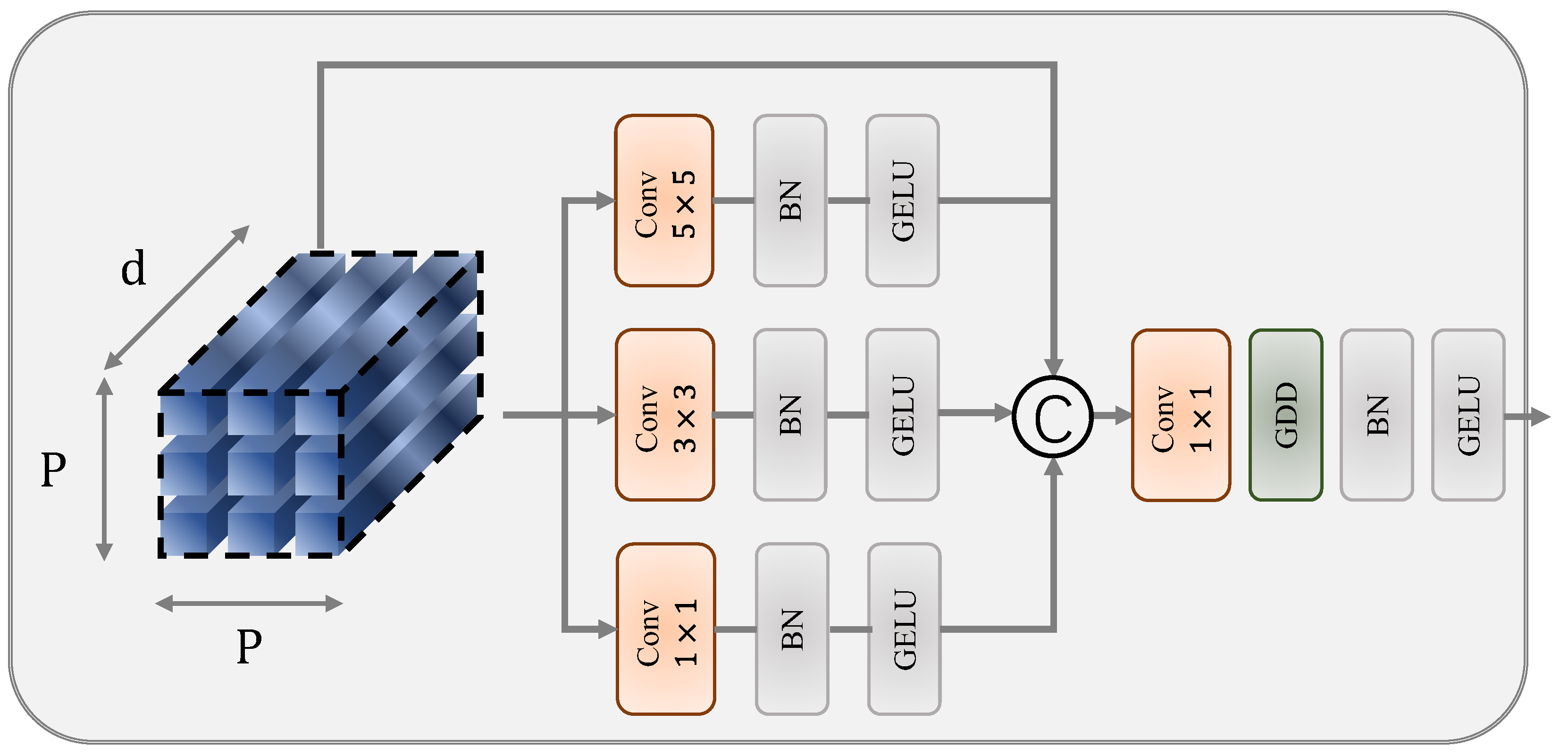
4.3.1. Multi-Scale Spatial Structure Extraction

To effectively capture multi-scale spatial structural information, we design a multi-branch convolutional feature extraction module to simultaneously model local texture details at different spatial scales. As illustrated in Figure 4, the input feature map ${\mathbf{X}}_1\in {\mathbb{R}}^{B\times d\times P\times P}$ is first passed through three parallel convolutional branches with varying receptive fields (i.e., kernel sizes of $1\times 1$, $3\times 3$, and $5\times 5$). The small kernel helps extract fine-grained edge and texture features, while the larger kernels enhance regional semantics. These three branches produce intermediate features ${\mathbf{F}}_1$, ${\mathbf{F}}_3$, and ${\mathbf{F}}_5\in {\mathbb{R}}^{B\times d\times P\times P}$, respectively. These are then concatenated with the original feature ${\mathbf{X}}_1$ along the channel dimension to construct a multi-scale fused representation ${\mathbf{F}}_{\mathrm{cat}}\in {\mathbb{R}}^{B\times 4d\times P\times P}$, with the concatenation operation defined as:

$${\mathbf{F}}_{\mathrm{cat}}=\mathrm{Concat}({\mathbf{X}}_1,{\mathbf{F}}_1,{\mathbf{F}}_3,{\mathbf{F}}_5)$$

(20)

4.3.2. Gaussian Distance Decay (GDD)

To incorporate geometry-awareness into spatial modeling, we design a Gaussian distance-weighted spatial filtering mechanism, referred to as Gaussian Distance Decay (GDD). The GDD module is embedded within the fusion operation to enhance spatial interactions with distance sensitivity.

This module employs a learnable geometry-aware convolution kernel to assign distance-based weights to different spatial locations, thereby emphasizing structurally salient regions while suppressing weakly correlated areas. The core idea is as follows. The importance of a pixel in spatial structures is not solely determined by its content features. It is also influenced by its geometric distance from the central position. To this end, we use a learnable Gaussian kernel to reweight spatial responses based on relative distances, enabling a geometry-sensitive filtering operation.

Specifically, GDD first constructs a 2D Euclidean distance grid $\mathbf{G}(i,j)$ of size $k\times k$, where each element represents the distance from pixel $(i,j)$ to the kernel center:

$$\mathbf{G}(i,j)=\sqrt{{(i-c)}^2+(j-c{)}^2}$$

(21)

where $c={\displaystyle \frac{k-1}{2}}$ denotes the coordinate of the kernel center. Based on this distance map, GDD constructs a learnable Gaussian weighting kernel as follows:

$$\mathbf{W}(i,j)={\displaystyle \frac{1}{Z}}exp\left(-{\displaystyle \frac{\mathbf{G}{(i,j)}^2}{2{\sigma }^2}}\right)$$

(22)

Here, $\sigma$ is a learnable smoothing parameter that controls the decay rate of spatial responses with respect to distance. Z is a normalization factor that ensures the sum of the kernel weights equals 1. To enable group-wise depthwise convolution, the Gaussian kernel is expanded to shape $[C,1,k,k]$, so that each channel uses an independent geometric filter.

After constructing the Gaussian kernel, we apply it in a depthwise convolutional manner to reweight spatial features. Let ${\mathbf{F}}_{\mathrm{cat}}\in {\mathbb{R}}^{B\times 4d\times P\times P}$ denote the concatenated multi-scale features obtained from the previous convolutional branches. These features are first compressed back to the original embedding dimension d via a $1\times 1$ convolution:

$${\mathbf{F}}_{\mathrm{proj}}={\mathrm{Conv}}_{1\times 1}\left({\mathbf{F}}_{\mathrm{cat}}\right)\in {\mathbb{R}}^{B\times d\times P\times P}$$

(23)

Then, the geometry-aware GDD filtering is applied to ${\mathbf{F}}_{\mathrm{proj}}$ as a channel-wise depthwise convolution:

$${\mathbf{F}}_{\mathrm{gdd}}=\mathrm{GDD}\left({\mathbf{F}}_{\mathrm{proj}}\right)\in {\mathbb{R}}^{B\times d\times P\times P}$$

(24)

Finally, the filtered feature ${\mathbf{F}}_{\mathrm{gdd}}$ is normalized and activated to obtain the fused spatial representation:

$${\mathbf{F}}_{\mathrm{fused}}=\varphi \left(\mathrm{BN}\left({\mathbf{F}}_{\mathrm{gdd}}\right)\right)\in {\mathbb{R}}^{B\times d\times P\times P}$$

(25)

Here, $\varphi (·)$ denotes the GELU activation function and $\mathrm{BN}(·)$ is batch normalization. This fusion process integrates multi-scale spatial features and enhances geometry-aware representation for subsequent contextual modeling.

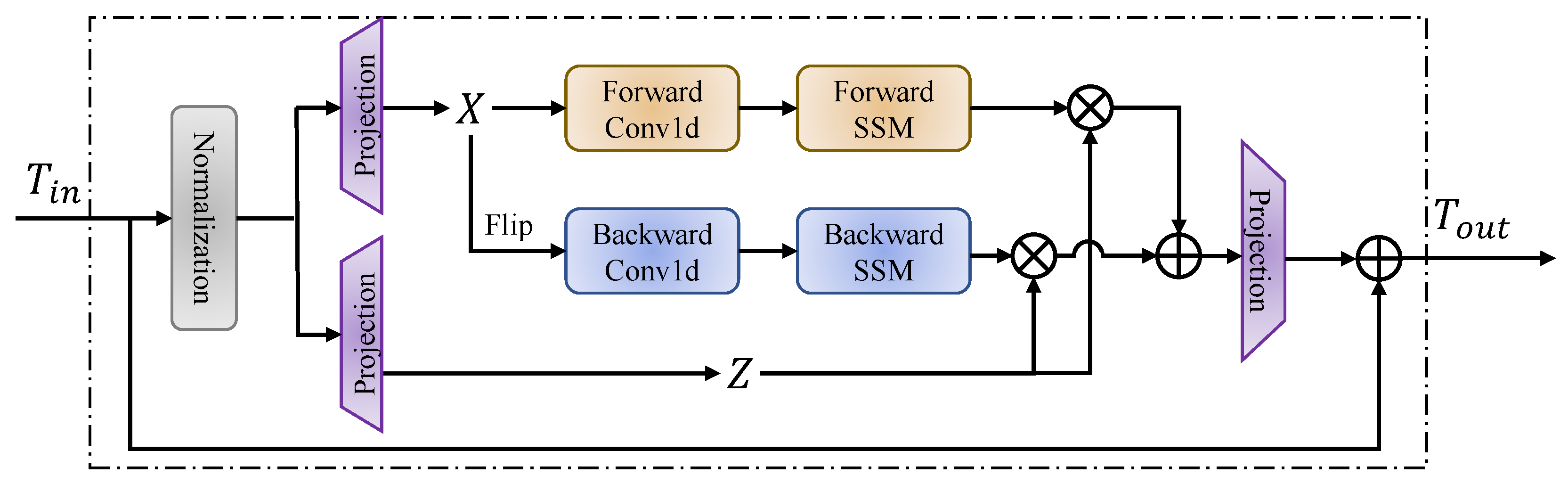
4.3.3. Hierarchical Refinement with Spatial Bidirectional Mamba

To further capture long-range spatial dependencies, we flatten the fused features ${\mathbf{F}}_{\mathrm{fused}}$ along spatial dimensions into a sequence $\mathbf{T}\in {\mathbb{R}}^{B\times (P·P)\times d}$, which is then fed into an SaBM module to enable bidirectional sequence modeling:

$${\mathbf{T}}^{\prime }={\mathcal{M}}_{\mathrm{SaBM}}\left(\mathbf{T}\right)\in {\mathbb{R}}^{B\times (P·P)\times d}$$

(26)

The output sequence is reshaped back to its original spatial format:

$${\mathbf{F}}_{\mathrm{ctx}}=\mathrm{Reshape}\left({\mathbf{T}}^{\prime }\right)\in {\mathbb{R}}^{B\times d\times P\times P}$$

(27)

To further refine the hierarchical spatial representations, the context-enhanced feature ${\mathbf{F}}_{\mathrm{ctx}}$ is passed through a stack of L Conv-Mamba residual blocks. In each block, local features are extracted using a convolutional layer followed by GDD, batch normalization, and GELU activation. These locally refined features are then passed into a SaBM module to capture long-range spatial dependencies. A residual connection integrates the Mamba-enhanced output with the input, forming the final representation ${\mathbf{X}}_2$ after N residual refinements.

The final output feature map ${\mathbf{X}}_2\in {\mathbb{R}}^{B\times d\times P\times P}$ is globally pooled and fed into a linear classifier to produce the final predictions. This process is formulated as:

$$\widehat{\mathbf{y}}=\mathrm{FC}\left(\mathrm{GAP}\left({\mathbf{X}}_2\right)\right)\in {\mathbb{R}}^{B\times N_c}$$

(28)

where $\mathrm{GAP}(·)$ denotes the global average pooling operation, $\mathrm{FC}(·)$ is a fully connected layer, $N_c$ is the number of target classes, and $\widehat{\mathbf{y}}$ represents the predicted class logits.

5. Experiments

5.1. Datasets and Setting

Datasets. Three HSI datasets are utilized in our experiments, including the Indian Pines scene, Houston2013, and WHU-Hi-LongKou (WHL) datasets.

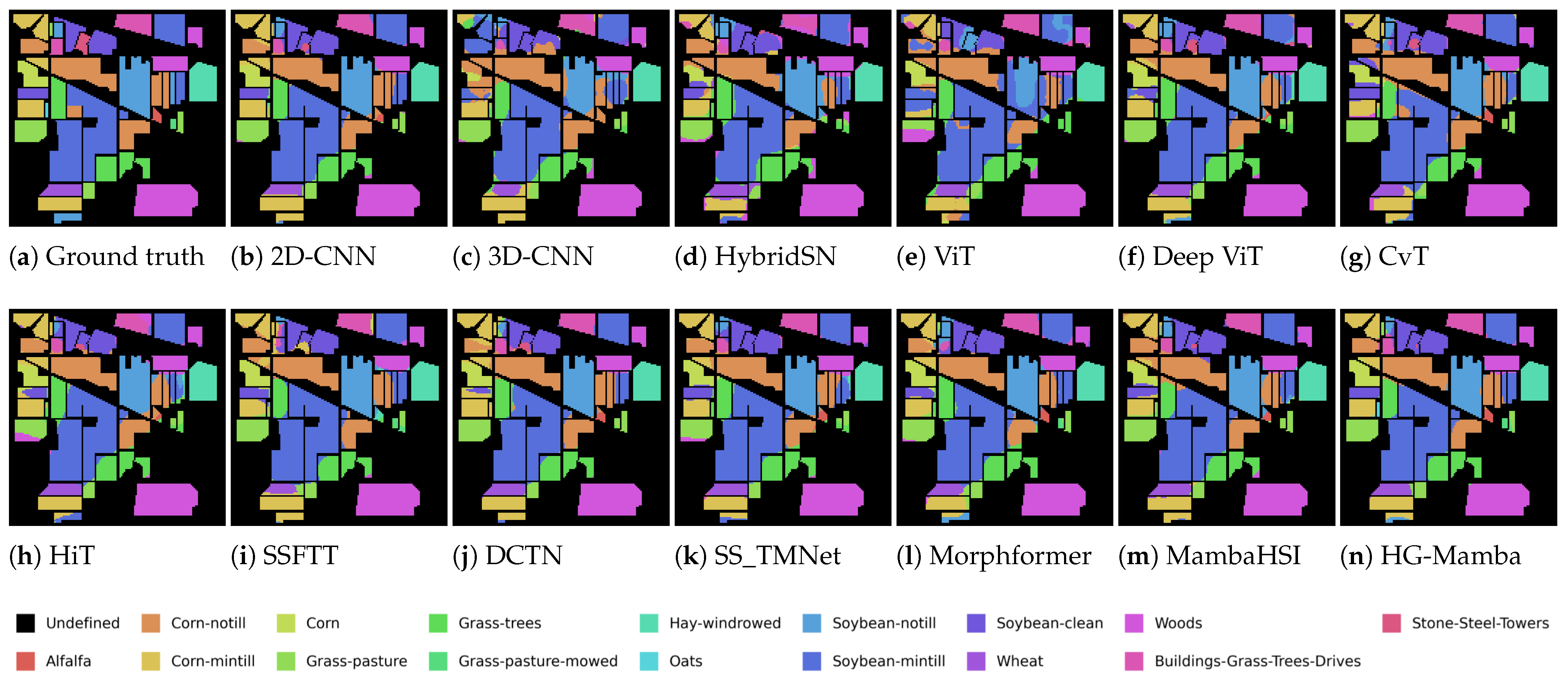
• Indian Pines Scene: This HSI dataset was acquired in 1992 by the Airborne Visible Imaging Spectrometer (AVIRIS) instrument over a mixed agricultural and forest area in Northwestern Indiana, USA. The original imagery comprised 220 spectral bands. After preprocessing that involved the removal of 20 noisy bands, 200 spectral bands were retained for analysis. The spatial dimensions of the image are 145 × 145 pixels. The scene includes 16 distinct land cover classes, encompassing a variety of agricultural and natural surface types. The complete set of classes is as follows: Alfalfa, Corn-notill, Corn-mintill, Corn, Grass-pasture, Grass-trees, Grass-pasture-mowed, Hay-windrowed, Oats, Soybean-notill, Soybean-mintill, Soybean-clean, Wheat, Woods, Buildings-Grass-Trees-Drives, and Stone-Steel-Towers.
  For the purpose of training and testing, a subset constituting 10% of the total labeled samples was allocated for model training, with the remaining 90% designated for performance evaluation.
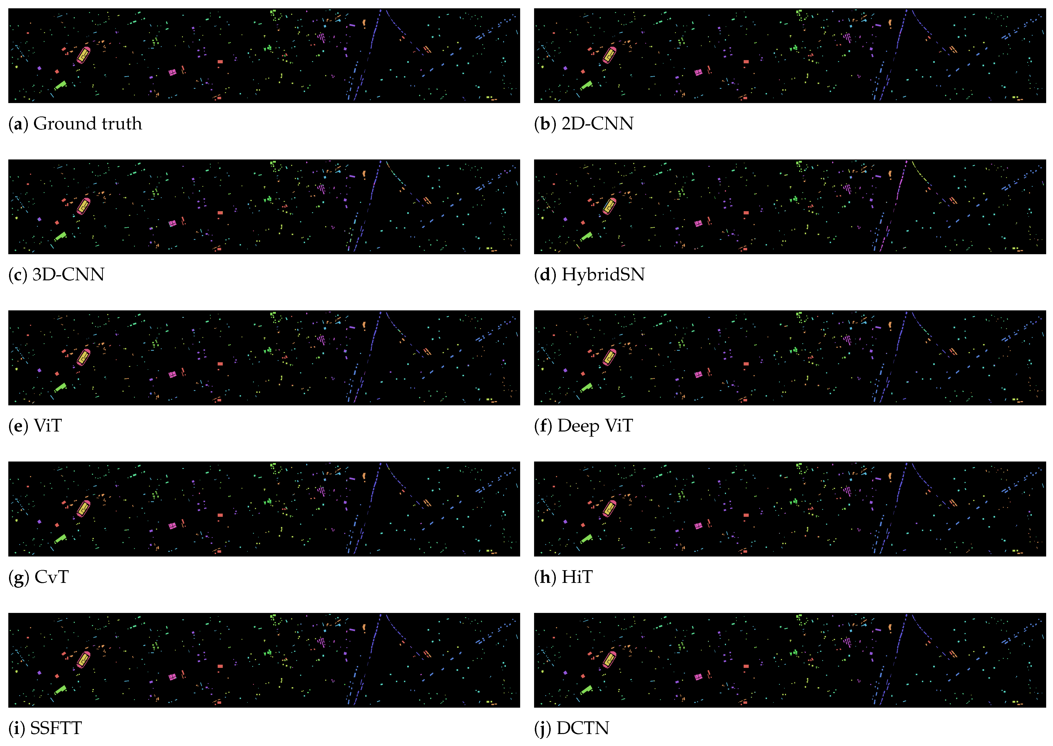
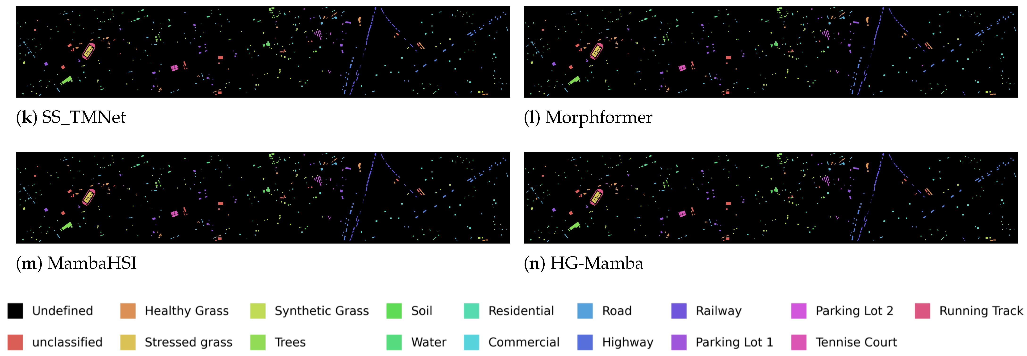
• Houston2013 Dataset: This dataset captures an urban scene covering the University of Houston and its vicinities in Texas, USA. The data was collected using the ITRES CASI-1500 sensor. The imagery provides spatial dimensions of 349 × 1905 pixels and contains 144 spectral band. Provided as a cloud-free image by the Geo-science and Remote Sensing Society (GRSS), it serves as a standard benchmark. The dataset is composed of a total of 15 labeled land cover classes. The complete set of classes includes: Grass-healthy, Grass-stressed, Grass-synthetic, Tree, Soil, Water, Residential, Commercial, Road, Highway, Railway, Parking Lot 1, Parking Lot 2, Tennis Court, and Running Track.
  In our experimental setup, 10% of the available samples were selected to form the training set, while the remaining samples constituted the test set.
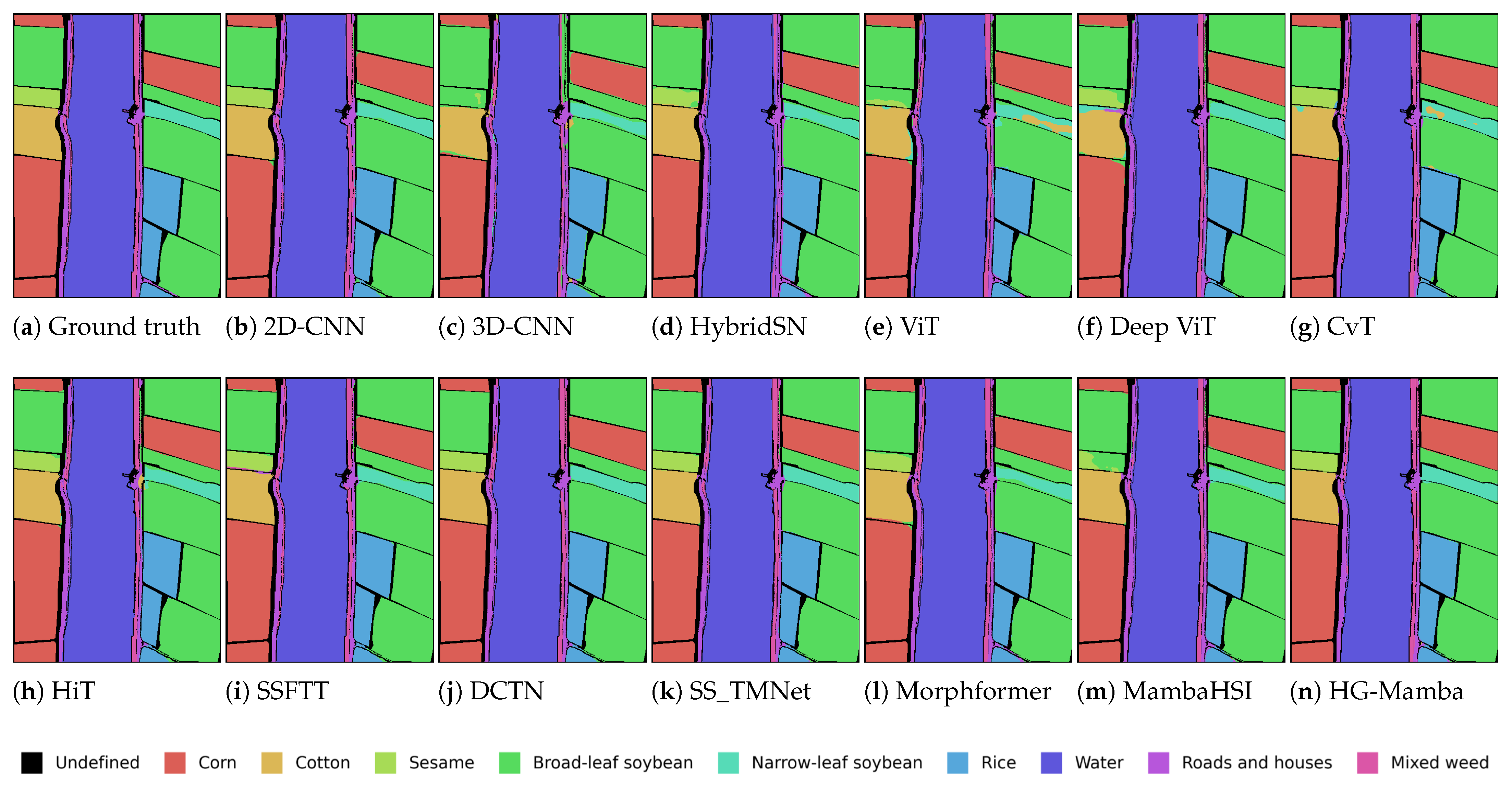
• WHU-Hi-LongKou (WHL) Dataset: Acquired on 17 July 2018, this dataset covers Longkou Town, Hubei province, China. Data collection was performed via a UAV platform (DJI Matrice 600 Pro) equipped with a Headwall Nano-Hyperspec imaging sensor featuring an 8 mm focal length. The UAV flew at an altitude of 500 m, resulting in imagery with a spatial resolution of 550 × 400 pixels. The spectral range of the sensor spans from 400 to 1000 nm, capturing data across 270 bands. The dataset comprises 204,542 labeled samples distributed among nine distinct land cover classes. The complete set of classes includes: Corn, Cotton, Sesame, Broad-leaf soybean, Narrow-leaf soybean, Rice, Water, Roads and houses, and Mixed weed.
  In this study, a small fraction, specifically 1%, of the labeled samples was utilized for training, with the predominant portion (99%) reserved for testing.

Evaluation Metrics. To quantify the performance of the classification methods, three standard metrics were employed: Overall Accuracy (OA), Average Accuracy (AA), and the Kappa Coefficient ($\kappa$).

Comparison Methods. We conducted comprehensive comparisons with state-of-the-art methods across different architectural paradigms: CNN-based (e.g., 2D-CNN [6], 3D-CNN [7], HybridSN [37]), Transformer-based (e.g., ViT [38], DeepViT [39], CvT [40], HiT [41], MorphFormer [13], SSTMNet [42], DCTN [32], and SSFTT [14]), and SSM-based (MambaHSI [17], ${\mathrm{S}}^2$Mamba [43]).

Setting. For the training process, 100 patches with spatial dimensions of 15 × 15 pixels were randomly cropped and utilized as input samples. The training procedure was executed for 100 iterations. All comparison methods and the proposed HG-Mamba model were implemented within the PyTorch 2.1.1 framework. The HG-Mamba model’s parameters were updated using the Adam optimizer. Furthermore, the learning rate was configured to 1 × 10⁻³, and the batch size was set at 100.

5.2. Results and Analysis

In this section, we provide a comprehensive analysis of the experimental results obtained from the Indian Pines, Houston2013, and WHU-Hi-LongKou (WHL) benchmark datasets, as presented in

Table 1. Comparisons with the state-of-the-art models on the Indian Pines Scene dataset (10% training samples).

Class	2D-CNN	3D-CNN	Hybridsn	ViT	Deep ViT	CvT	HiT	SSFTT	MorphFormer	SS_TMNet	DCTN	MambaHSI	S2Mamba	HG-Mamba
Alfalfa	92.82 ± 4.80	69.95 ± 17.92	18.85 ± 29.79	80.76 ± 5.74	81.65 ± 10.84	48.74 ± 15.97	14.63 ± 19.68	89.65 ± 6.91	82.13 ± 22.40	87.48 ± 8.15	72.29 ± 11.04	54.15 ± 14.91	10.73 ± 11.91	94.15 ± 4.39
Corn-notill	93.81 ± 1.97	88.61 ± 1.17	84.84 ± 11.22	94.29 ± 0.77	94.14 ± 1.06	91.40 ± 2.24	90.74 ± 0.89	94.11 ± 1.08	93.38 ± 2.14	88.56 ± 2.34	95.70 ± 1.57	89.07 ± 2.22	84.01 ± 3.29	92.61 ± 3.28
Corn-mintill	92.19 ± 1.77	86.74 ± 1.90	75.93 ± 18.40	93.63 ± 0.58	92.86 ± 1.30	85.23 ± 4.89	86.88 ± 1.90	90.13 ± 2.66	91.28 ± 3.66	76.50 ± 3.23	88.93 ± 1.40	89.10 ± 6.23	90.19 ± 4.64	97.32 ± 1.85
Corn	97.94 ± 1.50	93.92 ± 2.44	80.93 ± 17.01	99.62 ± 0.28	99.22 ± 1.22	92.32 ± 4.40	79.81 ± 11.13	94.90 ± 3.46	95.26 ± 4.04	82.19 ± 3.92	92.77 ± 2.77	91.60 ± 5.31	93.43 ± 6.32	97.70 ± 2.94
Grass-pasture	93.09 ± 3.32	93.44 ± 0.70	73.56 ± 16.43	92.00 ± 1.11	89.45 ± 2.91	88.40 ± 2.40	83.91 ± 9.24	93.08 ± 2.52	94.72 ± 1.55	81.71 ± 3.49	92.04 ± 1.28	87.38 ± 7.67	75.82 ± 20.84	95.54 ± 2.30
Grass-trees	95.65 ± 2.97	94.82 ± 0.67	75.90 ± 15.75	90.79 ± 1.41	90.74 ± 2.85	93.92 ± 1.02	94.06 ± 0.63	95.98 ± 1.29	95.47 ± 1.38	97.76 ± 0.92	98.64 ± 0.68	93.21 ± 2.30	91.54 ± 2.36	95.95 ± 5.36
Grass-pasture-mowed	7.94 ± 18.29	0.00 ± 0.00	0.00 ± 0.00	0.00 ± 0.00	0.00 ± 0.00	8.08 ± 22.04	0.00 ± 0.00	54.69 ± 35.84	71.56 ± 18.01	72.09 ± 16.30	73.76 ± 9.76	0.00 ± 0.00	0.00 ± 0.00	83.60 ± 28.65
Hay-windrowed	99.69 ± 0.55	98.87 ± 1.10	87.72 ± 13.09	99.77 ± 0.22	99.79 ± 0.17	99.31 ± 0.81	100.00 ± 0.00	98.77 ± 1.35	99.81 ± 0.39	94.39 ± 0.47	97.75 ± 0.95	99.79 ± 0.63	100.00 ± 0.00	100.00 ± 0.00
Oats	73.30 ± 29.09	0.00 ± 0.00	2.45 ± 5.09	4.29 ± 10.09	25.28 ± 27.21	8.49 ± 15.63	0.00 ± 0.00	54.34 ± 32.04	21.28 ± 30.14	68.66 ± 17.26	76.70 ± 15.73	0.00 ± 0.00	0.00 ± 0.00	90.00 ± 13.56
Soybean-notill	87.78 ± 1.60	83.25 ± 1.22	78.05 ± 9.87	89.90 ± 0.36	88.77 ± 1.22	84.38 ± 1.41	84.11 ± 0.27	87.11 ± 1.77	88.80 ± 3.58	87.19 ± 1.98	93.57 ± 1.21	80.54 ± 3.20	81.28 ± 2.00	82.15 ± 3.53
Soybean-mintill	96.26 ± 1.24	94.38 ± 0.51	91.41 ± 4.16	96.55 ± 0.12	96.65 ± 0.55	94.64 ± 0.63	97.06 ± 0.06	96.78 ± 0.82	96.27 ± 0.59	90.70 ± 1.63	95.46 ± 0.53	97.61 ± 1.33	97.59 ± 1.22	99.03 ± 0.40
Soybean-clean	91.80 ± 2.21	89.11 ± 1.71	78.53 ± 12.76	92.96 ± 1.34	93.57 ± 1.30	86.16 ± 5.24	91.20 ± 0.42	89.52 ± 3.35	87.66 ± 5.08	81.85 ± 3.97	94.68 ± 1.39	93.03 ± 4.38	94.51 ± 2.01	94.91 ± 1.81
Wheat	98.12 ± 1.32	86.71 ± 7.81	54.68 ± 33.43	96.73 ± 1.43	97.08 ± 1.64	89.64 ± 4.40	100.00 ± 0.00	95.00 ± 3.62	94.35 ± 4.88	97.18 ± 3.02	99.89 ± 0.18	94.38 ± 7.55	86.11 ± 6.01	92.38 ± 6.74
Woods	98.28 ± 2.42	97.81 ± 0.58	94.10 ± 5.22	98.27 ± 0.38	97.75 ± 0.75	98.39 ± 0.52	99.56 ± 0.17	98.67 ± 0.66	98.87 ± 0.31	96.21 ± 0.89	98.49 ± 0.40	99.58 ± 0.44	99.52 ± 0.25	98.88 ± 1.28
Buildings-Grass-Trees-Drives	97.82 ± 1.46	93.48 ± 2.25	73.19 ± 17.09	98.00 ± 0.60	98.25 ± 1.12	91.41 ± 3.60	86.17 ± 1.47	96.08 ± 2.76	96.06 ± 1.48	63.92 ± 3.78	77.76 ± 1.60	86.48 ± 9.27	87.67 ± 5.33	95.19 ± 2.69
Stone-Steel-Towers	52.74 ± 21.39	46.87 ± 17.62	41.04 ± 32.91	53.30 ± 17.49	63.78 ± 21.77	67.35 ± 23.50	8.33 ± 22.82	39.20 ± 32.30	25.11 ± 33.47	87.73 ± 3.15	96.80 ± 1.98	29.05 ± 25.48	0.00 ± 0.00	43.93 ± 23.09
OA (%)	94.48 ± 1.41	91.48 ± 0.52	83.10 ± 10.19	94.50 ± 0.30	94.28 ± 0.43	91.41 ± 0.93	91.02 ± 0.95	94.09 ± 0.97	94.03 ± 0.90	84.67 ± 1.25	92.85 ± 0.41	91.50 ± 0.67	89.84 ± 1.26	94.91 ± 0.51
AA (%)	83.81 ± 3.38	73.92 ± 2.12	62.87 ± 12.02	78.40 ± 1.18	79.90 ± 2.11	77.31 ± 2.41	69.78 ± 4.52	84.54 ± 3.91	82.75 ± 2.85	85.56 ± 4.91	86.55 ± 3.55	74.06 ± 1.50	68.27 ± 1.83	90.83 ± 2.84
$\kappa$ (%)	93.69 ± 1.61	90.25 ± 0.59	80.70 ± 11.52	93.71 ± 0.35	93.46 ± 0.49	90.20 ± 1.06	89.72 ± 1.07	93.25 ± 1.10	93.18 ± 1.03	82.66 ± 1.41	91.87 ± 0.47	90.28 ± 0.77	88.36 ± 1.45	94.18 ± 0.59

,

Table 2. Comparisons with the state-of-the-art models on the Houston2013 dataset (10% training samples).

Class	2D-CNN	3D-CNN	HybridSN	ViT	Deep ViT	CvT	HiT	SSFTT	Morphformer	SS_TMNet	DCTN	MambaHSI	S2Mamba	HG-Mamba
Healthy Grass	95.21 ± 1.66	91.06 ± 3.44	90.76 ± 1.88	87.43 ± 3.25	91.33 ± 2.17	87.30 ± 10.73	94.49 ± 0.52	96.42 ± 1.16	85.97 ± 8.75	97.60 ± 0.64	98.86 ± 0.50	94.08 ± 2.29	93.14 ± 1.48	96.47 ± 0.85
Stressed grass	95.51 ± 1.72	88.85 ± 6.46	86.26 ± 8.27	80.16 ± 5.76	83.59 ± 2.71	90.21 ± 4.40	91.22 ± 2.10	97.16 ± 1.42	88.97 ± 5.58	98.44 ± 0.56	99.33 ± 0.22	97.40 ± 1.29	97.50 ± 0.94	97.96 ± 1.47
Synthetic GrassTrees	99.24 ± 0.45	97.36 ± 3.06	95.85 ± 3.67	97.95 ± 0.85	98.64 ± 0.56	97.70 ± 2.80	98.97 ± 0.29	99.30 ± 0.58	91.37 ± 13.84	99.50 ± 0.23	99.74 ± 0.29	94.95 ± 2.05	95.27 ± 2.07	98.24 ± 1.13
Trees	94.72 ± 2.18	88.28 ± 4.52	79.71 ± 7.46	81.31 ± 6.65	83.87 ± 4.62	89.45 ± 3.27	89.26 ± 1.20	97.68 ± 0.90	90.96 ± 4.95	97.26 ± 0.96	99.21 ± 0.41	97.17 ± 0.87	92.68 ± 3.47	99.10 ± 0.87
Soil	99.81 ± 0.17	95.72 ± 3.71	96.41 ± 3.83	97.80 ± 1.25	98.62 ± 1.51	99.17 ± 0.67	99.53 ± 0.24	99.43 ± 0.63	97.96 ± 2.17	98.19 ± 0.33	98.65 ± 0.12	99.50 ± 0.56	99.87 ± 0.13	99.86 ± 0.43
Water	94.05 ± 0.97	86.16 ± 1.92	91.69 ± 3.12	86.50 ± 1.79	87.48 ± 2.36	93.58 ± 2.23	86.87 ± 0.82	93.61 ± 3.07	90.85 ± 4.25	93.67 ± 2.33	98.75 ± 1.07	84.38 ± 4.04	80.75 ± 4.77	89.04 ± 5.59
Residential	96.82 ± 1.02	83.00 ± 6.98	78.74 ± 17.12	87.38 ± 1.99	87.28 ± 2.68	92.51 ± 3.82	91.87 ± 0.83	97.52 ± 0.80	85.78 ± 24.73	94.54 ± 1.03	98.20 ± 0.45	97.00 ± 1.69	88.33 ± 5.12	98.35 ± 0.76
Commercial	97.62 ± 1.51	89.55 ± 1.61	93.01 ± 2.65	90.55 ± 3.34	94.05 ± 1.95	94.16 ± 3.55	96.41 ± 0.64	97.88 ± 1.24	90.76 ± 9.56	95.74 ± 1.35	98.22 ± 0.69	93.78 ± 1.64	95.32 ± 1.98	97.69 ± 1.29
Road	95.42 ± 1.51	85.03 ± 3.38	73.95 ± 14.36	86.62 ± 1.57	87.98 ± 1.78	87.78 ± 2.93	89.78 ± 0.99	96.70 ± 1.56	87.54 ± 7.99	94.29 ± 1.32	97.66 ± 0.56	92.94 ± 1.74	88.00 ± 3.06	98.97 ± 0.81
Highway	99.09 ± 1.57	91.67 ± 6.54	91.92 ± 7.92	96.43 ± 3.22	95.01 ± 3.44	97.50 ± 1.56	97.93 ± 0.51	99.78 ± 0.38	93.89 ± 9.76	96.91 ± 0.81	98.89 ± 0.49	99.27 ± 1.03	99.97 ± 0.08	99.98 ± 0.05
Railway	99.58 ± 0.46	81.57 ± 5.87	85.29 ± 7.92	93.86 ± 2.51	93.32 ± 4.12	94.73 ± 3.22	99.37 ± 0.45	99.76 ± 0.44	91.69 ± 16.26	94.94 ± 0.72	98.51 ± 0.33	98.79 ± 1.16	97.41 ± 1.50	99.39 ± 1.05
Parking Lot 1	97.88 ± 1.83	94.30 ± 1.81	95.79 ± 2.71	91.42 ± 4.91	93.49 ± 3.96	95.83 ± 3.47	98.68 ± 0.21	98.70 ± 1.24	88.63 ± 13.89	96.50 ± 1.00	98.96 ± 0.22	95.81 ± 1.75	97.49 ± 0.92	97.32 ± 1.59
Parking Lot 2	97.55 ± 2.44	81.89 ± 6.24	86.51 ± 8.08	91.84 ± 1.55	89.01 ± 4.03	95.80 ± 2.87	95.93 ± 1.53	98.54 ± 1.23	92.25 ± 6.66	93.42 ± 1.61	97.68 ± 1.01	95.85 ± 2.44	96.23 ± 2.16	98.86 ± 1.41
Tennise Court	99.98 ± 0.07	98.60 ± 0.97	92.98 ± 6.16	99.20 ± 0.85	98.43 ± 2.66	97.96 ± 3.28	99.99 ± 0.04	99.67 ± 0.47	99.04 ± 1.46	99.88 ± 0.19	100.00 ± 0.00	99.97 ± 0.08	100.00 ± 0.00	100.00 ± 0.00
Running Track	97.87 ± 1.71	94.77 ± 5.41	91.48 ± 5.60	96.93 ± 1.89	98.14 ± 0.72	96.65 ± 3.12	98.39 ± 0.33	98.95 ± 0.71	93.32 ± 7.49	98.98 ± 0.58	99.24 ± 0.88	99.21 ± 1.04	100.00 ± 0.00	99.83 ± 0.40
OA (%)	97.32 ± 0.48	89.54 ± 3.21	88.19 ± 4.75	90.27 ± 1.69	91.58 ± 1.50	93.52 ± 1.88	95.20 ± 0.33	98.15 ± 0.53	90.98 ± 7.71	96.22 ± 0.35	98.31 ± 0.16	96.33 ± 0.38	94.98 ± 0.55	98.41 ± 0.26
AA (%)	97.03 ± 0.37	89.74 ± 2.87	88.97 ± 4.09	90.45 ± 1.42	91.38 ± 1.43	93.74 ± 1.95	94.80 ± 0.32	97.81 ± 0.59	90.99 ± 7.46	95.15 ± 0.45	97.32 ± 0.36	96.01 ± 0.44	94.80 ± 0.59	98.07 ± 0.34
$\kappa$ (%)	97.10 ± 0.51	88.70 ± 3.47	87.24 ± 5.13	89.48 ± 1.83	90.89 ± 1.62	92.99 ± 2.04	94.81 ± 0.35	98.00 ± 0.58	90.24 ± 8.36	95.92 ± 0.38	98.17 ± 0.17	96.03 ± 0.41	94.57 ± 0.60	98.28 ± 0.28

and

Table 3. Comparisons with the state-of-the-art models on the WHL dataset (1% training samples).

Class	2D-CNN	3D-CNN	HybridSN	ViT	Deep ViT	CvT	HiT	SSFTT	Morphformer	SS_TMNet	DCTN	MambaHSI	S2Mamba	HG-Mamba
Corn	99.87 ± 0.03	99.34 ± 0.40	99.34 ± 0.58	99.33 ± 0.13	99.66 ± 0.08	99.83 ± 0.07	99.77 ± 0.04	99.71 ± 0.23	99.70 ± 0.28	99.86 ± 0.11	99.99 ± 0.01	99.43 ± 0.25	99.73 ± 0.19	99.87 ± 0.12
Cotton	99.72 ± 0.09	96.30 ± 1.24	97.55 ± 3.18	83.45 ± 0.89	96.41 ± 1.60	99.39 ± 0.23	97.74 ± 0.69	99.69 ± 0.25	98.18 ± 1.74	98.55 ± 1.50	99.98 ± 0.01	98.12 ± 1.90	99.56 ± 0.39	98.86 ± 0.91
Sesame	94.97 ± 1.27	55.88 ± 29.79	81.52 ± 14.54	51.31 ± 21.70	88.79 ± 4.29	97.91 ± 0.71	91.44 ± 1.50	92.35 ± 5.03	94.05 ± 5.56	95.42 ± 4.00	98.80 ± 0.68	69.48 ± 24.88	97.66 ± 1.66	98.90 ± 1.34
Broad-leaf soybean	99.12 ± 0.08	96.24 ± 0.89	98.22 ± 0.64	96.51 ± 0.67	98.52 ± 0.22	99.49 ± 0.09	98.71 ± 0.21	99.69 ± 0.16	99.51 ± 0.41	99.79 ± 0.10	99.95 ± 0.02	99.73 ± 0.09	99.89 ± 0.09	99.86 ± 0.09
Narrow-leaf soybean	95.42 ± 0.71	87.80 ± 2.44	81.06 ± 10.19	42.38 ± 7.08	89.80 ± 2.31	97.10 ± 1.00	95.35 ± 1.41	91.00 ± 4.09	88.15 ± 8.32	91.07 ± 4.08	94.13 ± 1.47	89.56 ± 3.82	94.16 ± 1.46	96.56 ± 1.61
Rice	98.57 ± 0.19	98.11 ± 0.66	97.28 ± 0.91	98.54 ± 0.40	98.87 ± 0.16	98.80 ± 0.11	99.26 ± 0.05	99.06 ± 0.66	98.77 ± 1.59	99.23 ± 0.25	99.18 ± 0.18	98.13 ± 0.52	99.24 ± 0.31	99.09 ± 0.42
Water	99.74 ± 0.04	99.51 ± 0.22	97.11 ± 0.53	99.28 ± 0.11	99.39 ± 0.18	99.70 ± 0.12	99.45 ± 0.04	99.95 ± 0.05	99.97 ± 0.01	99.98 ± 0.01	100.00 ± 0.00	99.99 ± 0.01	99.99 ± 0.00	99.81 ± 0.38
Roads and houses	85.56 ± 0.78	82.84 ± 2.22	78.60 ± 7.09	80.96 ± 2.04	83.05 ± 1.42	84.75 ± 0.96	87.96 ± 0.74	85.45 ± 5.91	89.66 ± 4.22	88.66 ± 3.04	80.26 ± 4.53	89.38 ± 3.52	85.76 ± 5.08	80.02 ± 6.18
Mixed weed	78.58 ± 2.04	79.05 ± 2.99	37.10 ± 12.86	77.37 ± 2.01	74.30 ± 2.89	79.17 ± 2.84	80.65 ± 1.01	84.71 ± 9.52	77.91 ± 7.96	78.67 ± 8.08	77.96 ± 4.87	74.92 ± 5.50	76.94 ± 3.02	87.52 ± 6.65
OA (%)	98.35 ± 0.09	96.60 ± 0.63	95.77 ± 0.80	95.28 ± 0.48	97.55 ± 0.17	98.50 ± 0.12	98.18 ± 0.11	98.58 ± 0.37	98.39 ± 0.38	98.61 ± 0.26	98.54 ± 0.14	97.96 ± 0.44	98.61 ± 0.15	98.67 ± 0.29
AA (%)	93.24 ± 0.46	84.58 ± 3.95	82.29 ± 3.59	77.94 ± 3.08	90.01 ± 1.04	94.34 ± 0.58	92.43 ± 0.53	94.62 ± 1.24	93.99 ± 1.76	94.58 ± 1.04	94.47 ± 0.57	90.97 ± 3.22	94.77 ± 0.51	95.61 ± 0.99
$\kappa$ (%)	97.82 ± 0.13	95.49 ± 0.85	94.38 ± 1.07	93.74 ± 0.65	96.76 ± 0.23	98.03 ± 0.16	97.60 ± 0.15	98.13 ± 0.49	97.88 ± 0.50	98.17 ± 0.35	98.08 ± 0.18	97.30 ± 0.59	98.17 ± 0.19	98.25 ± 0.38

. Our analysis focuses on evaluating the overall performance of the proposed HG-Mamba against state-of-the-art comparison methods from CNN-based, Transformer-based, and SSM-based categories, as well as examining per-class accuracies and model robustness.

As shown in Table 1, Table 2 and Table 3, the proposed HG-Mamba consistently achieves the highest Overall Accuracy (OA), Average Accuracy (AA), and Kappa Coefficient ($\kappa$) across all three benchmark datasets. On the Indian Pines dataset (10% training samples, Table 1), HG-Mamba achieves an OA of 94.91%, an AA of 90.83%, and a $\kappa$ of 94.18%, outperforming all comparison methods in terms of overall and average accuracy. Similarly, for the Houston2013 dataset (Table 2), HG-Mamba leads with an OA of 98.41%, AA of 98.07%, and $\kappa$ of 98.28%. The performance gains are particularly significant on the challenging WHL dataset, which uses only 1% of training samples (Table 3). Here, HG-Mamba demonstrates superior capability in learning from extremely limited data, achieving an OA of 98.67%, AA of 95.61%, and $\kappa$ of 98.25%. These results strongly validate the effectiveness of the proposed HG-Mamba framework.

Comparing HG-Mamba with methods from different architectural paradigms reveals the advantages of our hybrid design. CNN-based methods (2D-CNN, 3D-CNN, HybridSN) generally show lower overall accuracies compared to Transformer and SSM-based methods, highlighting their limitation in capturing global context. Transformer-based methods, leveraging self-attention for long-range dependencies, generally perform well, with recent architectures like DCTN and SSFTT serving as strong baselines. However, HG-Mamba still surpasses these methods, suggesting that our combination of convolutional local feature extraction with efficient SSM-based global modeling is more effective for HSI classification. The SSM-based MambaHSI, while efficient, is consistently outperformed by HG-Mamba, indicating that the bidirectional modeling and geometry-aware components in our architecture contribute significantly beyond a basic spatial–spectral Mamba model.

Furthermore, we analyze the per-class classification accuracies to assess the model’s performance on individual land cover categories, particularly those with limited training samples. As seen in Table 1, classes like ‘Grass-pasture-mowed’ and ‘Oats’ have very few labeled samples, leading to significantly lower accuracies and high standard deviations for many methods (some even achieving 0% accuracy). HG-Mamba demonstrates remarkably better performance on these challenging classes (e.g., 83.60% for ’Grass-pasture-mowed’, 90.00% for ’Oats’) compared to most baselines, indicating its robustness and ability to handle class imbalance and learn discriminative features even from scarce examples. This robustness is also reflected in the consistently lower standard deviations of OA, AA, and $\kappa$ for HG-Mamba across all datasets, suggesting higher stability in performance compared to several comparison methods.

The superior performance of HG-Mamba, corroborated by the visually clean and highly faithful classification maps (Figure 5, Figure 6 and Figure 7), can be attributed to the synergistic integration of its key components, which effectively combine local details and global representations. Specifically, the spectral compression and Spectral Bidirectional Mamba efficiently handle high spectral dimensionality and capture long-range spectral dependencies, enhancing discriminability. The multi-scale spatial convolutions extract hierarchical local features, while the GDD module accurately models spatial heterogeneity and boundary regions. Furthermore, the Spatial Bidirectional Mamba and Conv-Mamba residual blocks effectively capture global spatial context and refine spatial representations with linear complexity, overcoming limitations of unidirectional SSMs and computationally expensive attention mechanisms. In contrast, the classification maps produced by most comparison methods exhibit significant noise levels (Figure 5, Figure 6 and Figure 7), a finding consistent with the quantitative results (Table 1, Table 2 and Table 3). This can be explained by the fact that CNNs primarily focus on local features and overlook global representations, while Transformer models, despite their ability to model global features, typically suffer from high computational complexity. Although SSM-based models (like MambaHSI) offer an efficient alternative for long-range dependencies, they may lack proficiency in handling complex spatial details and boundaries. These limitations highlight that simply relying on a single architecture or limited fusion mechanisms may be insufficient for generating high-quality classification maps. Therefore, the ability to effectively and efficiently balance the extraction of local details and global contextual modeling is crucial, which is precisely the advantage of HG-Mamba’s hybrid architecture, clearly demonstrated in both its state-of-the-art performance and the smoother, more ground-truth-faithful classification maps it generates.

We also conducted a t-SNE visualization comparative analysis of the proposed HG-Mamba and five comparison methods, including CNN-based (e.g., 2D-CNN and 3D-CNN), Transformer-based (e.g., SSFTT and MorphFormer), and SSM-based (e.g., MambaHSI). The visualization results of different methods on the Indian Pines dataset are shown in Figure 8. According to Figure 8, we find that HG-Mamba can reduce inter-class confusion and enhance intra-class clustering, which is mainly due to HG-Mamba’s powerful feature learning ability; its hybrid convolutional–state-space model (Conv-SSM) structure effectively integrating local details and global representations, capturing more discriminative spatial–spectral features.

5.3. Comparison of Computational Complexity

Table 4. Comparison of computational complexity and performance.

Method	FLOPs (G)	Param (MB)	Training Time (s)	Testing Time (s)	OA (%)	AA (%)	$\mathit{\kappa }$ (%)
2D-CNN	0.77	1.71	30.13	1.28	94.48 ± 1.41	93.81 ± 3.38	93.69 ± 1.61
3D-CNN	1.35	1.45	81.48	2.56	91.48 ± 0.52	73.92 ± 2.12	90.25 ± 0.50
Deep ViT	13.69	52.75	142.50	3.69	94.28 ± 0.43	79.90 ± 2.11	93.46 ± 0.49
HiT	2.20	27.22	534.29	8.06	91.02 ± 0.95	69.78 ± 4.52	89.72 ± 1.07
MambaHSI	0.006	0.02	174.55	6.98	91.50 ± 0.67	74.06 ± 1.50	90.28 ± 0.77
HG-Mamba	0.57	1.30	248.20	8.88	94.91 ± 0.51	90.83 ± 2.84	94.18 ± 0.59

presents a comparison of the computational complexity (FLOPs and parameters), runtime (training and testing time), and classification performance of the proposed HG-Mamba and five representative comparison methods on the Indian Pines dataset.

As shown in Table 4, HG-Mamba achieves state-of-the-art classification accuracy in terms of OA, AA, and $\kappa$. Importantly, compared to Transformer-based methods such as Deep ViT (52.75 MB, 13.69 G) and HiT (27.22 MB, 2.20 G), HG-Mamba has significantly lower parameters (1.30 MB) and FLOPs (0.57 G), which is consistent with the theoretical efficiency advantages of SSMs. Compared to CNN-based methods (2D-CNN, 3D-CNN), HG-Mamba has competitive or slightly lower parameters, although its FLOPs are in a similar range to 2D-CNN but lower than 3D-CNN. While 2D-CNN and 3D-CNN offer faster training and testing times, HG-Mamba provides higher accuracy, especially in terms of AA. MambaHSI stands out with its extremely low FLOPs (0.006 G) and parameters (0.02 MB), demonstrating the significant advantages of SSMs in terms of model size and theoretical computation. However, HG-Mamba achieves significantly higher classification accuracy than MambaHSI, indicating that its hybrid architecture and specific components make important contributions to improving performance, despite the computational cost being slightly higher than MambaHSI itself. The training and testing times for HG-Mamba are moderate, faster than HiT but slower than CNNs and Deep ViT. This suggests a certain trade-off between speed and accuracy. Overall, the results show that HG-Mamba achieves an excellent balance between computational efficiency and classification performance, realizing state-of-the-art accuracy with a favorable complexity profile (especially in terms of model size and theoretical operations).

6. Ablation Studies

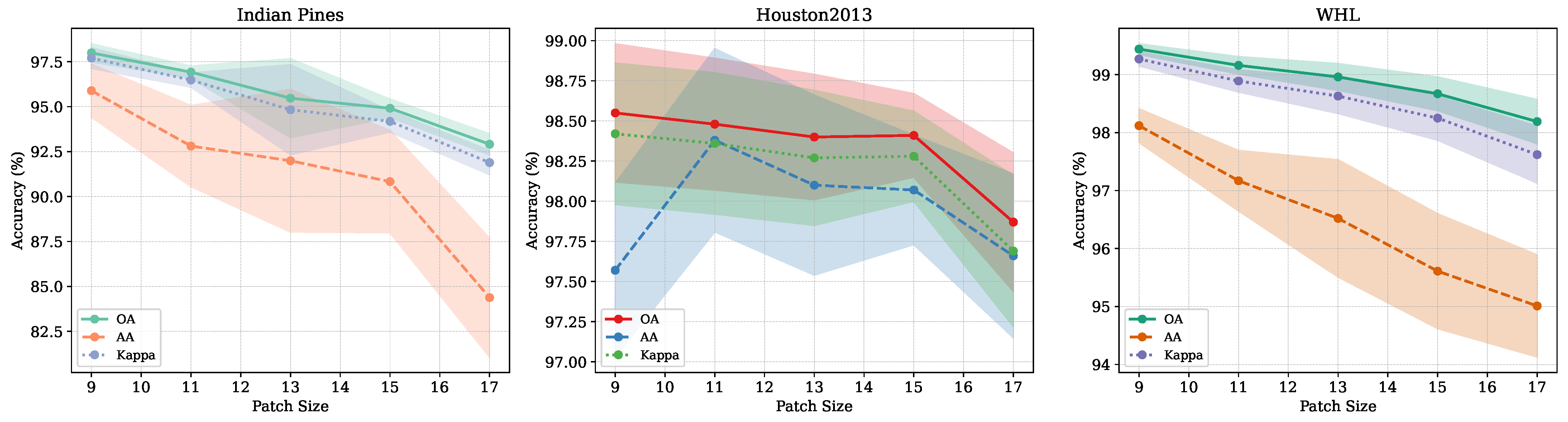
6.1. Patch Size Sensitivity Analysis

Figure 9 illustrates the sensitivity of HG-Mamba’s classification performance (OA, AA, $\kappa$) to varying patch sizes ($9\times 9$ to $17\times 17$) across three datasets. The optimal patch size is dataset-dependent, reflecting their distinct spatial characteristics. For Indian Pines (Figure 9, left), smaller patches yield better results, with performance decreasing as size increases. In contrast, Houston2013 (Figure 9, middle) and WHL (Figure 9, right) show performance peaking at moderate patch sizes (around 13 and 11, respectively). Across all datasets, performance consistently degrades with excessively large patches, suggesting that overly wide spatial context introduces noise. This highlights the importance of empirically selecting the appropriate patch size for optimal performance based on dataset characteristics.

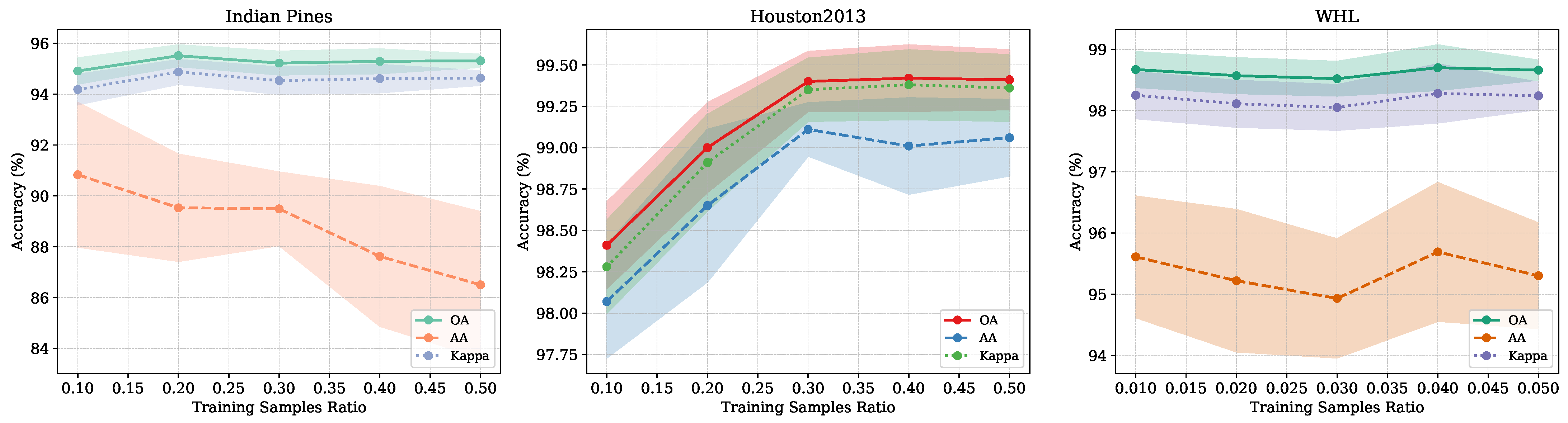
6.2. Training Sample Ratio Sensitivity Analysis

Figure 10 illustrates the classification performance (OA, AA, and $\kappa$) of HG-Mamba as the training sample ratio increases. As expected, performance generally improves with increased training data, but the rate of improvement and saturation point vary by dataset. For Indian Pines (Figure 10, left), OA and $\kappa$ show improvement, but AA exhibits a counter-intuitive trend, decreasing as the training ratio increases. This behavior in AA may be attributed to the severe class imbalance in the Indian Pines dataset; while the model learns better on more abundant classes with increased data, its performance on certain difficult or extremely sparse classes might not improve proportionally or could even slightly decrease relative to its overall learning focus, thus affecting the average per-class accuracy.

For Houston2013 (Figure 10, middle), all metrics show an initial sharp upward trend, followed by relatively quick saturation. On the challenging WHL dataset (Figure 10, right), the proposed model also shows some improvement, which highlights the model’s data efficiency.

6.3. Ablation Study of Different Modules

To analyze the contribution of each proposed module to the overall performance of HG-Mamba, we conducted an ablation study.

Table 5. Study of module contribution via ablation analysis.

Module Removed	OA (%)		AA (%)		$\mathit{\kappa }$ (%)
	Val ± Std	$\mathrm{\Delta }$	Val ± Std	$\mathrm{\Delta }$	Val ± Std	$\mathrm{\Delta }$
Stage 1	93.92 ± 0.48	(0.99↓)	85.87 ± 3.42	(4.96↓)	93.05 ± 0.55	(1.13↓)
Stage 2	92.98 ± 0.54	(1.93↓)	81.46 ± 2.83	(9.37↓)	91.98 ± 0.63	(2.20↓)
Spectral Bidirectional Mamba	94.53 ± 0.43	(0.38↓)	87.25 ± 2.38	(3.58↓)	93.75 ± 0.49	(0.43↓)
Spatial Bidirectional Mamba	94.84 ± 0.61	(0.07↓)	87.89 ± 2.85	(2.94↓)	94.10 ± 0.69	(0.08↓)
Only Unidirectional Mamba	94.19 ± 0.80	(0.72↓)	86.46 ± 2.68	(4.37↓)	93.36 ± 0.91	(0.82↓)
Spectral Compression	94.01 ± 0.47	(0.90↓)	86.18 ± 3.98	(4.65↓)	93.16 ± 0.54	(1.02↓)
GDD	94.45 ± 0.73	(0.46↓)	88.90 ± 2.48	(1.93↓)	93.66 ± 0.84	(0.52↓)
Full Model (None Removed)	94.91 ± 0.51	–	90.83 ± 2.84	–	94.18 ± 0.59	–

presents the classification performance (OA, AA, and $\kappa$) of the model when different modules or stages are removed from the full architecture on the Indian Pines dataset.

As shown in Table 5, removing any module or stage results in a degradation of classification performance, indicating that all components contribute to HG-Mamba’s effectiveness. Removing Stage 2 (spatial structure perception and context modeling) leads to the most significant performance drop across all metrics (OA: 1.93%↓, AA: 9.37%↓, $\kappa$: 2.20%↓), highlighting the critical importance of the spatial processing stage. Removing Stage 1 (spectral compression and discrimination enhancement) also causes a substantial decrease (OA: 0.99%↓, AA: 4.96%↓, $\kappa$: 1.13%↓), underscoring the necessity of effective spectral processing.

Analyzing individual modules, removing the GDD module results in a notable drop in performance, particularly in AA (1.93%↓), confirming its role in capturing geometry-aware spatial features and enhancing per-class accuracy. The removal of spectral compression also leads to a considerable decrease (OA: 0.90%↓, AA: 4.65%↓), emphasizing its importance in reducing redundancy and improving feature discriminability. Removing the spectral bidirectional Mamba causes a drop (OA: 0.38%↓, AA: 3.58%↓), demonstrating the contribution of bidirectional spectral dependency modeling. The Spatial Bidirectional Mamba module, while contributing to global spatial context, shows the smallest impact on OA (0.07%↓) when removed, although its removal still affects AA (2.94%↓) and $\kappa$ (0.08%↓).

These results quantitatively validate the functional significance of each component within the HG-Mamba framework.

6.4. Analysis of Network Depth

The performance of deep learning models is often sensitive to network depth. Figure 11 illustrates the classification performance (OA, AA, and $\kappa$) of HG-Mamba with varying numbers of stacked layers (Depth) on the Indian Pines, Houston2013, and WHL datasets.

As depicted in Figure 11, the optimal network depth varies across the datasets, reflecting their distinct characteristics. For the Indian Pines dataset (Figure 11, left), OA and $\kappa$ generally improve with increasing depth, peaking at Depth 4 before slightly declining. AA shows a more volatile trend with larger standard deviations, reaching its highest mean value at Depth 6. The performance suggests that increasing depth up to a certain point enhances feature learning for this dataset, but excessive depth or specific architectural interactions at deeper levels might introduce instability or reduce gains, particularly affecting per-class accuracy as seen in the drop at Depth 5.

On the Houston2013 dataset (Figure 11, middle), all performance metrics consistently improve as the network depth increases from 1 to 6. The absence of performance degradation within this range suggests that for this urban dataset, deeper models are more effective at capturing the complex spatial–spectral patterns required for classification, and performance may continue to improve or saturate at even greater depths.

For the challenging WHL dataset (Figure 11, right), OA, AA, and $\kappa$ generally improve with increasing depth, reaching peak performance around Depth 5, followed by a slight decrease at Depth 6. This indicates that a moderate depth is optimal for this dataset, providing sufficient capacity to learn from limited training data while avoiding potential overfitting or diminished returns from overly deep architectures.

Overall, the analysis reveals that while increasing network depth is generally beneficial across datasets, the optimal depth is dataset-dependent.

6.5. Limitations and Future Directions

Although HG-Mamba achieves impressive performance in hyperspectral image classification, two aspects of its current design warrant further improvement. First, the spectral sub-band partitioning strategy is manually defined with fixed hyperparameters, lacking adaptability to varying data distributions and task requirements. This rigidity may degrade performance when generalizing across scenes. Future work could incorporate learnable or data-driven partitioning schemes that dynamically optimize sub-band grouping according to spectral characteristics, thereby enhancing model flexibility and generalization. Second, the proposed Gaussian Distance Decay (GDD) module introduces spatial priors via a Gaussian kernel and effectively models local spatial continuity, yet it relies on a fixed Euclidean distance and applies identical decay weights across all channels, limiting its capacity to capture semantic boundaries. Subsequent research may explore more expressive spatial modeling strategies such as channel aware Gaussian kernels, anisotropic distance metrics, or attention-based spatial weighting to better encode complex spatial semantics in heterogeneous regions.

7. Conclusions

In this paper, we address the challenges of spectral redundancy, spatial distance insensitivity, and unidirectional contextual truncation in HSI classification by introducing HG-Mamba, a hybrid geometry-aware bidirectional Mamba network. The proposed framework employs a two-stage architecture that integrates convolutional operations, bidirectional state-space models (SSMs), and geometry-aware filtering. In Stage 1 (spectral compression and discrimination enhancement), multi-scale spectral convolutions and a Spectral Bidirectional Mamba (SeBM) module suppress redundant bands while modeling long-range inter-band dependencies, thereby enhancing spectral discriminability. In Stage 2 (spatial structure perception and context modeling), a Gaussian Distance Decay (GDD) module adaptively reweights spatial neighbors based on geometric proximity to mitigate boundary heterogeneity, and a Spatial Bidirectional Mamba (SaBM) module captures global spatial dependencies with linear computational complexity. Residual blocks further refine the features by fusing local convolutional representations with global SSM-based information. Extensive experiments on three benchmark datasets demonstrate that the proposed HG-Mamba outperforms CNNs, Transformers, and previous Mamba variants (e.g., MambaHSI). Future research will investigate extending the framework to real-time applications and multi-modal remote sensing data, as well as exploring its scalability to ultra-high-resolution HSI.

References

1. Bhadra, S.; Sagan, V.; Sarkar, S.; Braud, M.; Mockler, T.C.; Eveland, A.L. PROSAIL-Net: A transfer learning-based dual stream neural network to estimate leaf chlorophyll and leaf angle of crops from UAV hyperspectral images. ISPRS J. Photogramm. Remote Sens. 2024, 210, 1–24. [Google Scholar] [CrossRef]
2. Hong, D.; Yokoya, N.; Chanussot, J.; Zhu, X.X. An augmented linear mixing model to address spectral variability for hyperspectral unmixing. IEEE Trans. Image Process. 2018, 28, 1923–1938. [Google Scholar] [CrossRef] [PubMed]
3. Guo, J.; Hong, D.; Zhu, X.X. High-resolution satellite images reveal the prevalent positive indirect impact of urbanization on urban tree canopy coverage in South America. Landsc. Urban Plan. 2024, 247, 105076. [Google Scholar] [CrossRef]
4. Ali, M.A.; Lyu, X.; Ersan, M.S.; Xiao, F. Critical evaluation of hyperspectral imaging technology for detection and quantification of microplastics in soil. J. Hazard. Mater. 2024, 476, 135041. [Google Scholar] [CrossRef] [PubMed]
5. He, X.; Chen, Y. Optimized input for CNN-based hyperspectral image classification using spatial transformer network. IEEE Geosci. Remote Sens. Lett. 2019, 16, 1884–1888. [Google Scholar] [CrossRef]
6. Yang, X.; Ye, Y.; Li, X.; Lau, R.Y.; Zhang, X.; Huang, X. Hyperspectral image classification with deep learning models. IEEE Trans. Geosci. Remote Sens. 2018, 56, 5408–5423. [Google Scholar] [CrossRef]
7. Yang, X.; Zhang, X.; Ye, Y.; Lau, R.Y.; Lu, S.; Li, X.; Huang, X. Synergistic 2D/3D convolutional neural network for hyperspectral image classification. Remote Sens. 2020, 12, 2033. [Google Scholar] [CrossRef]
8. Mou, L.; Zhu, X.X. Learning to pay attention on spectral domain: A spectral attention module-based convolutional network for hyperspectral image classification. IEEE Trans. Geosci. Remote Sens. 2019, 58, 110–122. [Google Scholar] [CrossRef]
9. Sun, W.; Du, Q. Hyperspectral band selection: A review. IEEE Geosci. Remote Sens. Mag. 2019, 7, 118–139. [Google Scholar] [CrossRef]
10. Tu, C.; Liu, W.; Jiang, W.; Zhao, L. Hyperspectral image classification based on residual dense and dilated convolution. Infrared Phys. Technol. 2023, 131, 104706. [Google Scholar] [CrossRef]
11. Ye, Z.; Wang, J.; Bai, L. Multi-Scale Spatial-Spectral Feature Extraction Based on Dilated Convolution for Hyperspectral Image Classification. In Proceedings of the 2023 6th International Conference on Image and Graphics Processing, Chongqing, China, 6–8 January 2023; pp. 97–103. [Google Scholar]
12. Hong, D.; Han, Z.; Yao, J.; Gao, L.; Zhang, B.; Plaza, A.; Chanussot, J. SpectralFormer: Rethinking hyperspectral image classification with transformers. IEEE Trans. Geosci. Remote Sens. 2021, 60, 1–15. [Google Scholar] [CrossRef]
13. Roy, S.K.; Deria, A.; Shah, C.; Haut, J.M.; Du, Q.; Plaza, A. Spectral–spatial morphological attention transformer for hyperspectral image classification. IEEE Trans. Geosci. Remote Sens. 2023, 61, 1–15. [Google Scholar] [CrossRef]
14. Sun, L.; Zhao, G.; Zheng, Y.; Wu, Z. Spectral–spatial feature tokenization transformer for hyperspectral image classification. IEEE Trans. Geosci. Remote Sens. 2022, 60, 1–14. [Google Scholar] [CrossRef]
15. Vaswani, A.; Shazeer, N.; Parmar, N.; Uszkoreit, J.; Jones, L.; Gomez, A.N.; Kaiser, Ł.; Polosukhin, I. Attention is all you need. Adv. Neural Inf. Process. Syst. 2017, 30, 5998–6008. [Google Scholar]
16. Gu, A.; Dao, T. Mamba: Linear-time sequence modeling with selective state spaces. arXiv 2023, arXiv:2312.00752. [Google Scholar]
17. Li, Y.; Luo, Y.; Zhang, L.; Wang, Z.; Du, B. MambaHSI: Spatial-spectral mamba for hyperspectral image classification. IEEE Trans. Geosci. Remote Sens. 2024, 62, 5524216. [Google Scholar] [CrossRef]
18. Yao, J.; Hong, D.; Li, C.; Chanussot, J. Spectralmamba: Efficient mamba for hyperspectral image classification. arXiv 2024, arXiv:2404.08489. [Google Scholar]
19. Lee, H.; Kwon, H. Going deeper with contextual CNN for hyperspectral image classification. IEEE Trans. Image Process. 2017, 26, 4843–4855. [Google Scholar] [CrossRef]
20. Xu, Y.; Du, B.; Zhang, L. Self-attention context network: Addressing the threat of adversarial attacks for hyperspectral image classification. IEEE Trans. Image Process. 2021, 30, 8671–8685. [Google Scholar] [CrossRef]
21. Wang, Z.; Chen, B.; Lu, R.; Zhang, H.; Liu, H.; Varshney, P.K. FusionNet: An unsupervised convolutional variational network for hyperspectral and multispectral image fusion. IEEE Trans. Image Process. 2020, 29, 7565–7577. [Google Scholar] [CrossRef]
22. Zhao, C.; Zhu, W.; Feng, S. Superpixel guided deformable convolution network for hyperspectral image classification. IEEE Trans. Image Process. 2022, 31, 3838–3851. [Google Scholar] [CrossRef] [PubMed]
23. Sharma, V.; Diba, A.; Tuytelaars, T.; Van Gool, L. Hyperspectral CNN for Image Classification & Band Selection, with Application to Face Recognition; Technical Report KUL/ESAT/PSI/1604; KU Leuven; ESAT: Leuven, Belgium, 2016. [Google Scholar]
24. Ahmad, M.; Khan, A.M.; Mazzara, M.; Distefano, S.; Ali, M.; Sarfraz, M.S. A fast and compact 3-D CNN for hyperspectral image classification. IEEE Geosci. Remote Sens. Lett. 2020, 19, 1–5. [Google Scholar] [CrossRef]
25. Dai, J.; Qi, H.; Xiong, Y.; Li, Y.; Zhang, G.; Hu, H.; Wei, Y. Deformable convolutional networks. In Proceedings of the IEEE International Conference on Computer Vision, Venice, Italy, 22–29 October 2017; pp. 764–773. [Google Scholar]
26. Woo, S.; Park, J.; Lee, J.Y.; Kweon, I.S. Cbam: Convolutional block attention module. In Proceedings of the European Conference on Computer Vision (ECCV), Munich, Germany, 8–14 September 2018; pp. 3–19. [Google Scholar]
27. Zhao, G.; Wang, X.; Kong, Y.; Cheng, Y. Spectral-spatial joint classification of hyperspectral image based on broad learning system. Remote Sens. 2021, 13, 583. [Google Scholar] [CrossRef]
28. Wei, Y.; Zhou, Y. Spatial-aware network for hyperspectral image classification. Remote Sens. 2021, 13, 3232. [Google Scholar] [CrossRef]
29. Ranjan, P.; Girdhar, A. Xcep-Dense: A novel lightweight extreme inception model for hyperspectral image classification. Int. J. Remote Sens. 2022, 43, 5204–5230. [Google Scholar] [CrossRef]
30. Tu, B.; Liao, X.; Li, Q.; Peng, Y.; Plaza, A. Local semantic feature aggregation-based transformer for hyperspectral image classification. IEEE Trans. Geosci. Remote Sens. 2022, 60, 1–15. [Google Scholar] [CrossRef]
31. Yang, X.; Cao, W.; Tang, D.; Zhou, Y.; Lu, Y. ACTN: Adaptive Coupling Transformer Network for Hyperspectral Image Classification. IEEE Trans. Geosci. Remote Sens. 2025, 63, 5503115. [Google Scholar] [CrossRef]
32. Zhou, Y.; Huang, X.; Yang, X.; Peng, J.; Ban, Y. DCTN: Dual-branch convolutional transformer network with efficient interactive self-attention for hyperspectral image classification. IEEE Trans. Geosci. Remote Sens. 2024, 62, 1–16. [Google Scholar] [CrossRef]
33. Pan, Z.; Li, C.; Plaza, A.; Chanussot, J.; Hong, D. Hyperspectral Image Classification with Mamba. IEEE Trans. Geosci. Remote Sens. 2025, 63, 1–14. [Google Scholar] [CrossRef]
34. Ahmad, M.; Butt, M.H.F.; Khan, A.M.; Mazzara, M.; Distefano, S.; Usama, M.; Roy, S.K.; Chanussot, J.; Hong, D. Spatial–spectral morphological mamba for hyperspectral image classification. Neurocomputing 2025, 636, 129995. [Google Scholar] [CrossRef]
35. Kalman, R.E. A new approach to linear filtering and prediction problems. J. Basic Eng. Mar. 1960, 82, 35–45. [Google Scholar] [CrossRef]
36. Zhu, L.; Liao, B.; Zhang, Q.; Wang, X.; Liu, W.; Wang, X. Vision Mamba: Efficient Visual Representation Learning with Bidirectional State Space Model. arXiv 2024, arXiv:2401.09417. [Google Scholar]
37. Roy, S.K.; Krishna, G.; Dubey, S.R.; Chaudhuri, B.B. HybridSN: Exploring 3-D–2-D CNN feature hierarchy for hyperspectral image classification. IEEE Geosci. Remote Sens. Lett. 2019, 17, 277–281. [Google Scholar] [CrossRef]
38. Dosovitskiy, A.; Beyer, L.; Kolesnikov, A.; Weissenborn, D.; Zhai, X.; Unterthiner, T.; Dehghani, M.; Minderer, M.; Heigold, G.; Gelly, S.; et al. An image is worth 16 × 16 words: Transformers for image recognition at scale. arXiv 2020, arXiv:2010.11929. [Google Scholar]
39. Zhou, D.; Kang, B.; Jin, X.; Yang, L.; Lian, X.; Jiang, Z.; Hou, Q.; Feng, J. Deepvit: Towards deeper vision transformer. arXiv 2021, arXiv:2103.11886. [Google Scholar]
40. Wu, H.; Xiao, B.; Codella, N.; Liu, M.; Dai, X.; Yuan, L.; Zhang, L. Cvt: Introducing convolutions to vision transformers. In Proceedings of the IEEE/CVF International Conference on Computer Vision, Montreal, BC, Canada, 11–17 October 2021; pp. 22–31. [Google Scholar]
41. Yang, X.; Cao, W.; Lu, Y.; Zhou, Y. Hyperspectral image transformer classification networks. IEEE Trans. Geosci. Remote Sens. 2022, 60, 1–15. [Google Scholar] [CrossRef]
42. Huang, X.; Zhou, Y.; Yang, X.; Zhu, X.; Wang, K. Ss-tmnet: Spatial–spectral transformer network with multi-scale convolution for hyperspectral image classification. Remote Sens. 2023, 15, 1206. [Google Scholar] [CrossRef]
43. Wang, G.; Zhang, X.; Peng, Z.; Zhang, T.; Jiao, L. S2mamba: A spatial-spectral state space model for hyperspectral image classification. IEEE Trans. Geosci. Remote Sens. 2025, 63, 5511413. [Google Scholar] [CrossRef]
Figure 1. Bidirectional Mamba block architecture with forward and backward SSM.
Remotesensing 17 02234 g001
Figure 2. Overview of the proposed HG-Mamba framework. Here, c denotes the number of original spectral bands, p is the spatial patch size, d is the spectral embedding dimension, s is the sub-band width, m is the sub-band sliding stride, and N is the number of stacked Conv-Mamba residual blocks in the spatial stage.
Remotesensing 17 02234 g002
Figure 3. Visualization of spectral compression and multi-scale spectral convolution in Stage 1.
Remotesensing 17 02234 g003
Figure 4. Architecture of the multi-branch spatial feature extraction module, where C denotes the concatenation of features from different branches along the channel dimension.
Remotesensing 17 02234 g004
Figure 5. Classification maps obtained by different methods on the Indian Pines Scene dataset (with 10% training samples).
Remotesensing 17 02234 g005
Figure 6. Classification maps obtained by different methods on the Houston2013 dataset (with 10% training samples).
Remotesensing 17 02234 g006aRemotesensing 17 02234 g006b
Figure 7. Classification maps obtained by different methods on the WHL dataset (with 1% training samples).
Remotesensing 17 02234 g007
Figure 8. The t-SNE results obtained by different methods on the Indian Pines dataset (with 10% training samples).
Remotesensing 17 02234 g008
Figure 9. Impact of patch size on classification performance across datasets.
Remotesensing 17 02234 g009
Figure 10. Impact of training sample ratio on classification performance across datasets.
Remotesensing 17 02234 g010
Figure 11. Impact of network depth on classification performance across datasets.
Remotesensing 17 02234 g011