Abstract
Accurate image registration is essential for synthetic aperture radar (SAR) applications such as change detection, image fusion, and deformation monitoring. However, SAR image registration faces challenges including speckle noise, low-texture regions, and the geometric transformation caused by topographic relief due to side-looking radar imaging. To address these issues, this paper proposes a novel two-stage registration method, consisting of pre-registration and fine registration. In the pre-registration stage, the scale-invariant feature transform for the synthetic aperture radar (SAR-SIFT) algorithm is integrated into an iterative optimization framework to eliminate large-scale geometric discrepancies, ensuring a coarse but reliable initial alignment. In the fine registration stage, a novel similarity measure is introduced by combining frequency-domain phase congruency and spatial-domain gradient features, which enhances the robustness and accuracy of template matching, especially in edge-rich regions. For the topographic relief in the SAR images, an adaptive local stretching transformation strategy is proposed to correct the undulating areas. Experiments on five pairs of SAR images containing flat and undulating regions show that the proposed method achieves initial alignment errors below 10 pixels and final registration errors below 1 pixel. Compared with other methods, our approach obtains more correct matching pairs (up to 100+ per image pair), higher registration precision, and improved robustness under complex terrains. These results validate the accuracy and effectiveness of the proposed registration framework.
1. Introduction
SAR imagery has become indispensable for various remote sensing applications, including change detection [1,2], image fusion [3,4], and deformation monitoring [5,6]. The effectiveness of these applications fundamentally depends on accurate image registration. However, SAR image registration presents unique challenges due to the inherent presence of multiplicative noise and intensity variations. Furthermore, pronounced topographic relief can induce substantial local geometric distortions, significantly compromising global registration accuracy. These persistent challenges underscore the necessity for continued investigation into advanced SAR image registration methodologies.
Most remote sensing image matching methods can be broadly classified into area-based and feature-based approaches. Area-based methods, often referred to as template matching, estimate geometric transformations by optimizing similarity measures between image pairs [7]. Traditional spatial-domain similarity metrics include the Sum of Squared Differences (SSD) [8], normalized cross-correlation (NCC) [9], and mutual information (MI) [10], while phase congruency is widely adopted in the frequency domain [11]. Modern remote sensing sensors often employ direct georeferencing (e.g., using GPS) to achieve pre-registration, effectively eliminating large-scale global distortions such as rotation and scaling. Consequently, pre-registered images typically exhibit only minor translational offsets [12]. However, without pre-registration, area-based methods necessitate exhaustive search strategies, leading to high computational costs. Furthermore, these methods are particularly sensitive to strong noise and substantial geometric distortions, often resulting in degraded performance under such conditions.
Feature-based methods establish correspondence by matching distinctive local features extracted from images. For robust matching, these features must exhibit high distinctiveness, stability, and repeatability across the sensed and reference images. Common feature types include points, edges, and regions, with point features being the most widely studied. The Scale-Invariant Feature Transform (SIFT) [13] is a seminal feature-point-based matching method. However, speckle noise in SAR images compromises SIFT’s stability, as its Gaussian scale-space filtering excessively blurs image details, degrading feature extraction performance. To mitigate speckle noise effects, Schwind et al. [14] modified SIFT by omitting the first scale-space layer, thereby reducing noise sensitivity. Further refinements replaced Gaussian filters with anisotropic filters, leading to variants such as Bilateral Filter SIFT (BF-SIFT) [15], Adaptive Anisotropic Gaussian SIFT (AAG-SIFT) [16], Nonlinear Diffusion Scale-Space SIFT (NDSS-SIFT) [17]. A critical drawback of these approaches is their reliance on simple difference equations for gradient computation, which perform poorly under speckle noise. Consequently, researchers have developed SAR-specific adaptations. For instance, Dellinger et al. [18] proposed SAR-SIFT, which replaces conventional gradients with the Ratio of Exponentially Weighted Averages (ROEWA) operator, significantly improving noise robustness. This method integrates the Harris corner detector with Gaussian filtering and selects feature points via scale-space extrema detection. However, as a global matching algorithm, SAR-SIFT generates false matches in regions with high self-similarity. To address this issue, Wang et al. [19] developed the Uniform SAR-SIFT (USAR-SIFT) algorithm, which enforces spatially uniform feature distribution by predetermining feature counts per scale layer and allocating them using Voronoi diagrams. Nevertheless, this method overlooks feature stability in its weighting scheme, potentially compromising matching reliability.
Despite the widespread application of feature-based algorithms in SAR image registration, several critical challenges persist. The inherent variability of SAR images acquired at different times and viewing angles often leads to insufficient correct matching pairs when using conventional methods such as SIFT [20]. This issue is further exacerbated by the substantial computational burden associated with descriptor construction and correspondence matching, particularly when processing large numbers of feature points. Moreover, variations in imaging conditions combined with persistent speckle noise introduce significant discrepancies in both intensity values and geometric features (particularly for distinct terrain features like buildings and water bodies). These factors collectively compromise the effectiveness of global transformation estimation, which fundamentally depends on the selection of appropriate feature points, ultimately resulting in diminished registration accuracy [21].
In recent studies, many scholars have combined area-based and feature-based methods to propose new matching approaches that include two stages: pre-matching and fine matching. Gong et al. [22] developed a novel coarse-to-fine registration scheme where coarse registration employs an enhanced SIFT method incorporating robust outlier removal, while fine registration optimizes mutual information through a multiresolution framework with robust search strategies. Similarly, Ye et al. [23] presented an automatic multispectral image registration approach combining a scale-constrained SIFT-like algorithm with novel local self-similarity descriptors. Xiang et al. [24] proposed a registration method consisting of two stages: coarse registration and fine registration(SAR-SIFT-ISPCC). They introduced an adaptive sampling technique during coarse registration to effectively eliminate translational, rotational, and scale discrepancies, followed by fine registration utilizing an improved phase congruency model and fast normalized cross-correlation for precise point localization. Paul et al. [25] proposed an improved SAR-SIFT (I-SAR-SIFT) method, which calculates the weight for each feature by combining the SAR-Harris response, entropy, and distribution values, and constructs multiscale descriptors. Based on coarse matching, the image is divided into blocks, and corresponding regions are matched separately. Wang et al. [26] introduced a local matching method assisted by the RD model, transforming the global matching mode into a local matching mode to avoid coarse errors and improve matching efficiency. The stationary wavelet transform (SWT) is brought in the feature extraction to optimize the SAR-SIFT keypoints to extract reliable and uniform features (SAR-SIFT-SWT). This method considers the impact of topographic relief and combines optimized SAR-SIFT features with the imaging geometry of the SAR system. However, it requires a series of imaging parameters from the remote sensing satellite, including target elevation, slant range between the sensor and the target, etc., which has great limitations.
Although existing SAR image registration methods demonstrate satisfactory performance in certain scenarios, they still suffer from several critical limitations. Feature-based approaches, which fundamentally depend on stable feature point extraction, frequently yield lower registration accuracy when implementing global transformations due to their inherent reliance on appropriate feature selection. The current two-stage registration method fails to fully solve the problem of error propagation in the pre-registration stage, resulting in a large error in fine registration. Furthermore, these methods fail to account for local geometric transformations caused by topographic relief, which leads to significant matching errors that compromise registration precision. Therefore, this paper proposes a two-stage SAR image registration algorithm based on pre-registration and fine registration. In the pre-registration stage, the SAR-SIFT algorithm is combined with iterative optimization to obtain pre-registered images, eliminating significant translation, rotation, and scale differences between the pre-registered images and the reference image. In the fine registration stage, a template matching method is employed, beginning with image partitioning to ensure homogeneous feature point distribution. Combining the phase congruency of the frequency domain and the gradient information of the spatial domain, this paper designs a new similarity measure to determine matching points within local search regions. The final transformation matrix is obtained by affine transformation. Since terrain-undulated regions do not conform to the final transformation matrix, the DBSCAN algorithm is used to cluster mismatches to obtain the candidate terrain-undulated region. These regions are corrected using the proposed adaptive local stretching transformation. The main contributions of this paper are as follows:
- In the pre-registration stage, for downsampled images, the SAR-SIFT algorithm is combined with iterative optimization to obtain pre-registered images. This approach reduces computational costs while maintaining high registration accuracy and avoiding large errors.
- In the template matching method of the fine registration stage, a new similarity measure method is proposed by combining the phase congruency of the frequency domain and the gradient of the spatial domain.
- In the fine registration stage, the images obtained through the template matching method are further subjected to adaptive local stretching transformations to achieve registration in terrain-undulated regions.
2. Materials and Methods
Figure 1 presents the flowchart of the proposed method, which includes two stages: pre-registration and fine registration.The pre-registration stage employs downsampled images processed through SAR-SIFT feature extraction and affine transformation, with iterative optimization applied until convergence is achieved. The fine registration stage employs a similarity measure combining phase congruency and gradient for template matching after block-based feature extraction. Mismatches are removed via Fast Sample Consensus (FSC) to obtain the global transformation model. For terrain-undulated regions, candidate undulating regions are identified through clustering mismatches, and then corrected by using adaptive local stretching transformation, enabling accurate identification and correction of undulating regions.
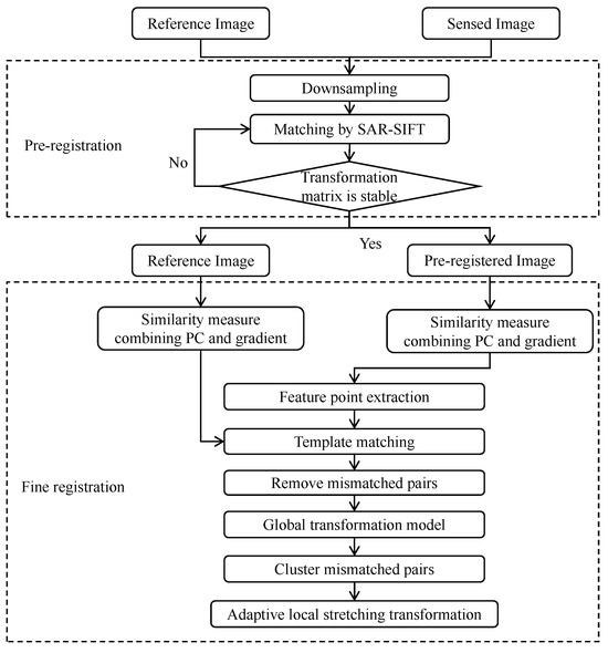
Figure 1.
The flowchart of the proposed method.
2.1. Pre-Registration
The SAR-SIFT algorithm represents one of the most widely adopted methods for SAR image registration, comprising three fundamental processing stages: feature point detection, principal orientation assignment and descriptor construction, and feature point matching. Distinct from conventional SIFT, SAR-SIFT does not construct a Difference of Gaussian (DoG) pyramid. Instead, it establishes a Harris scale space through the integration of Gaussian filtering with Harris corner detection. A critical modification involves substituting the standard gradient computation with the ROEWA operator, which is given as follows:
where I represents the input image, represents the coordinates, R represents the radius, and represent the positive and negative radius regions, respectively, represents the current scale, and are the edge strengths in the horizontal and vertical directions calculated using the ROEWA algorithm.
The constructed Harris matrix and corner response function are given as follows:
where represents a Gaussian kernel with a standard deviation of , tr(·) and det(·) represent the trace and determinant of , respectively, and the value of d is set to 0.04.
Feature points are subsequently identified as local extrema of across multiple scales. This approach reliably selects stable feature points in SAR imagery due to the ROEWA operator’s inherent noise robustness. By computing gradients within localized regions, ROEWA effectively suppresses multiplicative noise interference, a critical advantage for SAR image processing where speckle noise predominates.
To ensure rotation invariance, each feature point is assigned a principal orientation corresponding to the dominant peak in the gradient direction histogram within its characteristic scale space. The circular neighborhood and gradient direction histogram are used to construct the descriptor. For keypoint matching, an affine transformation model is adopted, with final correspondences determined through a combination of the nearest neighbor distance ratio (NNDR) and FSC method.
The pre-registration stage initiates with image downsampling, where an initial alignment is obtained through the SAR-SIFT algorithm. However, conventional global transformation estimation based on feature point matching often yields lower registration accuracy, and the downsampling process further exacerbates matching errors. Therefore, we propose an iterative refinement approach that progressively updates the pre-registered results. In this framework, the pre-registered image obtained from the SAR-SIFT algorithm replaces the current image to be matched and participates in the next round of matching. The process terminates when predefined convergence criteria are satisfied, indicating stabilization of the registration parameters. Following this iterative optimization on the downsampled image, the final matching pairs are mapped back to the original resolution to compute the transformation matrix. The geometric relationship between images is modeled using an affine transformation, expressed as
where are the affine transformation coefficients, and are the coordinates before and after the transformation, respectively. Chen et al. [27] defined a similarity value for reference image and sensed image. The iteration is cancelled when the difference between the maximum value of the similarity value of the k and times or the number of iterations is greater than the maximum allowed number of iterations, where is the set threshold. For the pre-registered image, a strict iteration termination condition is not necessary. Transformation stability can be assessed by analyzing coordinate convergence-diminishing displacements between original and transformed coordinates indicate stabilization. Conversely, significant displacements suggest unreliable matching pairs. This behavior manifests mathematically as the transformation matrix asymptotically approaching the identity matrix. Consequently, iterative control can be effectively implemented by constraining the affine transformation coefficients within predefined thresholds. Specifically, iterations cease when the coefficients satisfy && or when the iteration count is greater than the maximum number of iterations . The coefficients and f have the same constraints as and c, respectively.
2.2. Fine Registration
In the pre-registration stage, we eliminate significant scale, rotation, and translation differences between the reference image and the pre-registered image, and achieve rough alignment of the image. This allows the fine registration stage to focus on local feature matching. To ensure spatially uniform feature distribution, we implement a block-wise processing scheme where Harris corner detection is performed independently within each image partition. A similarity measure combining phase congruency and gradient is then employed for template matching, with mismatched pairs removed via FSC to obtain the global transformation model. Finally, mismatched pairs are clustered to identify terrain-undulated regions, where boundary sampling and local template matching determine stretching ratios for precise correction.
2.2.1. Feature Point Extraction
The fine registration stage initiates with feature point extraction from the pre-registered image. While conventional approaches typically employ DoG pyramid extrema (as in SIFT) or Harris corner detection (as in SAR-SIFT), this study adopts the latter approach due to its superior noise robustness in SAR image processing. However, Harris corners extract feature points by setting a threshold, which makes it difficult to control the number of feature points and often leads to an uneven distribution of feature points across the image. To address this issue, feature points are extracted by partitioning the pre-registered image into blocks. If a fixed pixel threshold method is adopted, the large-sized image will lead to more divided blocks, thus resulting in a larger number of feature points. Therefore, we employ a fixed number of blocks method, which can fix the quantity of blocks and feature points, avoid an excessive or insufficient number of feature points, and ensure the uniform global distribution of feature points. First, the image is partitioned into nonoverlapping blocks, and the Harris response values are calculated for each block. Subsequently, the Harris values within each block are sorted in descending order, and the top k points with the highest response values are selected as feature points. In the comparative methods, feature point selection is independent of a k-value, and a block-wise uniform distribution strategy is not employed. The number of feature points is determined by the algorithm itself. An example of feature points extracted using this method is shown in Figure 2b, the red dots denote feature points and it can be observed that the block-based approach ensures a uniform distribution of feature points across the image. The comparison with traditional threshold-based extraction (Figure 2a) clearly demonstrates the enhanced spatial distribution achieved by the block-wise approach.
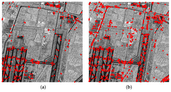
Figure 2.
Harris feature point extraction results. (a) Feature points extracted with fixed threshold. (b) Feature points extracted in blocks. (The red dots denote feature points.)
2.2.2. Similarity Measure Method Combining Phase Congruency and Gradient
Phase congruency detects image edges in the frequency domain, whereas ROEWA acquires image edges in the spatial domain. Taking these two approaches into account, this paper proposes a novel similarity measure method by integrating them.
First, the traditional phase congruency model is introduced. Unlike classical gradient-based operators for feature extraction, features can be perceived at points where the Fourier components have maximum phase. Venkatesh et al. demonstrated in [28] that the local energy model is proportional to phase congruency. Therefore, peaks in local energy correspond to peaks in phase congruency. The local energy is calculated by convolving the image with a bank of orthogonal filters. The calculation formula is provided in [11] as follows:
where n represents the number of scales, I denotes the image intensity, and represent the even-symmetric and odd-symmetric filters at scale n, denotes the convolution of the image with the even-symmetric filter, denotes the convolution of the image with the odd-symmetric filter, is the amplitude at scale n, and is the corresponding phase. To extend the local energy model to two dimensions, Kovesi improved the model by using log Gabor wavelets to compute local energy across scales and orientations. Then, considering image noise and blur, the phase congruency model proposed by Kovesi is defined as
where n represents the number of scales, o denotes the number of orientations, represents the weighting function at the o-th orientation, is the amplitude at scale n and orientation o, is the noise level at the o-th orientation, and is a small positive value to prevent the expression from becoming unstable when becomes very small. It is noted that at points of phase congruency, the cosine of the phase deviation should be large, while the absolute value of the sine of the phase deviation should be small. The gradient of the sine function is maximum at the origin. Therefore, use the sine of phase deviation to increase sensitivity.
For Equation (10), for a specific orientation, its meaning is the phase congruency in that orientation, obtaining the edge in that direction. As for Equation (12), its meaning is the edge in a specific orientation after o takes a determined value. For example, if a total of 6 orientations are taken, the value of o is , with an orientation interval of 180°/6 = 30°, and the orientations are 30°.
The method for calculating edge gradients in the spatial domain is similar to this idea. For edges in different orientations, there is a corresponding computational method in the spatial domain, which is defined as
where I represents the input image, represents the coordinates, o represents the orientation, and represent the positive and negative radius regions in the o orientation, respectively, represents the current scale, and represent the positive and negative regional means in the o orientation, respectively. represents the edge strength in the o direction.
By combining the gradient calculation results from the frequency domain and the spatial domain for a specific direction, new edge information can be obtained, denoted as , which is defined as
Similar to the normalized cross-correlation (NCC) method, the NCC of (denoted as ) is used as the similarity measure for image registration. It is defined as
where E and T represent the responses of the pre-registered image and the template image, respectively, is the mean value of T, denotes the mean value of E over the region corresponding to the template size, and are the coordinates of the feature points in the pre-registered image. For each feature point in the pre-registered image, the similarity of all pixel points within the local region corresponding to the template image is calculated, and the point with the highest similarity forms a candidate matching pair.
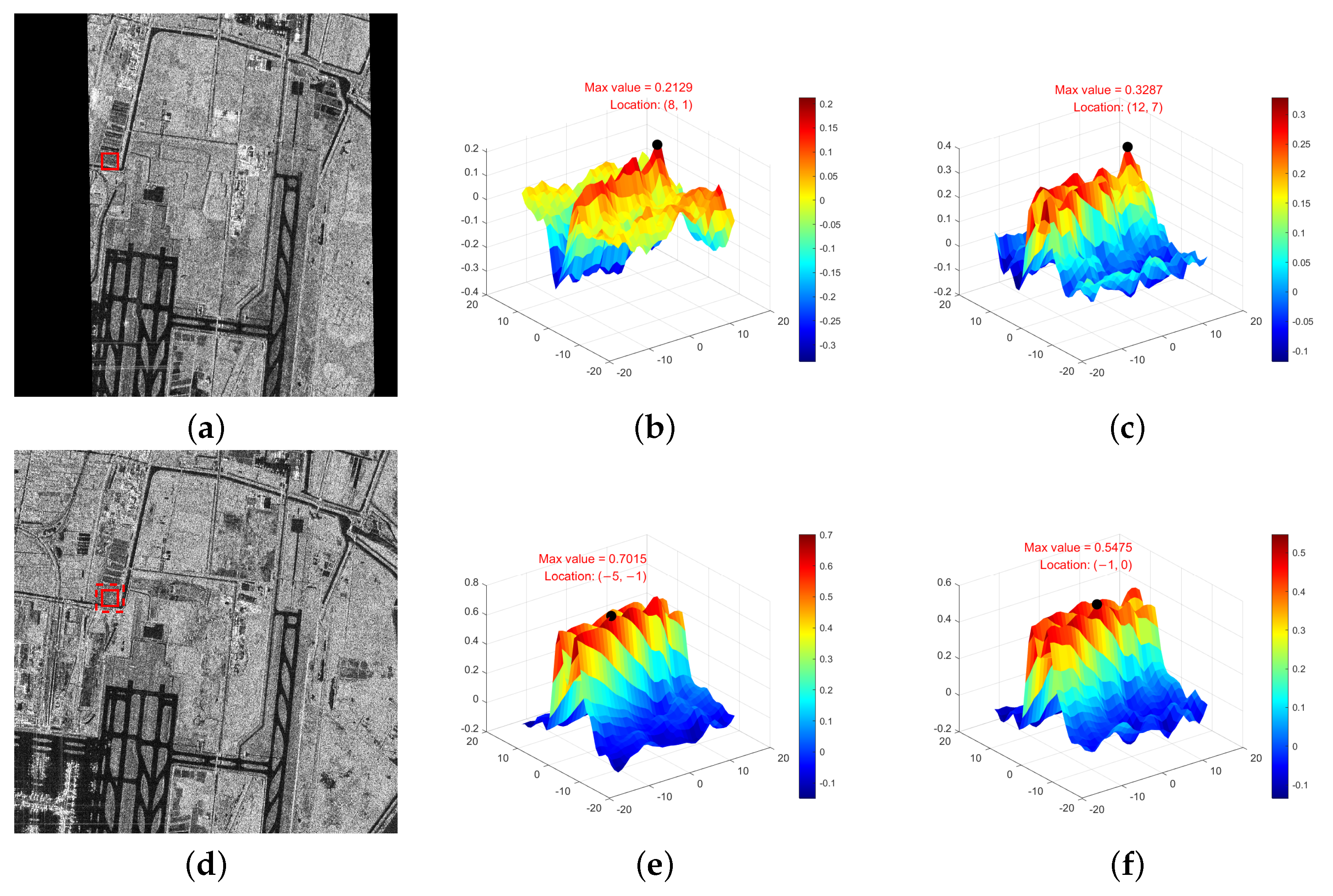
To validate the matching performance of the proposed similarity measure, we compared it with the NCC of image intensity, the NCC of PC, and the NCC of edge strength (Gra, obtained using ROEWA) through similarity curves. Template matching experiments were conducted on the fine registered image and the reference image. A region of size was selected in the fine registered image, and a search was performed within the local range of the corresponding point in the reference image, with the search range set to . The two-dimensional similarity curves for the four comparison methods are shown in Figure 3, with peaks marked in each curve. Among them, (a) is the fine registered image, (d) is the reference image, the red solid frame indicates the corresponding region used for testing, and the red dashed frame in (d) represents the search range. The correct position is located at the center of the search region. (b) shows the NCC using image intensity, with the optimal position at (8, 1) and the maximum similarity value of 0.2129; (c) shows the NCC using PC, with the optimal position at (12, 7) and the maximum similarity value of 0.3287; (e) shows the NCC using Gra, with the optimal position at (, ) and the maximum similarity value of 0.7015; (f) shows the proposed PCGCC, with the optimal position at (, 0) and a maximum similarity value of 0.5475. It can be observed that the proposed method achieves relatively accurate results. Further analysis of these four methods and the impact of template size is provided in Section 3.

Figure 3.
Comparison of similarity curves: (a) The fine registered image. (b) NCC of image intensity. (c) NCC of PC. (d) The reference image. (e) NCC of Gra. (f) PCGCC.
2.2.3. Local Correction for Terrain-Undulated Areas
After global correction transformation, the registered image and the reference image achieve precise registration in flat regions. However, due to the effects of side-looking imaging, correct matching pairs in terrain-undulated areas may not satisfy the final global transformation model. Therefore, the first step is to identify matching pairs that do not conform to the final transformation model and cluster these pairs using the density-based DBSCAN algorithm to obtain different clusters, which are regarded as candidate terrain-undulated regions. Subsequently, an adaptive local stretching transformation is performed in accordance with the following steps:
- Determination of rectangular bounding boxes for candidate terrain-undulated regions: For the candidate terrain-undulated regions obtained through DBSCAN clustering, feature points are resampled, and template matching is re-performed to obtain new matching pairs. Based on the distribution characteristics of these matching pairs, the transformation ranges in the x and y directions are calculated, and rectangular bounding boxes are constructed for each candidate region. If the newly obtained matching pairs satisfy the final transformation matrix, it indicates that the candidate region is not a terrain-undulated region and will be excluded from subsequent correction processes.
- Sampling and detection of terrain-undulated region boundaries: In both the x and y directions, dense sampling is performed starting from the center point of the rectangular bounding box, extending outward on both sides to detect the boundary positions of the terrain-undulated regions. For each sampling point, if it is located in a flat region, sampling proceeds toward the undulating region and vice versa. By analyzing the spatial distribution characteristics of the sampling points, the boundary regions of topographic relief are preliminarily identified, leading to a more precise boundary of the undulating area.
- Refined division of terrain-undulated regions: Based on the distance between boundary sampling points, a threshold is employed to determine whether adjacent sampling points belong to the same terrain-undulated region. If the distance exceeds the preset threshold, they are classified into independent regions; otherwise, they are regarded as part of the same continuous region. Through this procedure, the candidate terrain-undulated regions are further subdivided into multiple specific sub-regions.
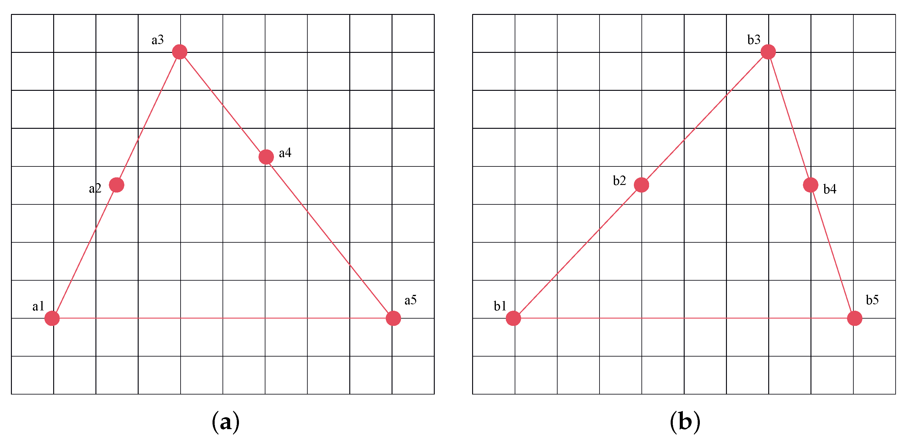
- Calculation of local stretching transformation ratios: For each subdivided terrain-undulated region, the local stretching transformation ratio is calculated based on the local transformation characteristics of matching pairs. Since most terrain-undulated regions are situated in mountainous areas with no distinct features, mismatches are prone to occur. In this step, uniform sampling is used to obtain matching pairs, and an affine transformation model is employed to preliminarily eliminate mismatches. The stretching transformation ratio is determined by the correct matching pair with the maximum transformation distance within the region, ensuring that the stretching transformation fully adapts to the local variation characteristics of the terrain-undulated region, thereby improving correction accuracy. As shown in Figure 4, a simplified top view of local transformation induced by topographic relief is shown, where points a1 and b1, a as well as points a5 and b5, denote the corresponding boundary regions, while a2, a3, a4 correspond to b2, b3, b4 as correct matching pairs. In this case, the transformation distances for these three correct matching pairs are 1.5, 3, and 2, respectively. The stretching transformation ratio is determined by matching pairs a3 and b3 with the largest transformation distances.
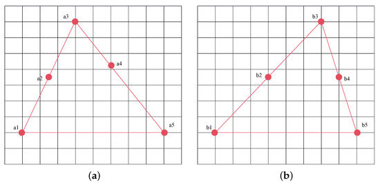 Figure 4. Example of stretching transformation in terrain-undulated regions: (a) Image to be corrected. (b) Reference image.
 - Application of adaptive local stretching transformation: Based on the calculated stretching transformation ratios, an adaptive local stretching transformation is applied to each terrain-undulated region. Taking the transformation in the x-direction as an example, the transformation formulas are given as follows:where and represent the left and right boundaries of the terrain-undulated region in the x-direction, respectively; and denote the x coordinates of the transformation pairs determined in step (4) for the pre-registered image and the reference image, respectively; and represent the stretching transformation ratios for the x direction. denotes the transformed coordinate at position x. The transformation in the y-direction follows the same principle as in the x-direction.
3. Results
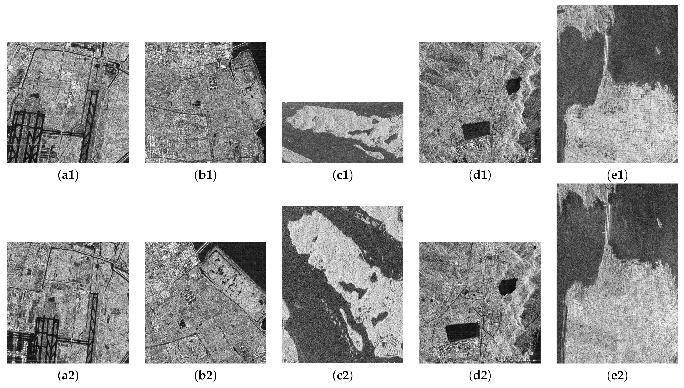
In this section, five pairs of polarimetric SAR images are used to evaluate the registration performance of the proposed method. The information about the test images is shown in Table 1. Image Pair 1 is Pudong, China, with both sensors being GF3, captured on 24 September 2021 and 11 November 2023, respectively. Both images have a resolution of 8 m × 8 m, with incidence angles of 23.9° and 35.5°, both in ascending pass direction, and dimensions of 1000 × 1000. Image Pair 2 is Taicang, China, also captured by GF3 sensors, on 24 September 2020 and 20 December 2021, respectively. Both images have a resolution of 8 m × 8 m, with incidence angles of 25.5° and 20.1°, in descending and ascending pass directions, respectively, and dimensions of 900 × 900. Image Pair 3 is Singapore, captured by TerraSAR-X and RADARSAT2 sensors on 10 March 2014 and 19 January 2013, respectively. The resolutions are 2.06 m × 6.59 m and 4.73 m × 4.80 m, with incidence angles of 34.7° and 46.7°, in descending and ascending pass directions, respectively, and dimensions of 685 × 1351 and 821 × 631. Image Pair 4 is Zhoushan, China, captured by GF3 sensors on 30 September 2018 and 20 November 2016, respectively. Both images have a resolution of 8 m × 8 m, with incidence angles of 30.8°and 25.2°, both in ascending pass direction, and dimensions of 900 × 900. Image Pair 5 is San Francisco, the United States, captured by ALOS2 and RADARSAT2 sensors on 24 March 2015 and 9 April 2008, respectively. The resolutions are 6 m × 6 m and 4.73 m × 4.82 m, with incidence angles of 30.8° and 28.0°, both in ascending pass direction, and dimensions of 2876 × 2205 and 1749 × 1180. In optics, color image matching will be converted into gray image for matching. Similarly, this paper converts polarization information into gray information and uses single-channel image for matching. The images used in the experiments are shown in Figure 5. Image Pairs 1 to 3 are flat areas, and Image Pairs 4 and 5 have terrain-undulated areas.

Table 1.
Image information: DEC is for the direction of descent, and ASC is for the direction of ascent.
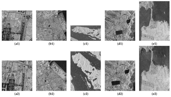
Figure 5.
Matching image pairs: (a1–e1) The sensed images of the five image pairs. (a2–e2) The corresponding reference images.
To objectively quantify the noise level of experimental images, we employed the Equivalent Number of Looks (ENL), a common speckle noise intensity evaluation index in SAR images, for assessment. A larger ENL indicates smoother images with weaker noise, whereas a smaller ENL signifies stronger speckle noise in the images. The ENL is calculated as: , where and are the pixel mean and variance of the selected homogeneous regions in the image, respectively. The ENL of Image Pair 1 are 4.37 and 4.62, respectively. The ENL of Image Pair 2 are 3.57 and 5.41, respectively. The ENL of Image Pair 3 are 5.67 and 6.07, respectively. The ENL of Image Pair 4 are 3.60 and 4.14, respectively. The ENL of Image Pair 5 are 5.69 and 5.38, respectively.
3.1. Parameter Settings
In the pre-registration stage, the threshold for the NNDR matching method is set to 0.9, while in the iterative matching process, , , , and are set to 0.05, 0.05, 1.5, and 20, respectively. The selection criteria for , , , and are analyzed in Section 3.3. In the fine registration stage, as detailed in reference [25], the positioning deviation of the pre-registered images is approximately set to 5 pixels, with the search area defined as , where s is the downsampling factor. Given that some matching pairs in pre-registration are relatively concentrated and unevenly distributed across the image, which may lead to larger positioning errors in regions farther from these pairs, and considering that this paper employs 2× downsampling, the local search area is adjusted to [−15, 15]. The pre-registered images obtained in the pre-registration stage are partitioned into 5 × 5 nonoverlapping image blocks, with k set to 25, which refers to the number of feature points per block. A larger k value will improve the accuracy of fine registration but will also significantly increase the computational cost. When constructing the similarity measure, a template size of is used, and the selection of r is analyzed in Section 3.4. In terms of DBSCAN parameter settings, the euclidean distance metric is adopted with a neighborhood radius set to 100 pixels, which ensures that sufficient discrete matching pairs can be captured in locally stretched areas induced by side-looking imaging, and minimum number of points is set to 10 matching pairs, which avoids false detection due to too few points (e.g., noise point clustering) while ensuring effective identification of small-scale terrain-undulated regions. The similarity measure threshold is an adaptive threshold defined as the median of the optimal similarity values of all feature points. This approach reduces the number of low-similarity matching pairs by half, thereby minimizing the impact of mismatches on registration accuracy.
3.2. Evaluation Criteria
The number of matching pairs(NMP), root mean square error (RMSE, in pixels), and running time (in seconds) are used to evaluate the performance of the proposed method, where the RMSE is defined as follows:
where represents the corresponding coordinates of after applying the transformation matrix. and represent the correct matching pairs that are manually identified, and N represents the total number of correct matches manually identified. For each image pair, 16 sets of correctly matched pairs are manually determined.
3.3. Effectiveness of Iterative Matching in Pre-Registration Stage
, , , and control the number of iterations (NOI). In the experiments, we found that the linear parameters a, b, d, and e converged rapidly within 0.05, whereas c and f exhibited larger fluctuations, making the range of the primary control factor. Table 2 presents the NOI and RMSE results for five image pairs under different settings (1, 1.5, 2, and 2.5). As shown in Table 2, higher values relax the constraints, leading to a downward trend in NOI. Specifically: When = 1, Image Pairs 2, 3, and 4 required significantly more iterations. When = 1.5, only Image Pair 2 had a high NOI, while the NOI for other images was effectively reduced, with good RMSE performance maintained. When = 2, the NOI for Image Pair 2 decreased by only 2, with no changes for the rest. When = 2.5, the RMSE for Image Pair 2 reached 20.19, indicating a large deviation. Considering both convergence speed and RMSE, was ultimately set to 1.5. The maximum iteration count was primarily determined by referencing the strictest setting ( = 1), where the maximum iteration count was 15. Therefore, we set = 20.
Table 2.
Influence of on NOI and RMSE.
Table 3 shows the NOI, original RMSE, and final RMSE for the five image pairs in the pre-registration stage. From the results, it can be observed that for Image Pairs 1 and 5, the final RMSE decreased slightly compared with the original values, dropping from 2.26 and 7.68 to 2.18 and 7.13, respectively. For Image Pairs 3 and 4, the final RMSE increased slightly compared with the original values, rising from 5.19 and 4.35 to 6.87 and 5.07, respectively. For these four image pairs, the change in final RMSE compared with the original values was insignificant, with the NOI remaining relatively low (5 or fewer). However, Image Pair 2 exhibited a notable decrease in final RMSE, dropping from 25.73 to 6.10, and the NOI was 11. The results show that the performance of iterative matching in the pre-registration stage is not obvious for images with good original matching results, while for images with poor original matching results, iterative matching can effectively transform and correct the images, avoiding high registration errors and, at the same time, the NOI will be greater.
Table 3.
Influence of iterative matching on RMSE in pre-registration stage. (Boldface indicates the best results, and this convention is maintained in the subsequent sections.)
3.4. Effectiveness of the Proposed Similarity Measure Method
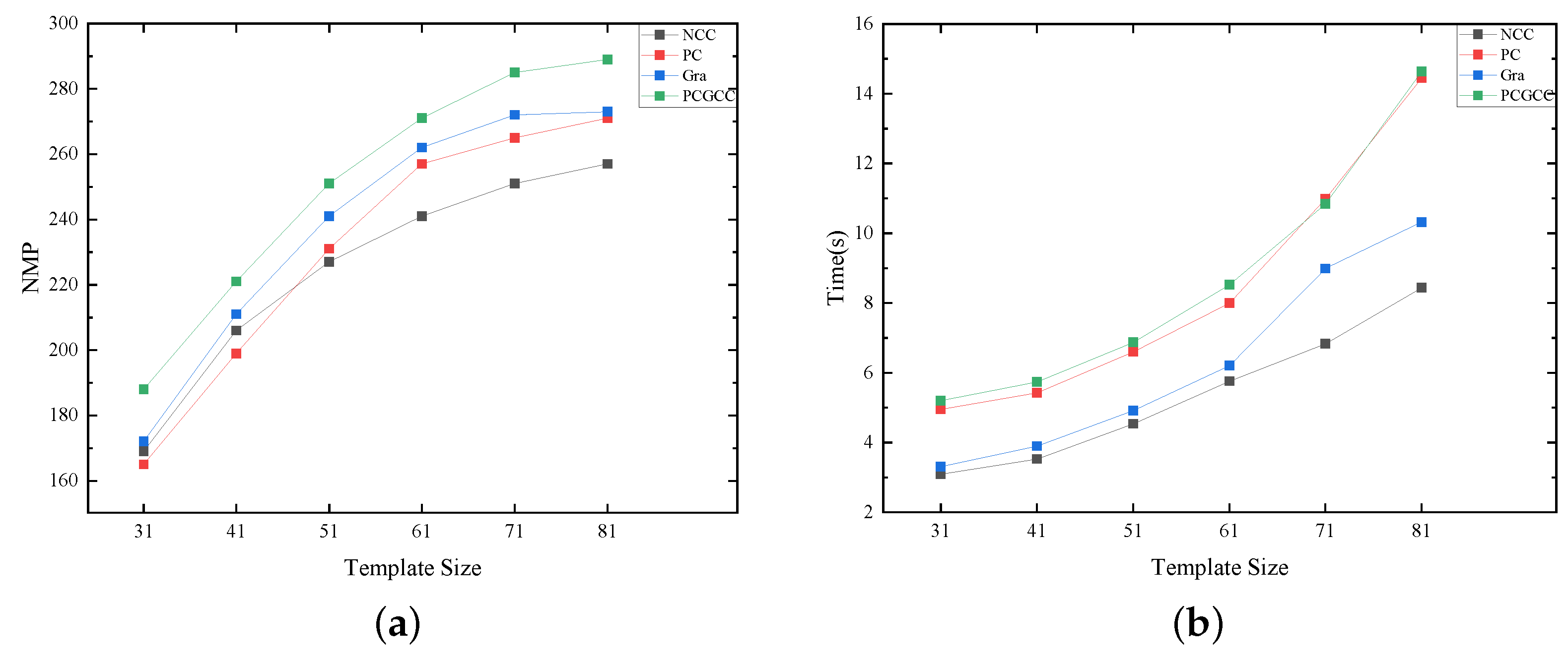
In template matching, we propose a new similarity measure method, PCGCC. The template size significantly impacts the matching results. Smaller template regions typically lack sufficient structural information, making them prone to matching ambiguities or mismatches. Larger templates can contain more image structural features, enhancing the robustness and accuracy of the similarity measure. Consequently, the template size is set within the range of 31 × 31 to 81 × 81. This paper analyzes the impact of template size on the performance of four similarity measure methods using Image Pair 1, as shown in Figure 6. Firstly, for all four similarity measure methods, as the template size increases, both the NMP and the running time increase. Larger templates mean more structural information, which improves the uniqueness of the similarity measure, and requires longer running time. Compared with other similarity measure results, the proposed method obtains more matching pairs across different template sizes but has the longest running time. In terms of the NMP, there is a noticeable increasing trend within the range of 31 × 31 to 71 × 71, reaching a near-maximum value at 71 × 71, after which the growth rate diminishes and stabilizes. In terms of running time, the growth is stable from 31 × 31 to 71 × 71 but rises sharply at 81 × 81. Given that subsequent steps require mismatched pairs to correct terrain-undulated regions, we intend to use as large a template as possible to reduce the number of mismatched pairs. Balancing the running time, we set the template size to 71 × 71.
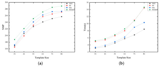
Figure 6.
Comparison of NCC, PC, Gra, and PCGCC on Image Pair 1: (a) NMP and template size. (b) Running time and template size.
Table 4 shows the NMP for four similarity measure methods across five image pairs. The experimental results show that the proposed PCGCC method outperforms the individual PC and Gra methods in all five image pairs, achieving 285, 103, 164, 235, and 228 correct matching pairs, respectively, showing its significant advantage in feature matching. Compared with the NCC method, which directly utilizes image intensity, PCGCC performs better in the first four image pairs (285, 103, 164, and 235, respectively) than NCC (251, 82, 101, and 204, respectively). However, in Image Pair 5, the NCC method obtains 265 correct matches, outperforming PCGCC’s 228 matches. Through analysis, it is found that Image Pair 5 is dominated by vegetation areas with minimal human influence. Except for coastal edges, the inner edge of the land is not obvious, which makes the direct use of image intensity information more stable than relying on edge information. In contrast, Image Pairs 1, 2, and 4 are significantly influenced by human activities, exhibiting obvious edge information. For Image Pair 3, although it contains few artificial structures, the land areas have highly distinct edge structures. Therefore, in these images, the edge information extracted by PCGCC proves more stable than image intensity information. These experimental results show that the proposed PCGCC method extracts more stable edge information and achieves better matching performance compared with phase congruency in the frequency domain and image gradients in the spatial domain. However, in images with fewer artificial regions and less distinct edge information, intensity-based methods can get better results.
Table 4.
The NMP for four similarity measure methods across five image pairs.
3.5. Effectiveness of Adaptive Local Stretching Transformation
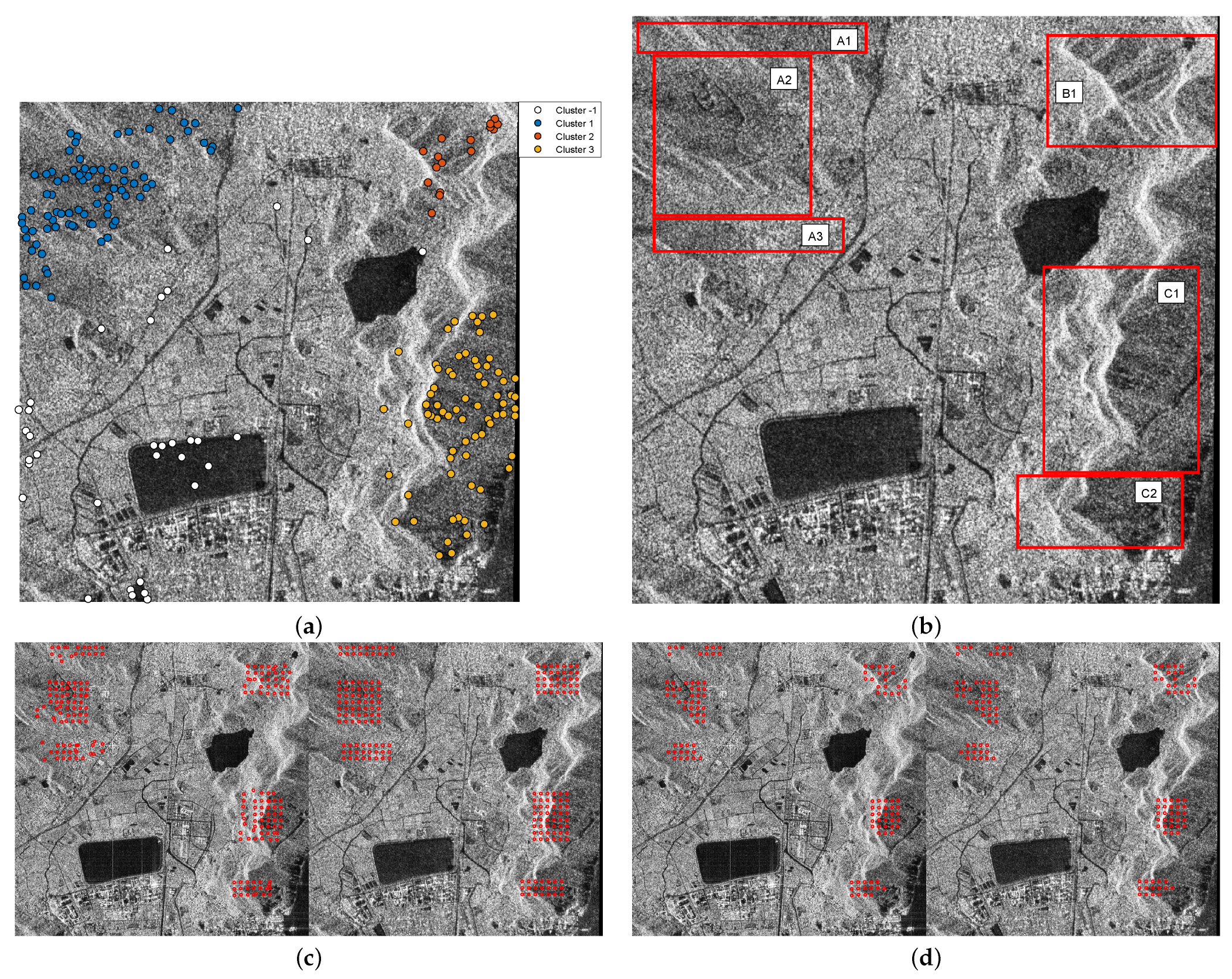
The effectiveness of the adaptive local stretching transformation is discussed using Image Pair 4 as an example. In this approach, the terrain-undulated regions are identified after the fine-registered global transformation, and the adaptive local stretching transformation is carried out. Figure 7 shows the steps and the results of the adaptive local stretching transformation. In (a), the points represent matching points that do not satisfy the final transformation matrix, and DBSCAN is employed to obtain four groups of results: −1 represents feature points that do not belong to any cluster, while 1 to 3 represent three groups of feature points, each determining a candidate terrain-undulated area. In (b), the boundaries of each candidate terrain-undulated area are sampled and divided to obtain more precise terrain-undulated regions. For instance, the first area is divided into three regions (A1, A2, and A3); the second candidate area remains as a single region (B1); and the third area is divided into two regions (C1 and C2). In (c), the results of sampling feature points and calculating matching points for each refined region are shown, where notable mismatched pairs are observable. In (d), the results of using affine transformation to roughly remove mismatched pairs are shown. This step can effectively avoid the influence of mismatched pairs on the subsequent stretching transformation.

Figure 7.
Results of adaptive local correction process: (a) Grouping of feature points. (b) Refinement of local undulating region. (c) Sampling and matching of feature points. (d) Affine transformation of matching pairs.
After finding the feature points and matching pairs, the matching pair with the maximum transformation distance is selected to calculate the stretching transformation ratio. Table 5 shows the correction results of the adaptive local stretching transformation for Image Pairs 4 and 5. For Image Pair 4, three candidate terrain-undulated regions are initially identified, and the final number of refined terrain-undulated regions is six. As shown in Figure 7b, the maximum transformation distances for regions A1, A2, and A3 are 9, 11, and 2, respectively. It can be observed that although regions A2 and A3 are adjacent, the maximum transformation distance of A3 is significantly lower than that of A2, which partly shows that the topographic relief of region A3 is low, which is consistent with the fact. The maximum transformation distance for the B1 region is 16. The maximum transformation distances for regions C1 and C2 are 25 and 18, respectively. For Image Pair 5, two candidate terrain-undulated regions were initially identified, but finally, only one terrain-undulated region remains. This is because after sampling and matching with feature points, one region satisfies the final transformation matrix, indicating that the region does not need to be corrected. The maximum transformation distance for the remaining region is 6. The local correction times for the two image pairs are 52.92 s and 13.59 s, respectively. Image Pair 4 exhibited a longer running time than Image Pair 5 due to its higher number of terrain-undulated regions, which inherently require more processing time.
Table 5.
Correction results of adaptive local stretching transformation for Image Pairs 4 and 5. (CRR is for candidate undulating region. FRR is for final undulating region. MTD is for maximum transformation distances.)
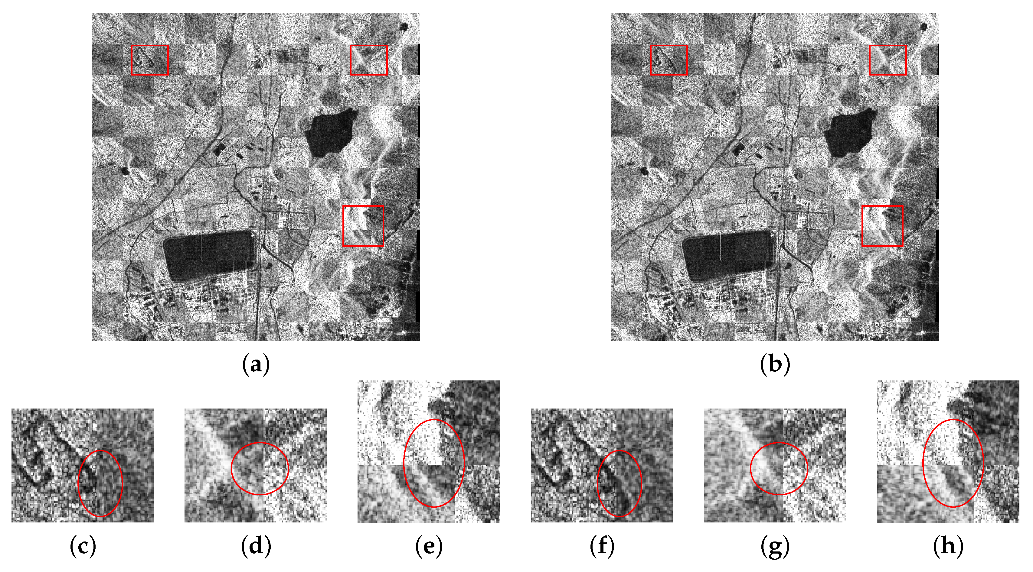
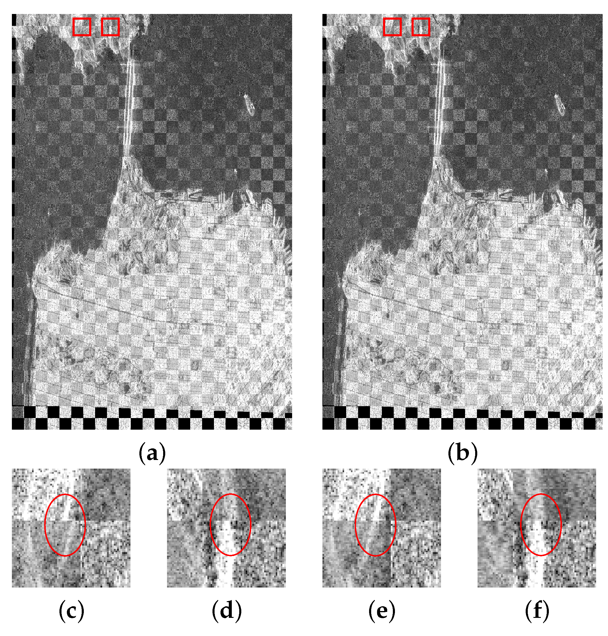
Figure 8 and Figure 9 utilize checkerboard images to show the correction results for terrain-undulated regions in Image Pairs 4 and 5. In Figure 8, (a) shows the global transformation results of fine registration; (b) shows the local stretching transformation results of fine registration; (c–e) display the first, second, and third sub-images of the global transformation results for the terrain-undulated regions; and (f–h) show the corresponding first, second, and third sub-images of the local stretching transformation results for the terrain-undulated regions. In Figure 9, (a) shows the global transformation results of fine registration; (b) shows the local stretching transformation results of fine registration; (c,d) show the first and second sub-images of the global transformation results for the terrain-undulated regions; and (e,f) show the corresponding first and second sub-images of the local stretching transformation results for the terrain-undulated regions. From the checkerboard images, it can be observed that after the global transformation of fine registration, the deviations remain significant in the terrain-undulated regions, with obvious edge discontinuities. However, after applying the adaptive local stretching transformation, the edge connections in the terrain-undulated regions become smoother, leading to a notable improvement in registration accuracy.
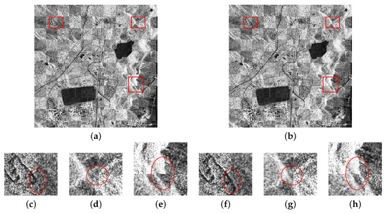
Figure 8.
Correction results of the undulating region of Image Pair 4: (a) Fine registration global transformation results. (b) Fine registration local stretching transformation results. (c–e) The first, second, and third sub-images of global transformation. (f–h) The first, second, and third sub-images of local stretching transformation. (Where the rectangular box represents the sub-image area and the circular box represents the edge-connected area of the corrected image and the reference image, and this convention is maintained in the subsequent sections.)
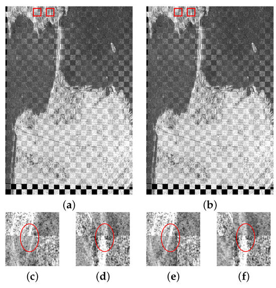
Figure 9.
Correction result of the undulating region of Image Pair 5: (a) Fine registration global transformation results. (b) Fine registration local stretching transformation results. (c,d) The first and second sub-images of global transformation. (e,f) The first and second sub-images of local stretching transformation.
3.6. The Registration Performance of the Proposed Method
For the matching method proposed in this paper, this section performs an intuitive inspection through checkerboard mosaic images and enlarged sub-images, and analyzes it with quantitative indicators.
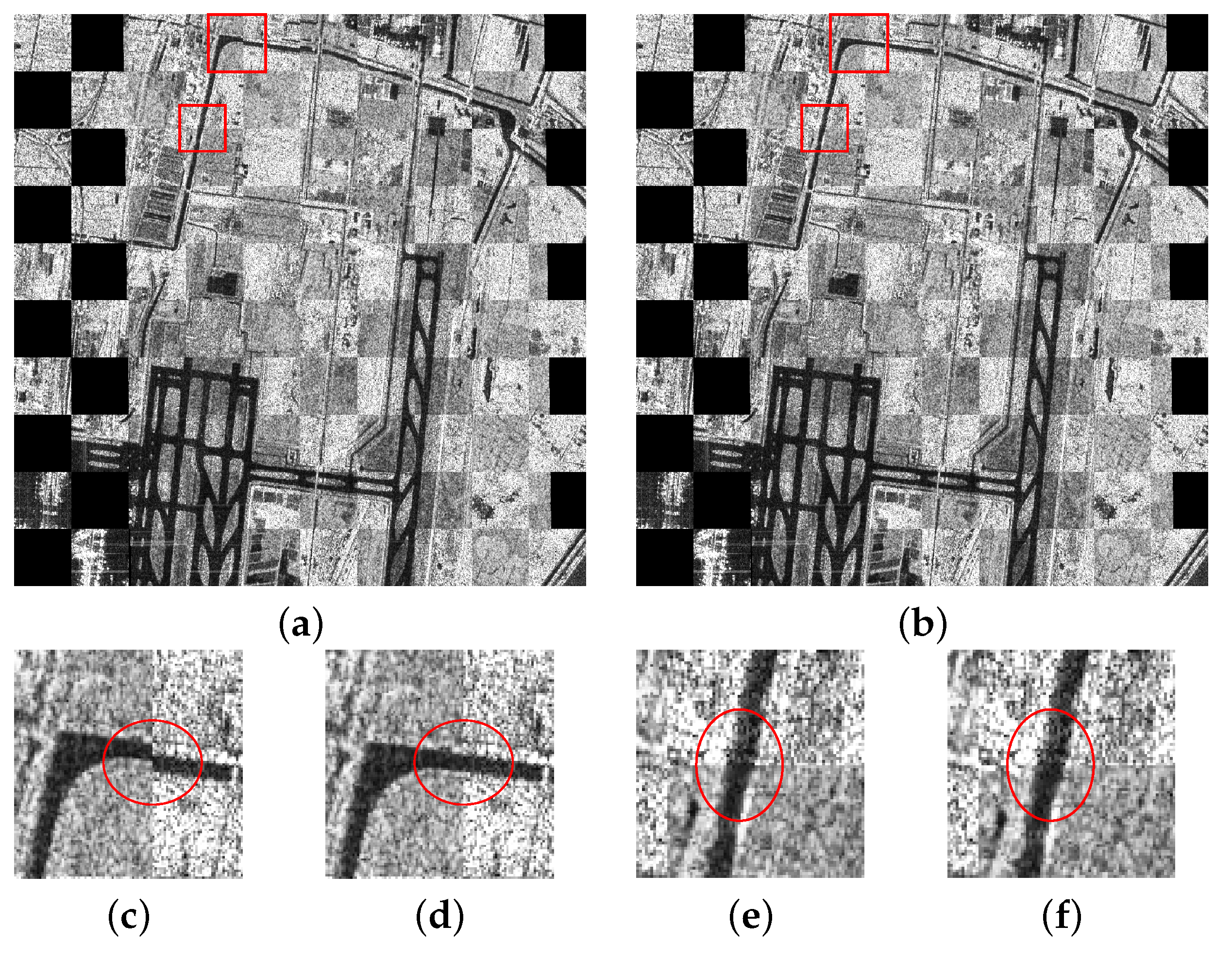
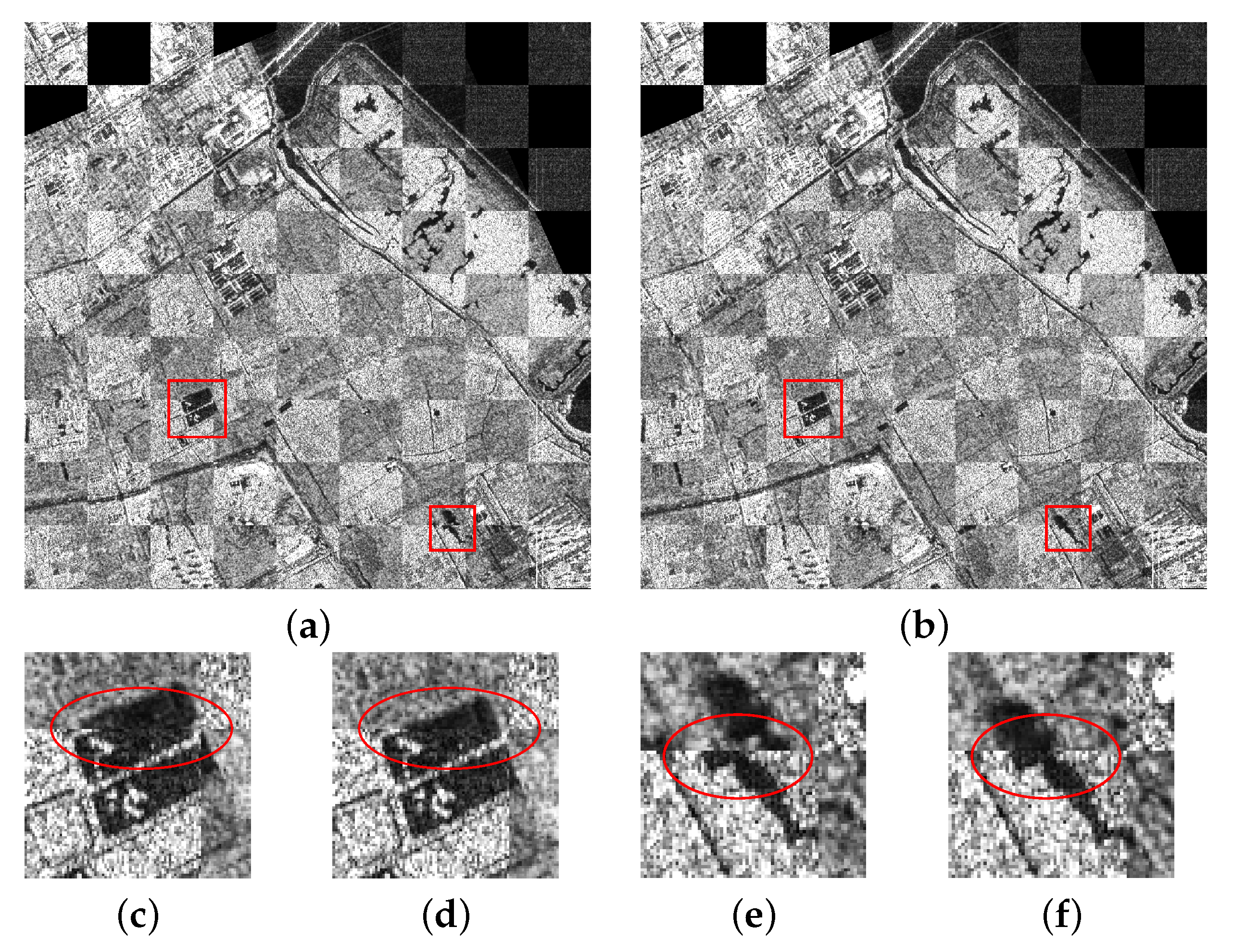
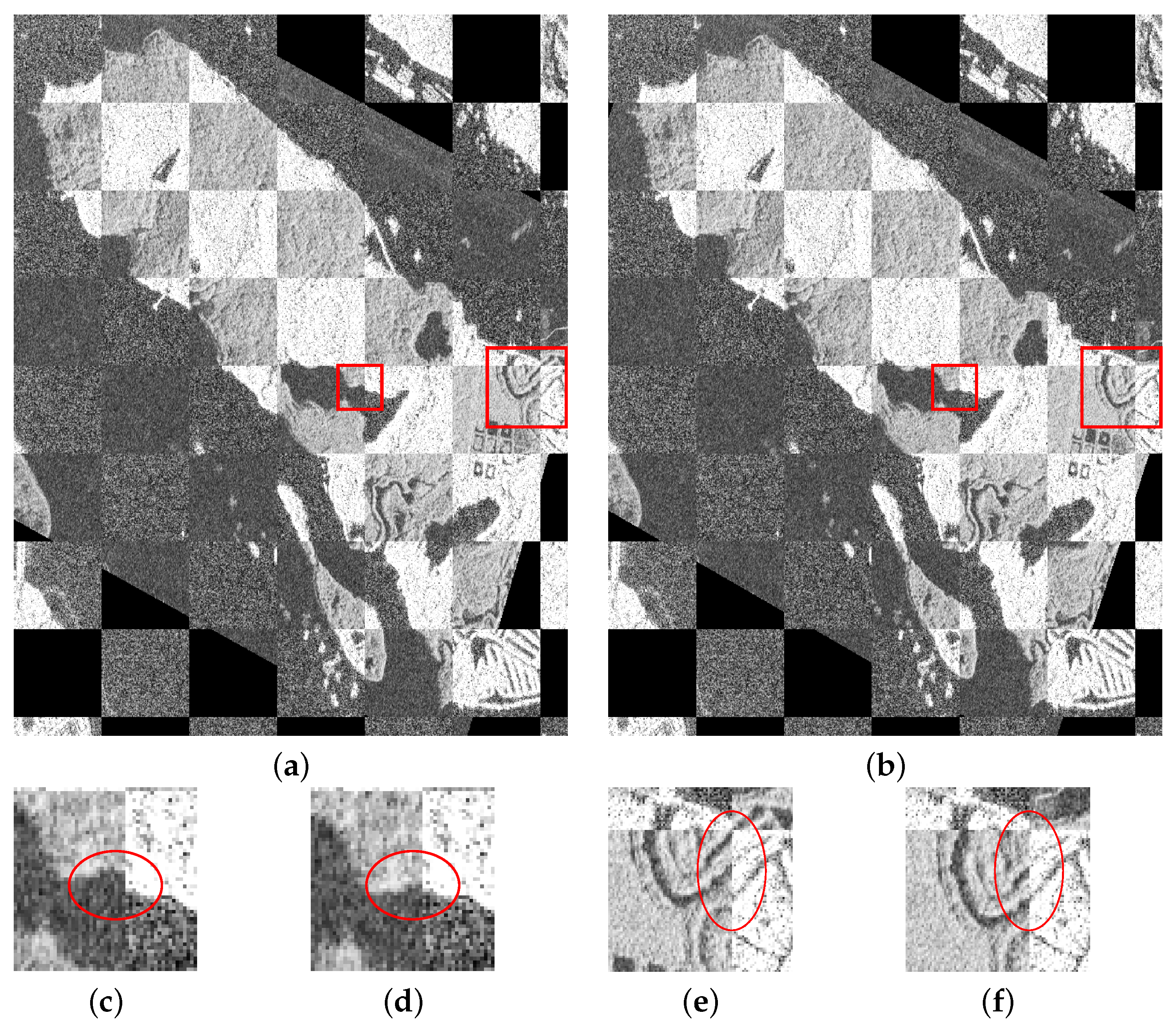
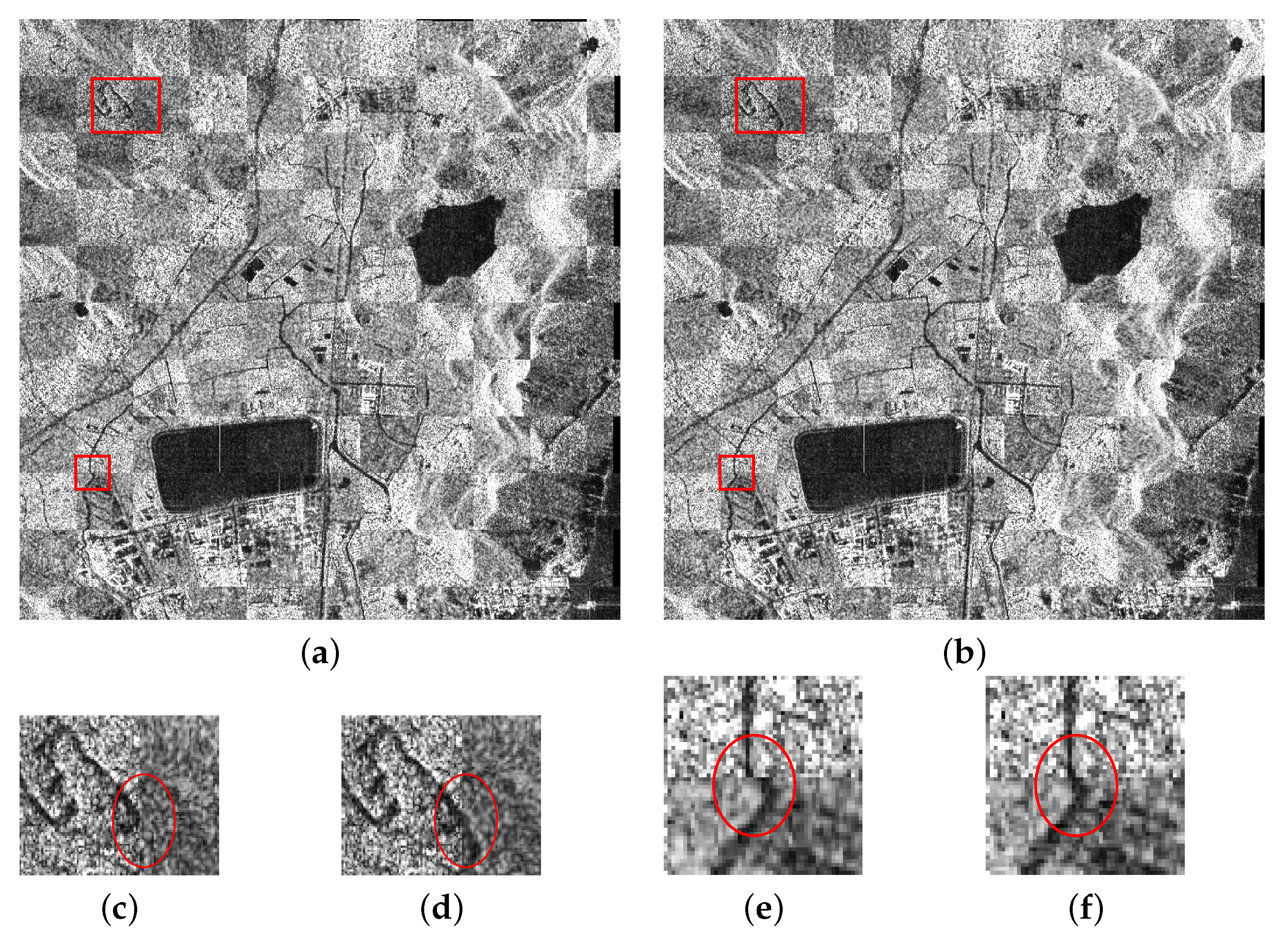
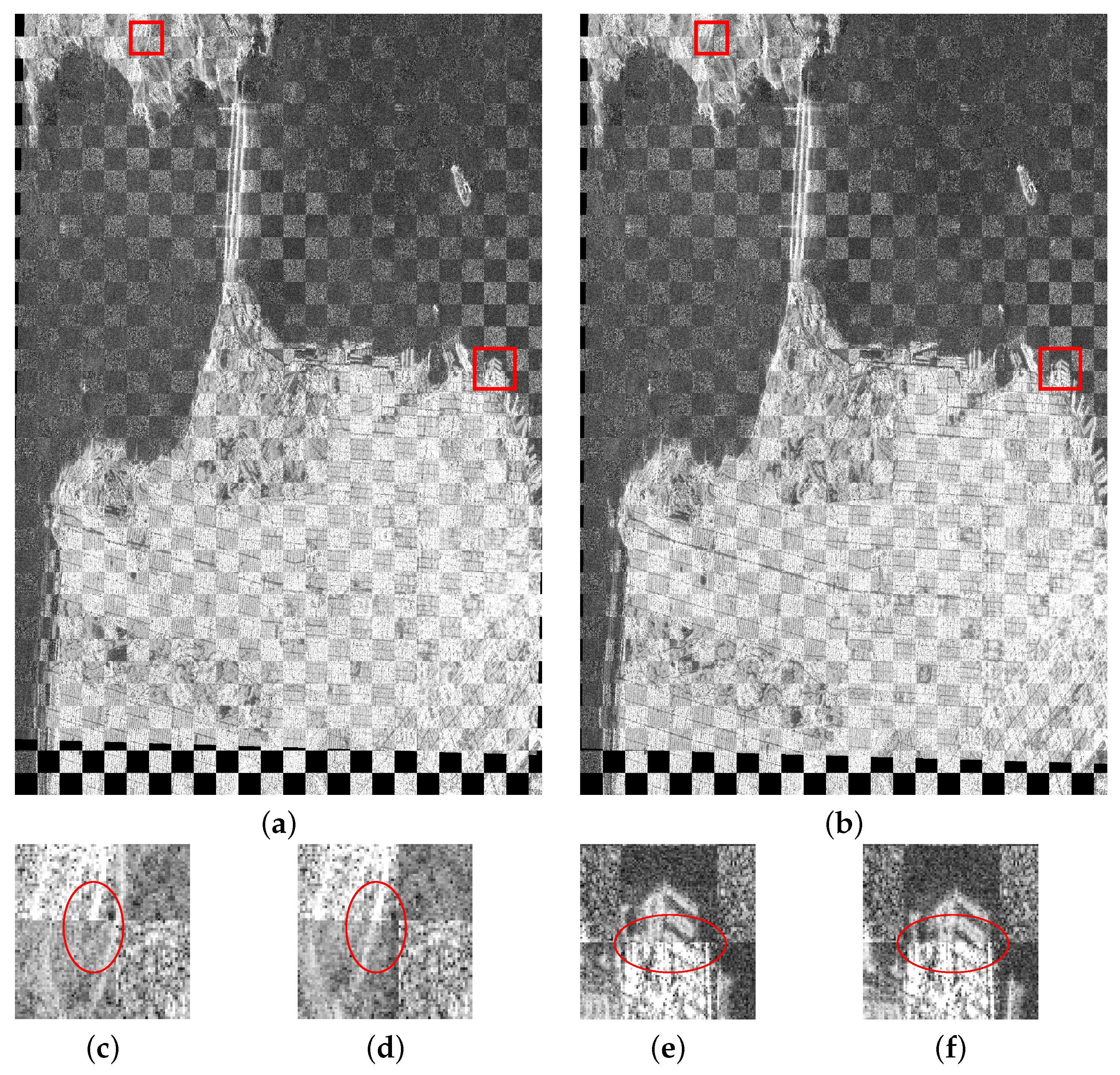
The first comparison is between fine registration and pre-registration, where fine registration refers to the registration result corrected by global correction and adaptive local stretching transformation. In the experiment, to facilitate a clearer comparison between the adjacent checkerboards of the pre-registered image and the reference image, the intensity of the reference image is proportionally amplified. Figure 10, Figure 11, Figure 12, Figure 13 and Figure 14 show the pre-registration and fine registration results for the five image pairs, along with enlarged sub-images. It can be intuitively observed from the results that in the pre-registration stage, although the pre-registered images and reference images are roughly aligned, there are still deviations in details, which are particularly obvious at the edges, as shown in (c) and (e) of Figure 10, Figure 11, Figure 12, Figure 13 and Figure 14. In the fine registration stage, PCGCC is employed as the similarity measure to identify correct corresponding points within the local search area, followed by corresponding corrections to the pre-registered images. The enlarged sub-images of the same region in the fine registration results are shown in (d) and (f) in Figure 10, Figure 11, Figure 12, Figure 13 and Figure 14. Compared with the pre-registration results, the edge connections exhibit notably higher accuracy. As can be observed from Table 6, the fine registration stage obtained a significantly higher NMP and fewer pixel errors compared with the pre-registration stage. In terms of NMP, the pre-registration stage obtained 25, 10, 7, 11, and 6 matching pairs for the five image pairs, respectively, whereas the fine registration stage obtained 285, 103, 164, 235, and 228 matching pairs, respectively. Additionally, in terms of RMSE, the pre-registration stage exhibited values of 2.18, 6.10, 6.87, 5.07, and 7.13, respectively, while the fine registration stage achieved RMSE values of 0.55, 0.74, 0.69, 0.66, and 0.85, respectively, all below 1. This clearly indicates that the fine registration stage produces more accurate registration results. In terms of running time, the two stages employ different algorithms, so their time costs do not exhibit a strictly linear relationship. The runtime for Image Pairs 1–3 in the pre-registration stage is longer than that in the fine registration stage. This is because multiple rounds of feature matching and transformation updates may be required to obtain stable registration results in the pre-registration stage, leading to relatively longer time consumption for this stage. The fine registration stage, directly based on the pre-registration results, performs a one-time local search, so the calculation process is relatively fixed and efficient. The reason why the fine registration stage of Image Pairs 4–5 takes longer is the need for correction in terrain-undulated areas.
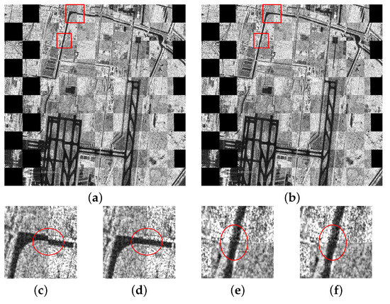
Figure 10.
Registration results of Image Pair 1: (a) Pre-registration results. (b) Fine registration results. (c) The first sub-image of pre-registration. (d) The first sub-image of fine registration. (e) The second sub-image of pre-registration. (f) The second sub-image of fine registration.
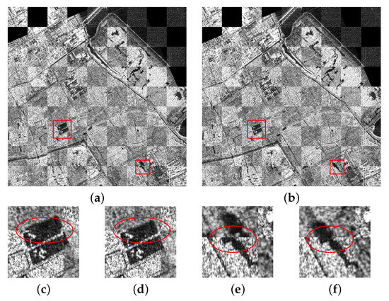
Figure 11.
Registration results of Image Pair 2: (a) Pre-registration results. (b) Fine registration results. (c) The first sub-image of pre-registration. (d) The first sub-image of fine registration. (e) The second sub-image of pre-registration. (f) The second sub-image of fine registration.

Figure 12.
Registration results of Image Pair 3: (a) Pre-registration results. (b) Fine registration results. (c) The first sub-image of pre-registration. (d) The first sub-image of fine registration. (e) The second sub-image of pre-registration. (f) The second sub-image of fine registration.
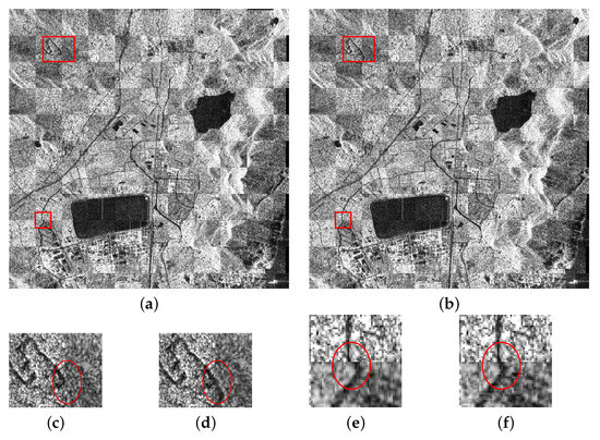
Figure 13.
Registration results of Image Pair 4: (a) Pre-registration results. (b) Fine registration results. (c) The first sub-image of pre-registration. (d) The first sub-image of fine registration. (e) The second sub-image of pre-registration. (f) The second sub-image of fine registration.
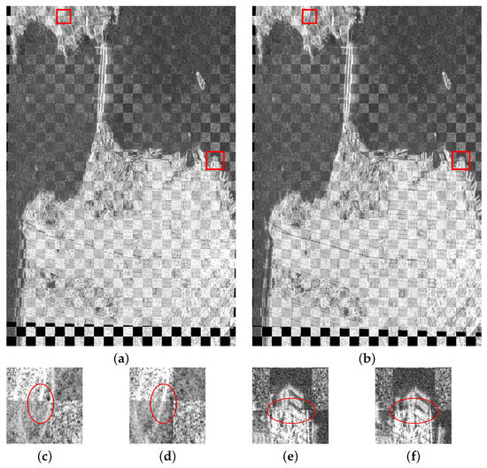
Figure 14.
Registration results of Image Pair 5: (a) Pre-registration results. (b) Fine registration results. (c) The first sub-image of pre-registration. (d) The first sub-image of fine registration. (e) The second sub-image of pre-registration. (f) The second sub-image of fine registration.
Table 6.
Comparison of SIFT, BFSIFT, SAR-SIFT, SAR-SIFT-Layer, SAR-SIFT-ISPCC, I-SAR-SIFT, SAR-SIFT-SWT, and the pre-registration and fine registration stages of the proposed method. (* indicates matching failure.)
The ENL values of the five image pairs range from 3 to 7, covering typical SAR image scenarios with moderate noise intensity (approximately 3–4) and relatively low noise intensity (approximately 5–6). In particular, the sensed images in Image Pair 2 and Image Pair 4 exhibit ENL values below 4, indicating significant speckle noise interference and belonging to relatively high-noise images. In contrast, the ENL values of Image Pair 3 and Image Pair 5 both exceed 5, classifying them as relatively low-noise images. Despite different levels of noise interference, the proposed method demonstrates good registration performance across all image pairs, especially achieving high-quality matching results in low-ENL images, which further verifies the robustness and adaptability of the method in high-noise environments.
The proposed method in this paper is compared with SIFT, BFSIFT, SAR-SIFT, SAR-SIFT-Layer, SAR-SIFT-ISPCC, I-SAR-SIFT, and SAR-SIFT-SWT. The SAR-SIFT-Layer method refers to a layer-by-layer registration strategy that constructs a multilevel image pyramid. It performs SAR-SIFT feature extraction and matching from low to high resolution layer by layer, using the transformation matrix obtained at each layer as the initial registration estimate for the next layer to refine and optimize the result progressively. As shown in Table 6, the proposed method achieves better results in terms of the NMP and RMSE. The two-stage matching strategy enables the acquisition of a significantly higher NMP in the final stage, thereby enhancing the reliability of registration results. The RMSE values confirm that the proposed method exhibits the smallest pixel deviation among all compared approaches. In terms of running time, Image Pairs 2 and 5 require longer running times in the pre-registration stage. For Image Pair 2, this results from a higher NOI, while for Image Pair 5, the longer running time is attributed to its larger image dimensions, which generate more extracted feature points. In the fine registration stage, Image Pairs 4 and 5 take longer due to the necessary local corrections in terrain-undulated areas. Specifically, Image Pair 4 involves corrections across six regions, leading to a runtime of 69.35 s, while Image Pair 5 requires corrections in a single region, resulting in a shorter runtime of 45.78 s.
It is noteworthy that SAR-SIFT exhibits better stability than the SIFT method. Although its RMSE for Image Pair 1 is 3.12, higher than SIFT’s 2.31, the RMSE values for Image Pairs 2, 4, and 5 are lower than those of the SIFT method. For the BFSIFT and SIFT methods, BFSIFT outperforms SIFT in both running time and RMSE. In terms of matching pairs, BFSIFT performs similarly to SIFT for Image Pairs 1, 2, and 4, but significantly worse for Image Pair 5. Image Pair 5, except for coastal edges, lacks distinct internal land edge information. As BFSIFT replaces the Gaussian filter with a bilateral filter, it is more sensitive to edge information, leading to a reduction in matching pairs. For Image Pair 3, experimental results show that at the original resolution, SAR-SIFT fails to achieve reliable matching due to obvious image deformation. After downsampling, 7 matching pairs are successfully generated in the pre-registration stage, providing a basic alignment for fine registration. This result indicates that the combination of downsampling and iterative strategies can improve the robustness of SAR-SIFT in cross-resolution images. For the I-SAR-SIFT method, although it achieves more matching pairs than SAR-SIFT, its RMSE performance is worse. This is because the multiplicative noise in SAR images causes deviations in the extracted feature points. Additionally, despite being a two-stage matching method, I-SAR-SIFT employs a block-based matching approach. When a mismatched pair within an image block is not removed, it disrupts the global registration results. Furthermore, the two-stage process makes I-SAR-SIFT significantly longer in running time than other methods. Nevertheless, compared with SIFT, BFSIFT, SAR-SIFT and SAR-SIFT-SWT, I-SAR-SIFT remains a more robust method, as it can achieve relatively accurate registration even when the other three methods fail for Image Pair 3. The SAR-SIFT-Layer method demonstrates better robustness compared with the SAR-SIFT method, particularly achieving effective matching in Image Pair 3. However, it still suffers from instability in registration accuracy and time overhead. This method relies on the matching accuracy of the pyramid’s top layer. When significant errors exist in the low-resolution layer, the results of high-resolution layers are prone to being affected, as evidenced by the unstable performance in Image Pairs 2 and 5. Theoretically, due to its hierarchical propagation mechanism, the SAR-SIFT-Layer should exhibit lower efficiency than the SAR-SIFT method. Nevertheless, in Image Pairs 1 and 5, SAR-SIFT-Layer shows superior efficiency. This is attributed to the significant reduction in the number of feature points extracted from the transformed image, which greatly influences experimental efficiency. The SAR-SIFT-ISPCC method demonstrates favorable performance in certain images (e.g., Image Pairs 1 and 3). However, in Image Pair 2, significant deviations introduced during the downsampling process lead to degraded fine registration performance, with the RMSE reaching 4.16. Additionally, the method exhibits suboptimal performance in terrain-undulated regions (Image Pairs 4 and 5), with relatively high RMSE values. This indicates that its fine registration strategy still faces challenges in fully adapting to complex terrains. The SAR-SIFT-SWT method improves efficiency and accuracy in certain image pairs (e.g., Image Pairs 1 and 4), but still fails to achieve effective registration for Image Pair 3, demonstrating the inherent limitations of SAR-SIFT. Additionally, in Image Pair 5, due to fewer points being eliminated during the SWT optimization stage and the relatively high computational load of the SWT transformation itself, the overall running time increases from 81.19 s (SAR-SIFT) to 96.11 s.
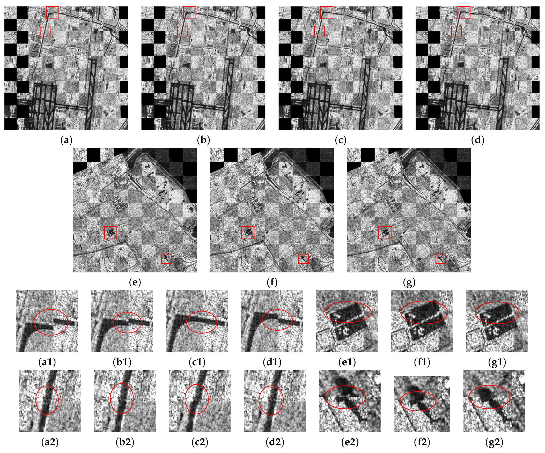
Taking Image Pairs 1 and 2 as examples, Figure 15 presents the registration results of SIFT, BFSIFT, SAR-SIFT, and I-SAR-SIFT for Image Pair 1, as well as the registration results of SAR-SIFT-Layer, SAR-SIFT-ISPCC, and SAR-SIFT-SWT for Image Pair 2. Here, (a–g) represent global registration results, while (a1–g1) and (a2–g2) show the registration results of the first and second sub-images, respectively. These correspond to the registration results in Figure 10 and Figure 11. In Figure 15, although (a2), (b2), (c1), (d2), (e1), (f1), and (g1) show favorable registration results, significant deviations remain in other sub-images. In Figure 10, (e) exhibits favorable registration results, (c) has significant deviations, while both (d) and (f) show good registration performance. In Figure 11, (c) and (e) has significant deviations, while both (d) and (f) show good registration performance. This is because some regions lack sufficient matching pairs, leading to significant errors in global registration that rely on local matching pairs. Overall, compared with the other seven methods, the proposed method provides the highest NMP, the smallest RMSE, and relatively low running time across the five image pairs.
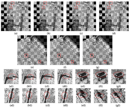
Figure 15.
The registration results of Image Pairs 1 and 2: (a–d) The registration results of SIFT, BFSIFT, SAR-SIFT, and I-SAR-SIFT for Image Pair 1. (e–g) The registration results of SAR-SIFT-Layer, SAR-SIFT-ISPCC, and SAR-SIFT-SWT for Image Pair 2. (a1–g1) The first sub-images of the corresponding image. (a2–g2) The second sub-images of the corresponding image.
4. Discussion
By fully leveraging the complementary advantages of feature-based and template-based matching methods, this paper proposes a robust and efficient SAR image registration method that integrates SAR-SIFT with template matching, coupled with an adaptive local stretching transformation. The method employs iterative optimization to refine the pre-registration results in the pre-registration stage, introduces a new similarity measure in the fine registration stage to achieve accurate registration in flat terrain areas, and combines adaptive local stretching transformation to handle the transformation in terrain-undulated areas. Experimental results demonstrate that this approach significantly enhances registration performance in complex terrains and exhibits strong generalization ability across diverse imaging conditions, including different SAR sensors, resolutions, and scene complexities.
When applying the SAR-SIFT method to downsampled SAR images for accelerating the pre-registration process, resolution reduction often leads to fewer and less distinctive feature points due to the loss of fine structural details. When these sparse keypoints are mapped back to the original image dimensions, they tend to generate significant localization errors because the spatial accuracy of matched points is compromised. This mismatch is particularly pronounced in complex terrain regions, where subtle structural variations are crucial for accurate alignment. To address this limitation, an iterative affine transformation update strategy is introduced, where the transformation matrix is continuously optimized until it reaches a stable convergence state. This iterative correction not only compensates for the deviation caused by downsampling but also enhances the robustness of the overall matching process. As demonstrated in the experimental results of Section 3.3, the iterative optimization approach significantly enhances registration quality, particularly in cases of poor initial alignment.
In the fine registration stage, relying solely on spatial or frequency domain information often fails to fully utilize the structural and textural features of SAR images. To address this limitation, a new similarity measure is proposed, which combines the phase congruency from the frequency domain and the gradient information from the spatial domain. As demonstrated in the experimental results of Section 3.4, the proposed measure outperforms traditional methods, including NCC, phase congruency, and gradient-based similarity measures in edge-rich regions.
In SAR image registration, significant topographic relief often introduces complex local geometric transformations that cannot be adequately modeled using global transformations alone. Relying solely on global affine models frequently results in local misalignments in terrain-undulated areas, leading to reduced registration accuracy and spatial inconsistencies. To address this limitation, an adaptive local stretching transformation is introduced following the template matching stage. This method identifies regions affected by topographic relief through local registration and applies adaptive stretching correction, without requiring external terrain data such as digital elevation models (DEMs). Experimental results on images with significant topographic relief, as presented in Section 3.5, show that the proposed stretching strategy effectively compensates for terrain-induced geometric deformations. Compared with traditional global models, the proposed method provides targeted correction for terrain-undulated regions, leading to improved registration accuracy in these areas and enhancing the overall registration performance of the entire image.
The two-stage design enables the proposed method to exhibit high precision at the expense of computational efficiency, making it more suitable for scenarios requiring high precision but low real-time performance (such as fine deformation analysis after disasters). This is particularly evident in Image Pairs 4 and 5, where transformations in terrain-undulated areas are time-consuming. This paper focuses on the theoretical innovations of the registration algorithm, including the two-stage framework and adaptive local stretching transformation. However, it has limitations in automation and efficiency, which are critical transition links from algorithm research to engineering applications. One of the future research directions is parallelization optimization, including accelerating operations such as feature extraction and template matching after block processing via GPU parallel computing, and exploring more efficient feature representations to reduce the computational load of the current PCGCC in calculating the fused features of frequency-domain phase congruency and spatial-domain gradients while maintaining precision. Another future research direction is multimodal remote sensing registration. The current method is primarily designed for high-precision registration of single-modal SAR data, especially in complex terrain areas, whereas optical-SAR or multiband SAR registration involves cross-modal radiation differences (such as the nonlinear relationship between optical intensity and SAR backscatter coefficient) and geometric distortion differences (such as the model differences between optical perspective projection and SAR slant-range projection), requiring additional solutions for challenges such as feature space alignment and cross-domain similarity measure.
5. Conclusions
In this paper, a robust and efficient SAR image registration method is proposed by combining SAR-SIFT and template matching, while accounting for local deformations caused by topographic relief. The proposed method consists of two stages: pre-registration and fine registration. In the pre-registration stage, images are downsampled, and the SAR-SIFT method is employed to extract and match feature points. The sensed image is initially aligned through affine transformation to obtain the pre-registered image. In this stage, the transformation model is iteratively optimized until the pre-registered image stabilizes, thereby mitigating potential large registration errors in the initial alignment. In the fine registration stage, a block-based strategy is adopted to ensure uniform distribution of feature points across the entire image. Additionally, a new similarity measure is proposed by combining the edge information from both the frequency domain and the spatial domain. Comparative experiments with image intensity-based NCC, frequency-domain phase congruency, and spatial-domain gradient methods demonstrate the effectiveness of the proposed similarity measure. Finally, to address local deformation caused by the topographic relief, an adaptive local stretching transformation is introduced to perform local correction on undulating regions. Experimental results show that the proposed method achieves accurate registration in terrain-undulated areas without relying on additional information (e.g., DEM). While the current method exhibits satisfactory performance, its computational efficiency in highly undulated terrains requires further improvement, which is an important direction for future research.
Author Contributions
Conceptualization, S.L. and X.D.; methodology, S.L.; software, S.L. and Y.C.; validation, S.L. and X.D.; formal analysis, C.L.; investigation, Y.C.; resources, C.L.; data curation, Y.C.; writing—original draft preparation, S.L.; writing—review and editing, C.L.; visualization, S.L.; supervision, C.L.; project administration, X.D. and C.L.; funding acquisition, X.D. and C.L. All authors have read and agreed to the published version of the manuscript.
Funding
This work was supported in part by Aeronautical Science Foundation of China (20240020053004), in part by the National Natural Science Foundation of China (NSFC) (Nos. 62101456 and 62171023), in part by the 2022 Suzhou Innovation and Entrepreneurship Leading Talents Program (Young Innovative Leading Talents) under Grant ZXL2022459, in part by the Basic Research Programs of Taicang under Grant TC2024JC12.
Institutional Review Board Statement
Not applicable.
Informed Consent Statement
Not applicable.
Data Availability Statement
Please contact Shichong Liu (liushichong@mail.nwpu.edu.cn) for access to the data.
Conflicts of Interest
The authors declare that there are no conflicts of interest regarding the publication of this paper.
References
- Li, Z.; Jia, Z.; Yang, J.; Kasabov, N. A method to improve the accuracy of SAR image change detection by using an image enhancement method. ISPRS J. Photogramm. Remote Sens. 2020, 163, 137–151. [Google Scholar] [CrossRef]
- Jiang, W.; Sun, Y.; Lei, L.; Kuang, G.; Ji, K. Change detection of multisource remote sensing images: A review. Int. J. Digit. Earth 2024, 17, 2398051. [Google Scholar] [CrossRef]
- Quan, Y.; Tong, Y.; Feng, W.; Dauphin, G.; Huang, W.; Xing, M. A novel image fusion method of multi-spectral and sar images for land cover classification. Remote Sens. 2020, 12, 3801. [Google Scholar] [CrossRef]
- Ye, Y.; Zhang, J.; Zhou, L.; Li, J.; Ren, X.; Fan, J. Optical and SAR image fusion based on complementary feature decomposition and visual saliency features. IEEE Trans. Geosci. Remote Sens. 2024, 62, 1–15. [Google Scholar] [CrossRef]
- Scaioni, M.; Marsella, M.; Crosetto, M.; Tornatore, V.; Wang, J. Geodetic and remote-sensing sensors for dam deformation monitoring. Sensors 2018, 18, 3682. [Google Scholar] [CrossRef]
- Guo, S.; Zuo, X.; Wu, W.; Yang, X.; Zhang, J.; Li, Y.; Huang, C.; Bu, J.; Zhu, S. Mitigation of tropospheric delay induced errors in TS-InSAR ground deformation monitoring. Int. J. Digit. Earth 2024, 17, 2316107. [Google Scholar] [CrossRef]
- Zitova, B.; Flusser, J. Image registration methods: A survey. Image Vis. Comput. 2003, 21, 977–1000. [Google Scholar] [CrossRef]
- Lin, Y.; Gao, Y.; Wang, Y. An improved sum of squared difference algorithm for automated distance measurement. Front. Phys. 2021, 9, 737336. [Google Scholar] [CrossRef]
- Mahmood, A.; Khan, S. Correlation-coefficient-based fast template matching through partial elimination. IEEE Trans. Image Process. 2011, 21, 2099–2108. [Google Scholar] [CrossRef]
- Viola, P.; Wells, W.M., III. Alignment by maximization of mutual information. Int. J. Comput. Vis. 1997, 24, 137–154. [Google Scholar] [CrossRef]
- Kovesi, P. Image features from phase congruency. Videre J. Comput. Vis. Res. 1999, 1, 1–26. [Google Scholar]
- Bunting, P.; Labrosse, F.; Lucas, R. A multi-resolution area-based technique for automatic multi-modal image registration. Image Vis. Comput. 2010, 28, 1203–1219. [Google Scholar] [CrossRef]
- Lowe, D.G. Distinctive image features from scale-invariant keypoints. Int. J. Comput. Vis. 2004, 60, 91–110. [Google Scholar] [CrossRef]
- Schwind, P.; Suri, S.; Reinartz, P.; Siebert, A. Applicability of the SIFT operator to geometric SAR image registration. Int. J. Remote Sens. 2010, 31, 1959–1980. [Google Scholar] [CrossRef]
- Wang, S.; You, H.; Fu, K. BFSIFT: A novel method to find feature matches for SAR image registration. IEEE Geosci. Remote Sens. Lett. 2011, 9, 649–653. [Google Scholar] [CrossRef]
- Wang, F.; You, H.; Fu, X. Adapted anisotropic Gaussian SIFT matching strategy for SAR registration. IEEE Geosci. Remote Sens. Lett. 2014, 12, 160–164. [Google Scholar] [CrossRef]
- Fan, J.; Wu, Y.; Wang, F.; Zhang, Q.; Liao, G.; Li, M. SAR image registration using phase congruency and nonlinear diffusion-based SIFT. IEEE Geosci. Remote Sens. Lett. 2014, 12, 562–566. [Google Scholar]
- Dellinger, F.; Delon, J.; Gousseau, Y.; Michel, J.; Tupin, F. SAR-SIFT: A SIFT-like algorithm for SAR images. IEEE Trans. Geosci. Remote Sens. 2014, 53, 453–466. [Google Scholar] [CrossRef]
- Wang, B.; Zhang, J.; Lu, L.; Huang, G.; Zhao, Z. A uniform SIFT-like algorithm for SAR image registration. IEEE Geosci. Remote Sens. Lett. 2015, 12, 1426–1430. [Google Scholar] [CrossRef]
- Liu, F.; Bi, F.; Chen, L.; Shi, H.; Liu, W. Feature-area optimization: A novel SAR image registration method. IEEE Geosci. Remote Sens. Lett. 2016, 13, 242–246. [Google Scholar] [CrossRef]
- Li, Y.; Stevenson, R. Incorporating global information in feature-based multimodal image registration. J. Electron. Imaging 2014, 23, 023013. [Google Scholar] [CrossRef]
- Gong, M.; Zhao, S.; Jiao, L.; Tian, D.; Wang, S. A novel coarse-to-fine scheme for automatic image registration based on SIFT and mutual information. IEEE Trans. Geosci. Remote Sens. 2013, 52, 4328–4338. [Google Scholar] [CrossRef]
- Ye, Y.; Shan, J. A local descriptor based registration method for multispectral remote sensing images with non-linear intensity differences. ISPRS J. Photogramm. Remote Sens. 2014, 90, 83–95. [Google Scholar] [CrossRef]
- Xiang, Y.; Wang, F.; You, H. An automatic and novel SAR image registration algorithm: A case study of the Chinese GF-3 satellite. Sensors 2018, 18, 672. [Google Scholar] [CrossRef]
- Paul, S.; Pati, U.C. SAR image registration using an improved SAR-SIFT algorithm and Delaunay-triangulation-based local matching. IEEE J. Sel. Top. Appl. Earth Obs. Remote Sens. 2019, 12, 2958–2966. [Google Scholar] [CrossRef]
- Wang, M.; Zhang, J.; Deng, K.; Hua, F. Combining optimized SAR-SIFT features and RD model for multisource SAR image registration. IEEE Trans. Geosci. Remote Sens. 2021, 60, 1–16. [Google Scholar] [CrossRef]
- Chen, S.; Zhong, S.; Xue, B.; Li, X.; Zhao, L.; Chang, C.I. Iterative scale-invariant feature transform for remote sensing image registration. IEEE Trans. Geosci. Remote Sens. 2020, 59, 3244–3265. [Google Scholar] [CrossRef]
- Venkatesh, S.; Owens, R. An Energy Feature Detection Scheme. IEEE Trans. Pattern Anal. Mach. Intell. 1989, 11, 358–367. [Google Scholar]


Disclaimer/Publisher’s Note: The statements, opinions and data contained in all publications are solely those of the individual author(s) and contributor(s) and not of MDPI and/or the editor(s). MDPI and/or the editor(s) disclaim responsibility for any injury to people or property resulting from any ideas, methods, instructions or products referred to in the content. |
© 2025 by the authors. Licensee MDPI, Basel, Switzerland. This article is an open access article distributed under the terms and conditions of the Creative Commons Attribution (CC BY) license (https://creativecommons.org/licenses/by/4.0/).