Abstract
This research discusses the application of Sentinel satellite data for monitoring air pollution in port areas. The Scopus and Web of Science databases were comprehensively analysed to identify relevant peer-reviewed literature and assess research publications. The systematic literature review was conducted using the PRISMA methodology for inclusion and exclusion criteria. A total of 519 articles were identified from which 70 relevant articles were finally selected and discussed in detail for their relevancy to the maritime environment. Sentinel-5P was found to have several use cases in the literature that are useful for measuring maritime air pollution, while Sentinel 1 and 2 were mainly used for other applications like oil spills and water quality, respectively. Although aerial surveys, like those conducted using unmanned aerial vehicles (UAVs), offer more precise estimates of greenhouse gases (GHGs), they are only useful for certain applications because the technology is costly and impractical for daily monitoring. Satellite-based sensors are the state of the art for obtaining remote observations of emissions in open sea. Sentinel-5P measurements offer daily data for air quality monitoring, which supports ground surveys to identify and penalize major emission sources and consequently support environmental management in accordance with contemporary policies. Pollutant concentration levels for the maritime sector can be analysed both spatially and temporally using Sentinel-5P data. In the future, addressing the limitations of the Sentinel-5P data, such as underestimation and source separation, could improve air pollution assessments.
1. Introduction
The Sentinel satellites are the constellation of satellites operated by the European Space Agency (ESA) under its Copernicus program [1]. Sentinel-1 and Sentinel-2, launched on 3 April 2014 and 23 June 2015, respectively, have applications for maritime surveillance, mapping sea ice and oil spills, responding to natural disasters and classifying land cover [2]. For atmospheric monitoring, the Sentinel-5 Precursor, launched on 13 October 2017 [3], carries the Troposphere Monitoring Instrument (TROPOMI), specifically designed to measure atmospheric pollutants in the troposphere [4,5]. Sentinel-5P provides state-of-the-art air pollutant data with global coverage. It has a temporal resolution of about 1 day while it has four spectral bands: UV, visible, near-infrared, and shortwave with bandwidths of 270–320 nanometers (nm), 310–500 nm, 675–775 nm, and 2305–2385 nm, respectively. The original spatial resolution of Sentinel-5P data was 7 × 3.5 km square (km2), which was improved to 5.5 × 3.5 km2 in 2019. The Sentinel programme’s open data policy has enabled researchers to develop innovative methods for maritime and atmospheric monitoring applications [6]. Ship monitoring systems mainly consist of two types of sensors, on-board and remote sensors, with remote sensors consisting of ground-based radar sensors and satellite sensors [7].
Satellite sensors are one of the most important data sources for obtaining unbiased observations from ships in the open ocean [8]. Sensors such as TROPOMI offer unparalleled data compared to surface monitoring stations. Using satellite data for emission monitoring is an economical way to enhance environmental performance and increase public access to emission information [9]. Therefore, the integration of the Sentinel satellites in maritime and atmospheric monitoring capabilities is an important asset for assessing the impact of ship emissions on air quality, contributing to the management and mitigation of maritime pollution.
Complementary atmospheric monitoring satellites that also provide measurements for air pollutant concentrations include National Aeronautics and Space Administration (NASA) Earth Observation System—AURA (EOS-CH1), ESA Greenhouse Gases Observing Satellite (GOSAT), ESA Meteorological Operational Satellite Program of Europe (MetOp), Suomi National Polar-orbiting Partnership Satellite (Suomi NPP), Geostationary Korea Multi-Purpose Satellite—2B (GEO-KOMPSAT-2B), and NASA Intelsat 40 epic (IS-40e). Access to the data from these remote sensing satellites is also free for users. Using data from these multiple sources ensures consistency and improves temporal coverage, accuracy, reliance, and cross-validation capability. The Ozone Monitoring Instrument (OMI), onboard the AURA EOS-CH1 satellite, has provided daily ozone measurements since 2004 [10]. It is also used for tracking shipping emissions and it is an important alternative data source to Sentinel-5P. It provides data related to ozone (), nitrogen dioxide (), sulphur dioxide (), formaldehyde (HCHO), and aerosols [10]. It has a lower spatial resolution than Sentinel-5P but it provides data over a longer period of time. The Infrared Atmospheric Sounding Interferometer (IASI) aboard the MetOp series of satellites (operated by EUMETSAT) is a powerful instrument for atmospheric composition monitoring, including carbon monoxide (), , ammonia (), , , methane (), and carbon dioxide () air pollutants [11]. The Ozone Mapping and Profiler Suite (OMPS) on board the Suomi NPP satellite, launched in 2011, detects aerosols and tracks the total amount of ozone from the surface to the top of the atmosphere [12]. ESA, in 2002, launched Envisat, fitted with the Scanning Imaging Absorption Spectrometer for Atmospheric Cartography (SCIAMACHY) for atmospheric gas monitoring, including , , , , and [13]. The Japanese Earth observation satellites, GOSAT and its successor GOSAT-2, launched in 2009 and 2018, respectively, provide and measurements through the Thermal and Near-Infrared Sensor for Carbon Observations (TENSO) spectrometer onboard [14]. These satellites have shared polar sun-synchronous orbits (except GEO-KOMPSAT-2B and IS-40e), allowing for synergistic observations, while their overlapping measurement capabilities allow cross-validation, continuity, and robustness of global atmospheric monitoring data.
The Tropospheric Emissions Monitoring of Pollution (TEMPO) and Geostationary Environment Monitoring Spectrometer (GEMS) are emerging remote sensing satellites in this field in addition to Sentinel-5. TEMPO is a satellite launched by NASA on 7 April 2023, specifically to monitor air pollution over North America from a geostationary orbit [15]. TEMPO is the only instrument currently that offers a higher spatial resolution than TROPOMI. It monitors pollutants including , , , HCHO, formaldehyde, glyoxal, and aerosols. GEMS is a satellite launched by South Korea on 19 February 2020, to monitor air pollutants over East Asia from a geostationary orbit [16]. It is the first of its kind in the world to operate from a geostationary orbit solely for air pollutant (, , , HCHO, , aerosol) monitoring [17]. While these two sensors provide high-resolution atmospheric pollution data for specific regions, they do not offer coverage beyond their designated observation areas.
The maritime environment facilitates over 80% of global trade, contributing to economic growth, employment, investment, and government revenue while ensuring national and regional security [18]. It is the cheapest means of bulk mass transportation; consequently, the maritime sector is given substantial emphasis in national development planning and policy frameworks [6,19]. The International Maritime Organization (IMO) established a rule in 2000 mandating the installation of automatic identification systems (AISs) on all ships [20]. According to these rules, every ship involved in commercial maritime operations must transmit an AIS signal with vital details such as the ship’s identification, type, position, course, and speed. According to global estimates, the maritime shipping industry produces roughly one billion metric tons of each year [21]. Maritime transportation is responsible for approximately 54% of and of emissions [22]. In European coastal areas it has been a contributor to air quality degradation and climate change [23,24]. The European Union (EU) action plan mandates its ports to monitor and report emissions, with the aim of reducing emissions from the maritime sector and supporting the International Maritime Organization’s (IMO’s) energy efficiency strategy. This effort is focused on adaption of existing vessels to comply with emission control standards, implementing technological upgrades, developing low-emission fuels, and establishing the necessary infrastructure [25].
The concentration in particular was found to be higher along international shipping routes [22]. In the European Union, around 90% of trade is through shipping [22]. Emissions from the maritime sector represent a significant source of air pollution in harbour regions, with European harbours exhibiting the highest levels of and particulate matter (PM) 10 concentrations [26]. Shipping emissions contribute to increases in concentrations exceeding 20% in certain urban areas along Portugal’s west coast [26]. Communities are exposed to air pollution levels that represent a risk to their health, including the mortality rate from lung and cardiovascular cancers as well as early mortality from prolonged exposure to pollutants [27]. Given the magnitude of emissions and their impacts on public health and air quality, the use of advanced monitoring and spatial analysis technologies is increasingly essential to support mitigation policies and environmental management in the maritime sector.
The use of remote sensing and Geographical Information Systems (GISs) for maritime port management has increased in recent years [28,29]. Several studies have been conducted using Sentinel-5P data related to air pollution; however, there is a lack of discussion about maritime ports’ contribution. There is a notable absence of a comprehensive literature review that systematically synthesizes these efforts as none of the previous studies have discussed the contribution from the application of Sentinel data related to maritime air pollution collectively. This lack of consolidated discussion hampers a clear understanding of methodological trends, current advancements, and challenges faced. Consequently, there is a pressing need for a structured review to bridge this gap, offering researchers and policymakers a coherent overview of existing knowledge and guiding future research directions.
This review paper provides (1) a comprehensive foundation on the current state of maritime air pollution monitoring using Sentinel data; (2) a detailed systematic evaluation and bibliometric analysis of the available literature to improve knowledge of the application of Sentinel data in the maritime sector and the types of pollution caused by ships during maritime transportation; (3) a systematic evaluation of the strengths and limitations of the Sentinel satellites, particularly TROPOMI, in monitoring maritime air pollutants (, , , aerosols, and ); and (4) identification of potential avenues for future research to promote sustainability in the maritime port sector.
2. Materials and Methods
A systematic literature review (SLR) methodology was adopted for search, selection, and review of the articles. The SLR comprised a step-by-step approach for an objective identification of articles for review. The following paragraphs explain each step included in the methodology for the inclusion of articles.
There are several ways to identify literature related to the topic; however, not all are appropriate for a scientific review. The procedures adopted served as the foundation for the identification of records for the bibliometric analysis. The Web of Science and Scopus databases were searched specifically in this research. The two databases host high-quality, indexed, and peer-reviewed journals across multiple disciplines with a broad research coverage. Both databases have well-defined inclusion criteria which eliminate low-quality content.
To achieve a thorough review of the databases, precise keywords were chosen after a refining process. The initial search included articles, books, book chapters, conference papers, and reviews to ensure relevant peer-reviewed information. The search was restricted to studies from 2018 onward to achieve a focus on air quality applications following the launch of Sentinel-5P in October 2017. Table 1 shows the list of keywords used in the query for the document search in the databases.

Table 1.
Inclusion criteria in the databases.
A total of 519 articles were identified in the two databases. For further detailed scrutiny, the Preferred Reporting Items for Systematic Reviews and Meta-Analyses (PRISMA) framework was used. A total of 190 articles were excluded at this stage due to lack of access to full text, lack of relevance to the searched area, or for being in a language other than English. In this review, only English-language articles were included, given the language’s dominance in disseminating scientific knowledge globally [30,31]. Only nine articles were found in languages other than English, including seven in Russian, one in Chinese, and one in Persian. The remaining 329 articles were collectively examined using the VOSviewer software to examine the related topics, frequent terms, and existing trends through a visual analysis. The version of VOSviewer used was 1.6.20 [32]. The downloaded papers were managed in a folder and a bibtex file was used. The duplicate analysis was carried out using the Zotero 6.0.36 software [33]. Figure 1 presents the methodological flowchart for the study.
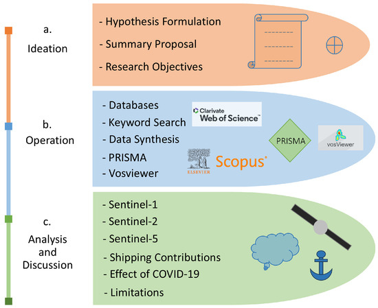
Figure 1.
Research methodology flowchart.
2.1. PRISMA
The PRISMA framework was adopted for the screening and eligibility stage [34]. After a collective analysis of the downloaded papers, the next step was to select the relevant papers for a more in-depth manual review. Figure 2 shows the inclusion and exclusion of the articles using the PRISMA framework.

Figure 2.
PRISMA methodology flowchart for article selection.
The total number of articles downloaded was 519. The downloaded papers were further scrutinized in three stages. After the first database refinement, the remaining 329 were considered for scrutiny and after passing through the three stages of screening, the number of remaining articles was 70.
The first stage involved eliminating papers based upon the following criteria: use of Sentinel data for ports, pollution, and the maritime environment. This stage involved reading the abstracts of the downloaded papers; from this stage 138 articles were eliminated.
The second stage included the categorization or labelling of articles into themes. This was achieved by having a full-text overview of the main topic being discussed. Ten articles were further screened for their lack of relevancy to our topic. Out of the total remaining papers for Sentinel-5P, thirty-three were on the topic of nitrogen oxides (), seven on , five on , three on carbon oxides (), two on sulphur oxides (), one on aerosol, and six on overall GHGs. Of the total of papers for Sentinel-2, only six papers discussed air pollution, and two of them were relevant to maritime studies. Forty-two articles were related to water quality, turbidity, and water pollution, while five articles were related to oil pollution. The Sentinel-1 papers were mainly related to oil spills. Out of fifty-one articles, forty-five were on the topic of oil spill detection while six were on air pollution. Finally, the articles on air pollution were reviewed. A comprehensive and rigorous analysis of the final selection of articles is presented in the Results and Discussion section.
2.2. VOSviewer
VOSviewer is a freely available software tool designed for creating maps to visualize bibliometric networks and data relationships [32]. It was employed to visualize and analyse the co-occurrence network of keywords using complete counting. Complete or total counting was preferred over binary counting, leading to a more profound identification of the central themes and their interconnections within the selected literature. A standard minimum threshold of 25 occurrences per term was applied during the analysis. From an initial pool of 8280 terms, 143 met this frequency criterion and were shortlisted for further examination. To refine the selection, VOSviewer calculated the relevance of each term, and using its default settings, the top 60% of the most relevant terms were chosen, yielding a final set of 85 terms for detailed analysis. This filtering process focused on the most significant and frequent terms, helping to identify patterns and core themes in the literature under review. Figure 3 shows the visualization made using the VOSviewer software.
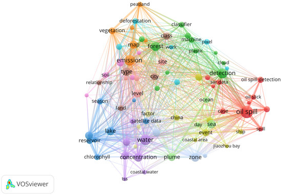
Figure 3.
Co-occurrence map showing frequently occurring terms using VOSviewer.
The shape in Figure 3 is roughly a triangle, which can be explained by there being three Sentinel satellites which are mainly designed for three different purposes. Therefore, the main applications can be generally divided into three categories.
3. Results and Discussion
In this section, the specific papers (70) with high relevancy to the maritime environment and ships are discussed in detail. Figure 4 displays the countries of the affiliations of the authors. Most authors were affiliated with institutes from the United States, followed by the United Kingdom and the Netherlands. The trend among the number of relevant articles published over time is increasing. The year 2023 had the largest number of published studies. Figure 5 shows the number of articles published each year, where blue dotted lines depict the overall trend in eight years while the orange line depicts the trend each year. There exists an increasing trend overall, while the trend among individual years is varying in the number of articles. While such maps, graphs, and their associated statistics inevitably carry some degree of bias, the distribution nonetheless provides an initial insight into the subject of discussion.

Figure 4.
Map with number of authors from different countries around the world for the selected articles.
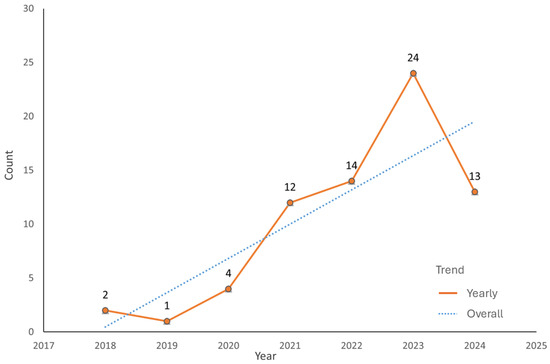
Figure 5.
Trend in number of articles published each year.
Table 2 shows the spread of the selected articles among journals. The articles were published in 36 unique journals, with the majority related to remote sensing, atmosphere, environment, and geosciences. Eleven journals published more than one article. Table 3 presents the distribution of the selected articles among the top eleven institutions, ranked by the number of publications. The National Aeronautics and Space Administration (NASA) had the largest number of articles followed by the Karlsruhe Institute of Technology (KIT) and the Royal Belgian Institute for Space Aeronomy (BIRA-IASB).
Table 2.
Distribution of articles in journals with at least two published articles.
Table 3.
Top eleven research institutions by number of articles.
3.1. Sentinel-1
The Sentinel-1 satellite is often used for ship detection but it is not optimal for air quality studies. Still, some insightful studies were found which are discussed further.
Christiani et al. [35] explored greenhouse gas (GHG) emissions monitoring using geospatial data and remote sensing. The geospatial data included climate, topography, and habitat variables, while the remote sensing data included Sentinel-1 and Sentinel-2 satellite data [35]. The methodologies can be extended to maritime emission mapping by fine-tuning machine learning models such as the MaxEnt model. Ports and shipping lanes can adopt these techniques to monitor and emissions, ensuring adherence to environmental standards.
While primarily focused on permafrost regions for emissions monitoring using Sentinel-1 and Sentinel-2 data, the adopted methodology can also be improved to track emissions from LNG-powered vessels and along key maritime routes [36]. In another study, synthetic-aperture radar (SAR) and multispectral data were used to map and emissions in icy regions as well [37]. These techniques have potential applications in maritime routes through polar regions, where shipping activities can cause and emissions. Monitoring these emissions can help regulate environmental impacts in sensitive ecosystems.
Spatial analysis of carbon emissions using Sentinel-1 data demonstrated its effectiveness in detecting emissions from large-scale environmental events like wild fires [38]. Similar techniques can be applied in maritime settings to monitor emissions caused by ship fire accidents and cargo handling operations.
The Sentinel-1 imagery was integrated with the Weather Research and Forecasting (WRF) model for checking offshore wind potential [39,40]. The model provides high-resolution data on wind speed, direction, and atmospheric conditions, supporting maritime applications such as optimizing ship routes. Ports can utilize these datasets for better operational planning and enhanced environmental compliance.
3.2. Sentinel-2
Sentinel-2 is not primarily used for air pollution mapping, although it is useful for the mapping of other types of pollution such as water contamination and solid waste detection. Some partially relevant studies are discussed in this section.
Sentinel-2 data was used to improve methane plume detection using the matched filter algorithm [41]. The algorithm was applied on Sentinel-2 time series for the Permian Basin area in the United States, Korpeje in Turkmenistan, and Hassi Messaoud in Algeria. It can be adopted to detect methane emissions from LNG-powered vessels and shipping corridors.
Sentinel-2 was also used to detect plumes from power plants and to estimate emissions from forest fires [42,43]. With the increase in spatial resolution, these methodologies can be also applied to ships to identify hotspots caused by vessel traffic and port equipment. These insights are valuable for regulatory compliance and improving air quality in maritime environments. This methodology can be adapted to estimate emissions due to maritime accidents.
The monitoring of particulate matter () through Sentinel-2 data offered insights into fine particulate pollution [44,45]. Near-real-time monitoring can aid in regulatory enforcement and pollution control.
A comprehensive analysis of human-induced transformations in pollution was performed for the Fatala River Basin, Guinea, Africa [46]. This study primarily used Sentinel-2 and Sentinel-5P data. The data was accessed through Google Earth Engine. Hazard classification and pollutant concentration mapping were presented for the catchment area of Fatala River Basin, showing the spatial distribution of anthropogenic pollution.
As of right now, there are no satellite measurements that can measure in the lower troposphere and are precise enough to be utilized to calculate fluxes between the surface and the atmosphere [47]. The MIN2OS instrument, expected to fly in 2031–2032, is going to be deployed on a platform operating in coordination with two additional platforms, Sentinel-2 and Metop-SG. A thermal infrared sensor will be used to overcome limitations, particularly the inability to effectively capture information in the lowermost troposphere.
3.3. Sentinel-5P
In the analysis of air pollution, the application of Sentinel-5P can be further categorized into different types of gaseous compounds including , , , and . is the main gas emitted from ships apart from . In our research, 39 out of 58 selected articles for Sentinel-5 discussed the contribution, with 33 specifically discussing only. Therefore, the main focus here is the application of Sentinel-5P for monitoring maritime emissions.
3.3.1. Nitrogen Dioxide ()
Using Sentinel-5P data for an analysis of the 29 major ports in the Mediterranean, Pseftogkas et al. [48] concluded that the observed 27% increase in average levels was attributable to the maritime sector. The sensitivity limits of TROPOMI to detect plumes from ships was analysed for establishing a minimum criterion of identifying the plume from a sea-going ship [49]. The minimum detectable length of a ship using Sentinel-5P was found to be 100–150 m.
Abdullah et al. [50] used Sentinel-5P to evaluate how Malaysia’s major port cities’ air quality was affected by maritime transportation, relating it to human and environmental health. levels at 11 ports were measured both before and after the COVID-19 pandemic to check the trend during the pandemic. The results indicated that maritime operations contribute to increased air pollution and emissions in Malaysia’s coastal areas. A strong correlation was found between ground data and the TROPOMI data [50,51]. Future recommendations emphasized enhancing the resilience of coastal ecosystems in the face of climate change.
On a European scale, the regions of the western British Isles, Northern Italy, and Central Europe have the highest levels [52]. Hotspots were observed in the biggest cities, such as Madrid, Barcelona, and Lisbon. One of the locations on Earth with the highest volume of ship traffic is the Strait of Gibraltar, which serves as a natural channel for communication between the Atlantic Ocean and the Mediterranean Sea. The study conducted by Adame et al. [52] analysed monthly trends and the frequency of pollution incidents, using in situ data to compare them with Sentinel-5P data. This analysis utilized hourly data collected over an extensive eleven-year period (2008–2019) from the El Arenosillo observatory, located in south-western Spain. Using the Sentinel-5P data, it was revealed that regions with elevated levels included the Guadalquivir Valley (moderate concentrations), the metropolitan area of Seville, the industrial sector of Huelva, and the Strait of Gibraltar along with the nearby areas the Gulf of Cadiz and the Alboran Sea [52]. Collectively, these areas represent a significant zone with high nitrogen dioxide levels. The yearly absolute maximums varied from 34.7 micrograms per cubic meter (µg m−3) in 2013 to 82.8 mg µg m−3 in 2015. The latter was the eleven-year period’s historical annual peak. Hourly readings were also analysed. These findings indicate that the European Air Quality Directive’s (Directive 2008/50/EC) hourly criterion, which has a value of 200 µg m−3, was not surpassed.
In 2021, stricter controls were implemented to limit () emissions from ships operating within the North and Baltic Seas [8]. Air quality station data and the TROPOMI satellite primarily report rather than . In situ surveys can be performed to provide a more detailed understanding, encompassing both NO and , revealing significant gradients. NO is particularly important near the emission source, while over time and with distance, NO is converted into , so that “aged” air pollution predominantly consists of . As a result, in cleaner Pacific air, the NO/ ratio tends to be close to zero [53]. Monitoring ship emissions in open-sea regions is uniquely reliant on satellite-based measurements, as no alternative instruments can provide similar coverage. The most advanced method currently available for large-scale estimation of ship-derived involves supervised machine learning techniques. These methods focus on segmenting ship plumes from Sentinel-5P satellite images [8].
The difficult data annotation and an inadequately sophisticated ship emission proxy limits the model’s application for ship compliance monitoring and validation. Applying a combination of machine learning models to TROPOMI satellite observations, a methodology was crafted for the automatic and scalable screening of possibly-non-compliant ships [54]. Image segmentation techniques can also be employed for identification of hotspots. Tropospheric data from the TROPOMI exhibited a strong correlation (r = 0.87) with surface measurements across both land and water in the New York Port area [55].
Wang et al. [56] investigated the spatiotemporal properties of in twelve ports across the globe and examined how significant shipping events affect marine atmospheric . Satellite data, emission inventories, meteorological data, and models such as the Long-Term Ozone Simulation-European Operational Smog (LOTOS-EUROS) chemical transport model were used. Marine atmospheric changes were analysed using the TROPOMI and the Chinese Environmental Traces Gases Monitoring Instrument (EMI), particularly during the global COVID-19 pandemic and growing geopolitical issues. For individual ships, a proxy was calculated using the formula in Equation (1). The same approach was adopted by Georgoulias et al. [20], as well as calculating emissions solely using the ship’s length and speed, which can be accessed via AIS data. The total daily emissions for any region can be determined by aggregating the emissions from all active ships within that region. Current regulations have decreased anthropogenic emissions, although this is not true for all ports [56]. levels in three Chinese coastal ports (Beibu Gulf, Ningbo-Zhoushan, and Lianyungang) was successfully lowered under the present emission control area (ECA) regulations [56]. This approach does not take into account other anthropogenic emissions like industrial operations at ports. With high-resolution satellite data, better estimations can be achieved. For future research, data from emission inventories and models can be combined with satellite data to gain more accurate results.
where L represents the ship’s length in meters, and U denotes its speed in meters per second (ms−1).
Petetin et al. [57] examined the variability of concentrations detected by TROPOMI (TrC-) over the Iberian Peninsula between 2018 and 2021. This study integrated ground-level air quality data, contributions from human activities, and natural emissions from soil, as well as complementary datasets such as ERA5. For observing emissions, an algorithm was developed in Python that requires the ERA5 reanalysis and TROPOMI level-2 data. The study also assessed the influence of cloud cover on the availability of TROPOMI data and analysed the distribution of TrC- measurements across the region [57]. Furthermore, the relationship between TrC- data and surface mixing ratios was investigated. The researchers also examined TrC- variability on weekly, monthly, and yearly scales. Spatial maps were used to depict various regions and key urban centres in the area, offering a detailed visualization of the findings. On average, TROPOMI TrC- observations are accessible on approximately 55–60% of the days across the Iberian Peninsula, with similar data availability in Spain and Portugal [57]. Murcia and Asturias region were found to have most and least availability of TROPOMI data, respectively. The lowest availability is observed in April and November (around 30–45%), moderate levels occur during the winter months (approximately 45–60%), and the highest availability is seen in summer (ranging from 70 to 80%). On the Iberian Peninsula, Madrid was found as the most significant pollution hotspot for tropospheric , with Barcelona following closely behind. Apart from urban areas, which usually have several surface monitoring stations, TROPOMI’s greatest potential lies in its observations over rural regions and seas.
TROPOMI was compared to the Ozone Monitoring Instrument (OMI) for ship emissions detection [58]. When assessing relatively small increases in pollution over dark European oceans, TROPOMI performs better than OMI [58]. The researchers also reported that black water appears white (high reflectance) in TROPOMI data when there is sun-glint, which significantly increases the effective scene albedo and decreases the scattering angle. The signal intensity from spectral fitting of columns along the average light path is raised by 20% to 30% over clear-sky shipping lanes due to this higher apparent scene reflectivity. Furthermore, under these circumstances, the marine boundary layer’s vertical sensitivity to increases by as much as 60%. Under sun-glint circumstances, plume-like structures of ship emissions can be seen in TROPOMI columns [20] Sun-glint situations are particularly useful for detecting small-scale emission sources over open seas that were previously invisible. By aligning the 3-h ship tracks preceding the Sentinel-5P flyover with the prevailing near-surface wind patterns, these structures line up with ship plumes [20].
Larger ships have the most noticeable plume formations. Larger ships, mostly crude oil tankers and container ships, are the source of most of the plume-like structures in tropospheric . Plumes caused by emissions from large individual ships and clusters of ships in close proximity can be detected in single-flyover TROPOMI/S5P tropospheric column data under favourable conditions like cloud-free skies, low wind speeds, and sun-glint [20].
The plumes produced by sea-going ships were automatically segmented using a supervised machine learning technique using Sentinel-5P data [59]. The XGBoost model performed the best out of the five machine learning models that were evaluated. This approach improved the average precision score by 20% and produced a correlation of 0.834 with a conceptually constructed emission proxy [59]. The automated monitoring of ship emissions using remote sensing data was improved by offering a reliable and effective method of tracking pollution.
Ship tracks hardly ever cross one another and most of the time follow the same shipping lanes [20]. Because of this, emissions frequently mix, making it more difficult to assign specific ships to tropospheric column readings. Ship tracks were identified by Pseftogkas et al. [60] using TROPOMI due to higher presence along those paths. The identified routes were from the Strait of Gibraltar to the Suez Canal [60] and from the Aegean Sea to the Bosporus Strait. observations close to coastlines are higher due to port operations and inland emissions, with the coasts of Barcelona and Valencia showing very noticeable columns.
Ship emissions are distinctly visible in most seas, particularly along heavily trafficked shipping routes [61]. A strong geographical correlation was observed between frequent shipping routes linking the Canary Islands and levels, especially in weekly averaged data [9]. Notable increases in concentrations were observed in the central areas of these primary shipping lanes, attaining levels of molecules . The researchers confirmed that the sensor’s cumulative signal over various time periods exhibits a spatial pattern that closely aligns with the vessel distribution in the Tenerife–Gran Canaria channel. The approach adopted by Kim et al. [62] showed an enhanced geographical correlation between the frequency of shipping activity and column clusters in the Mediterranean and Red Sea and Indian Ocean. Furthermore, a temporal correlation was found between column levels throughout shipping routes. Extensive testing and validation using data gathered from various places and time periods proved the reproducibility of the methodology [62]. It was anticipated that this method would act as a prototype for detecting and differentiating anthropogenic maritime emissions from background sources. Rather than estimating absolute emissions, the study concentrated on finding relative hotspots and trends in concentrations along shipping routes. In order to confirm that the clustering appropriately reflected shipping patterns and economic trends, the approach’s validity was checked by contrasting the results with publicly available ship track count estimates and a global logistics index. These results are consistent with the Copernicus Atmospheric Monitoring Service (CAMS) globally validated inventories for seafaring vessels, that showed comparatively higher emissions in the summer than in the winter [62]. columns are often greater in the winter and decrease in the summer, though another study found that pollution levels are higher on the hottest days [60,63]. The suggested approach provides a monitoring tool to track relative changes in aggregate emission levels within any zone, making it useful for port authorities or inspectorates.
Riess et al. [64] used an aircraft from the Royal Belgian Institute of Natural Sciences that was fitted with a sniffer sensor system to measure , , and over the contaminated parts of the North Sea, which included important shipping lanes, industrial areas, and populated coastal regions. Three horizontal scans and ten spiral flights were made to acquire vertical profiles in the lowest 1.5 km of the troposphere. The aircraft successfully captured ship plumes and pollution throughout the North Sea by flying as low as 30 m above the sea surface. The vertical columns for CAMS and LOTOS-EUROS were abnormally higher than the aircraft-based measurements. Using its capabilities to measure over the water, the Belgian Coast Guard regularly uses this aircraft for ship emissions compliance monitoring [64].
Satellite-derived data can be used to detect oil and natural gas (ONG) offshore activities though they are not able to fully capture the extent of ambient fluctuation in areas with a large number of ONG systems [65]. Additionally, TROPOMI is quite good at detecting emissions from airports, shipping activities, and high-traffic areas, as well as collecting fine-scale spatial fluctuations in urban areas. Previous satellite instruments have not achieved this degree of precision, especially during shorter time periods of up to one year [63].
CAMS has established an operational system for regional air quality forecasting, using an ensemble of European models with high resolution: [66]. Overall, there is a good agreement between the values from TROPOMI and the forecasts and analysis from the CAMS AQ models. A number of comparison points, however, draw attention to inherent uncertainties in the TROPOMI and CAMS models, pointing to areas that require more improvement [20,66]. More precise forecasts of present and future climatic conditions may result from the inclusion of updated ship emissions in climate modelling studies [20]. A general agreement between the Collaborative Column Carbon Observing Network (COCCON) and satellite-derived products was found when the COCCON spectrometers were compared with satellite data such as TROPOMI and CAMS [67]. However, because of atmospheric light scattering and the low albedo of the sea surface, satellites have difficulty detecting air pollution close to the sea surface.
On 4 August 2020, a huge explosion in Lebanon’s Beirut seaport killed more than 200 people and severely damaged other nearby structures. A supposition existed that the explosion, which was caused by ammonium nitrate (AN), released a lot of into the atmosphere, which might have seriously endangered the health of people in Beirut and the neighbouring areas [68]. Investigating the spatiotemporal distribution of during and after the incident and comparing it to the usual daily background emissions from Beirut’s ship and vehicle traffic was important in determining the significance of the explosion’s emissions. Farahat et al. [68] examined concentrations in the atmosphere prior to, during, and following the Beirut explosion using Sentinel-5P TROPOMI data. According to the analysis, concentrations over the city increased to approximately 1.8 mol/ within twenty-four hours after the explosion and then progressively decreased over the course of four days. Notably, concentrations rose to 4.3 mol/ seven days before the blast (on 28 July 2020). This was mainly caused by car emissions and ships travelling close to the Beirut seaport from July 20 to 26. These results suggested that levels increased temporarily as a result of the Beirut explosion. The release of gas from ammonium nitrate (AN) explosions was found to have caused atmospheric alterations that were seen in Beirut after the disaster and the suppositions proved to be true [68].
A study monitoring air pollutants in Guayaquil, Ecuador, was conducted using Sentinel data combined with interpolation methods [69]. The mid-sized port city lacks a permanent air quality monitoring network, making it challenging to assess air quality from ground measurements directly. To address the pixel-size constraint of Sentinel data, interpolation techniques were applied. The advanced Bayesian kriging (ABK) technique delivered the highest precision (). The strategy adopted in this research supports monitoring air quality in areas without fixed observation systems, as smaller pixel dimensions provide a more refined distribution of pollutants.
All commercial sea-going vessels have been required to carry an AIS transponder since 2002 in order to ensure that their identification, type, position, course, and speed are tracked. Future plans call for greater regulation of air pollution from maritime operations as the Mediterranean Sea was designated as an emission control area (ECA) in 2025 [48].
Table 4 categorizes articles according their subject of discussion. The datasets used to analyse the corresponding pollutants are also highlighted in the table. A few studies fall into more than one subject category; therefore, they are suggested for more than one subject. A survey of data and code availability was performed for the Sentinel-5P articles on . Table 5 presents the results, showing data availability for most of the articles. Since Sentinel-5P data, which is already open-access, was used in these articles, the authors have opted to make the processed data publicly available for the majority of the studies. Six studies were found for which code is available; these can be reproduced more easily.
Table 4.
Categorization of articles relevant to maritime pollution in section.
Table 5.
Survey of data and code availability for articles in section.
3.3.2. Sulphur Dioxide ()
is a hazardous air pollutant because it is an extremely harmful material for both human health and the environment, due to its strong influence on morbidity and mortality rates [80]. On the positive side, through a ten-year analysis, Saliba et al. [3] came to the conclusion that emissions of and are gradually declining over time. The Giordan Lighthouse in Malta reports ten years of air quality observations, identifying two main sources of sulphur emissions: shipping and Mount Etna’s volcanic activity [3].
The authors monitored ship emissions, particularly examining the marine environment surrounding Malta, in order to determine how much shipping contributes to local air pollution [3]. The orthorectified offline data product (Level 3), accessed through Google Earth Engine, was used for quantification [3]. Atmospheric phenomena are innately spatial, therefore spatial regression models were compared in order to take into account spatial autocorrelation. A high level of clustering was indicated in concentrations measured by TROPOMI. This approach can be useful for measuring emissions through ships.
Schmidt et al. [81] analysed major emission sources of , with a focus on the US metal industry, to highlight the issue of greenwashing. Greenwashing is the false portrayal of companies as environmentally friendly. A spatial regression analysis was used to examine the connection between concentrations and the US metal industry using TROPOMI data and a database with companies’ data. Web text data was also considered, categorizing businesses according to their websites to show how they present themselves on the subject of sustainability. The approach, used primarily for the metal industry, could be applied to the maritime sector.
3.3.3. Ozone ()
The Ozone Water–Land Environmental Transition Study (OWLETS) was a prototype methodology for examining the relationships between emissions, contaminants, and the intricate coastline [82]. OWLETS offers a unique dataset in which it is possible to identify pollution episodes in combination with the operational air quality forecasts from the NOAA National Air Quality Forecast Capability (NAQFC). The observations showed higher levels over water (both at the surface and above) compared to land, which usually happens in the afternoon when levels are at their first peak, indicating that the variability in pollution was caused by ship emissions. In areas where shipping channels were present over water, observations revealed a significant spatial variability in and concentrations [82]. It is important to describe air quality, validate forecasts, and assess satellite products in light of stricter pollution regulations.
The physiochemical mechanisms that are linked to increased ozone were studied using an inversion framework [73]. The findings presented previously unmeasured features of changes in ozone and its precursor emissions during the lockdown in 2020.
In California, observations from a smog chamber were analysed for daily and seasonal variations and direct ozone measurements were analysed with the TROPOMI HCHO/ ratios [83]. sensitivity in most of California follows a cyclical pattern similar to Sacramento, according to monthly averaged TROPOMI observations [83].
In Texas, an evaluation of emissions and their effect on ozone revealed that lightning contributes 8% of in the air [84]. TROPOMI is more sensitive to the upper troposphere. Air quality over the United States is measured by the Tropospheric Emissions Monitoring of Pollution (TEMPO) satellite instrument, which was launched in April 2024. With hourly measurements and high spatial resolution, NASA’s Earth Venture Instrument mission measures pollution across North America, from Mexico City to the oil sands of Canada.
In Germany, Balamurugan et al. [85] performed spatiotemporal modelling of air pollutants by using machine learning models with TROPOMI data. It was concluded that 90% of people resided in locations where the WHO limit was exceeded for over 25% of study days in a period of about three years from 2018 to 2021.
3.3.4. Aerosols
East Asia is among the areas with the largest concentrations of aerosols worldwide [71]. A study was conducted to increase knowledge of the physical properties and dispersion of gaseous pollutants and carbonaceous aerosols over China’s eastern peripheral waters. The study used ship-based in situ black carbon (BC), MERRA-2 reanalysis, and TROPOMI aerosol column concentration data. The AE33 Aethalometer and Sentinel-5P satellite were also used as observation tools. The study focused on the Yellow Sea (YS) and East China Sea (ECS) to observe changes in location and time, as well as the optical properties of aerosols and atmospheric pollutants during the spring. The ship-based in situ BC readings (1.35 ± 0.78 µg/m3) were higher than those found in earlier studies over the Northwest Pacific Ocean (NWPO), but lower than BC observations on land near the ECS. The investigation suggested that specific locations along the ship routes may have experienced concentration accumulation, potentially influencing the interpretation of the pollution sources.
Weather anomalies occurring in 2023, especially forest fires in Canada, affected atmospheric aerosol properties in southern Europe. In El Arenosillo, Spain, by comparing the aerosol properties derived from level-2 TROPOMI, level-2 monthly VIIRS, and level-2 AERONET, a study found a significantly high aerosol optical depth (AOD; 2.36) and fine mode, with a significant contribution from carbonaceous aerosols [86].
3.3.5. Methane ()
Methane has a high global warming potential and a short atmospheric lifetime [87]. Consequently, remote sensing is established as a way of detecting, locating, and estimating emissions of various origins, including those associated with maritime activities. The sectors that account for anthropogenic emissions include the energy sector; the offshore oil and gas industry has a close relation to maritime areas. The data indicated that leakage rates, which include loss, are frequently higher in offshore fields than in onshore fields [87].
The Sentinel-5P has proved to be capable of detecting and measuring plumes and measuring emissions [87]. Sentinel-5P was applied to detect ultra-emitters worldwide. A total of 1200 of 1800 detected ultra-emitters were associated with the oil and gas sector. Sentinel-2 and Sentinel-3 data can be used to estimate the detailed distribution of emissions, reducing the confusion from overlapping plumes. Sentinel-5P data combined with Sentinel-3 or Sentinel-2 can improve the spatial, spectral, or temporal resolution for the analysis. Integration of such data is beneficial in enhancing characterization of sources and improving quantification of the emissions. Nonetheless, the current study revealed that challenges were still present in carrying out a precise estimation of the emission of , especially in seaborne and urban activities [87]. Furthermore, case studies indicated that isolated remote sensing investigations found that super-emitters were the primary cause of a significant proportion of the emissions. Specifically, in the context of maritime processes, the efficiency of the proposed techniques was highest in cases where offshore oil and gas platforms and seaports were among the major emitters [87].
Tu et al. [88] applied TROPOMI for detection and estimation of emissions in Madrid Spain. It combined the Infrared Atmospheric Sounding Interferometer (IASI) and the TROPOMI satellite data with the COCCON ground truth data. Wind-assigned anomalies, as a method to include wind patterns in the estimation of pollution enhancements, could help to establish a stringent method of identifying emission sources. Such methods, although seemingly applicable to landfills in Madrid, are suggestive of what is possible in a maritime context.
The combination of Sentinel-5P data with COCCON spectrometers and CAMS was used to detect gradients in regional greenhouse gas concentrations [89]. The increased confidence in TROPOMI data through comparison with COCCON instruments particularly emphasizes the contribution of ground networks to the validation of satellite-based and quantification. Thus, boreal areas were used as the main research subject, but the methodology of using both spaceborne and ground-based data and CAMS for near-real-time data analysis allows assessment of pollutant gradients in ports, shipping channels, and in the maritime context.
Zhang et al. [90] made use of TROPOMI data to examine geographical and temporal fluctuations in over China between 2018 and 2021. It also uncovered the application of satellite data in assessing the sources of emissions and distribution characteristics. Despite the fact that the study was confined to land-based emissions, the techniques used, such as spatial autocorrelation and anomaly detection, may find application in maritime areas. Similarly, similar methodologies could be applied to track methane emissions originating from shipping channels or port regions.
The feasibility of using TROPOMI to detect and CO was assessed during two extraordinary wildfire instances in Portugal [91]. The spatial and temporal emission mapping accuracy using TROPOMI level-2 data was evaluated using ground-based data. Although the study examined the application of satellite and ground-based measurements, it could be interesting to replicate it in terms of monitoring emissions in the marine environment. For instance, similar strategies could be employed to evaluate the levels of pollution from ships and ports.
The emission distribution in South Korea was analysed based on TROPOMI measurements between August 2018 and July 2019 [92]. In big ports and coastal industrial areas, occasional concentrations up to 1880 ppb were measured. The method emphasized the importance of satellite data in defining and verifying locations of high emission intensity. The same concepts could be applied to kinetically investigate pollutant levels in seaport areas globally.
A machine learning pipeline designed from a convolutional neural network and a support vector classifier assisted in the identification of methane plume-like structures and persistence from artifact retrieval from super-emitters [93]. Using TROPOMI data combined with other satellite data, this system identified 2974 methane plumes in 2021, originating from both chronic and episodic emission sources, including landfills and fossil fuel plants. While suitable for measuring emissions from land, this methodology could have great potential for appropriation in marine settings, including ships and harbour-related industries.
3.3.6. Broader Studies and Perspectives
Knapp et al. [94], through the MORE-2 campaign, showed that shipborne Fourier transform spectrometers (EM27/SUN) were suitable for satellite and model validation of the greenhouse gases , , and XCO over the Pacific. It produced accurate solar absorption spectra from Vancouver to Singapore. The retrievals compared well with the CAMS model (e.g., ppm) and the TROPOMI instrument (e.g., ppb). The reliability of shipborne spectrometers for satellite validation in the open ocean was ensured. After scaling the dataset to TCCON standards and comparing it to satellite observations, the authors showed proof of concept for regular use of shipborne systems for filling gaps in oceanic atmospheric sensing. These methodologies provided valuable input into the evaluation of the quality of air in marine environments, especially within coastal areas and conveyor belts of the channels of the seaports. Another study also demonstrated a high correlation of the COCCON spectrometer’s CO measurements with the TROPOMI product in St. Petersburg and Yekaterinburg [67]. The TROPOMI CO total column can be further explored to measure ship carbon emissions [95,96].
The Yellow Sea Air Quality (YES-AQ) program of 2021 gave significant insights into the spatial and temporal fluctuations of GHGs in marine areas [97]. It was effective in combining in situ measurements from a research vessel with satellite observations from TROPOMI to monitor pollution in the Yellow Sea. The program targeted , , , , , and . The study made a number of important discoveries, one of which was that greenhouse gases and air pollutants were clearly distributed throughout latitudes, with considerable changes being caused by regional emission sources. For example, hotspots were predominantly associated with the eastern Yellow Sea, whereas high levels of , , and were seen in western regions. A regression analysis indicated significant connections between , , and , indicating that fossil fuel burning in China and Korea was the primary source of these pollutants. In contrast, elevated levels (>2.05 ppm) were attributed to biogenic emissions, specifically microbial activity in South Korea’s rice paddies, which account for more than half of the country’s agricultural area. There was clear evidence of long-range pollution transport, especially for , which showed consistently higher values throughout the Yellow Sea in comparison to the surface stations. This showed that photochemical production and transport occur in high-emission zones. For example, the Asian dust event in March 2021 showed how particulate matter (PM10 > 800 µg/m3) and gaseous pollutants like and can make the air quality worse upon mixing.
Li et al. [97] emphasizes the significance of Sentinel-5P in maritime pollution monitoring, notably in tracking column-averaged dry-air mole fractions of and . The initiative was successful in identifying primary pollution sources and their spatial distribution by merging TROPOMI data with specialized models. Satellite-based monitoring is useful for tackling transboundary pollution in maritime areas. Satellite remote sensing can be linked with ground-based and mobile platforms to monitor pollution dynamics, improving maritime air quality understanding. The findings were helpful for identifying emission hotspots and creating mitigation methods, especially in the Yellow Sea, where industrial and agricultural activities greatly affect atmospheric composition in addition to maritime activities.
The Red Sea air quality study used TROPOMI data and Giovanni atmospheric products to characterize the seasonal and spatiotemporal distribution of key air pollutants [98]. Using the satellite data and the Hybrid Single-Particle Lagrangian Integrated Trajectory (HYSPLIT) model, the transport patterns and emissions hotspots of the pollutants were visualized across the region. In addition, principal component analysis (PCA) was employed to analyse the correlation between pollutant levels and meteorological parameters, considering seasonal and regional variations. The correlation coefficients between several pollutants (, ) and meteorological variables were medium-to-low and positive (0.2 < r < 0.6), and the correlations between and wind speed were negative [98]. While satellite data was generally less accurate than in situ data, essential aspects of air quality changes were covered across a specific maritime area and could be useful for policy makers and researchers concerned with pollutant behaviour and transport in the marine environment.
A comprehensive analysis of the current applications of TROPOMI in studying the atmosphere at different administration levels globally, with the purpose of assisting researchers in better understanding and analysing global climate change and its implications, was carried out in [99,100]. Figure 6 shows an overview of the variables measured by Sentinel-5P, methods, and their implications in three levels, with the footnote providing reference links for the animations used.
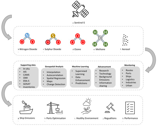
Figure 6.
Conceptual diagram elaborating the variables measured using TROPOMI, the measurement methods, and their implications.
3.4. Shipping Contribution
The section briefly discusses the contribution of shipping to air pollution according to sources found during the review. In order to obtain a wider picture, the section compiles numbers and percentages reported by different studies.
The maritime transportation sector is one of the largest and most potent sources of . Air pollution monitoring using Sentinel-5P data has demonstrated significant potential in addressing environmental challenges associated with shipping, ports, and maritime operations. Apart from shipping, iron, steel, coke, and power plants are major contributors for clusters [54]. Based on an analysis of datasets from inventories, it was concluded that, in Europe, shipping’s contributions to total emissions was 16% for , 11% for , and 5% for [101]. With a mean value of 27%, the surface concentrations of in certain ports attributed to maritime sector activities ranged from 5% to 70% of the total surface concentrations [48].
The TROPOMI data was resampled to yield vertical column density (VCD) to calculate emissions across the Yangtze River Delta (YRD) in China. The analysis revealed that emissions in Ningbo exceeded expectations, largely influenced by significant ship-related emissions [70]. Shanghai, a port city, also exhibited high levels. In comparison to Chinese emission inventory data, TROPOMI underestimated VCD in contaminated areas.
emission hotspots are observed consistently in the central areas of major cities [72]. Spatial areas of some of the cities include far more noticeable emission hotspots than their centres, which are typically seaports and industrial regions. Pseftogkas et al. [60] extracted the contribution of vessels to total emissions in the Mediterranean using Sentinel-5P data, as shown in Figure 7. columns by day of the week showed that weekend (Saturday and Sunday) concentrations were 16% to 24% lower than other days [63].
Figure 7.
Vessels’ contributions to total emissions in Mediterranean Sea.
3.5. Effect of COVID-19
In this section, studies that reported on COVID-19 are discussed with reference to emissions trends and quantification. In 2020, the COVID-19 pandemic spread around the world. It should be kept in mind that this was a unique time to explore the impact of air pollution from the maritime sector as maritime activity was ongoing to some extent during the COVID-19 pandemic, while several other activities were drastically reduced. Therefore, several studies are found in the literature that focus on a comparison of air pollution before and after the outbreak. During the COVID-19 shutdown, concentrations were lower in the majority of coastal ports and maritime transport routes, with reductions of more than 50% (for a maximum of 200 days) according to a Sentinel-5P data long-term analysis of 11 ports around the world [56].
Prior to the COVID-19 pandemic, unrestricted travel caused consistently high levels in the areas examined by [50]. There was a discernible drop in gas pollution as a result of the pandemic-induced temporary suspension of maritime industry operations to prevent COVID-19 from spreading [50]. A notable occurrence called the “lockout effect” was observed between 18 March and 13 April 2020, during which Malaysia experienced a significant drop in average concentrations across most regions [50]. This decrease was linked to the strict lockdown measures implemented due to the COVID-19 pandemic. After the lockdown, significant reductions in levels were recorded, highlighting the clear relationship between atmospheric concentrations and daily-life activities [50].
The ports of Los Angeles and Long Beach are the busiest ports in the United States [76]. Over these two ports, using TROPOMI data, levels decreased significantly during the shutdown from July 2019 to May 2020 and were expected to revert to pre-COVID-19 levels by July 2022 [53]. Hence, levels in the Los Angeles Basin decreased during the shutdown and took longer to return to normal levels according to air quality station and Sentinel-5P data. An inverse correlation between and levels was found both before and during the COVID-19 shutdown. The industrial sites in the ports region were identified as being responsible for the volatile organic hydrocarbons (VOHs), as the inverse connection between and remained during the shutdown, when non-industrial VOH sources would have declined. After COVID-19, there was an adverse impact on from increased ship and port activity in the ports of Los Angeles and Orange counties [76].
Mejía C. et al. [69] also examined air pollutants using Sentinel-5P in the Guayaquil port area in Ecuador before, during, and after the COVID-19 lockdown. The restrictions due to the pandemic lowered the transportation activity, resulting in less energy consumption, lower oil demand, and limited internal travel. These alterations in transportation patterns significantly affected air quality, causing a reduction in emissions in several regions [69].
The halt in human activity had a significant influence on Europe’s air pollution as well. The amount of emissions in March 2020 decreased significantly in large cities including Paris, London, Madrid, and Milan [73]. The decrease ranged from 14 to 31%. This decrease continued in April in Rome, Brussels, Frankfurt, Warsaw, Belgrade, Kyiv, and Moscow (34% to 51%). However, compared to the baseline, emissions in March 2020 were similar or at slightly higher levels in various areas of the UK, Poland, and Moscow, perhaps as a result of the restriction timeframe. The findings confirm that surface ozone rose during the lockdown. The observations highlight the higher surface ozone concentrations, up to 32% in regions like Germany, Italy, France, the UK, Switzerland, and Belgium, indicating a rise in surface ozone levels where emissions significantly dropped. The rise in ozone levels was confirmed by other studies as well [73]. From an analysis of 54 cities, emission reductions were observed during the first wave of COVID-19 across most cities, followed by divergent trends in subsequent periods. [72]. During the early stages of the COVID-19 pandemic in 2020, emissions from ships declined by approximately 10–20% [58].
The GAM has also been applied to , , and surface ozone across rural, urban, and suburban environments. The experience shows that the GAM is certainly a valuable instrument, especially for secondary contaminants at rural background sites. For urban and suburban stations, the most significant shutdown effect on was calculated in Spain, with a 60% reduction as a country average, followed by Italy (51%), France (51%), Portugal (47%), and Great Britain (43%). Poland (22%) and Hungary (23%), the eastern countries, showed the lowest reductions. The findings indicated that all countries had a modest improvement from April to July. Even in July, levels remained 20% below projected values in many countries, indicating a sustained impact of reduced emissions well beyond the initial lifting of lockdown restrictions. The stringent restrictions on human activities during the first wave of the COVID-19 pandemic in Europe in spring 2020 led to substantial changes in road traffic patterns. This resulted in significant reductions in and other pollutants. Monthly concentrations in terrestrial regions of the Canary Islands (Spain) decreased by approximately 40% during the lockdown. In the same time frame, the reduction was comparatively less pronounced in the maritime zones [9]. In port areas, the average concentration was molecules , reaching a peak of molecules . The measured values were an order of magnitude greater than the oceanic, non-anthropogenic background levels of molecules and were comparable to those recorded over land.
Silva et al. [79] studied the effects of the COVID-19 limits on Portugal’s air quality and presented workable mitigation options to lower air pollution. In addition to Portugal’s Air Quality data from the Portuguese Environment Agency, Sentinel-5P data for CO, , and the Absorbing Aerosol Index (AAI) from the TROPOMI sensor were used. The study reported improvement in Portugal’s air quality during the COVID-19 lockdown. and PM concentrations were significantly reduced during the lockdown period. The reductions in concentrations were more pronounced during the initial lockdown compared to subsequent periods; this was due to stricter measures during the first lockdown, including mandatory curfews, inter-municipal mobility restrictions, and permission to leave home only for essential purposes. COVID-19 restrictions led to a more significant reduction in concentrations in the Lisboa and Algarve regions compared to the Norte region. This discrepancy is likely due to the predominantly industrial nature of the Norte region, where industrial activities continued throughout the pandemic.
In the UK, tropospheric column data from TROPOMI was used to assess changes in levels at national, regional, and city scales due to the lockdown. Regionally, reductions ranged from 22 to 23% in the western areas to 29% in the south-east, with declines exceeding 40% in London [78]. In 2020, as compared to 2019, only half of the UK’s national mean rise in surface ozone and decrease in in 2020 can be attributed to changes in emissions. The remaining portion comes from variations in the weather throughout the two years, highlighting the necessity of taking weather and pollution sources into consideration when developing new abatement plans and enforcing regulations.
In Germany, by using TROPOMI and CAMS data it was detected that during the COVID-19 lockdown levels significantly decreased, by around , while increased by over ten major cities [85].
Air quality temporarily improved with lockdown measures, which reduced the emissions, in China as well [77]. Between 24 January and 6 February during the lockdown, the average daily concentrations of PM2.5, PM10, , and decreased by 19.2%, 44.7%, 21.5%, and 33.6%, respectively, compared to the same period in 2019. These were still about four times higher than the WHO guidelines (10 µg/m3 and 20 µg/m3, respectively) [77]. Using Sentinel-5P and MetOp-B satellite data, changes in were tracked during the lockdown in Shanghai and the surrounding region in China [74]. Backscattered radiances were measured by two spectrometers (TROPOMI and GOME-2). The Meteorological Operational (MetOp) satellites are equipped with the GOME-2 instruments. GOME-2B has a preset 1920 km swath and a spatial resolution of 80 km × 40 km. Liu et al. [74] measured a 42% decrease in shipping emissions for Shanghai port as a result of the lockdown. Potts et al. [78] and Xue et al. [70] estimated that emissions decreased by about 20% and 35% in China, respectively, during the lockdown (23 March to 31 May 2020).
Contrary to the studies mentioned above, rather stable air pollution levels were found over the Malta Channel region [3]. In spite of the smart lockdown protocols, given the continued existence of international seaborne trade between countries, shipping volumes during the COVID-19 pandemic essentially stayed the same [3].
Figure 8 shows the number of studies found during the review that reported changes in due to travel restrictions as a result of the COVID-19 pandemic.
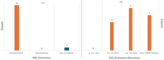
Figure 8.
Histograms of (A) effect of COVID-19 on emissions, as reported by studies; (B) the percentage decrease in emissions.
3.6. Limitations and Future Directions
Monitoring marine concentrations is currently limited by the accuracy of current satellites in terms of both spatial and temporal resolution [56]. Higher-resolution satellite sensors are required for continuous and precise estimation of marine emissions from specific ship (small-scale) sources in future. Also it is difficult to fully consider the contributions of various anthropogenic emission factors in ports. For instance, port industrial operations contribute to port levels, and ship emission reductions brought about by emission control measures do not always translate into lower tropospheric columns. Future studies on port air quality may focus on combining satellite data with in-depth emission inventories and chemical transport models. With the support of various datasets and the segregation of ship plumes, air pollution from ships can be quantified.
Table 6 shows the spatial resolution of the satellite-based sensors for monitoring pollution. Sentinel-5P’s current spatial resolution is still insufficient to distinguish between localized sources, especially when there are contributions from multiple sources such as industries near harbours [20,49]. The TEMPO instrument has the highest spatial resolution for measuring ; however, its data is limited to North America only. Sentinel-5P TROPOMI has the highest resolution for with global coverage.
Table 6.
Spatial resolution of satellite-based sensors.
As mentioned in the study by Abdullah et al. [50], the primary focus on air pollution gives a particular viewpoint on pollution in ports, which is one of the limitations of the study. Despite being useful for emissions, the research using Sentinel-5P data alone does not fully address other contaminants that contribute to air pollution in the maritime sector. There was no other research that examined the TROPOMI instrument’s global/regional sensitivity to emissions generated by specific sea-going ships in relation to their length and speed [49].
According to Georgoulias et al. [20], the ideal air conditions for detecting ship plumes are still an open subject. More research should be performed on how wind speed and viewing geometry impact surface reflectance under sun-glint, as well as plume dispersion and humidity. The ability to detect plumes from individual ships across different regions (such as ports, shorelines, and open seas) should also be investigated further. Undoubtedly, satellite remote sensing’s ability to detect ship plumes only in favourable conditions is a constraint [20]. For sun-glint conditions alone (which appear more in summer), the detectability likelihood rises to about 10% to 15%, regardless of wind speed. The likelihood is significantly greater for low-wind-speed situations alone (for all viewing geometries), surpassing 50% in certain coastal regions. Georgoulias et al. [20] used a ship emission proxy based on ship length and speed. However, the emission proxy calculation does not account for the various variables that affect ship emissions, such as weight, engine type, fuel type, and hull shape.
There is no scientific proof that ship-generated plumes can still be distinguished beneath the dense layer of land-based emission outflow [59]. Because of a ship’s non-rigid construction, dispersion, and chemical modification, there are always some areas of the plume that are at or beyond the visible detection limit of the retrieval technique (human labelling) and the TROPOMI equipment. This may result in incorrect labelling because of the structure of the waves; wind speed affects the sea surface’s reflection, which in turn affects the sensitivity of the sensors. The approach described by Pseftogkas et al. [48] is a significant step towards automated and worldwide ship emission monitoring with remote sensing, although this topic still needs more research in the satellite retrieval community. Advanced research on the exchange of pollutants between the atmosphere and the sea in marginal seas, including dry deposition fluxes, may be undertaken in the future [68].
In future, the potential for Sentinel-5P and subsequent satellite missions to track emissions from specific ships should be very beneficial for emission modelling and ship engine performance verification. With the release of version 2.2.0 of the retrieval algorithm in July 2021, notable advancements are anticipated from the TROPOMI side, but, as the comparison in Douros et al. [66] indicates, these are probably not going to be sufficient to close the gap with the winter-period modelled columns. Model sensitivity experiments with different chemistry and vertical mixing schemes, as well as other enhancements to the input data, including emissions and their injection heights, may also be necessary to determine the causes of these differences in columns.
Strict international regulations are designed to mitigate emissions from maritime shipping. But, the lack of a comprehensive global monitoring system poses challenges in verifying compliance [71]. Sentinel-5P data can be used more effectively for monitoring compliance with the regulations. Skipper et al. [76] analysed the impact of Los Angeles ports to check if there was increased activity after the COVID-19 pandemic or not. Further research into the impact of supply chain disruptions on air quality at ports worldwide would help determine whether similar effects were observed in other port regions or if they were confined to specific locations.
TROPOMI underestimated total column levels, with a mean percentage difference of −12%, and failed to capture pollution spikes resulting from rush hour traffic emissions or the accumulation of pollutants during sea-breeze events [55]. A sensitivity analysis indicated that the overall uncertainty estimation in urban areas was 40–63% [70]. Measurement frequency, cloud cover, and large spatial resolution prevent the assessment of air pollution in cities [69]. As a result, downscaling, using interpolation methods, is critical for continuous air quality monitoring at a finer scale. The enhanced horizontal resolution in the regional CAMS ensemble mean and the LOTOS-EUROS model enhances surface-level pollution estimations. However, these models consistently overpredict concentrations at elevated altitudes, suggesting excessive vertical mixing and surplus representation over the North Sea [64]. at the locations of power stations (Martin Lake, Limestone, and Sam Seyour) was significantly underestimated by TROPOMI [84,110]. A region with atmospheric conditions that result in a short lifetime could be the reason for this. Another explanation might be that the model’s / ratio was underestimated because of the large grid-cell size. TROPOMI does not fully account for the amount of emissions from power plants and their surroundings, even after applying all known modifications over big power plant plumes.
Figure 9 illustrates the connection between the sensor, its limitations, and the intermediate distribution of subjects across various stages, providing insights into the impacts of these limitations. The width of each link is proportional, providing a visual representation of dependencies. The diagram highlights the subjects that can be improved by improving the sensor’s capabilities.
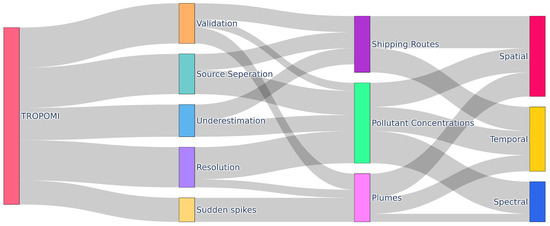
Figure 9.
Sankey diagram explaining the limitations and the relationships between different factors.
The satellite data was generally less accurate than in situ data because of the limitations of current satellite-based sensors [35,98]. Satellite-based GHG monitoring faces challenges in capturing urban-scale variations when comparing satellite observations (TROPOMI, OCO-2, OCO-3, GOSAT, GOSAT-2) with ground-based measurements (EM27/SUN) in Seoul [111]. While strong correlations were observed, biases due to aerosols and sunlight variability highlight the need for integrated validation approaches in high-emission urban areas.
The combination of remote sensing data with bottom up inventories and atmospheric modelling improved surveillance even more [87]. However, the comparison of top-down and bottom-up measurements was still an important limitation, especially for marine areas, where measurements are still a problem. Challenges persist in precise calculation of emissions exclusively caused by maritime operations [112]. The Copernicus Marine Service platform releases real-time emission heatmaps [113]. These can be integrated with Port State Control inspection databases to enable risk-based inspections for ships entering the European Citizen Action Service (ECAS). Filling these gaps with the help of increasing the number of satellite images and enhancing the sensors is critical if the goals of the Paris Agreement are to be met, and if emission reduction is to become the most effective strategy for climate change mitigation. The current review is limited by only exploring two databases; articles from other databases and non-scholarly sources could be included to further broaden the scope of the study.
4. Conclusions
This review provides a comprehensive understanding of the current advancements for monitoring maritime air pollution using Sentinel satellite data. For the systematic review, first, a Web of Science and Scopus database search was performed using specific keywords. VOSviewer was then used for the identification of collective themes in the articles. Lastly, the final article selection was performed through detailed scrutinization following the PRISMA framework. A total of 70 studies were examined in detail to develop a synthesis of the relevant research to identify future directions. The main applications for Sentinel-5P data in the maritime environment are related to air pollution. Sentinel-2 data is used for water pollution and contamination while Sentinel-1 data is most useful for oil spill-related studies.
Sentinel-5P data provides state-of-the-art publicly available global satellite data for monitoring tropospheric concentrations. and plumes and emissions from vessels can be identified using TROPOMI products. In ports, cargo equipment and logistics infrastructure can be monitored to identify hotspots and enforce compliance with international regulations. ship monitoring along LNG shipping routes can aid in reducing greenhouse gas contributions and aligning with global decarbonization goals. Additionally, wind and atmospheric data can enhance ship route optimization, improving fuel efficiency and reducing carbon footprints. GIS integration offers a dynamic platform for tracking real-time emissions, assessing health risks, and optimizing operational strategies in port areas. COVID-19 restrictions brought reductions in emissions worldwide for industrial operations as well for the maritime sector. As international organizations tighten air quality regulations for maritime activities, leveraging satellite technologies will play an increasingly critical role in ensuring compliance and promoting sustainable maritime practices.
Sentinel-5P was found to underestimate pollution concentrations; therefore, it should be supported with in situ data to ensure the accuracy of the analysis. Also, the current spatial resolution is not enough to track emissions from small ships. A limitation was found in tracking transient large increases in levels as well using TROPOMI data. A higher spatial and temporal resolution is desirable for more precise estimations. Supervised classification techniques for plume detection are effective, yet they are limited because of the limitation of human vision, as some plumes are not clearly distinguishable in the images. In the presence of other contributors, it is difficult to distinguish the plumes caused by ship emissions. Wind speed and surface conditions also impact the quality of Sentinel data.
For future perspectives, challenges in source attribution, small-vessel detection, and cross-validation with Sentinel-5P data can be worked on to further improve monitoring using Sentinel-5P data. Resolution enhancement techniques such as super-resolution could also be explored to improve the spatial resolution, which would address the current gap in detecting emissions from small vessels due to resolution limits. Future satellite deployments with improved spatial resolution will result in emission source attribution. The Sentinel-5P total column product can be used to explore its potential for the maritime sector as there is currently a lack of focus on this in the literature. In situ data can be used for validation to cope with the limitations of the Sentinel data for impactful research. Sentinel-5P has the potential to be an effective instrument for tracking and enforcing environmental and health laws. It can help in maintaining international regulations and sustainable maritime practices. Sentinel-5P can be integrated with GIS for real-time monitoring, optimization of ship routes, and reducing greenhouse gas emissions for meeting the Sustainable Development Goals. The Sentinel data combined with inventories can be analysed for better estimation and long-term analysis of emissions. Spatial and temporal analyses of the concentration levels of pollutants using cloud computing platforms would be useful for exploring the effect on climate conditions and extreme events.
Funding
The contents of this article were produced within the scope of the Agenda “NEXUS Pacto de Inovação—Transição Verde e Digital para Transportes, Logística e Mobilidade”, financed by the Portuguese Recovery and Resilience Plan (PRR), with no. C645112083-00000059 (investment project no. 53).
Data Availability Statement
The data will be shared upon reasonable request.
Acknowledgments
We express our sincere gratitude to the NEXUS Agenda for enabling our participation in this significant project. The authors acknowledge the team NEXUS for their discussions. The authors also acknowledge the four anonymous reviewers who led to improvements in the manuscript.
Conflicts of Interest
The authors declare no conflict of interest.
References
- Le Traon, P.Y.; Reppucci, A.; Alvarez Fanjul, E.; Aouf, L.; Behrens, A.; Belmonte, M.; Bentamy, A.; Bertino, L.; Brando, V.E.; Kreiner, M.B.; et al. From Observation to Information and Users: The Copernicus Marine Service Perspective. Front. Mar. Sci. 2019, 6, 234. [Google Scholar] [CrossRef]
- Aschbacher, J.; Milagro-Pérez, M.P. The European Earth monitoring (GMES) programme: Status and perspectives. Remote Sens. Environ. 2012, 120, 3–8. [Google Scholar] [CrossRef]
- Saliba, M.; Azzopardi, F.; Muscat, R.; Grima, M.; Smyth, A.; Jalkanen, J.P.; Johansson, L.; Deidun, A.; Gauci, A.; Galdies, C.; et al. Trends in Vessel Atmospheric Emissions in the Central Mediterranean over the Last 10 Years and during the COVID-19 Outbreak. J. Mar. Sci. Eng. 2021, 9, 762. [Google Scholar] [CrossRef]
- Copernicus Sentinel-5P, TROPOMI Level 2 Nitrogen Dioxide Total Column Products, Version 01; European Space Agency (ESA): Paris, France, 2018. [CrossRef]
- Copernicus Sentinel-5P, TROPOMI Level 2 Nitrogen Dioxide Total Column Products, Version 02; European Space Agency (ESA): Paris, France, 2021. [CrossRef]
- Grover, A.; Kumar, S.; Kumar, A. Ship Detection Using Sentinel-1 Sar Data. Isprs Ann. Photogramm. Remote Sens. Spat. Inf. Sci. 2018, 4, 317–324. [Google Scholar] [CrossRef]
- Santamaria, C.; Alvarez, M.; Greidanus, H.; Syrris, V.; Soille, P.; Argentieri, P. Mass Processing of Sentinel-1 Images for Maritime Surveillance. Remote Sens. 2017, 9, 678. [Google Scholar] [CrossRef]
- Kurchaba, S.; van Vliet, J.; Verbeek, F.J.; Veenman, C.J. Anomalous NO2 emitting ship detection with TROPOMI satellite data and machine learning. Remote Sens. Environ. 2023, 297, 113761. [Google Scholar] [CrossRef]
- Rodriguez Valido, M.; Perez Marrero, J.; Mauro González, A.; Fabiani Bendicho, P.; Efrem Mora, C. Evaluation of the Potential of Sentinel-5P TROPOMI and AIS Marine Traffic Data for the Monitoring of Anthropogenic Activity and Maritime Transport NOx-Emissions in Canary Islands Waters. Sustainability 2023, 15, 4632. [Google Scholar] [CrossRef]
- Ziemke, J.R.; Olsen, M.A.; Witte, J.C.; Douglass, A.R.; Strahan, S.E.; Wargan, K.; Liu, X.; Schoeberl, M.R.; Yang, K.; Kaplan, T.B.; et al. Assessment and applications of NASA ozone data products derived from Aura OMI/MLS satellite measurements in context of the GMI chemical transport model. J. Geophys. Res. Atmos. 2014, 119, 5671–5699. [Google Scholar] [CrossRef]
- García, O.E.; Sepúlveda, E.; Schneider, M.; Hase, F.; August, T.; Blumenstock, T.; Kühl, S.; Munro, R.; Gómez-Peláez, A.J.; Hultberg, T.; et al. Consistency and quality assessment of the Metop-A/IASI and Metop-B/IASI operational trace gas products (O3, CO, N2O, CH4, and CO2) in the subtropical North Atlantic. Atmos. Meas. Tech. 2016, 9, 2315–2333. [Google Scholar] [CrossRef]
- Kramarova, N.A.; Xu, P.; Mok, J.; Bhartia, P.K.; Jaross, G.; Moy, L.; Chen, Z.; Frith, S.; DeLand, M.; Kahn, D.; et al. Decade-Long Ozone Profile Record From Suomi NPP OMPS Limb Profiler: Assessment of Version 2.6 Data. Earth Space Sci. 2024, 11, e2024EA003707. [Google Scholar] [CrossRef]
- Piters, A.J.M.; Bramstedt, K.; Lambert, J.C.; Kirchhoff, B. Overview of SCIAMACHY validation: 2002–2004. Atmos. Chem. Phys. 2006, 6, 127–148. [Google Scholar] [CrossRef]
- Parker, R.J.; Webb, A.; Boesch, H.; Somkuti, P.; Barrio Guillo, R.; Di Noia, A.; Kalaitzi, N.; Anand, J.S.; Bergamaschi, P.; Chevallier, F.; et al. A decade of GOSAT Proxy satellite CH4 observations. Earth Syst. Sci. Data 2020, 12, 3383–3412. [Google Scholar] [CrossRef]
- Acker, S.J.; Holloway, T.; Harkey, M.K. Satellite Detection of NO2 Distributions and Comparison with Ground-Based Concentrations. EGUsphere 2025, 2025, 1–39. [Google Scholar] [CrossRef]
- Choi, H.; Liu, X.; Jeong, U.; Chong, H.; Kim, J.; Ahn, M.H.; Ko, D.H.; Lee, D.W.; Moon, K.J.; Lee, K.M. Geostationary Environment Monitoring Spectrometer (GEMS) polarization characteristics and correction algorithm. Atmos. Meas. Tech. 2024, 17, 145–164. [Google Scholar] [CrossRef]
- Lee, H.J.; Kim, N.R.; Shin, M.Y. Capabilities of satellite Geostationary Environment Monitoring Spectrometer (GEMS) NO2 data for hourly ambient NO2 exposure modeling. Environ. Res. 2024, 261, 119633. [Google Scholar] [CrossRef]
- Secretariat, U. United Nations Conference on Trade and Development (UNCTAD) Review of Maritime Transport 2002. Available online: https://unctad.org/publication/review-maritime-transport-2023 (accessed on 27 September 2023).
- Hasan, M. Analyzing the Blue Economy Potential of Pakistan’s Maritime Sector. Qlantic J. Soc. Sci. Humanit. 2024, 5, 202–209. [Google Scholar] [CrossRef]
- Georgoulias, A.K.; Boersma, K.F.; van Vliet, J.; Zhang, X.; van der A, R.; Zanis, P.; de Laat, J. Detection of NO2 pollution plumes from individual ships with the TROPOMI/S5P satellite sensor. Environ. Res. Lett. 2020, 15, 124037. [Google Scholar] [CrossRef]
- Bodansky, D. Chapter.17 Regulating Greenhouse Gas Emissions from Ships: The Role of the International Maritime Organization; Brill|Nijhoff: Leiden, The Netherlands, 2018; pp. 478–501. [Google Scholar] [CrossRef]
- Monteiro, A.; Russo, M.; Gama, C.; Borrego, C. Impact of SO2 shipping emissions on air quality: The airship project. WIT Trans. Ecol. Environ. 2018, 230, 429–437. [Google Scholar]
- Viana, M.; Hammingh, P.; Colette, A.; Querol, X.; Degraeuwe, B.; de Vlieger, I.; van Aardenne, J. Impact of maritime transport emissions on coastal air quality in Europe. Atmos. Environ. 2014, 90, 96–105. [Google Scholar] [CrossRef]
- Wang, H.; Liu, D.; Dai, G. Review of maritime transportation air emission pollution and policy analysis. J. Ocean Univ. China 2009, 8, 283–290. [Google Scholar] [CrossRef]
- Mahía Prados, J.M.; Arias Fernández, I.; Romero Gómez, M.; Naveiro Parga, M. The decarbonisation of the maritime sector: Horizon 2050. Brodogr. Int. J. Nav. Archit. Ocean. Eng. Res. Dev. 2024, 75, 1–26. [Google Scholar]
- Sorte, S.; Rodrigues, V.; Borrego, C.; Monteiro, A. Impact of harbour activities on local air quality: A review. Environ. Pollut. 2020, 257, 113542. [Google Scholar] [CrossRef] [PubMed]
- Monteiro, A.; Sá, E.; Fernandes, A.; Gama, C.; Sorte, S.; Borrego, C.; Lopes, M. Air quality over Portugal: Now and in 2050. WIT Trans. Ecol. Environ. 2017, 210, 621–630. [Google Scholar]
- Batista, T.; Rosa, L.; Borges, F.A.; Isbaex, C.; Martins, S. Shipping Patterns at the Port of Sines: A Temporal Analysis from 2010 to 2023. Sustainability 2025, 17, 2344. [Google Scholar] [CrossRef]
- Isbaex, C.; Costa, F.d.R.F.; Batista, T. Application of GIS in the Maritime-Port Sector: A Systematic Review. Sustainability 2025, 17, 3386. [Google Scholar] [CrossRef]
- Gordin, M.D. Scientific Babel: How Science Was Done Before and After Global English; University of Chicago Press: Chicago, IL, USA, 2015. [Google Scholar]
- Morales-Alarcón, C.H.; Bodero-Poveda, E.; Villa-Yánez, H.M.; Buñay-Guisñan, P.A. Blockchain and Its Application in the Peer Review of Scientific Works: A Systematic Review. Publications 2024, 12, 40. [Google Scholar] [CrossRef]
- Wong, D. VOSviewer. Tech. Serv. Q. 2018, 35, 219–220. [Google Scholar] [CrossRef]
- Corporation for Digital Scholarship and Roy Rosenzweig Center for History and New Media. Zotero: Your Personal Research Assistant 2024. Available online: https://www.zotero.org/ (accessed on 17 June 2025).
- Page, M.J.; McKenzie, J.E.; Bossuyt, P.M.; Boutron, I.; Hoffmann, T.C.; Mulrow, C.D.; Shamseer, L.; Tetzlaff, J.M.; Akl, E.A.; Brennan, S.E.; et al. The PRISMA 2020 statement: An updated guideline for reporting systematic reviews. BMJ 2021, 372, n71. [Google Scholar] [CrossRef]
- Christiani, P.; Rana, P.; Räsänen, A.; Pitkänen, T.P.; Tolvanen, A. Detecting Spatial Patterns of Peatland Greenhouse Gas Sinks and Sources with Geospatial Environmental and Remote Sensing Data. Environ. Manag. 2024, 74, 461–478. [Google Scholar] [CrossRef]
- Sjögersten, S.; Ledger, M.; Siewert, M.; de la Barreda-Bautista, B.; Sowter, A.; Gee, D.; Foody, G.; Boyd, D.S. Optical and radar Earth observation data for upscaling methane emissions linked to permafrost degradation in sub-Arctic peatlands in northern Sweden. Biogeosciences 2023, 20, 4221–4239. [Google Scholar] [CrossRef]
- Pointner, G.; Bartsch, A.; Dvornikov, Y.A.; Kouraev, A.V. Mapping potential signs of gas emissions in ice of Lake Neyto, Yamal, Russia, using synthetic aperture radar and multispectral remote sensing data. Cryosphere 2021, 15, 1907–1929. [Google Scholar] [CrossRef]
- Lohberger, S.; Stängel, M.; Atwood, E.C.; Siegert, F. Spatial evaluation of Indonesia’s 2015 fire-affected area and estimated carbon emissions using Sentinel-1. Glob. Change Biol. 2018, 24, 644–654. [Google Scholar] [CrossRef] [PubMed]
- Tuy, S.; Lee, H.S.; Chreng, K. Integrated assessment of offshore wind power potential using Weather Research and Forecast (WRF) downscaling with Sentinel-1 satellite imagery, optimal sites, annual energy production and equivalent CO2 reduction. Renew. Sustain. Energy Rev. 2022, 163, 112501. [Google Scholar] [CrossRef]
- Xu, Z.; Zhang, H.; Wang, Y.; Wang, X.; Xue, S.; Liu, W. Dynamic detection of offshore wind turbines by spatial machine learning from spaceborne synthetic aperture radar imagery. J. King Saud Univ. Comput. Inf. Sci. 2022, 34, 1674–1686. [Google Scholar] [CrossRef]
- Wang, H.; Fan, X.; Jian, H.; Yan, F. Exploiting the Matched Filter to Improve the Detection of Methane Plumes with Sentinel-2 Data. Remote Sens. 2024, 16, 1023. [Google Scholar] [CrossRef]
- Varon, D.J.; Jervis, D.; Pandey, S.; Gallardo, S.L.; Balasus, N.; Yang, L.H.; Jacob, D.J. Quantifying NO(x) point sources with Landsat and Sentinel-2 satellite observations of NO(2) plumes. Proc. Natl. Acad. Sci. USA 2024, 121, e2317077121. [Google Scholar] [CrossRef]
- Bilgiç, E.; Tuna Tuygun, G.; Gündüz, O. Development of an emission estimation method with satellite observations for significant forest fires and comparison with global fire emission inventories: Application to catastrophic fires of summer 2021 over the Eastern Mediterranean. Atmos. Environ. 2023, 308, 119871. [Google Scholar] [CrossRef]
- Mamić, L.; Gašparović, M.; Kaplan, G. Developing PM2.5 and PM10 prediction models on a national and regional scale using open-source remote sensing data. Environ. Monit. Assess. 2023, 195, 644. [Google Scholar] [CrossRef]
- Yang, Q.; Yuan, Q.; Li, T. Ultrahigh-resolution PM2.5 estimation from top-of-atmosphere reflectance with machine learning: Theories, methods, and applications. Environ. Pollut. 2022, 306, 119347. [Google Scholar] [CrossRef]
- Tabunschik, V.; Gorbunov, R.; Bratanov, N.; Gorbunova, T.; Mirzoeva, N.; Voytsekhovskaya, V. Fatala River Basin (Republic of Guinea, Africa): Analysis of Current State, Air Pollution, and Anthropogenic Impact Using Geoinformatics Methods and Remote Sensing Data. Sustainability 2023, 15, 15798. [Google Scholar] [CrossRef]
- Ricaud, P.; Attié, J.L.; Chalinel, R.; Pasternak, F.; Léonard, J.; Pison, I.; Pattey, E.; Thompson, R.L.; Zelinger, Z.; Lelieveld, J.; et al. The Monitoring Nitrous Oxide Sources (MIN2OS) satellite project. Remote Sens. Environ. 2021, 266, 112688. [Google Scholar] [CrossRef]
- Pseftogkas, A.; Koukouli, M.E.; Manders, A.; Segers, A.; Stavrakou, T.; Tokaya, J.; Meleti, C.; Balis, D. Maritime sector contributions on NO2 surface concentrations in major ports of the Mediterranean Basin. Atmos. Pollut. Res. 2024, 15, 102228. [Google Scholar] [CrossRef]
- Kurchaba, S.; Sokolovsky, A.; van Vliet, J.; Verbeek, F.J.; Veenman, C.J. Sensitivity analysis for the detection of NO2 plumes from seagoing ships using TROPOMI data. Remote Sens. Environ. 2024, 304, 114041. [Google Scholar] [CrossRef]
- Abdullah, M.A.; Chuah, L.; Abdullah, S.B.; Bokhari, A.; Syed, A.; Elgorban, A.M.; Akhtar, M.S.; AL-Shwaiman, H.A.; Asif, S. From port to planet: Assessing NO2 pollution and climate change effects with Sentinel-5p satellite imagery in maritime zones. Environ. Res. 2024, 257, 119328. [Google Scholar] [CrossRef]
- Soleimany, A.; Grubliauskas, R.; Šerevičienė, V. Application of satellite data and GIS services for studying air pollutants in Lithuania (case study: Kaunas city). Air Qual. Atmos. Health 2021, 14, 411–429. [Google Scholar] [CrossRef]
- Adame, J.; Gutierrez-Alvarez, I.; Bolivar, J.; Yela, M. Ground-based and OMI-TROPOMI NO2 measurements at El Arenosillo observatory: Unexpected upward trends. Environ. Pollut. 2020, 264, 114771. [Google Scholar] [CrossRef]
- Leifer, I.; Melton, C.; Blake, D.R.; Meinardi, S.; Kleinman, M. Air quality trends for the ports of Los Angeles and Long Beach spanning the covid19 crisis: Part 1. Oxidant pollutants. Atmos. Environ. 2023, 312, 119949. [Google Scholar] [CrossRef]
- Wang, K.; Wu, K.; Wang, C.; Tong, Y.; Gao, J.; Zuo, P.; Zhang, X.; Yue, T. Identification of NOx hotspots from oversampled TROPOMI NO2 column based on image segmentation method. Sci. Total Environ. 2022, 803, 150007. [Google Scholar] [CrossRef]
- Tzortziou, M.; Loughner, C.P.; Goldberg, D.L.; Judd, L.; Nauth, D.; Kwong, C.F.; Lin, T.; Cede, A.; Abuhassan, N. Intimately tracking NO2 pollution over the New York City—Long Island Sound land-water continuum: An integration of shipboard, airborne, satellite observations, and models. Sci. Total Environ. 2023, 897, 165144. [Google Scholar] [CrossRef]
- Wang, X.; Zhang, C.; Gao, Y.; Ji, X.; Su, W.; Liu, C. Satellite unravels recent changes in atmospheric nitrogen oxides emissions from global ocean shipping. J. Clean. Prod. 2023, 429, 139591. [Google Scholar] [CrossRef]
- Petetin, H.; Guevara, M.; Compernolle, S.; Bowdalo, D.; Bretonnière, P.A.; Enciso, S.; Jorba, O.; Lopez, F.; Soret, A.; Pérez García-Pando, C. Potential of TROPOMI for understanding spatio-temporal variations in surface NO2 and their dependencies upon land use over the Iberian Peninsula. Atmos. Chem. Phys. 2023, 23, 3905–3935. [Google Scholar] [CrossRef]
- Riess, T.C.V.W.; Boersma, K.F.; van Vliet, J.; Peters, W.; Sneep, M.; Eskes, H.; van Geffen, J. Improved monitoring of shipping NO2 with TROPOMI: Decreasing NOx emissions in European seas during the COVID-19 pandemic. Atmos. Meas. Tech. 2022, 15, 1415–1438. [Google Scholar] [CrossRef]
- Kurchaba, S.; van Vliet, J.; Verbeek, F.J.; Meulman, J.J.; Veenman, C.J. Supervised Segmentation of NO2 Plumes from Individual Ships Using TROPOMI Satellite Data. Remote Sens. 2022, 14, 5809. [Google Scholar] [CrossRef]
- Pseftogkas, A.; Koukouli, M.E.; Skoulidou, I.; Balis, D.; Meleti, C.; Stavrakou, T.; Falco, L.; van Geffen, J.; Eskes, H.; Segers, A.; et al. A New Separation Methodology for the Maritime Sector Emissions over the Mediterranean and Black Sea Regions. Atmosphere 2021, 12, 1478. [Google Scholar] [CrossRef]
- van der A, R.J.; Ding, J.; Eskes, H. Monitoring European anthropogenic NOx emissions from space. Atmos. Chem. Phys. 2024, 24, 7523–7534. [Google Scholar] [CrossRef]
- Kim, J.; Emmerich, M.T.M.; Voors, R.; Ording, B.; Lee, J.S. A Systematic Approach to Identify Shipping Emissions Using Spatio-Temporally Resolved TROPOMI Data. Remote Sens. 2023, 15, 3453. [Google Scholar] [CrossRef]
- Goldberg, D.L.; Anenberg, S.C.; Kerr, G.H.; Mohegh, A.; Lu, Z.; Streets, D.G. TROPOMI NO2 in the United States: A Detailed Look at the Annual Averages, Weekly Cycles, Effects of Temperature, and Correlation With Surface NO2 Concentrations. Earth’s Future 2021, 9, e2020EF001665. [Google Scholar] [CrossRef]
- Riess, T.C.V.W.; Boersma, K.F.; Van Roy, W.; de Laat, J.; Dammers, E.; van Vliet, J. To new heights by flying low: Comparison of aircraft vertical NO2 profiles to model simulations and implications for TROPOMI NO2 retrievals. Atmos. Meas. Tech. 2023, 16, 5287–5304. [Google Scholar] [CrossRef]
- Thompson, A.M.; Kollonige, D.E.; Stauffer, R.M.; Kotsakis, A.E.; Abuhassan, N.; Lamsal, L.N.; Swap, R.J.; Blake, D.R.; Townsend-Small, A.; Wecht, H.D. Two Air Quality Regimes in Total Column NO2 Over the Gulf of Mexico in May 2019: Shipboard and Satellite Views. Earth Space Sci. 2023, 10, e2022EA002473. [Google Scholar] [CrossRef]
- Douros, J.; Eskes, H.; van Geffen, J.; Boersma, K.F.; Compernolle, S.; Pinardi, G.; Blechschmidt, A.M.; Peuch, V.H.; Colette, A.; Veefkind, P. Comparing Sentinel-5P TROPOMI NO2 column observations with the CAMS regional air quality ensemble. Geosci. Model Dev. 2023, 16, 509–534. [Google Scholar] [CrossRef]
- Alberti, C.; Tu, Q.; Hase, F.; Makarova, M.V.; Gribanov, K.; Foka, S.C.; Zakharov, V.; Blumenstock, T.; Buchwitz, M.; Diekmann, C.; et al. Investigation of spaceborne trace gas products over St Petersburg and Yekaterinburg, Russia, by using COllaborative Column Carbon Observing Network (COCCON) observations. Atmos. Meas. Tech. 2022, 15, 2199–2229. [Google Scholar] [CrossRef]
- Farahat, A.; El-Kork, N.; Singh, R.P.; Jing, F. Possible Overestimation of Nitrogen Dioxide Outgassing during the Beirut 2020 Explosion. Remote Sens. 2022, 14, 6377. [Google Scholar] [CrossRef]
- Mejía C., D.; Alvarez, H.; Zalakeviciute, R.; Macancela, D.; Sanchez, C.; Bonilla, S. Sentinel satellite data monitoring of air pollutants with interpolation methods in Guayaquil, Ecuador. Remote Sens. Appl. Soc. Environ. 2023, 31, 100990. [Google Scholar] [CrossRef]
- Xue, R.; Wang, S.; Zhang, S.; He, S.; Liu, J.; Tanvir, A.; Zhou, B. Estimating city NOx emissions from TROPOMI high spatial resolution observations—A case study on Yangtze River Delta, China. Urban Clim. 2022, 43, 101150. [Google Scholar] [CrossRef]
- Wang, Y.; Xu, G.; Chen, L.; Chen, K. Characteristics of Air Pollutant Distribution and Sources in the East China Sea and the Yellow Sea in Spring Based on Multiple Observation Methods. Remote Sens. 2023, 15, 3262. [Google Scholar] [CrossRef]
- Lonsdale, C.R.; Sun, K. Nitrogen oxides emissions from selected cities in North America, Europe, and East Asia observed by the TROPOspheric Monitoring Instrument (TROPOMI) before and after the COVID-19 pandemic. Atmos. Chem. Phys. 2023, 23, 8727–8748. [Google Scholar] [CrossRef]
- Souri, A.H.; Chance, K.; Bak, J.; Nowlan, C.R.; González Abad, G.; Jung, Y.; Wong, D.C.; Mao, J.; Liu, X. Unraveling pathways of elevated ozone induced by the 2020 lockdown in Europe by an observationally constrained regional model using TROPOMI. Atmos. Chem. Phys. 2021, 21, 18227–18245. [Google Scholar] [CrossRef]
- Liu, S.; Li, X.; Li, J.; Shu, L.; Fu, T.M.; Yang, X.; Zhu, L. Observing network effect of shipping emissions from space: A natural experiment in the world’s busiest port. PNAS Nexus 2023, 2, pgad391. [Google Scholar] [CrossRef]
- Solberg, S.; Walker, S.E.; Schneider, P.; Guerreiro, C. Quantifying the Impact of the Covid-19 Lockdown Measures on Nitrogen Dioxide Levels throughout Europe. Atmosphere 2021, 12, 131. [Google Scholar] [CrossRef]
- Skipper, T.N.; Kaiser, J.; Odman, M.T.; Hasheminassab, S.; Russell, A.G. Local scale air quality impacts in the Los Angeles Basin from increased port activity during 2021 supply chain disruptions. Environ. Sci. Atmos. 2024, 4, 321–329. [Google Scholar] [CrossRef]
- Filonchyk, M.; Yan, H.; Hurynovich, V.; Wang, Z. Impact of COVID-19 pandemic on air quality changes in Shanghai, China. Environ. Forensics 2022, 23, 1–6. [Google Scholar] [CrossRef]
- Potts, D.A.; Marais, E.A.; Boesch, H.; Pope, R.J.; Lee, J.; Drysdale, W.; Chipperfield, M.P.; Kerridge, B.; Siddans, R.; Moore, D.P.; et al. Diagnosing air quality changes in the UK during the COVID-19 lockdown using TROPOMI and GEOS-Chem. Environ. Res. Lett. 2021, 16, 054031. [Google Scholar] [CrossRef]
- Silva, A.C.T.; Branco, P.T.B.S.; Ferrini Rodrigues, P.; Sousa, S.I.V. Sustainable policies for air pollution reduction after COVID-19 pandemic: Lessons learnt from the impact of the different lockdown periods on air quality. Sustain. Dev. 2023, 31, 959–975. [Google Scholar] [CrossRef]
- Nurhisanah, S.; Hasyim, H. Environmental health risk assessment of sulfur dioxide (SO2) at workers around in combined cycle power plant (CCPP). Heliyon 2022, 8, e09388. [Google Scholar] [CrossRef]
- Schmidt, S.; Kinne, J.; Lautenbach, S.; Blaschke, T.; Lenz, D.; Resch, B. Greenwashing in the US metal industry? A novel approach combining SO2 concentrations from satellite data, a plant-level firm database and web text mining. Sci. Total Environ. 2022, 835, 155512. [Google Scholar] [CrossRef]
- Sullivan, J.T.; Berkoff, T.; Gronoff, G.; Knepp, T.; Pippin, M.; Allen, D.; Twigg, L.; Swap, R.; Tzortziou, M.; Thompson, A.M.; et al. The Ozone Water–Land Environmental Transition Study: An Innovative Strategy for Understanding Chesapeake Bay Pollution Events. Bull. Am. Meteorol. Soc. 2019, 100, 291–306. [Google Scholar] [CrossRef]
- Wu, S.; Lee, H.J.; Anderson, A.; Liu, S.; Kuwayama, T.; Seinfeld, J.H.; Kleeman, M.J. Direct measurements of ozone response to emissions perturbations in California. Atmos. Chem. Phys. 2022, 22, 4929–4949. [Google Scholar] [CrossRef]
- Goldberg, D.L.; Harkey, M.; de Foy, B.; Judd, L.; Johnson, J.; Yarwood, G.; Holloway, T. Evaluating NOx emissions and their effect on O3 production in Texas using TROPOMI NO2 and HCHO. Atmos. Chem. Phys. 2022, 22, 10875–10900. [Google Scholar] [CrossRef]
- Balamurugan, V.; Chen, J.; Wenzel, A.; Keutsch, F.N. Spatiotemporal modeling of air pollutant concentrations in Germany using machine learning. Atmos. Chem. Phys. 2023, 23, 10267–10285. [Google Scholar] [CrossRef]
- Filonchyk, M.; Peterson, M.P. Changes in aerosol properties at the El Arenosillo site in Southern Europe as a result of the 2023 Canadian forest fires. Environ. Res. 2024, 260, 119629. [Google Scholar] [CrossRef]
- Zhang, S.; Ma, J.; Zhang, X.; Guo, C. Atmospheric remote sensing for anthropogenic methane emissions: Applications and research opportunities. Sci. Total Environ. 2023, 893, 164701. [Google Scholar] [CrossRef] [PubMed]
- Tu, Q.; Hase, F.; Schneider, M.; García, O.; Blumenstock, T.; Borsdorff, T.; Frey, M.; Khosrawi, F.; Lorente, A.; Alberti, C.; et al. Quantification of CH4 emissions from waste disposal sites near the city of Madrid using ground- and space-based observations of COCCON, IASI. Atmos. Chem. Phys. 2022, 22, 295–317. [Google Scholar] [CrossRef]
- Tu, Q.; Hase, F.; Blumenstock, T.; Kivi, R.; Heikkinen, P.; Sha, M.K.; Raffalski, U.; Landgraf, J.; Lorente, A.; Borsdorff, T.; et al. Intercomparison of atmospheric CO2 and CH4 abundances on regional scales in boreal areas using Copernicus Atmosphere Monitoring Service (CAMS) analysis, COllaborative Carbon Column Observing Network (COCCON) spectrometers, and Sentinel-5 Precursor satellite observations. Atmos. Meas. Tech. 2020, 13, 4751–4771. [Google Scholar] [CrossRef]
- Zhang, J.; Han, G.; Mao, H.; Pei, Z.; Ma, X.; Jia, W.; Gong, W. The Spatial and Temporal Distribution Patterns of XCH4 in China: New Observations from TROPOMI. Atmosphere 2022, 13, 177. [Google Scholar] [CrossRef]
- Magro, C.; Nunes, L.; Gonçalves, O.C.; Neng, N.R.; Nogueira, J.M.F.; Rego, F.C.; Vieira, P. Atmospheric Trends of CO and CH4 from Extreme Wildfires in Portugal Using Sentinel-5P TROPOMI Level-2 Data. Fire 2021, 4, 25. [Google Scholar] [CrossRef]
- Moon, J.; Shim, C.; Seo, J.; Han, J. Evaluation of Korean methane emission sources with satellite retrievals by spatial correlation analysis. Environ. Monit. Assess. 2024, 196, 296. [Google Scholar] [CrossRef]
- Schuit, B.J.; Maasakkers, J.D.; Bijl, P.; Mahapatra, G.; van den Berg, A.W.; Pandey, S.; Lorente, A.; Borsdorff, T.; Houweling, S.; Varon, D.J.; et al. Automated detection and monitoring of methane super-emitters using satellite data. Atmos. Chem. Phys. 2023, 23, 9071–9098. [Google Scholar] [CrossRef]
- Knapp, M.; Kleinschek, R.; Hase, F.; Agustí-Panareda, A.; Inness, A.; Barré, J.; Landgraf, J.; Borsdorff, T.; Kinne, S.; Butz, A. Shipborne measurements of XCO2, XCH4, and XCO above the Pacific Ocean and comparison to CAMS atmospheric analyses and S5P/TROPOMI. Earth Syst. Sci. Data 2021, 13, 199–211. [Google Scholar] [CrossRef]
- Mahmud, K.; Mitra, B.; Uddin, M.S.; Hridoy, A.E.E.; Aina, Y.A.; Abubakar, I.R.; Rahman, S.M.; Tan, M.L.; Rahman, M.M. Temporal assessment of air quality in major cities in Nigeria using satellite data. Atmos. Environ. X 2023, 20, 100227. [Google Scholar] [CrossRef]
- Palmer, P.I.; O’Doherty, S.; Allen, G.; Bower, K.; Bösch, H.; Chipperfield, M.P.; Connors, S.; Dhomse, S.; Feng, L.; Finch, D.P.; et al. A measurement-based verification framework for UK greenhouse gas emissions: An overview of the Greenhouse gAs Uk and Global Emissions (GAUGE) project. Atmos. Chem. Phys. 2018, 18, 11753–11777. [Google Scholar] [CrossRef]
- Li, S.; Kenea, S.T.; Kim, S.; Yoo, H.J.; Joo, S.; Lee, H.; Oh, S.; Jeong, M.J.; Seo, W.; Ko, M.; et al. Latitudinal distribution and sources analysis of greenhouse gases and air pollutants observed during the 2021 Yellow Sea Air Quality campaign aboard a research vessel. Atmos. Environ. 2024, 317, 120201. [Google Scholar] [CrossRef]
- Mitra, B.; Hridoy, A.E.E.; Mahmud, K.; Uddin, M.S.; Talha, A.; Das, N.; Nath, S.K.; Shafiullah, M.; Rahman, S.M.; Rahman, M.M. Exploring Spatial and Temporal Dynamics of Red Sea Air Quality through Multivariate Analysis, Trajectories, and Satellite Observations. Remote Sens. 2024, 16, 381. [Google Scholar] [CrossRef]
- Reshi, A.R.; Pichuka, S.; Tripathi, A. Applications of Sentinel-5P TROPOMI Satellite Sensor: A Review. IEEE Sens. J. 2024, 24, 20312–20321. [Google Scholar] [CrossRef]
- Veefkind, J.; Aben, I.; McMullan, K.; Förster, H.; de Vries, J.; Otter, G.; Claas, J.; Eskes, H.; de Haan, J.; Kleipool, Q.; et al. TROPOMI on the ESA Sentinel-5 Precursor: A GMES mission for global observations of the atmospheric composition for climate, air quality and ozone layer applications. Remote Sens. Environ. 2012, 120, 70–83. [Google Scholar] [CrossRef]
- Russo, M.; Leitão, J.; Gama, C.; Ferreira, J.; Monteiro, A. Shipping emissions over Europe: A state-of-the-art and comparative analysis. Atmos. Environ. 2018, 177, 187–194. [Google Scholar] [CrossRef]
- Hsu, C.H.; Henze, D.K.; Mizzi, A.P.; González Abad, G.; He, J.; Harkins, C.; Naeger, A.R.; Lyu, C.; Liu, X.; Chan Miller, C.; et al. An Observing System Simulation Experiment Analysis of How Well Geostationary Satellite Trace-Gas Observations Constrain NOx Emissions in the US. J. Geophys. Res. Atmos. 2024, 129, e2023JD039323. [Google Scholar] [CrossRef]
- Cheng, L.; Wang, Y.; Yan, H.; Tao, J.; Wang, H.; Lin, J.; Xu, J.; Chen, L. Preliminary Global NO2 Retrieval from EMI-II Onboard GF5B/DQ1 and Comparison to TROPOMI. Remote Sens. 2024, 16, 4087. [Google Scholar] [CrossRef]
- van Geffen, J.; Boersma, K.F.; Eskes, H.; Sneep, M.; ter Linden, M.; Zara, M.; Veefkind, J.P. S5P TROPOMI NO2 slant column retrieval: Method, stability, uncertainties and comparisons with OMI. Atmos. Meas. Tech. 2020, 13, 1315–1335. [Google Scholar] [CrossRef]
- Lange, K.; Richter, A.; Bösch, T.; Zilker, B.; Latsch, M.; Behrens, L.K.; Okafor, C.M.; Bösch, H.; Burrows, J.P.; Merlaud, A.; et al. Validation of GEMS tropospheric NO2 columns and their diurnal variation with ground-based DOAS measurements. Atmos. Meas. Tech. 2024, 17, 6315–6344. [Google Scholar] [CrossRef]
- Goldberg, D.L.; Lamsal, L.N.; Loughner, C.P.; Swartz, W.H.; Lu, Z.; Streets, D.G. A high-resolution and observationally constrained OMI NO2 satellite retrieval. Atmos. Chem. Phys. 2017, 17, 11403–11421. [Google Scholar] [CrossRef]
- Hu, X.M.; Hu, J.; Gao, L.; Cai, C.; Jiang, Y.; Xue, M.; Zhao, T.; Crowell, S.M.R. Multisensor and Multimodel Monitoring and Investigation of a Wintertime Air Pollution Event Ahead of a Cold Front Over Eastern China. J. Geophys. Res. Atmos. 2021, 126, e2020JD033538. [Google Scholar] [CrossRef]
- Ma, Y.; Liu, L.; Liu, X.; Chen, J. An improved downscaled sun-induced chlorophyll fluorescence (DSIF) product of GOME-2 dataset. Eur. J. Remote Sens. 2022, 55, 168–180. [Google Scholar] [CrossRef]
- Jeffery, P.S.; Walker, K.A.; Sioris, C.E.; Boone, C.D.; Degenstein, D.; Manney, G.L.; McElroy, C.T.; Millán, L.; Plummer, D.A.; Ryan, N.J.; et al. Water vapour and ozone in the upper troposphere–lower stratosphere: Global climatologies from three Canadian limb-viewing instruments. Atmos. Chem. Phys. 2022, 22, 14709–14734. [Google Scholar] [CrossRef]
- Dimitropoulou, E.; Hendrick, F.; Pinardi, G.; Friedrich, M.M.; Merlaud, A.; Tack, F.; De Longueville, H.; Fayt, C.; Hermans, C.; Laffineur, Q.; et al. Validation of TROPOMI tropospheric NO2 columns using dual-scan multi-axis differential optical absorption spectroscopy (MAX-DOAS) measurements in Uccle, Brussels. Atmos. Meas. Tech. 2020, 13, 5165–5191. [Google Scholar] [CrossRef]
- Park, H.; Jeong, S.; Sha, M.K.; Lee, J.; Frey, M.M. Comparisons of Greenhouse Gas Observation Satellite Performances Over Seoul Using a Portable Ground-Based Spectrometer. Geophys. Res. Lett. 2024, 51, e2024GL109334. [Google Scholar] [CrossRef]
- Freitas, D.; Gervásio, H. The challenge of benchmarking carbon emissions in maritime ports. Environ. Pollut. 2024, 363, 125170. [Google Scholar] [CrossRef]
- von Schuckmann, K.; Traon, P.Y.L.; Smith, N.; Pascual, A.; Djavidnia, S.; Gattuso, J.P.; Grégoire, M.; Aaboe, S.; Alari, V.; Alexander, B.E.; et al. Copernicus Marine Service Ocean State Report, Issue 5. J. Oper. Oceanogr. 2021, 14, 1–185. [Google Scholar] [CrossRef]
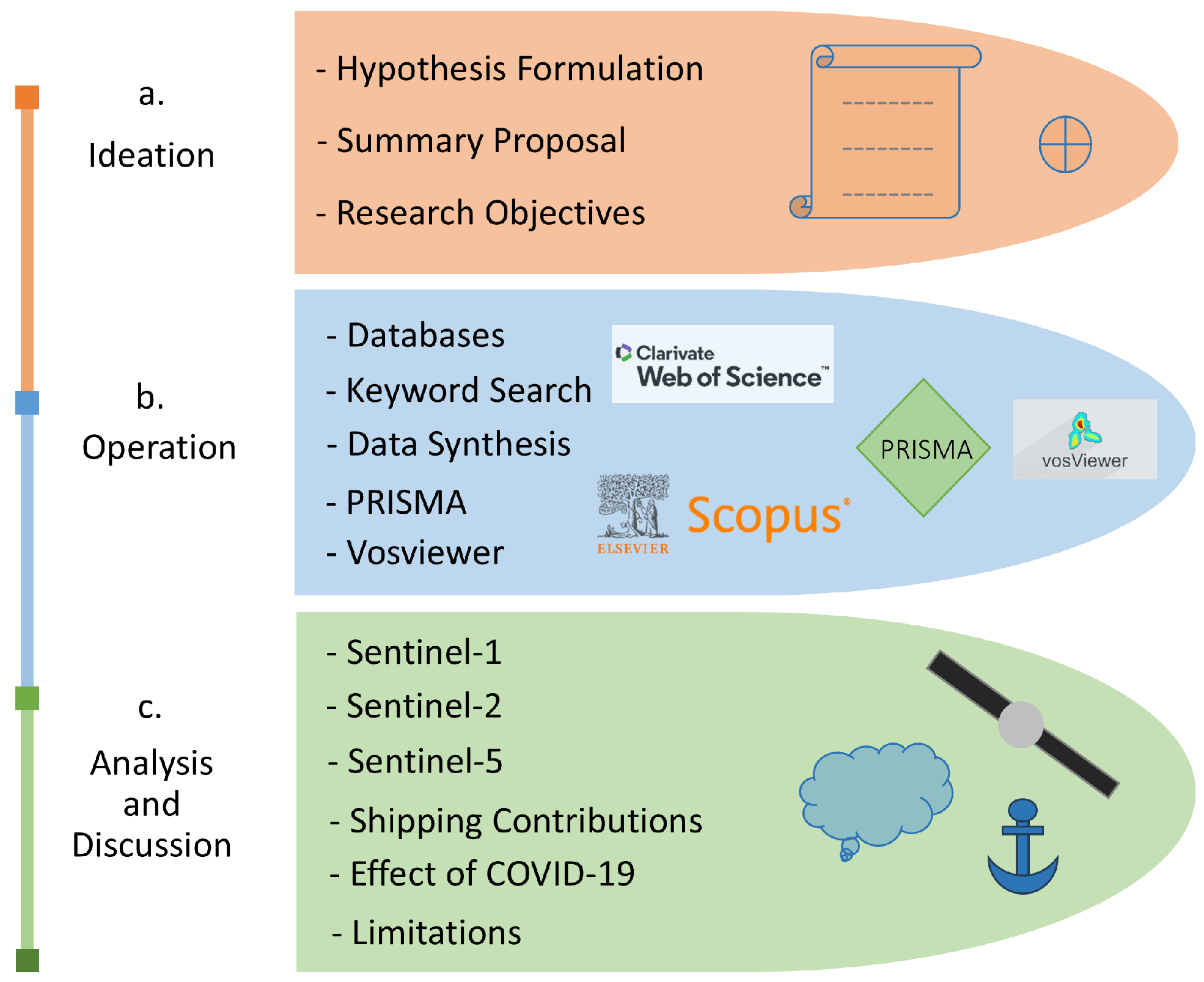
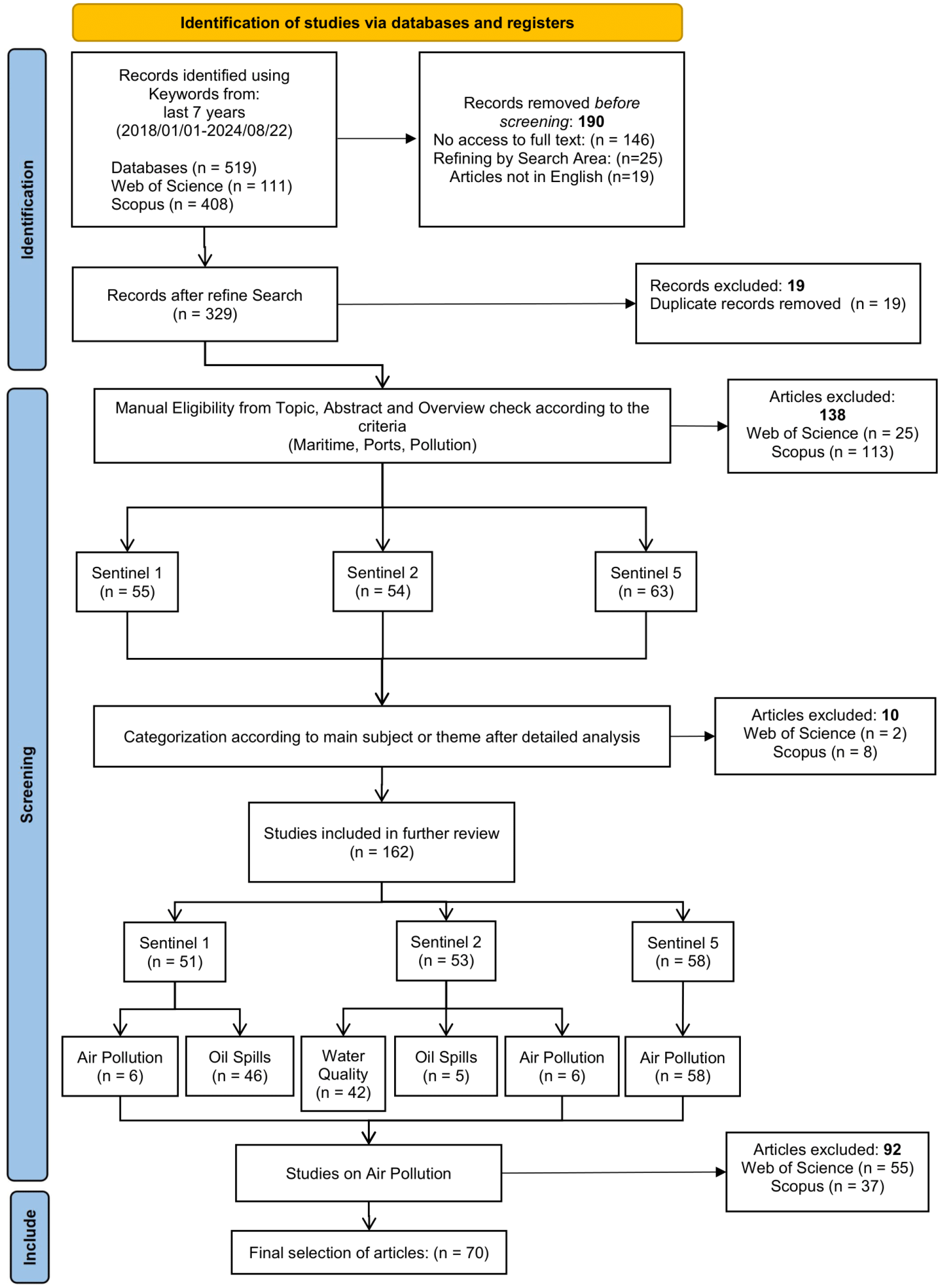
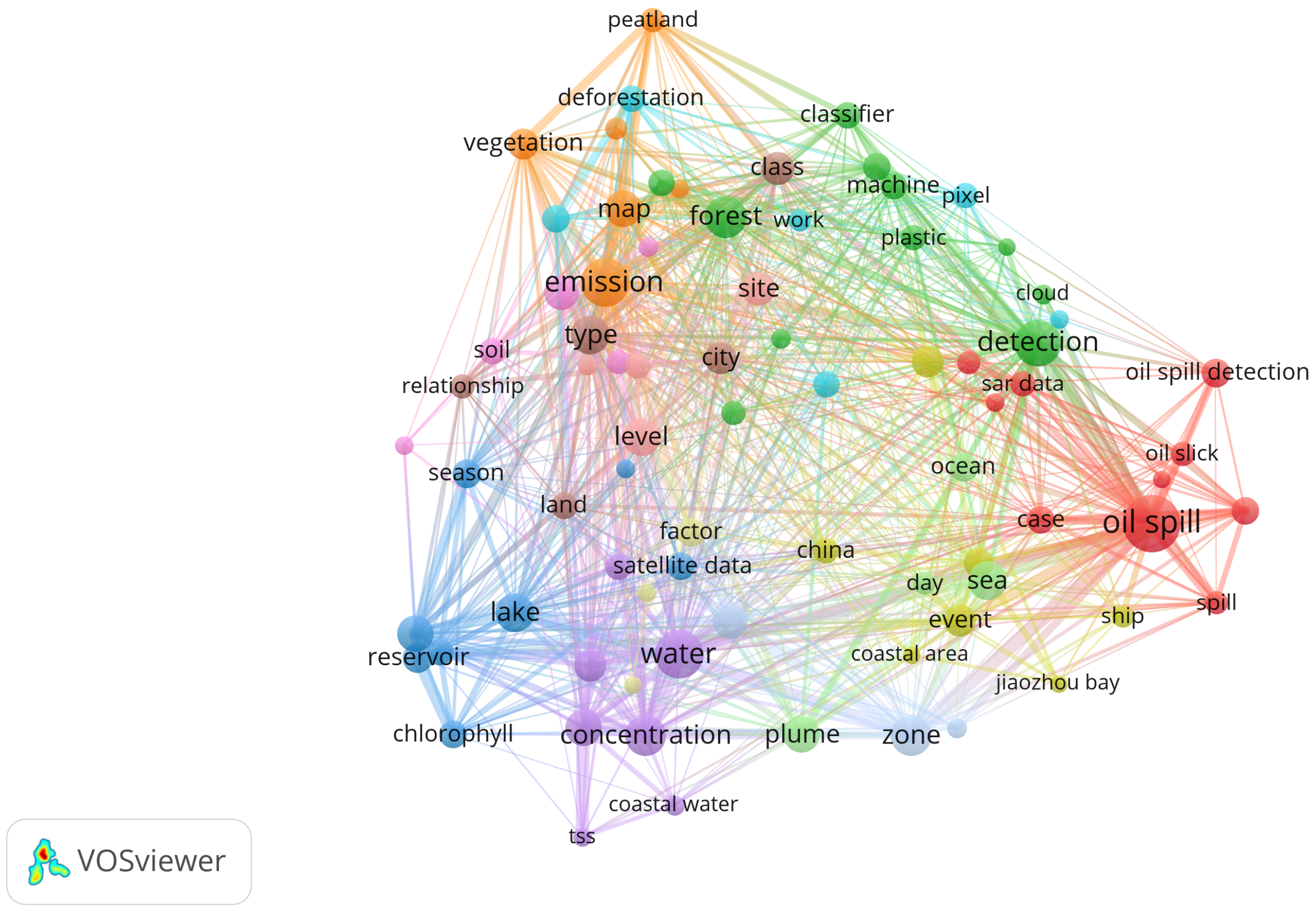
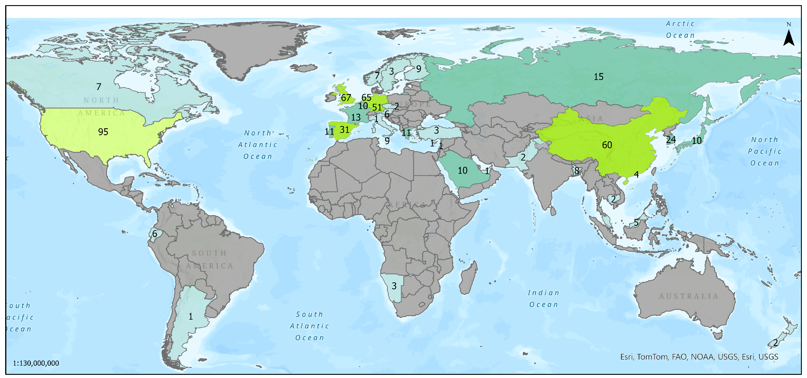
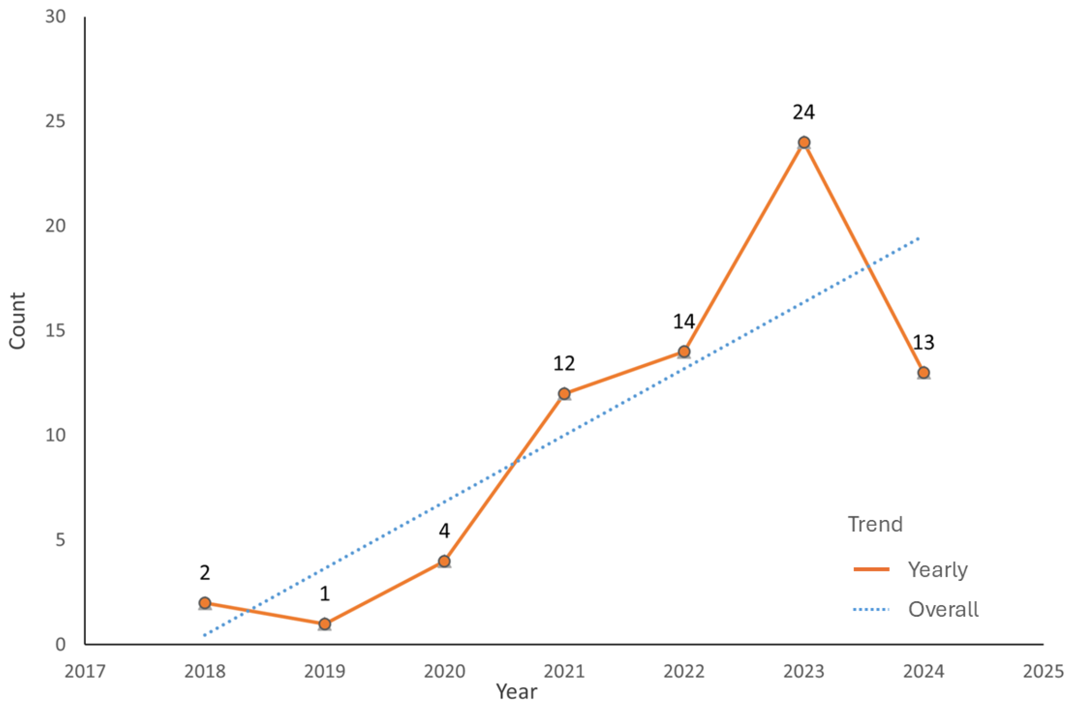
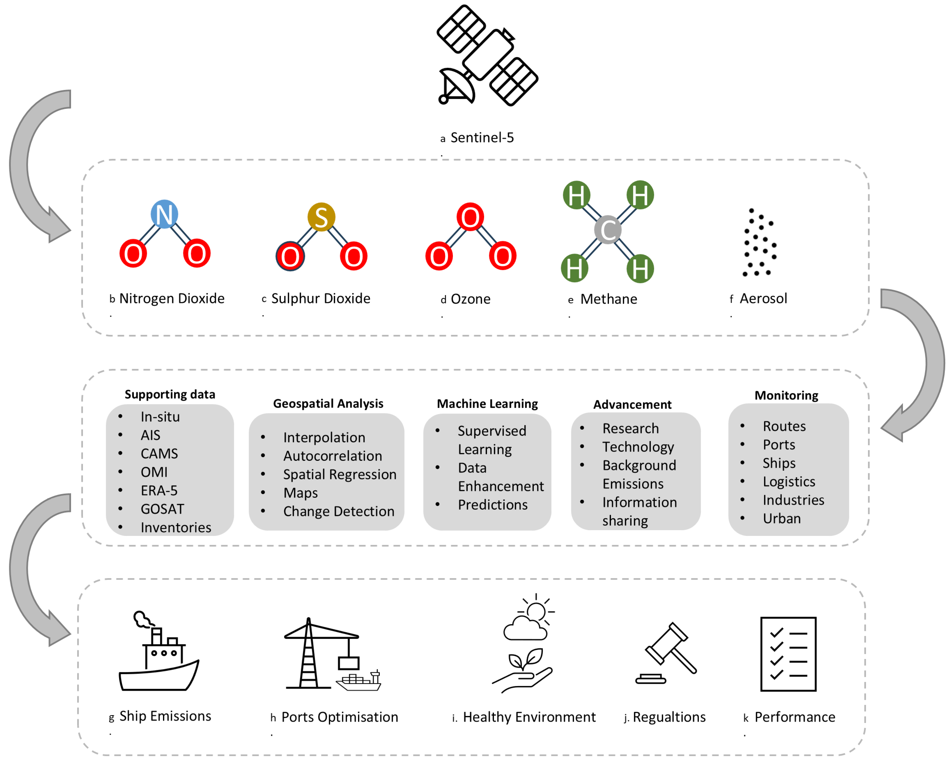
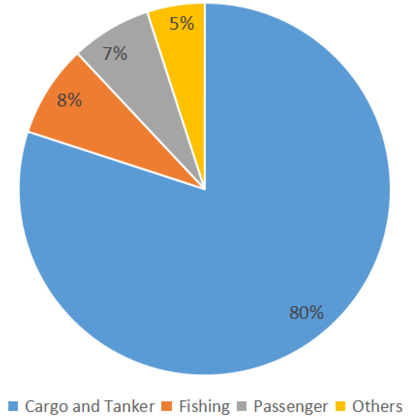

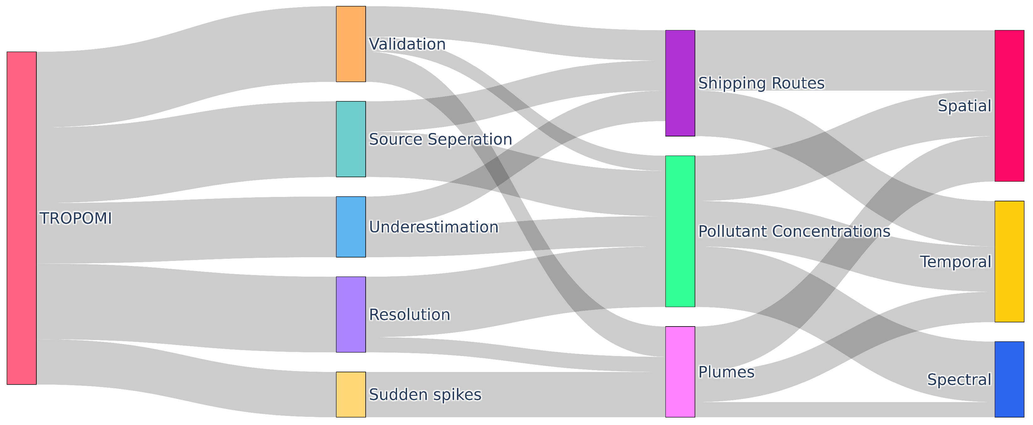
Disclaimer/Publisher’s Note: The statements, opinions and data contained in all publications are solely those of the individual author(s) and contributor(s) and not of MDPI and/or the editor(s). MDPI and/or the editor(s) disclaim responsibility for any injury to people or property resulting from any ideas, methods, instructions or products referred to in the content. |
© 2025 by the authors. Licensee MDPI, Basel, Switzerland. This article is an open access article distributed under the terms and conditions of the Creative Commons Attribution (CC BY) license (https://creativecommons.org/licenses/by/4.0/).