Article

A Full-Life-Cycle Modeling Framework for Cropland Abandonment Detection Based on Dense Time Series of Landsat-Derived Vegetation and Soil Fractions

1
College of Land Science and Technology, China Agricultural University, Beijing 100193, China
2
School of Soil and Water Conservation, Beijing Forestry University, Beijing 100038, China
3
National Geomatics Center of China, Ministry of Natural Resources, Beijing 100830, China
4
Jinan Geotechnical Investigation and Surveying Research Institute, Jinan 250013, China
*
Author to whom correspondence should be addressed.
These authors contributed equally to this work.
Remote Sens. 2025, 17(13), 2193; https://doi.org/10.3390/rs17132193
Submission received: 28 April 2025 / Revised: 20 June 2025 / Accepted: 23 June 2025 / Published: 25 June 2025

Abstract

Remotely sensed cropland abandonment monitoring is crucial for providing spatially explicit references for maintaining sustainable agricultural practices and ensuring food security. However, abandoned cropland is commonly detected based on multi-date classification or the dynamics of a single vegetation index, with the interactions between vegetation and soil time series often being neglected, leading to a failure to understand its full-life-cycle succession processes. To fill this gap, we propose a new full-life-cycle modeling framework based on the interactive trajectories of vegetation–soil-related endmembers to identify abandoned and reclaimed cropland in Jinan from 2000 to 2022. In this framework, highly accurate annual fractional vegetation- and soil-related endmember time series are generated for Jinan City for the 2000–2022 period using spectral mixture models. These are then used to integrally reconstruct temporal trajectories for complex scenarios (e.g., abandonment, weed invasion, reclamation, and fallow) using logistic and double-logistic models. The parameters of the optimization model (fitting type, change magnitude, start timing, and change duration) are subsequently integrated to develop a rule-based hierarchical identification scheme for cropland abandonment based on these complex scenarios. After applying this scheme, we observed a significant decline in green vegetation (a slope of −0.40% per year) and an increase in the soil fraction (a rate of 0.53% per year). These pathways are mostly linked to a duration between 8 and 15 years, with the beginning of the change trend around 2010. Finally, the results show that our framework can effectively separate abandoned cropland from reclamation dynamics and other classes with satisfactory precision, as indicated by an overall accuracy of 86.02%. Compared to the traditional yearly land cover-based approach (with an overall accuracy of 77.39%), this algorithm can overcome the propagation of classification errors (with product accuracy from 74.47% to 85.11%), especially in terms of improving the ability to capture changes at finer spatial scales. Furthermore, it also provides a better understanding of the whole abandonment process under the influence of multi-factor interactions in the context of specific climatic backgrounds and human disturbances, thus helping to inform adaptive abandonment management and sustainable agricultural policies.

1. Introduction

Cropland abandonment, a key type of agricultural land use change across global and local scales, refers to the practice of ceasing agricultural activity on previously farmed land and leaving it to nature [1,2]. This practice has multiple social and environment impacts, such as declines in agricultural production area and wildlife communities adapted to agroecosystems. Thus, it not only threatens food production capacity but also exacerbates challenges related to land degradation [3,4,5,6]. In the context of global urbanization and food supply/demand exacerbation, a comprehensive understanding of the detailed spatio-temporal patterns and full-life-cycle process of farmland abandonment is crucial for ensuring food security and maintaining sustainable agricultural practices.
Monitoring land abandonment is important but difficult and not routinely implemented. Aggregated statistics released by international/national organizations often fail to capture the spatial patterns of changes. Recent advancements in remote sensing technology with medium- or high-resolution data, e.g., from Landsat and Sentinel-2, have enabled detailed assessments of change processes over time [7]. However, previous maps of cropland abandonment mostly concentrate on limited time periods through data obtained using pairs of multi-date satellite images due to the difficulty of processing extensive time series data efficiently [8,9]. Fortunately, cloud-based geo-processing platforms, such as Google Earth Engine, might alleviate some of these limitations and be extendable to long-timeframe mapping [10].
The use of consistent time series in cropland modeling methods can allow for the depiction of the entire life cycle of land use and cover change processes, proving to be effective tools for detecting where, when, and how these changes occur [11]. Currently, the identification of cropland abandonment based on year-by-year classification results is widely applied [12,13]. However, this method often depends on the accuracy of land cover classification, resulting in large uncertainties regarding high-precision mapping at fine scales. In particular, abandoned cropland can easily be confused with reclaimed cropland, weed invasion, and fallow. Time series analysis (e.g., the detection of trends and breakpoints and continuous change detection and classification) incorporating indices derived from a certain number of spectral bands, such as the normalized difference vegetation index (NDVI), the leaf area index (LAI), and net primary production (NPP), has been successfully applied in understanding trends in the disturbance and recovery of cropland [14,15]. However, the spectral reflectance of agricultural land use data often differs from year to year (e.g., changes in crop type and the subsequent succession process), making it challenging to capture succession pathways before and after abandonment when using such limited information.
Given the mixed information on vegetation and soil acquired by satellites, spectral mixture analysis (SMA) can provide physically meaningful endmember abundance values at the sub-pixel scale, offering superior indicators of the interactive trajectories of cropland conversions compared to traditional vegetation indices [16,17]. Recently, a multi-temporal SMA was successfully applied for multi-seasonal Landsat and MODIS satellite imagery in order to estimate the fractional sequences of green vegetation- and soil-related endmembers [18,19]. However, to date, this interaction information pertaining to coupled elements has not yet been fully exploited to comprehensively model the full-life-cycle processes of cultivated land abandonment at the sub-pixel scale. Addressing this gap could enhance the accuracy and reliability of abandonment monitoring, contributing to the development of more effective and precise land management strategies.
In this study, we first unified a framework linking endmember dynamics with double-logistic/logistic thresholds to reconstruct full-life-cycle processes and their phase-specific metrics (soil exposure persistence and recovery trajectory) of cropland abandonment, as manifested in over 20 years of vegetation–soil fractional time series derived from Landsat series optical images. The specific objectives of this study were as follows: (1) to reconstruct the temporal trajectory of cropland abandonment using vegetation–soil endmember fractional time series; (2) to investigate the multi-dimensional thematic features of the vegetation–soil nexus; and (3) to develop a knowledge-driven identification framework for cropland abandonment scenarios. By integrating these steps, our approach realizes more efficient and high-precision monitoring of cropland abandonment and provides a comprehensive understanding of the full-life-cycle dynamics during land abandonment, therefore supporting better land management and sustainability efforts.

2. Materials and Methods
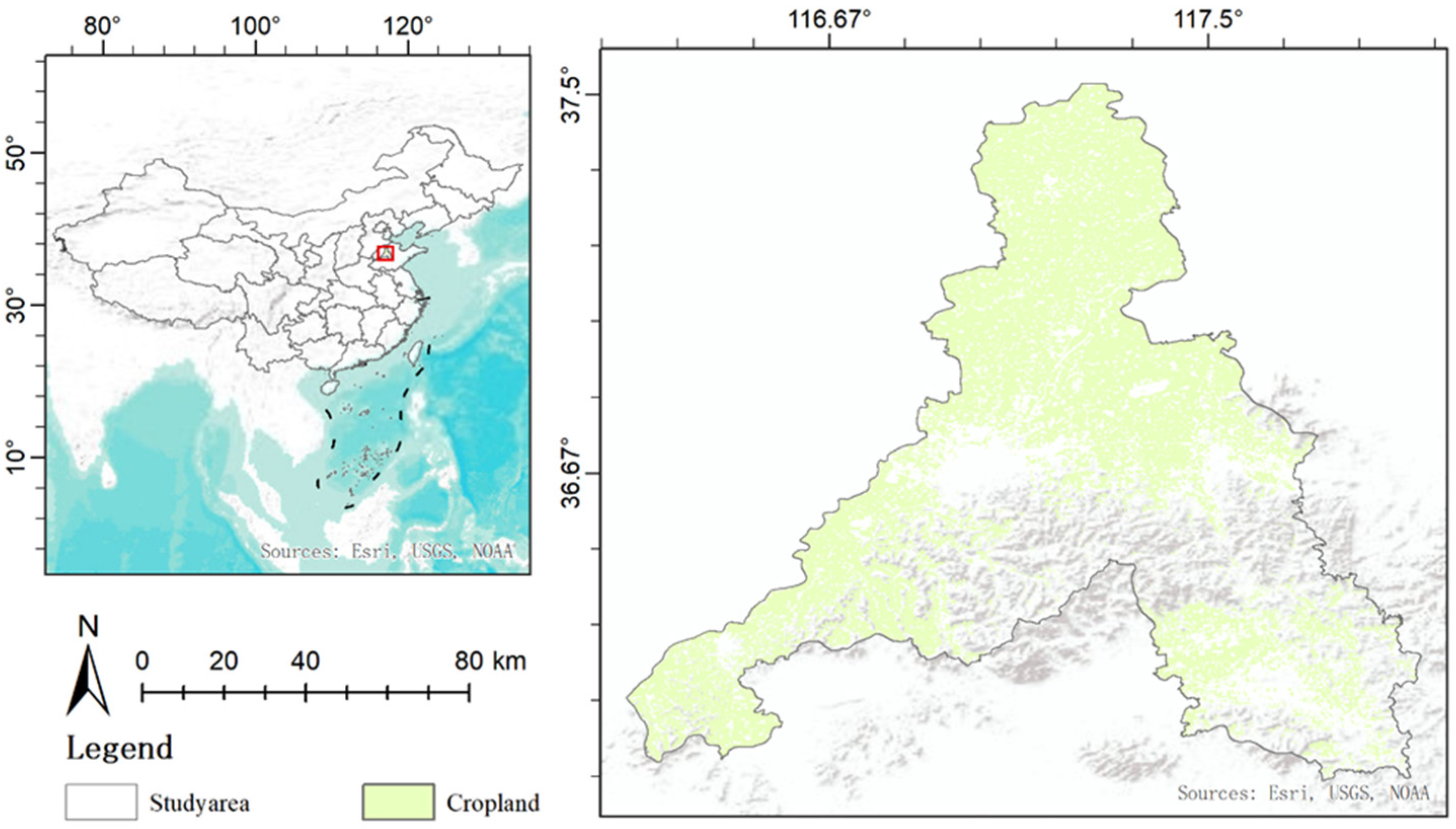
In this study, we propose a systematic technical framework for the full-life-cycle modeling of fractional endmember time series for cropland abandonment detection, motivated by the complex and dynamic nature of abandonment processes. Unlike classical abandonment monitoring based on the results of the year-by-year classification of land use cover, a full life cycle refers to the complete temporal progression of cropland abandonment, spanning three distinct but interconnected phases: first, the reduction in managed vegetation (e.g., crops or pasture), increased soil exposure, and the fragmentation of agricultural patterns; second, convergence toward stable non-agricultural land cover (e.g., bare land and degraded shrubland); and third, shrub encroachment or soil exposure under different climate conditions. These three phases often involve changes in vegetation cover and soil exposure under land use transitions over time. These changes typically exhibit distinct temporal patterns, including interactive shifts between fractional vegetation and soil endmembers (e.g., vegetation decline and soil increase, relatively stable phases, and potential vegetation recovery under climatic influences; Figure 1a). By modeling the full life cycle of these changes, it is possible to capture subtle early indicators as well as long-term stabilization phases, ensuring a more accurate and reliable detection of abandonment.
First, multi-temporal remote sensing data are utilized to construct pixel-wise fractional endmember time series using the SMA model. Then, multiple time series models, including linear, logistic, and double-logistic curve models, are applied to fit the endmember time series for each pixel. The model with the lowest root mean square error (RMSE) is selected as the optimal representation, ensuring a highly accurate depiction of temporal changes. Based on the selected optimal models, key parameters associated with cropland abandonment dynamics are extracted. Finally, these parameters are integrated with classification rules to develop a cropland abandonment detection model based on initial cropland boundary identification using multi-source data fusion (Figure 1b). By integrating multi-source data processing, time series fitting, and feature extraction techniques, the proposed framework enhances the accuracy and robustness of abandonment detection, offering a novel solution for the dynamic monitoring of land resources.

2.1. Study Area

The study area encompasses Jinan, located in Shandong Province, northern China; it represents an agro-ecological microcosm, where complex farmland transitions unfold. The region lies between approximately 36.67°N to 37.5°N latitude and 116.67°E to 117.5°E longitude, featuring a mix of agricultural land and other land cover types (Figure 2). Its climatic duality—spanning semi-arid northern plains to humid southern foothills—creates a natural laboratory for modeling divergent abandonment pathways, from drought-driven soil exposure to weed encroachment. The cropland area covers more than half of the study area. The high proportion of cropland highlights the area’s significance in agricultural activities and its potential vulnerability to land use changes. This convergence of climatic gradients, geomorphic contrasts, and socioeconomic tensions reflects the representativeness of cropland transition, positioning Jinan as a critical observatory for the development of transferable abandonment frameworks.

2.2. Data and Processes

2.2.1. Landsat Surface Reflectance Time Series (2000–2022)

We used all available Landsat 5 TM, Landsat 7 ETM+, and Landsat 8 OLI Collection 2 atmospherically corrected surface reflectance data from 2000 to 2022 for year-by-year reflectance data production using the Google Earth Engine platform. All observations with less than 50% cloud content were selected, and the cloud-covered areas were masked based on the “QA_PIXEL” band, which is a pixel quality attribute generated from the common C Function of Mask (CFMASK) algorithm [20]. The Landsat 7 ETM+ SLC-off data in 2012 and 2013 were gap-filled using the focal analysis function. Finally, all images obtained after preprocessing were fused using the NDVI maximum synthesis method to obtain annual reflectance stacks across six spectral bands (blue, green, red, near-infrared, short-wave infrared 1, and short-wave infrared 2 bands). This continuous 23-year time series enabled the pixel-level trajectory modeling of abandonment signatures with minimized sensor-induced noise.

2.2.2. Multi-Source Cropland Boundary Datasets

We determined the initial cropland boundaries using major global cropland data products, which are widely recognized for their high accuracy in global cropland and land cover monitoring (Table 1). These products, particularly those from the year 2000, were selected to extract the extent of cropland as the initial boundary for each dataset based on the definition of their respective land cover classes. To address definitional discrepancies across datasets, we ensured consistency in the classification of cropland. Subsequently, voting rules were used to integrate data from multiple sources in order to obtain the final extent of cropland. This approach can reduce uncertainty in the extraction of cropland boundaries resulting from mistakes in individual products. When the frequency of cropland occurrence in each 30 m pixel was more than 75% (frequency not less than 5), we categorized these pixels as cropland and identified the initial cropland boundary. Furthermore, we validated the cropland boundaries by comparing them with high-resolution Google Earth imagery from around 2000. Despite some limitations due to missing imagery in certain regions, the validation results were largely consistent with the boundaries identified by our model (Figure S1).

2.3. Generating Annual Continuous Vegetation–Soil Fractional Maps from Spectral Mixture Model

The spectral mixture model has the advantage of providing physically fractional surface elements through representative endmember selection, linear spectral mixture analysis, and accuracy assessments [28]. The model has been robustly demonstrated in regional and global surface element extraction, land use cover classification, and evolutionary process resolution [29,30]. Although there are variations in the spectra obtained from different sensors and at different times, the multi-temporal endmember selection scheme has been well validated regionally and globally [19,31]. Previous studies have demonstrated that three surface endmembers, namely green vegetation (GV), soil (SL), and dark material (DA), can characterize regional and global hybrid spaces [29,31]. GV represents vegetative cover that photosynthesizes on the surface; SL is the bare ground on the surface of the Earth; and DA refers to dark materials that have low reflective properties, such as bodies of water and shadows. This selection has been proven effective in agricultural contexts and land cover monitoring. This scheme presents an enhanced method for endmember selection by integrating principal component analysis (PCA) with two-dimensional scatterplot visualization.
PCA was applied to the multi-temporal dataset in order to extract principal components that encapsulate the dominant variance across both temporal and spectral dimensions, thereby enabling the identification of representative temporal snapshots for endmember selection that maximally highlight endmember variability for Landsat TM, ETM+, and OLI. Based on the ranking of the cumulative contributions of the first three principal components (Figure 3a), we carried out spectral curve selection for Landsat TM in 2000, 2008, and 2010; Landsat ETM+ in 2012 and 2013; and Landsat OLI in 2016, 2018, and 2022. By constructing two-dimensional scatterplots using a principal component emphasizing the target endmember and another orthogonal component, 200–300 spectrally pure pixels were identified at the vertices of the convex hull. These pixels were then mapped back to the original image, and their spectral curves were extracted. This approach ensures temporally representative and spectrally distinct endmember selection [29], enabling precise spectral unmixing and dynamic analyses for remote sensing applications. Finally, the mean spectral curves of the specific endmembers selected from all representative time steps were aggregated and used as the standard spectral curves (Figure 3).

2.4. Cropland Abandonment Detection

An SMA-generated fractional time series can reflect the vegetation and soil conditions of cropland, and time series fitting can allow for the identification of the path of evolution and the characterization of the different stages of abandonment through multi-phase-specific metric mining. Thus, the novel integration engine identifies phase transitions through time series analysis. Therefore, the algorithm of cropland abandonment detection from the full-life-cycle modeling of fractional endmember time series, as illustrated in Figure 1b, consists of two main stages: The first stage focuses on reconstructing the time series of key fractional endmembers to capture the temporal dynamics of land cover, followed by the parameter identification of trends, point of change, change magnitude, and change duration. The second stage involves an analysis of the parameter-based temporal variations across different endmember time series to detect significant changes in land use, particularly in areas where agricultural activities have ceased.

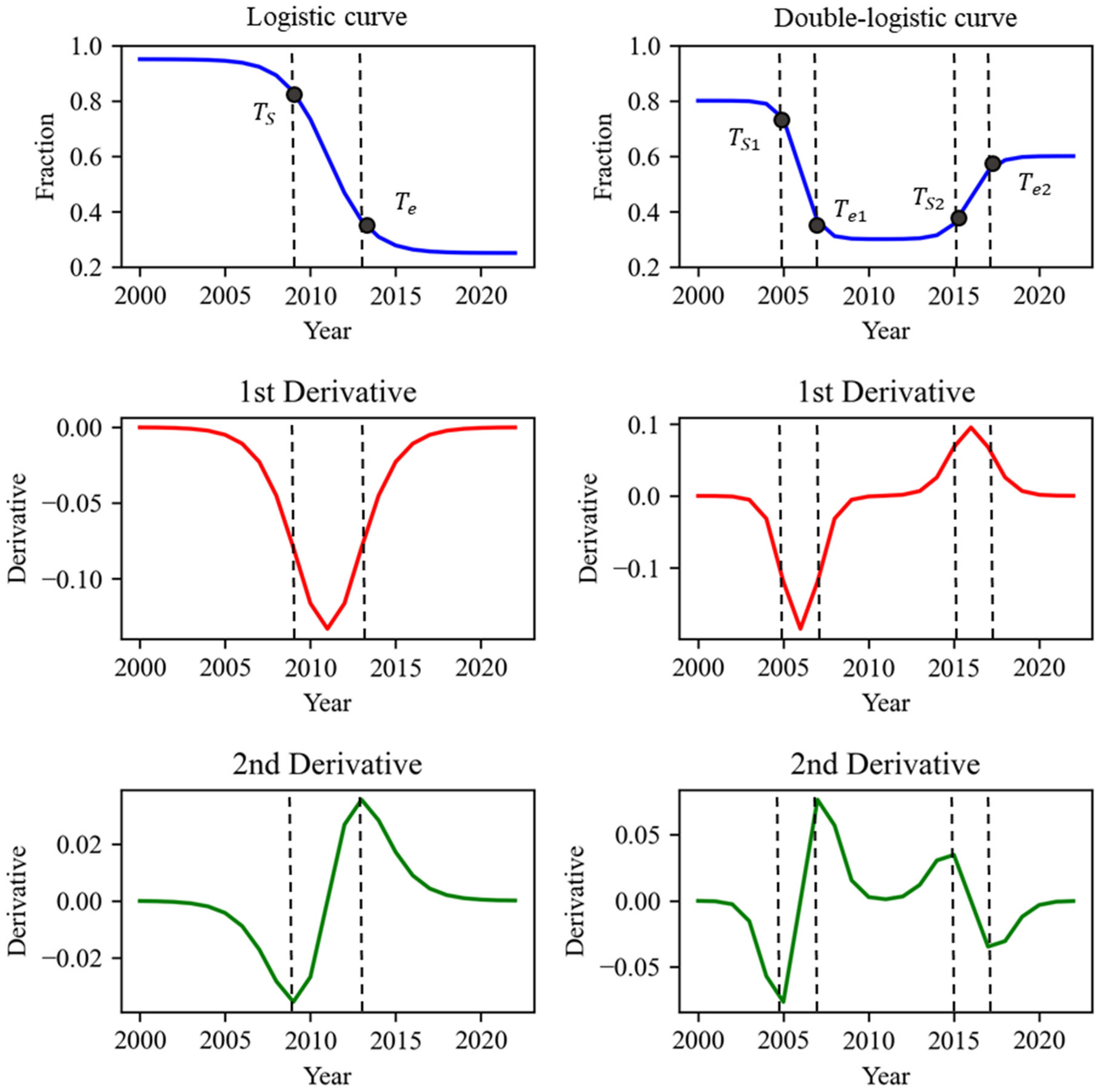
2.4.1. Modeling Temporal Trajectories in Vegetation–Soil Endmember Time Series

This modeling leverages time series imagery of surface endmembers such as vegetation and soil to model the entire process of cropland abandonment through adaptive time series fitting. By reconstructing the abandonment trajectory across different pathways, the method extracts key feature parameters essential for detecting cropland abandonment.
Considering the distinct temporal evolution patterns of vegetation and soil endmembers, the method accounts for these variations when modeling cropland abandonment. In arid regions, where natural vegetation recovery is limited, the time series of vegetation and soil endmembers typically follow a logistic curve, reflecting the slow recovery of cropland. In contrast, in more humid regions, where vegetation recovery is more robust, the time series often form a U-shaped curve, indicative of a return to vegetative cover after abandonment. Furthermore, the process of land reclamation after abandonment can also be represented by a U-shaped curve for both vegetation and soil endmembers. This approach employs linear (Equation (1)), logistic (Equation (2)), and double-logistic (Equation (3)) models to perform the pixel-wise fitting of endmember time series data. After comparing the RMSE and Bayesian information criterion for different time series (Figure S1), the optimal fitting result is determined based on the RMSE of the model’s residuals, ensuring the most accurate representation of the temporal dynamics. When the RMSEs of the models are the same, we choose the model with the smallest parameters as the best-fitting result.
f t = k × t + b
where k is the slope of change, and b is the intercept.
f ( t ) = a 1 + e b t + c + d
where a, b, c, and d are the fitting parameters of the logistic curves. The absolute value of a represents the magnitude of the change in the time series, and d is the stabilized value of the time series before the change.
f ( t ) = a 1 1 + e b 1 t + c 1 + a 2 1 + e b 2 t + c 2 + d 1 + d 2
where a1, b1, c1, and d1 are the fitting parameters of the first logistic curves, and a2, b2, c2, and d2 are those of the second logistic curves. The meaning of the parameter is consistent with that of the logic curve.

2.4.2. Characterizing the Full-Life-Cycle Thematic Features of the Abandonment Process

For each optimal fitting result, especially those resulting in logistic or double-logistic curves, parameters are extracted from the vegetation and soil endmember time series (Table 2). For logistic curves, key parameters include the starting and ending change points as well as the change magnitude before and after the inflection. In the case of double-logistic curves, the parameters focus on the timing of the starting change point, the peak values, the second change point, the duration of the peak or trough, and the magnitude of change at these stages. These parameters provide a detailed characterization of the abandonment process and are instrumental in differentiating between areas undergoing natural abandonment and those experiencing reclamation or land recovery.
To extract these time series parameters, the second derivative of the logistic curve fitting results is used to determine the inflection points [32]. The starting change point timing ( T s ) and ending change point timing ( T e ) are defined as the maximum and/or minimum values of the second derivative of logistic modeling (Figure 3). The first derivative is given by the following:
f ( t ) = d f ( t ) d t = a b 2 π ( 1 z ) ( 1 + z ) 2 [ ( 1 + z ) 3 + ( a b z ) 2 ] 3 / 2
The second derivative is defined as
f ( t ) = d f 2 ( t ) d t 2 = a b 3 z 3 z ( 1 z ) ( 1 + z ) 3 ( 2 ( 1 + z ) 3 + a 2 b 2 z ) [ ( 1 + z ) 4 + ( a b z ) 2 ] 5 2 ( 1 + z ) 2 ( 1 + 2 z 5 z 2 ) [ ( 1 + z ) 4 + ( a b z ) 2 ] 3 2
where z = e b t + c . Based on this, the change magnitude ( M s e ) is calculated through the fraction values before and after the change point:
M s e = f ( T e ) f ( T s )
For the double-logistic curve, which consists of two logistic curves, the process of parameter extraction follows a similar approach to that of the single-logistic curve. Four change points ( T s 1 , T e 1 , T s 2 , and T e 2 ) are derived from localized extremes of the second derivative (Figure 4). Additionally, the change magnitude ( M s e ) is calculated through the fraction values before and after the change point for each logistic, and the duration of change is defined as the difference between the ending change point timing for the first logistic and the starting change point timing for the second logistic.
D e s = T s 2 T s 1

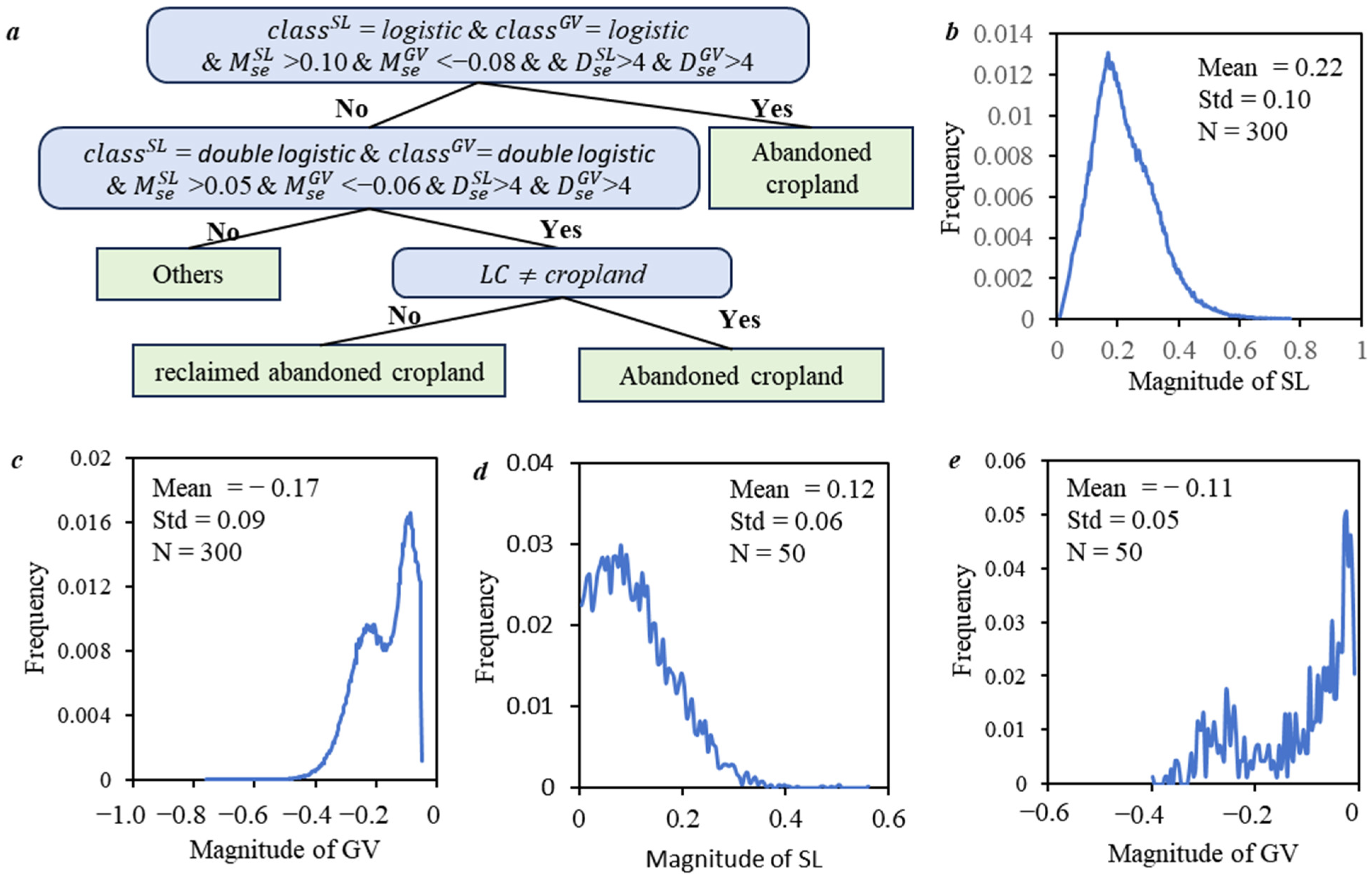
2.4.3. Detecting Cropland Abandonment Using Knowledge-Based Framework

A knowledge-based framework is used to identify cropland abandonment from interactive endmember fractions (Table 3 and Figure 5). In cases where the optimal result of the time series fitting is a logistic curve, cropland degradation and soil exposure can be inferred by examining the magnitude of vegetation and soil changes. Specifically, a negative vegetation change combined with a positive soil change indicates vegetation degradation and soil exposure during cropland abandonment (Figure 5a). To detect these changes, a predefined empirical threshold is applied to the magnitude of change, ensuring the robustness of this characterization. This threshold is defined as the difference between the mean and standard deviation of the histogram of the magnitude of change in SL/GV endmembers [29,33], derived from the interest area of cropland abandonment selected from Google Earth historical imagery (Figure 5b,c). When the time series fitting yields a double-logistic curve as the optimal result, cropland evolution exhibits more complex characteristics, encompassing three potential types: abandoned cropland, reclaimed abandoned cropland, and fallow cropland. Identifying areas of cropland abandonment requires the integration of land use/land cover data with spectral endmember time series curves to establish classification rules and delineate categories (Figure 5a). Initially, regions of potential cropland change are identified based on vegetation displaying a U-shaped curve and soil exhibiting an inverted U-shaped curve. Subsequently, areas undergoing fallow are excluded by applying the criterion requiring that the duration of the vegetation endmember’s trough or the soil endmember’s peak exceeds four years. Finally, abandoned cropland and reclaimed abandoned cropland are differentiated using post-change land cover types: if the subsequent land cover type is non-cropland, then the area is classified as abandoned cropland; otherwise, it is classified as reclaimed abandoned cropland. The threshold is also defined as the difference between the mean and standard deviation of the histogram of magnitude of change in SL/GV endmembers (Figure 5d,e). This dual framework provides a systematic approach to detecting and characterizing cropland abandonment dynamics, leveraging the temporal and spectral properties of endmember time series data.

2.4.4. Validation and Assessments

To validate the cropland abandonment detection results, we generated 200 random points for each detected type in the study area and traced their change pathways using historical images from Google Earth. Points with comprehensive and visual images during the study period were selected as the validation set and then classified as abandoned cropland, reclaimed abandoned cropland, and others. To ensure authenticity, we implemented a verification protocol. First, to confirm persistent abandonment/fallow patterns, the samples were tracked across ≥5 growing seasons. Second, two independent analysts classified all samples using high-resolution imagery. Third, samples with unresolved disagreements were excluded from accuracy calculations. Finally, highly feasible validation points (188 for abandoned cropland, 144 for reclaimed abandoned cropland, and 190 for others) were used to assess the robustness of our knowledge-driven framework.
Moreover, the widely used land cover-based detection method was also used to generate a map of cropland abandonment. This method uses annual land cover maps to identify cropland abandonment based on a rule of five consecutive years of non-cropland [23] (Tu et al., 2024). We thus used the China Annual Cropland Dataset at 30 m from 2000 to 2021 to generate maps of abandoned and reclaimed abandoned cropland.

3. Results

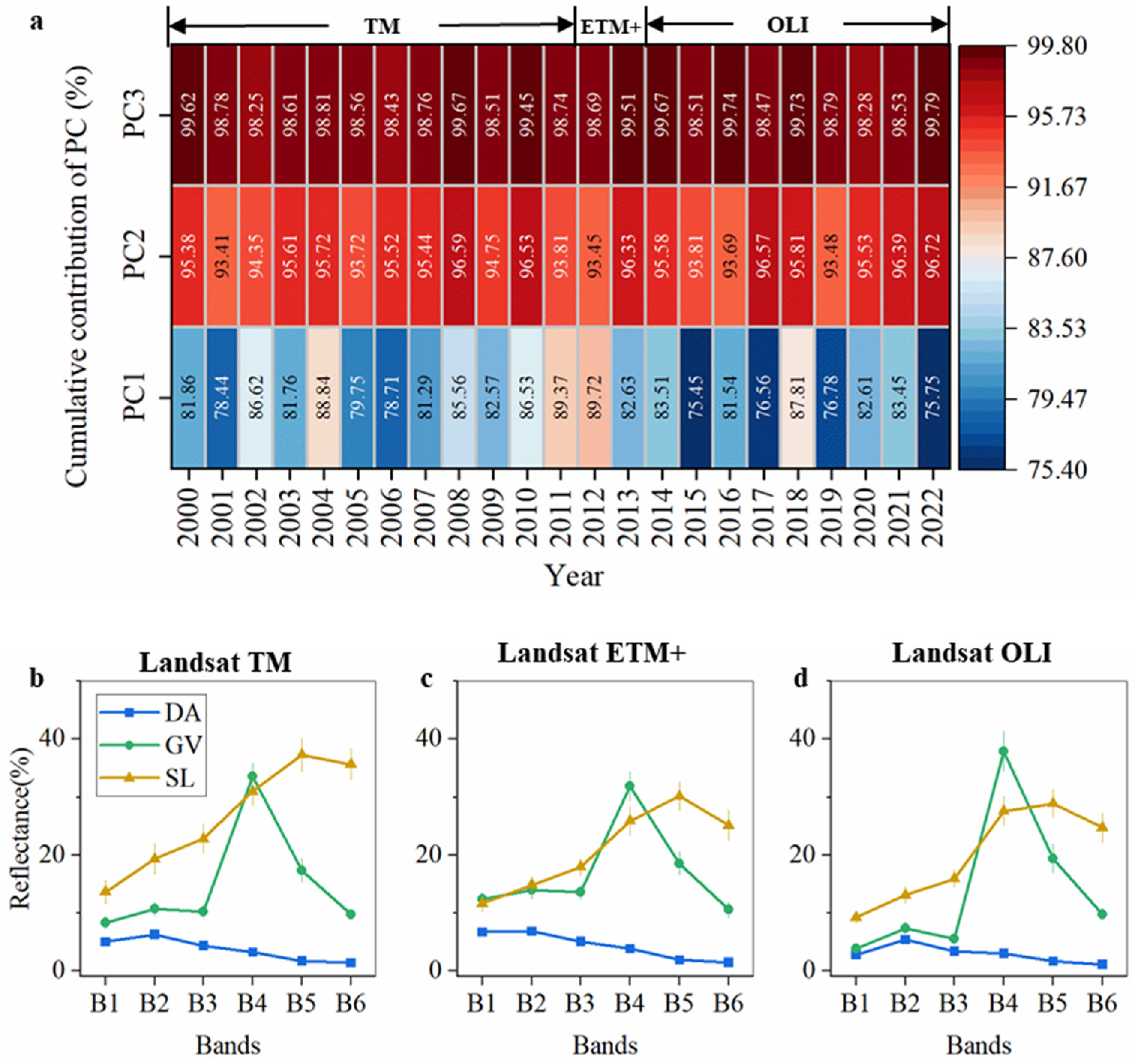
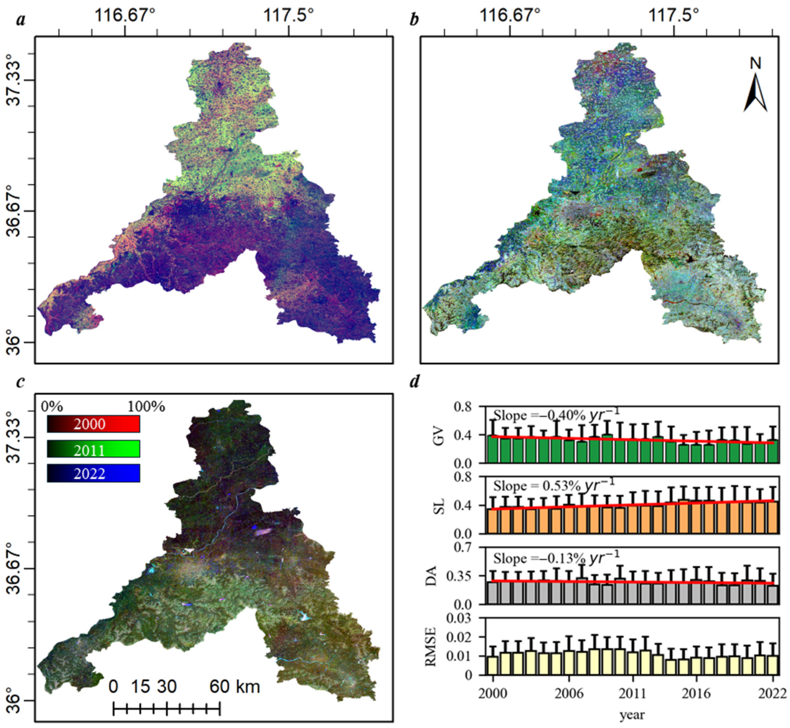
3.1. Annual Estimates of GV, SL, and DA Fractional Maps

The figure illustrates the temporal trends in the fractions of the three spectral endmembers—GV, SL, and DA—derived from spectral unmixing decomposition from 2000 to 2022, along with the root mean square error (RMSE) of the spectral mixture models (Figure 6). The RMSE values remain consistently low throughout the period (<2%), confirming the stability and reliability of the spectral unmixing process. The GV fraction time series shows a declining trend, with a slope of −0.40% per year, indicating a gradual reduction in vegetation cover over the study period. In contrast, the SL fraction time series increases at a rate of 0.53% per year, reflecting a possible expansion of exposed soil or urbanization processes. The DA abundance exhibits a slight decline, with a slope of −0.13% per year, suggesting marginal decreases in the proportion of dark surface materials. These trends collectively suggest significant land cover changes, with potential implications for vegetation loss and soil exposure dynamics over the study period.

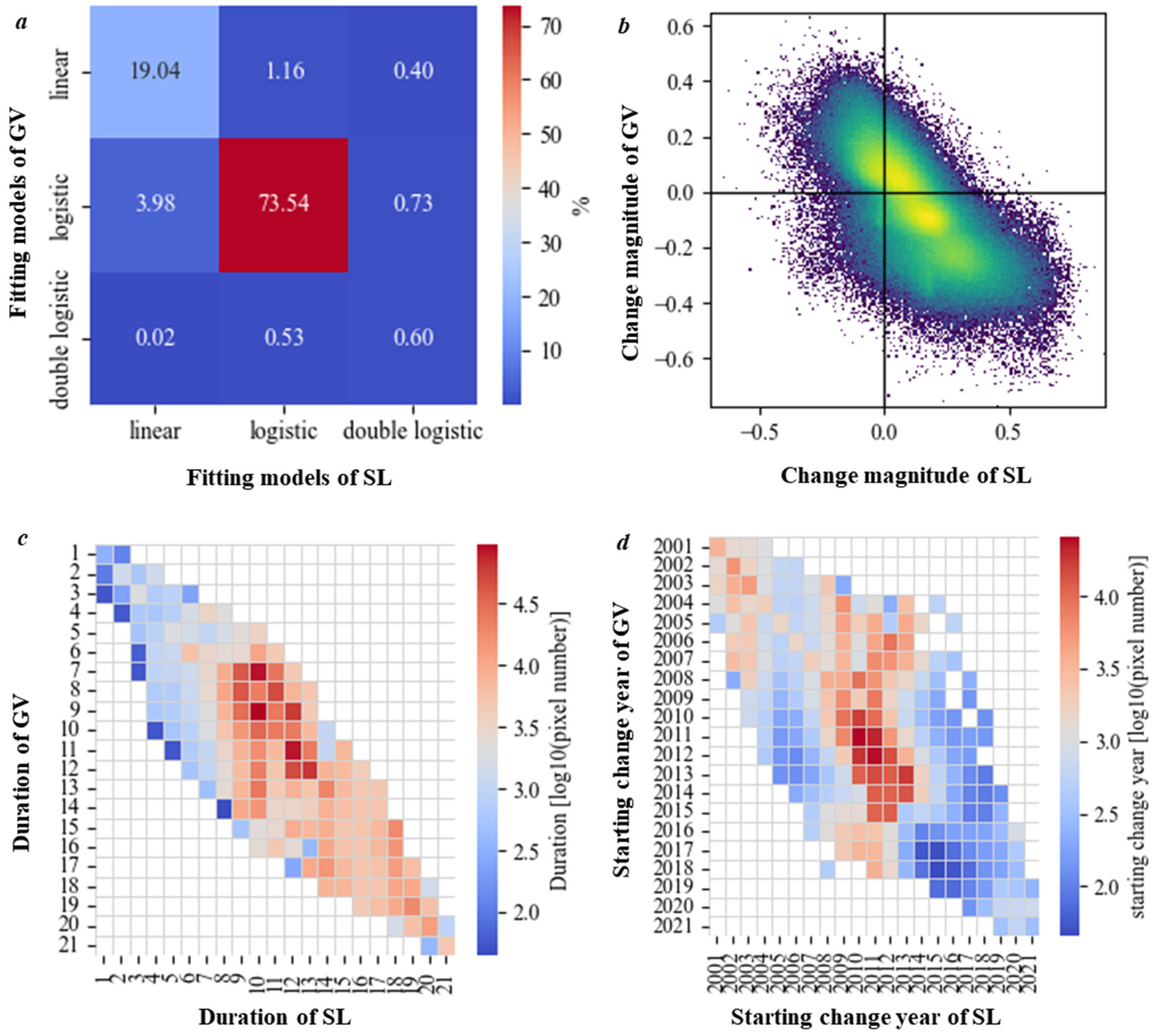
3.2. Multi-Dimensional Thematic Features in Vegetation–Soil Endmember Time Series

An analysis of the time series fitting of the GV and SL abundance values reveals distinct spatial and temporal patterns across the study area. The fitting models for GV and SL exhibit a relatively consistent spatial pattern (Figure 7a,e). The spatial distribution of the fitting models for both GV and SL shows a dominant presence of the logistic model, which characterizes 78.24% and 75.23% of the study area, respectively. This suggests that human activity dominated the temporal dynamics of both the GV and SL fractions. Another human activity-dominated type of double-logistic curve is mainly concentrated in certain areas (1.15% and 1.73%), indicating the discontinued use of cropland. There are relatively fewer linear changes than non-linear changes in the study area, accounting for only 20.60% and 23.04% of the GV and SL fraction time series (Figure 8a). The magnitude of change displays substantial variation across the study area. The areas fitted with the logistic model exhibit high change magnitudes for both GV and SL (Figure 7b,f).
Additionally, a strong negative correlation is observed between the change magnitudes of GV and SL, indicating that a significant increase in SL is closely linked to a decrease in GV. Furthermore, this trend of increasing SL and decreasing GV is the primary interaction type within the region (Figure 8b). We found that the duration and starting change year have a high degree of spatial consistency (Figure 7c,d,g,h). This phenomenon is also confirmed in Figure 8c,d, where the distribution of the duration for both SL and GV mainly falls between 8 and 15 years, and the starting change year is predominantly concentrated around 2010. The interrelationship between the fitting models, change magnitude, duration, and starting change year of GV and SL further indicates strong temporal coherence. Additionally, based on the available 23 points, a high degree of consistency is observed between the results of our model simulations and the turning times shown by Google Earth, with an RMSE close to 1 year (Figure S3). These findings highlight the dominant role of logistic growth patterns in shaping the temporal dynamics of both variables and underscore the interconnectedness of GV and SL abundance changes in the study area.

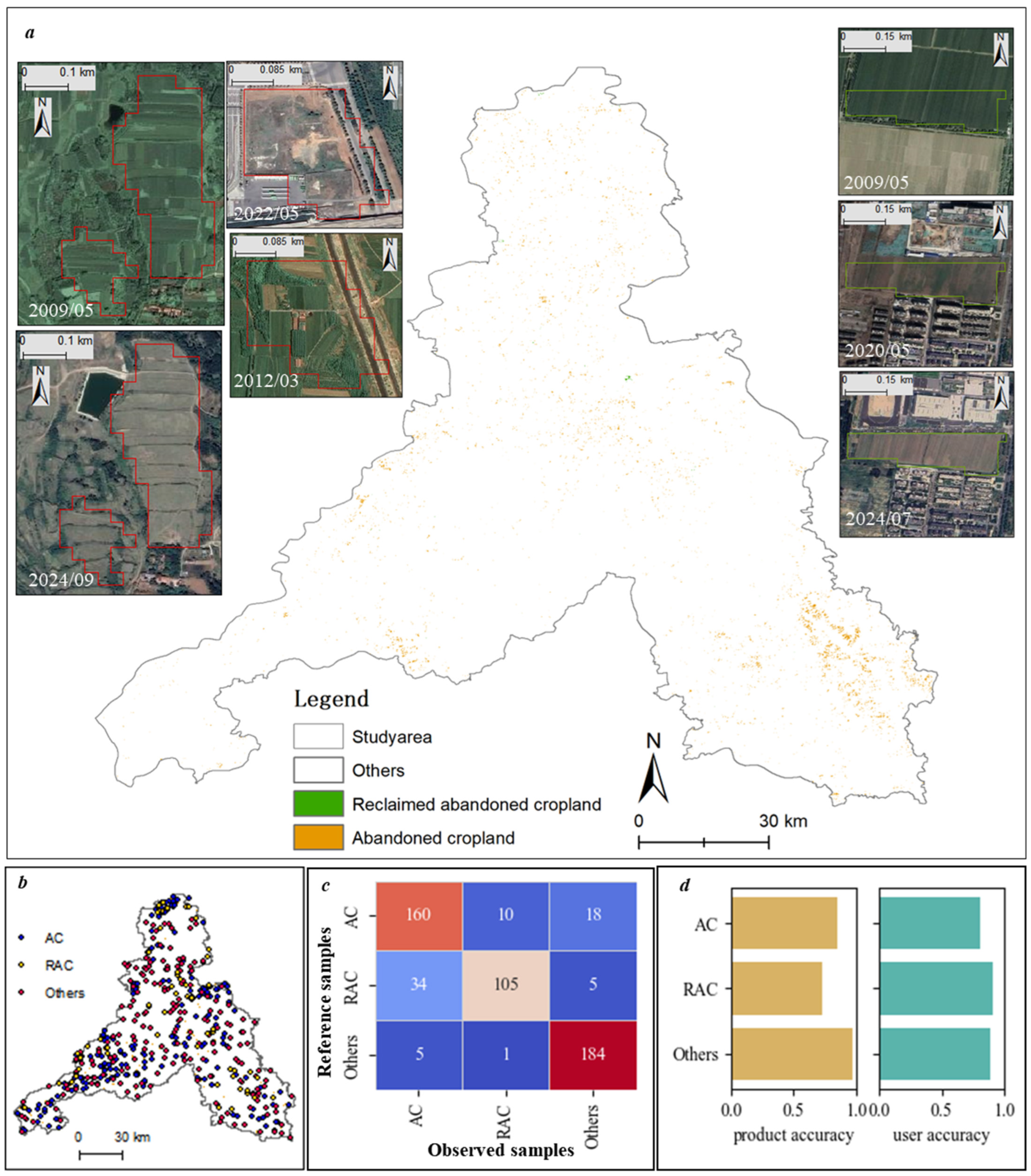
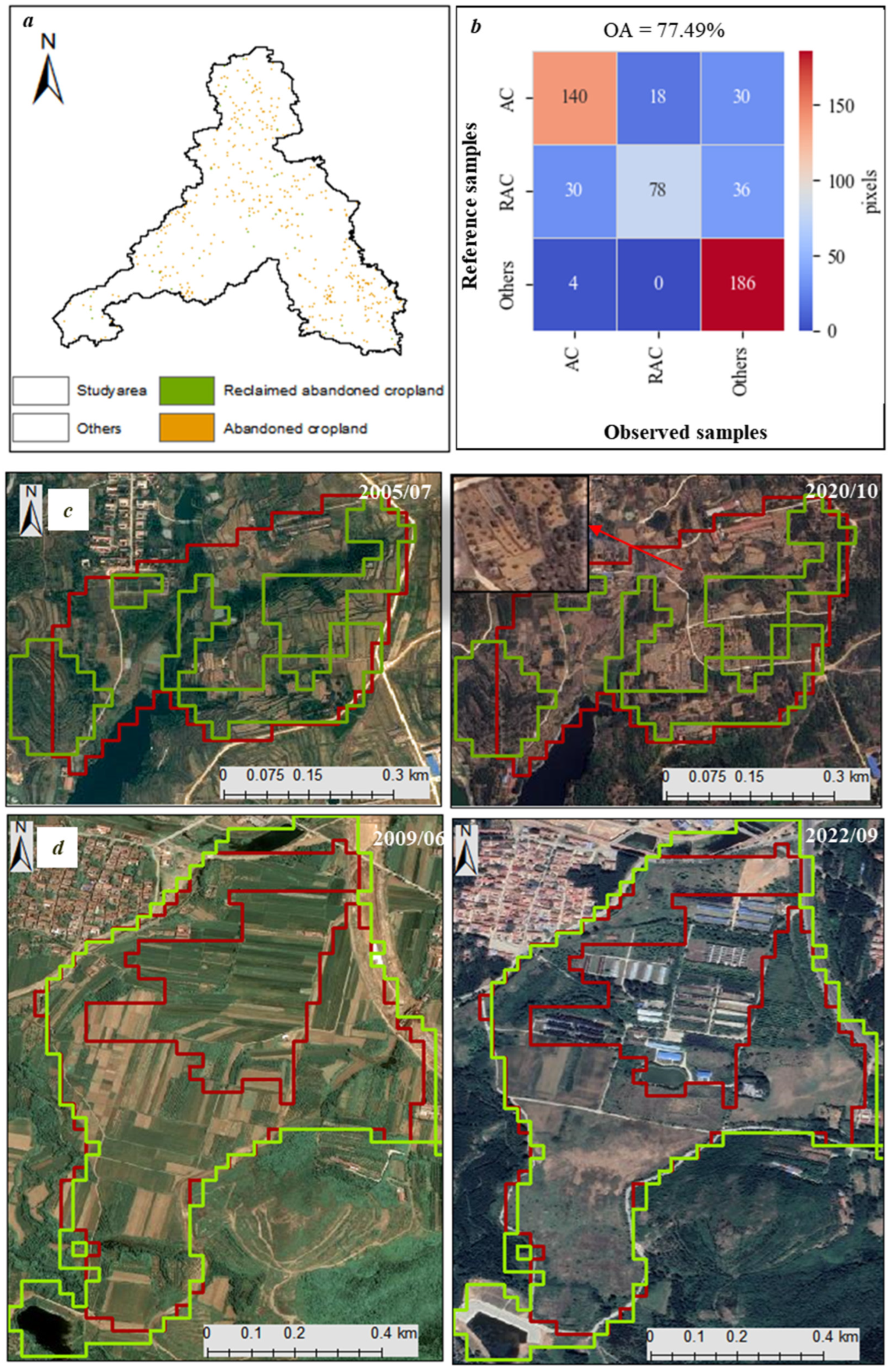
3.3. Mapping Cropland Abandonment: Abandoned vs. Reclaimed Cropland

The monitoring results for abandoned and reclaimed cropland classification are presented in Figure 9. The results revealed that abandoned cropland is scattered across the study area, with a notably higher concentration in the southern mountainous regions. Conversely, reclaimed abandoned cropland is relatively scarce and occurs only sporadically within the region. To further validate the classification, we overlaid the detection results onto Google Earth historical imagery. This overlay revealed that our method, through its accurate characterization of the interactive evolutionary features of multi-factor time series at various stages, effectively captures both the abandonment and reclamation processes of cropland (Figure 9a). The advantages of the proposed method are further validated by the accuracy assessment of the sample data, with an overall accuracy of 86.02% (Figure 9b–d). The accuracy of abandoned cropland detection was relatively high, with product accuracy exceeding 85%. However, the product accuracy for reclaimed abandoned cropland was lower at 72.92%. The primary source of error for reclaimed abandoned cropland detection was its misclassification as abandoned cropland, which can be attributed to the time series trend fitting model’s inadequate response to signals from late-stage reclamation, which were instead fitted into logical curves. This limitation of the model also resulted in a lower user accuracy for abandoned cropland detection, which was 80.40%. However, the user accuracy for reclaimed abandoned cropland was higher than 90%, reflecting a relatively low commission error for this type. Overall, the multi-factor time series trend fitting and feature extraction method demonstrates the potential for highly accurate cropland abandonment detection. The approach can effectively identify abandoned cropland while capturing reclamation dynamics with satisfactory precision.

4. Discussion

4.1. Comparison to Land Cover-Based Detection Methods

Land cover change-based cropland abandonment monitoring has been widely applied in various regions and is significant for monitoring cropland changes [6,34]. However, compared to the multi-factor time series fitting method proposed in this study, existing methods heavily rely on annual cropland cover maps and construction land data. This dependency can limit the monitoring accuracy of land cover change-based methods, as their precision is inherently constrained by the accuracy of the land cover data [19]. Although many cropland and land cover datasets have been released, their accuracy is usually just over 80% [35,36], which raises concerns regarding their reliability in cropland abandonment monitoring. The overall accuracy of land cover-based detection methods is 77.39%, which is inferior to that of our proposed framework (Figure 10a,b). Our method offers several advantages over traditional land cover change-based methods. First, it reduces errors when distinguishing cropland during the early stages of land transformation, particularly when large amounts of bare soil are present. Our method effectively captures this signal by monitoring the increase and reduction in soil and vegetation endmembers (Figure 10c). Furthermore, errors in land cover classification, often caused by spectral confusion (such as rural construction or greenhouses being classified as ecological land), lead to the misclassification of cropland abandonment (Figure 10d), while this can be effectively addressed using the soil and vegetation time series interaction in our method. In addition, our method is more accurate at detecting scattered pixel/patch changes, although this may lead to some “salt-and-pepper” noise in the results. Nevertheless, it is capable of accurately identifying changes in land cover dynamics, including small-scale alterations that may otherwise be overlooked using traditional approaches [28]. This is particularly beneficial when studying the impact of cropland abandonment on landscapes, as it enables the detection of subtle shifts in land cover that may be overlooked in traditional detection methods.
Additionally, although established time series methods such as CCDC and BFAST are excellent at identifying land cover changes [37,38], our approach focuses on the dynamic and multi-phase nature of cropland abandonment. By capturing early indicators, such as vegetation decline and soil exposure, as well as long-term stabilization, our method provides a more comprehensive view of abandonment dynamics.

4.2. Advantages and Limitations of Change Detection from Endmember Time Series

The proposed framework for cropland abandonment detection using fractional endmember time series modeling has several strengths. Change detection using endmember time series offers significant advantages in providing detailed insights into surface composition changes over time and enables a more nuanced understanding of land cover dynamics through the analysis of endmember signatures [19,39]. In this study, the framework’s emphasis on modeling the full life cycle of cropland abandonment, from early indicators to long-term stabilization, allows for a more nuanced understanding of the abandonment process. This is particularly important because cropland abandonment often involves a combination of vegetation decline, soil exposure, and recovery phases, which can vary significantly over time. By capturing these dynamic changes, the framework provides a more complete and accurate picture of abandonment than methods that focus only on immediate changes or late-stage processes. Additionally, a critical strength of the framework lies in its capacity to differentiate between fallow and abandoned cropland despite their spectral and temporal similarities. Fallow periods typically exhibit cyclical or short-term vegetation suppression, followed by rapid recovery (<5 year), whereas abandonment manifests as a prolonged vegetation decline or a gradual transition to non-agricultural land cover (e.g., shrub encroachment and soil exposure). The endmember time series analysis captures these divergent temporal patterns by quantifying (1) the persistence of vegetation suppression, (2) the magnitude and directionality of post-suppression vegetation recovery, and (3) the long-term stabilization of endmember fractions through multi-stage parameters of full-life-cycle modeling. This multi-temporal, process-oriented approach reduces reliance on single-date spectral thresholds, which are prone to misclassification under intermittent agricultural use. Moreover, our logistic and double-logistic models transcend generic curve fitting by explicitly encoding climate-driven divergence in abandonment pathways. As quantified in Table 3, the framework’s humidity adaptations can capture secondary succession through accelerated vegetation encroachment using the double-logistic model. Conversely, arid adaptations incorporate soil exposure persistence terms through the logistic model, reflecting suppressed ecological recovery. This climate-contextualized modeling resolves a key limitation in universal abandonment algorithms, which often fail to distinguish between humid zone recolonization pulses and arid zone land degradation cascades. Future work will establish a global climate parameterization atlas to enable a seamless, large-scale framework.
One of the major limitations of using endmember time series for change detection is the dependence on high-quality, cloud-free, and temporally consistent imagery [39]. In tropical regions where cloud cover is persistent, achieving a clear, cloud-free image for each time point may be challenging, potentially leading to gaps in the time series and unreliable change detection. However, the issue of endmember variability across regions has been widely recognized in remote sensing studies, as endmembers are often considered to be region-specific due to variations in vegetation types, soil composition, and other land cover characteristics [40]. Endmember selection uncertainty persists in rapid-transition landscapes, where spectral mixtures may alias abandonment signals. With the development of large-scale regional and global endmember abundance time series products, this challenge can be addressed in a more systematic and consistent manner [19]. Moreover, time series analysis involving the fitting of multiple models to large datasets can be computationally expensive. This can be a significant limitation when working with big data or in operational settings where rapid decision making is needed. While the framework improves the discrimination of fallow and abandoned cropland, challenges remain in regions where fallow cycles are exceptionally long, or abandonment coincides with rapid natural revegetation. In such cases, spectral–temporal signals may overlap significantly, necessitating integration with ancillary data (e.g., land use records and field surveys) to resolve uncertainties. Future work should explore hybrid approaches combining endmember time series with contextual features (e.g., parcel boundaries and proximity to infrastructure) to further enhance class separability. While our verification protocol strengthens validation sample reliability, regions lacking ground truth data (e.g., remote mountainous areas) remain dependent on visual interpretation. Future work should integrate crowd-sourced geo-tagged photos or UAV data to further reduce uncertainty. Additionally, although the histogram-based threshold determination method employed in this study (e.g., change magnitude = μ ± σ) is well established in the land change detection literature [28,33], we recognize its inherent regional dependency. Threshold determination under zonal control could be carried out in the future, contributing to wide-scale cropland abandonment.

5. Conclusions

In this study, we developed a novel framework for cropland abandonment detection by integrating the full-life-cycle modeling of vegetation–soil endmember time series derived from dense Landsat observations. Trends of a declining GV (−0.40% per year) and increasing SL (+0.53% per year) revealed the dominant pathways of vegetation degradation and soil exposure during abandonment. Spatially consistent durations (8–15 years) and initiation years (around 2010) further quantified the temporal patterns of abandonment, providing critical parameters for region-specific land management strategies. By reconstructing interactive trajectories of GV and SL fractions using logistic/double-logistic models, our framework achieved an overall accuracy of 86.02%, outperforming traditional land cover classification methods. This method effectively mitigates error propagation in multi-temporal classification and enhances sensitivity to fine-scale spatial changes (e.g., scattered abandonment patches). The framework successfully distinguished abandonment from reclamation and fallow scenarios in Jinan, China, demonstrating its robustness in capturing multi-stage interactions between natural recovery and human disturbances. This capability supports adaptive policymaking for sustainable agriculture and ecosystem restoration.

Supplementary Materials

The following supporting information can be downloaded at https://www.mdpi.com/article/10.3390/rs17132193/s1: Figure S1: Cropland boundaries overlaid on Google Earth images in 2000; Figure S2: Comparisons of RMSE and Bayesian Information Criterion for optimal fitting result selection for different series; Figure S3: Starting change point timing validation. Above is the selection of the validation sample points based on high spatial resolution Google Earth imagery of the historical period, and below is the scatter plot between change points from high spatial resolution images and starting change point timing; Table S1: Definitions of cropland for products used in this study.

Author Contributions

Conceptualization, Q.S., P.Z. and H.W.; methodology, Q.S. and Z.Y. (Zhijun You); software, Q.S.; validation, Q.S., Z.Y. (Zhijun You), Z.Y. (Zhonghai Yu) and L.W.; resources, Q.S. and H.W.; data curation, Z.Y. (Zhijun You); writing—original draft preparation, Q.S. and P.Z.; writing—review and editing, H.W., Z.Y. (Zhonghai Yu) and L.W.; visualization, Q.S. and P.Z.; funding acquisition, Q.S. and H.W. All authors have read and agreed to the published version of the manuscript.

Funding

This work was supported by the National Key R&D Program of China (grant no. 2023YFB3907600).

Data Availability Statement

The data and code can be requested from the authors.

Conflicts of Interest

The contact author has declared that none of the authors has any competing interests.

References

  1. Rey Benayas, J.M.; Martins, A.; Nicolau, J.M.; Schulz, J.J. Abandonment of agricultural land: An overview of drivers and consequences. CABI Rev. 2007, 57, 1–14. [Google Scholar] [CrossRef]
  2. Hong, C.; Prishchepov, A.V.; Bavorova, M. Cropland abandonment in mountainous China: Patterns and determinants at multiple scales and policy implications. Land Use Policy 2024, 145, 107292. [Google Scholar] [CrossRef]
  3. Crawford, C.L.; Wiebe, R.A.; Yin, H.; Radeloff, V.C.; Wilcove, D.S. Biodiversity consequences of cropland abandonment. Nat. Sustain. 2024, 7, 1596–1607. [Google Scholar] [CrossRef]
  4. Knoke, T.; Calvas, B.; Moreno, S.O.; Onyekwelu, J.C.; Griess, V.C. Food production and climate protection—What abandoned lands can do to preserve natural forests. Glob. Environ. Change 2023, 23, 1064–1072. [Google Scholar] [CrossRef]
  5. Yang, Y.; Hobbie, S.E.; Hernandez, R.R.; Fargione, J.; Grodsky, S.M.; Tilman, D.; Zhu, Y.-G.; Luo, Y.; Smith, T.M.; Jungers, J.M.; et al. Restoring abandoned farmland to mitigate climate change on a full earth. One Earth 2020, 3, 176–186. [Google Scholar] [CrossRef]
  6. Zheng, Q.; Ha, T.; Prishchepov, A.V.; Zeng, Y.; Yin, H.; Koh, L.P. The neglected role of abandoned cropland in supporting both food security and climate change mitigation. Nat. Commun. 2023, 14, 6083. [Google Scholar] [CrossRef]
  7. Hong, C.; Prishchepov, A.V.; Jin, X.; Han, B.; Lin, J.; Liu, J.; Ren, J.; Zhou, Y. The role of harmonized Landsat Sentinel-2 (HLS) products to reveal multiple trajectories and determinants of cropland abandonment in subtropical mountainous areas. J. Environ. Manag. 2023, 336, 117621. [Google Scholar] [CrossRef]
  8. Löw, F.; Prishchepov, A.V.; Waldner, F.; Dubovyk, O.; Akramkhanov, A.; Biradar, C.; Lamers, J.P.A. Mapping Cropland Abandonment in the Aral Sea Basin with MODIS Time Series. Remote Sens. 2018, 10, 159. [Google Scholar] [CrossRef]
  9. Ye, J.; Hu, Y.; Feng, Z.; Zhen, L.; Shi, Y.; Tian, Q.; Zhang, Y. Monitoring of Cropland Abandonment and Land Reclamation in the Farming–Pastoral Zone of Northern China. Remote Sens. 2024, 16, 1089. [Google Scholar] [CrossRef]
  10. Tamiminia, H.; Salehi, B.; Mahdianpari, M.; Quackenbush, L.; Adeli, S.; Brisco, B. Google Earth Engine for geo-big data applications: A meta-analysis and systematic review. ISPRS J. Photogramm. Remote Sens. 2020, 164, 152–170. [Google Scholar] [CrossRef]
  11. Dara, A.; Baumann, M.; Kuemmerle, T.; Pflugmacher, D.; Rabe, A.; Griffiths, P.; Hölzel, N.; Kamp, J.; Freitag, M.; Hostert, P. Mapping the timing of cropland abandonment and recultivation in northern Kazakhstan using annual Landsat time series. Remote Sens. Environ. 2018, 213, 49–60. [Google Scholar] [CrossRef]
  12. Guo, A.; Yue, W.; Yang, J.; Xue, B.; Xiao, W.; Li, M.; He, T.; Zhang, M.; Jin, X.; Zhou, Q. Cropland abandonment in China: Patterns, drivers, and implications for food security. J. Clean. Prod. 2023, 418, 138154. [Google Scholar] [CrossRef]
  13. Long, Y.; Sun, J.; Wellens, J.; Colinet, G.; Wu, W.; Meersmans, J. Mapping the Spatiotemporal Dynamics of Cropland Abandonment and Recultivation across the Yangtze River Basin. Remote Sens. 2024, 16, 1052. [Google Scholar] [CrossRef]
  14. Hong, C.; Prishchepov, A.V.; Jin, X.; Zhou, Y. Mapping cropland abandonment and distinguishing from intentional afforestation with Landsat time series. Int. J. Appl. Earth Obs. Geoinf. 2024, 127, 103693. [Google Scholar] [CrossRef]
  15. Yin, H.; Brandão, A., Jr.; Buchner, J.; Helmers, D.; Iuliano, B.G.; Kimambo, N.E.; Lewińska, K.E.; Razenkova, E.; Rizayeva, A.; Rogova, N.; et al. Monitoring cropland abandonment with Landsat time series. Remote Sens. Environ. 2020, 246, 111873. [Google Scholar] [CrossRef]
  16. Elmore, A.J.; Mustard, J.F.; Manning, S.J.; Lobell, D.B. Quantifying vegetation change in semiarid environments: Precision and accuracy of spectral mixture analysis and the normalized difference vegetation index. Remote Sens. Environ. 2000, 73, 87–102. [Google Scholar] [CrossRef]
  17. Weng, Q.; Hu, X.; Liu, H. Estimating impervious surfaces using linear spectral mixture analysis with multitemporal ASTER images. Int. J. Remote Sens. 2009, 30, 4807–4830. [Google Scholar] [CrossRef]
  18. Sun, Q.; Zhang, P.; Wei, H.; Liu, A.; You, S.; Sun, D. Improved mapping and understanding of desert vegetation-habitat complexes from intraannual series of spectral endmember space using cross-wavelet transform and logistic regression. Remote Sens. Environ. 2020, 236, 111516. [Google Scholar] [CrossRef]
  19. Sun, Q.; Zhang, P.; Jiao, X.; Lin, X.; Duan, W.; Ma, S.; Pan, Q.; Chen, L.; Zhang, Y.; You, S.; et al. A global estimate of monthly vegetation and soil fractions from spatio-temporally adaptive spectral mixture analysis during 2001–2022. Earth Syst. Sci. Data Discuss. 2023, 16, 1333–1351. [Google Scholar] [CrossRef]
  20. Zhu, Z.; Wang, S.; Woodcock, C.E. Improvement and expansion of the Fmask algorithm: Cloud, cloud shadow, and snow detection for Landsats 4–7, 8, and Sentinel 2 images. Remote Sens. Environ. 2015, 159, 269–277. [Google Scholar] [CrossRef]
  21. Potapov, P.; Turubanova, S.; Hansen, M.C.; Tyukavina, A.; Zalles, V.; Khan, A.; Song, X.-P.; Pickens, A.; Shen, Q.; Cortez, J. Global maps of cropland extent and change show accelerated cropland expansion in the twenty-first century. Nat. Food 2022, 3, 19–28. [Google Scholar] [CrossRef] [PubMed]
  22. Oliphant, A.; Thenkabail, P.; Teluguntla, P. Global Food-Security-Support-Analysis Data at 30-m Resolution (GFSAD30) Cropland-extent Products—Download Analysis; U.S. Geological Survey Open-File Report 2022–1001; US Geological Survey: Reston, VA, USA, 2022; 20p. [CrossRef]
  23. Tu, Y.; Wu, S.; Chen, B.; Weng, Q.; Bai, Y.; Yang, J.; Yu, L.; Xu, B. A 30 m annual cropland dataset of China from 1986 to 2021. Earth Syst. Sci. Data 2024, 16, 2297–2316. [Google Scholar] [CrossRef]
  24. Chen, J.; Chen, J.; Liao, A.; Cao, X.; Chen, L.; Chen, X.; He, C.; Han, G.; Peng, S.; Lu, M.; et al. Global land cover mapping at 30 m resolution: A POK-based operational approach. ISPRS J. Photogramm. Remote Sens. 2015, 103, 7–27. [Google Scholar] [CrossRef]
  25. Zhang, X.; Zhao, T.; Xu, H.; Liu, W.; Wang, J.; Chen, X.; Liu, L. GLC_FCS30D: The first global 30 m land-cover dynamics monitoring product with a fine classification system for the period from 1985 to 2022 generated using dense-time-series Landsat imagery and the continuous change-detection method. Earth Syst. Sci. Data 2024, 16, 1353–1381. [Google Scholar] [CrossRef]
  26. Xu, X.; Li, B.; Liu, X.; Li, X.; Shi, Q. Mapping annual global land cover changes at a 30 m resolution from 2000 to 2015. Natl. Remote Sens. Bull. 2021, 25, 1896–1916. [Google Scholar] [CrossRef]
  27. Yang, J.; Huang, X. The 30 m annual land cover dataset and its dynamics in China from 1990 to 2019. Earth Syst. Sci. Data 2021, 13, 3907–3925. [Google Scholar] [CrossRef]
  28. Sun, D. Detection of dryland degradation using Landsat spectral unmixing remote sensing with syndrome concept in Minqin County, China. Int. J. Appl. Earth Obs. Geoinf. 2015, 41, 34–45. [Google Scholar] [CrossRef]
  29. Sun, Q.; Zhang, P.; Jiao, X.; Han, W.; Sun, Y.; Sun, D. Identifying and understanding alternative states of dryland landscape: A hierarchical analysis of time series of fractional vegetation-soil nexuses in China’s Hexi Corridor. Landsc. Urban Plan. 2021, 215, 104225. [Google Scholar] [CrossRef]
  30. Powell, R.L.; Roberts, D.A.; Dennison, P.E.; Hess, L.L. Sub-pixel mapping of urban land cover using multiple endmember spectral mixture analysis: Manaus, Brazil. Remote Sens. Environ. 2007, 106, 253–267. [Google Scholar] [CrossRef]
  31. Small, C.; Milesi, C. Multi-scale standardized spectral mixture models. Remote Sens. Environ. 2013, 136, 442–454. [Google Scholar] [CrossRef]
  32. Zhang, P.; Kohli, D.; Sun, Q.; Zhang, Y.; Liu, S.; Sun, D. Remote sensing modeling of urban density dynamics across 36 major cities in China: Fresh insights from hierarchical urbanized space. Landsc. Urban Plan. 2020, 203, 103896. [Google Scholar] [CrossRef]
  33. Li, X.; Zhou, Y.; Zhu, Z.; Liang, L.; Yu, B.; Cao, W. Mapping annual urban dynamics (1985–2015) using time series of Landsat data. Remote Sens. Environ. 2018, 216, 674–683. [Google Scholar] [CrossRef]
  34. Wu, X.; Zhao, N.; Wang, Y.; Ye, Y.; Wang, W.; Yue, T.; Zhang, L.; Liu, Y. The potential role of abandoned cropland for food security in China. Resour. Conserv. Recycl. 2025, 212, 108004. [Google Scholar] [CrossRef]
  35. Yadav, K.; Congalton, R.G. Accuracy Assessment of Global Food Security-Support Analysis Data (GFSAD) Cropland Extent Maps Produced at Three Different Spatial Resolutions. Remote Sens. 2018, 10, 1800. [Google Scholar] [CrossRef]
  36. Zhang, C.; Dong, J.; Ge, Q. Quantifying the accuracies of six 30-m cropland datasets over China: A comparison and evaluation analysis. Comput. Electron. Agric. 2022, 197, 106946. [Google Scholar] [CrossRef]
  37. Zhu, Z.; Woodcock, C.E. Continuous change detection and classification of land cover using all available Landsat data. Remote Sens. Environ. 2014, 144, 152–171. [Google Scholar] [CrossRef]
  38. Verbesselt, J.; Hyndman, R.; Newnham, G.; Culvenor, D. Detecting trend and seasonal changes in satellite image time series. Remote Sens. Environ. 2010, 114, 106–115. [Google Scholar] [CrossRef]
  39. Wang, Q.; Ding, X.; Tong, X.; Atkinson, P.M. Spatio-temporal spectral unmixing of time-series images. Remote Sens. Environ. 2021, 259, 112407. [Google Scholar] [CrossRef]
  40. Somers, B.; Asner, G.P.; Tits, L.; Coppin, P. Endmember variability in spectral mixture analysis: A review. Remote Sens. Environ. 2011, 115, 1603–1616. [Google Scholar] [CrossRef]
Figure 1. Technical framework of the full-life-cycle modeling of fractional endmember time series for cropland abandonment detection. GV and SL are the green vegetation and soil endmembers. (a) Illustration of the abandonment process using two interactive endmembers; (b) Technical process for detecting cropland abandonment.
Remotesensing 17 02193 g001
Figure 2. Study area of Jinan, Shandong Province. The neutral background image was sourced from World Terrain Base, produced by Esri, USGS, NOAA. The red box in the left panel represents the latitude and longitude range of the study area.
Remotesensing 17 02193 g002
Figure 3. Spectral curves of specific endmembers for Landsat. (a) Cumulative contributions of the first three principal components. (bd) Mean and standard deviation of the spectral curves for the three surface endmembers, namely SL, GV, and DA, which represent green vegetation, soil, and dark material, for three Landsat sensors, TM (b), ETM+ (c), and OLI (d). B1–B6 are the blue, green, red, near-infrared, short-wave infrared 1, and short-wave infrared 2 bands.
Remotesensing 17 02193 g003
Figure 4. Change points detected through second derivative of logistic modeling. The left plane is a schematic of a logistic curve, while the right plane is a schematic of a double-logistic curve. The black dot line is change points for logistic and double-logistic curve.
Remotesensing 17 02193 g004
Figure 5. A knowledge-based framework used to identify cropland abandonment. (a) Decision tree for abandoned cropland and reclaimed abandoned cropland identification. Class represents the type of curve fit, and M s e and D s e represent the magnitude and duration of the fitted curve, respectively (see Table 2 for details on the meaning of the different fitting types). LC is the land cover type at the end of the period. The superscripts of the parameters represent the different end-element types. (b,c) Histogram of the magnitude of change in SL and GV endmembers derived from the interest area of cropland abandonment selected from Google Earth historical imagery, respectively. (d,e) Histogram of the magnitude of change in SL and GV endmembers derived from the interest area of reclaimed abandoned cropland and natural vegetation-covered abandoned cropland selected from Google Earth historical imagery, respectively.
Remotesensing 17 02193 g005
Figure 6. Estimates of three endmember fractions. (ac) False-color composite image of multi-year fractional endmembers for GV, SL, and DA, respectively. Red, green, and blue represent 2000, 2011, and 2022. (d) Average and temporal trends in the fractions of the three endmembers, expressed through the slope of the linear regression (red lines).
Remotesensing 17 02193 g006
Figure 7. Parameters for fitting the GV and SL fraction time series. (a,e) Spatial distribution of fitting models for GV and SL masked by non-cropland. (b,f) The change magnitudes of GV and SL masked by non-cropland. (c,g) The change duration of logistic and double-logistic models. (d,h) Starting change point timing of GV and SL masked by non-cropland and the zone of fitted linear models.
Remotesensing 17 02193 g007
Figure 8. Relationship of fitted parameters between GV and SL series. (a) Heatmap of the confusion matrix used to represent the spatial correspondence between the GV and SL time series fit model types. (b) Scatter density plots used to represent the spatial correspondence between the magnitude of changes in the GV and SL time series, where blue to yellow represents an increase in scatter density. (c,d) Two-dimensional histograms (the size of the bin is 1 year) representing the relationship between the duration and starting change year of GV and SL, respectively.
Remotesensing 17 02193 g008
Figure 9. Monitoring results for abandoned and reclaimed cropland. (a) Spatial distribution of abandoned cropland and reclaimed abandoned cropland with overlaid Google Earth historical imagery. The red border is the extension where we have detected abandonment of cropland. (b) Randomly generated validation samples (200 of each type). (c) Confusion matrix generated after determination using Google Earth historical imagery. (d) Product and user accuracy of monitoring results. AC and RAC are abandoned cropland and reclaimed abandoned cropland, respectively.
Remotesensing 17 02193 g009
Figure 10. Comparison to land cover-based detection methods. (a) Spatial distribution of abandoned and reclaimed abandoned cropland using traditional land cover change-based methods. (b) Confusion matrix generated after determination using Google Earth historical imagery. (c,d) Result comparison between our framework (red boundary) and land cover-based detection methods (green boundary), with overlaid Google Earth historical imagery. Red arrow in the right panel of (b) represent a zoomed-in image of a typical area. AC and RAC are abandoned cropland and reclaimed abandoned cropland, respectively.
Remotesensing 17 02193 g010
Table 1. Global cropland and land cover monitoring datasets.
ProductsSpatial ResolutionTime SpanDeclared AccuracySource
Global Cropland Change 2000–201930 m2000–2019OA: 97.5%[21]
GFSAD30 m2000–2020OA: 91.7%[22]
CACD30 m1986–2021OA: 93%[23]
Globeland3030 m2000/2010/2020OA: 83.5–85.7%
PA of cropland: 79.6%
[24]
GLC_FCS30D30 m1985–2022OA: 80.88%
PA of cropland: 87.22%
[25]
AGLC30 m2000–2015OA: 76.10%
PA of cropland: 74.23%
[26]
CLCD30 m1990–2019OA: 79.30%
PA of cropland: 71.43–86.22%
[27]
Table 2. Parameters of optimal fitting models.
Fitting ModelParametersExplanations
LinearkChange magnitude from 2001 to 2022
Logistic T s Starting change point timing
T e Ending change point timing
M s e Change magnitude from starting point to ending point
D s e Duration between 2022 and starting change point timing
Double-logistic T s 1 Starting change point timing for first logistic
T e 1 Ending change point timing for first logistic
M s e Change magnitude for ending change point timing for first logistic and Starting change point timing for second logistic
T s 2 Starting change point timing for second logistic
T e 2 Ending change point timing for second logistic
D s e Duration between ending change point timing for first logistics and starting change point timing for second logistics
Table 3. Scenario knowledge and key points of identification from interactive time series of vegetation and soil fractions.
Scenario TypeScenario KnowledgeSchematic of the Time SeriesEssentials for Identification
Abandoned croplandIn arid zones, cropland abandonment leads to a sharp decrease in GV, accompanied by an increase in SL. Due to water constraints, most of the cropland after abandonment is dominated by bare soil or low-cover barren land.Remotesensing 17 02193 i001
Time series of vegetation and soil fractions are consistent with logistic regression.
The magnitude of change is negative for vegetation and positive for soil.
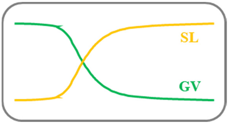
In humid zones, cropland abandonment also results in a sharp decrease in GV, accompanied by an increase in SL. However, natural vegetation gradually recovers, and natural land types with a high degree of cover are dominant after the abandonment of cultivated land.
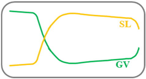
Remotesensing 17 02193 i002
Vegetation and soil fraction time series are consistent with double-logistic regression.
The magnitude of change is negative for vegetation and positive for soil.
Later land cover types are natural vegetation.
Reclaimed croplandInitially, the abandonment of cropland leads to a sharp reduction in vegetation cover, accompanied by an increase in bare soil, which again develops as cropland land after a sustained period of natural land cover (≥5 years).Remotesensing 17 02193 i003
Vegetation and soil fraction time series are consistent with double-logistic regression.
Later land cover type is cropland.
Distinguished from fallow by the criterion of no less than 5 years in a relatively steady period.
Disclaimer/Publisher’s Note: The statements, opinions and data contained in all publications are solely those of the individual author(s) and contributor(s) and not of MDPI and/or the editor(s). MDPI and/or the editor(s) disclaim responsibility for any injury to people or property resulting from any ideas, methods, instructions or products referred to in the content.

