Mechanisms Driving the Nonlinear Relationship Between Soil Freeze–Thaw Cycles and NDVI from Remotely Sensed Data in the Eastern Tibetan Plateau

Abstract

Climate warming leads to earlier onset and shortened duration of the freeze–thaw period in the eastern Tibetan Plateau, which has complex effects on vegetation growth. We assessed the spatiotemporal changes in the freeze–thaw period, evaluated its relationship with Normalized Difference Vegetation Index (NDVI from remotely sensed data), used the Panel Smooth Threshold Regression (PSTR) model to quantify the nonlinear impacts and identify critical thresholds, and applied ridge regression to explore the dominant mechanisms under different climatic conditions. The results showed the following: (1) The duration of the freeze–thaw transition period showed strong latitudinal zonality, with stronger spring disturbances than autumn ones. The trend of soil freeze–thaw status in high-altitude areas is the most significant, with a significant increase in the complete thaw period (CTP) and a significant decrease in the complete freeze period (CFP). (2) The earlier onset of the spring freeze–thaw period (SFTTP) and the CTP benefits vegetation growth in both early and late seasons. The delayed autumn freeze–thaw period (AFTTP) benefits early-season vegetation growth but is less favorable for late-season growth. The delayed CFP is beneficial for vegetation growth throughout the year. (3) The CTP’s boost to NDVI collapses at an onset date of 110 days and duration of 190 days. The AFTTP’s benefit peaks at an onset date of 300 days. (4) Temperature and the CTP are key drivers of NDVI changes, especially in the mid-to-late growing season. Arid areas respond strongly to freeze–thaw disturbances, while moderate precipitation areas are less affected. This study is the first to quantitatively analyze the nonlinear mechanism of the freeze–thaw–vegetation relationship, offering a new theoretical basis.

1. Introduction

Freeze–thaw cycles are a key process in alpine ecosystems, affecting soil temperature [1,2], moisture dynamics [3,4], and vegetation growth [5,6]. In high-altitude areas, the freeze–thaw disturbances can supply moisture for vegetation growth [7,8] and also regulate soil structure and the rhizosphere environment, thereby influencing vegetation growth [9,10]. The physical and chemical properties of soil are altered during freeze–thaw processes, which have profound effects on vegetation growth [1,11]. The relationship between freeze–thaw processes and vegetation is not a simple linear one, but rather has complex nonlinear characteristics. These nonlinear characteristics can be seen in the following aspects: Firstly, the impact of freeze–thaw processes on vegetation has distinct seasonality [12]. For example, during the freeze–thaw transition period, spring freeze–thaw transition period (SFTTP) promotes vegetation growth by providing moisture [4], while autumn freeze–thaw transition period (AFTTP) inhibits vegetation growth due to low temperatures [13]. Freeze–thaw cycles can extend the growing season by altering soil temperature and moisture dynamics [14,15,16], but earlier thawing also increases the risk of late frost damage to vegetation [17,18]. The complete thaw period (CTP) may promote vegetation growth by increasing soil temperature, improving soil aeration, and enhancing nutrient supply [11,19,20], but it can also lead to soil moisture loss [21]. The complete freeze period (CFP) may suppress vegetation growth by lowering soil temperature [22], but it can also maintain soil moisture by reducing soil evaporation, thereby promoting vegetation growth [23]. Secondly, the impact of freeze–thaw processes has threshold and lag effects [22,24]. Studies have found that freeze–thaw actions can release large amounts of carbon and nutrients from soil and microorganisms into the soil solution, providing short-term nutrient support [25], but they also affect soil aggregate stability and plant roots [26,27,28]. Soil respiration significantly increases after freeze–thaw cycles, enhancing nutrient release [29,30], but this increase gradually weakens as the number of freeze–thaw cycles increases [31]. Meanwhile, laboratory studies have shown that freeze–thaw cycles change microbial communities and functions, leading to higher nitrogen transformation rates in the next growing season [32] and significantly increased early-season vegetation productivity [33]. Thirdly, the impact of freeze–thaw processes is also regulated by climatic factors [34,35,36]. Existing studies indicate that temperature and precipitation affect the intensity and frequency of freeze–thaw processes [1], and freeze–thaw cycles can influence vegetation growth by affecting the sensitivity of vegetation to climatic factors [14].

Analyzing the impact of freeze–thaw processes on vegetation through linear regression methods has laid an important foundation for understanding the relationship between freeze–thaw processes and vegetation [37,38,39,40,41,42,43,44]. However, linear models assume that the relationship between variables remains constant over the entire range, which does not align with the actual situation. During the soil freeze–thaw process, the response of vegetation to soil freeze–thaw status may vary significantly across different threshold intervals, a difference that linear models fail to reflect. Among common nonlinear models, Generalized Additive Models (GAM) can flexibly capture the nonlinear relationships between variables [45], but they have poor model interpretability. Geographically Weighted Regression (GWR) models can capture spatial heterogeneity in geographical data [46], but they require high quality and density of spatial data. Wavelet Analysis can capture multi-scale features [47], but it is sensitive to the choice of wavelet basis functions. Machine learning models (such as random forests, support vector machines, etc.) can automatically learn complex nonlinear relationships [48], but they also have poor model interpretability. Given these limitations, this study opts for the Panel Smooth Threshold Regression (PSTR) model to explore the nonlinear relationship between soil freeze–thaw status and Normalized Difference Vegetation Index (NDVI). The PSTR model can fully exploit the structural features of panel data, taking into account both the differences among cross-sectional individuals and the dynamic changes in time series [49]. Additionally, the PSTR model introduces a smooth threshold transition mechanism, which can better reflect the nonlinear relationships between variables, thus avoiding model instability and estimation bias caused by the discontinuity of thresholds. This study aims to explore the impact mechanisms of freeze–thaw processes on vegetation through the PSTR method, especially the threshold and lag effects, thereby providing a scientific basis for the management and protection of alpine ecosystems.

In existing studies, the impact of freeze–thaw cycles on vegetation mainly includes direct and indirect effects. Direct effects consist of the promotion of vegetation by permafrost degradation and meltwater supply [50,51,52,53], as well as the inhibition of vegetation growth due to root damage [5]. Indirect effects include the influence of soil freeze–thaw on soil physical properties (such as soil structure affecting water infiltration and aeration) [54,55] and chemical properties (such as microbial activity influencing nutrient cycling) [56], thereby indirectly affecting the growth conditions of vegetation and the stability of ecosystems. From a temporal perspective, the impact of freeze–thaw cycles on vegetation can be further divided into short-term and long-term effects. Short-term effects are primarily the physical damage to soil and vegetation caused by freeze–thaw cycles [57]; long-term effects include the extension of the growing season [14], improvement of soil structure [11], increase in nutrient supply [2], and changes in microbial community functions [58,59]. However, current research has not yet quantified the temporal effects of freeze–thaw frequency, intensity, and duration on vegetation growth. Moreover, existing studies have mainly focused on permafrost regions, while research on the vegetation response mechanisms in seasonally frozen soil areas is insufficient. The freeze–thaw dynamics in seasonally frozen soil areas are significantly different from the soil degradation in permafrost regions [60,61,62], and thus, more in-depth studies targeting seasonally frozen soil areas are needed. More importantly, existing studies often use linear methods, which fail to identify the nonlinear impacts in the freeze–thaw–vegetation relationship, leading to an insufficient understanding of the threshold effects in this relationship. Nonlinearity is one of the keys to understanding the freeze–thaw–vegetation relationship. Therefore, it is necessary to introduce a nonlinear analysis method to reveal the nonlinear impact mechanisms of freeze–thaw processes on vegetation.

The eastern Tibetan Plateau is a transitional zone between permafrost and seasonally frozen soil, characterized by intense freeze–thaw disturbances and an ecosystem that is highly sensitive to environmental changes [63,64]. This region is not only an important component of the Asian water tower (Figure 1), but its ecological changes also have significant impacts on regional hydrology, carbon cycling, and climate feedback [65,66,67]. In recent years, with climate warming, the eastern Tibetan Plateau has experienced a shortened duration of freezing, an earlier onset of thawing, and an increased intensity of melting. These changes may have more complex impacts on vegetation. However, the response mechanisms of vegetation to different freeze–thaw stages are still unclear. How climatic factors regulate the freeze–thaw–vegetation relationship and whether there are dominant variables remain unanswered questions. Therefore, it is necessary to systematically analyze the regulatory role of climatic factors in the freeze–thaw–vegetation relationship to reveal the impact mechanisms of freeze–thaw processes on vegetation.

Based on the above analysis, this study aims to (1) reveal the nonlinear characteristics of the freeze–thaw–vegetation relationship in the eastern Tibetan Plateau, identify critical thresholds, and analyze the lag effects of vegetation in response to freeze–thaw changes. (2) Explore the key controlling factors of ecological processes by analyzing the mechanisms through which different freeze–thaw stages affect vegetation. To achieve these goals, this study will first use remote sensing data and ground observation data to analyze the spatiotemporal characteristics of the freeze–thaw process in the eastern Tibetan Plateau. Then, the Panel Smooth Threshold Regression (PSTR) model will be employed to quantify the nonlinear impact of the freeze–thaw process on vegetation growth and identify the critical thresholds of the onset dates and distribution days of different freeze–thaw periods on vegetation growth. Finally, by integrating temperature and precipitation data, the regulatory role of climatic factors in the freeze–thaw–vegetation relationship will be analyzed to reveal the impact mechanisms of the freeze–thaw process on vegetation. (Technology roadmap for this study: Figure 2).

2. Data and Methods

2.1. Spatial Distribution and Temporal Trends of Soil Freeze–Thaw

To determine the soil freeze–thaw status, this paper selects the ERA5-LAND reanalysis dataset provided by the European Centre for Medium-Range Weather Forecasts (ECMWF), which has an hourly temporal resolution and a 0.1° spatial resolution, covering the time period from 1950 to 2024 (https://cds.climate.copernicus.eu/, accessed on 25 April 2025). In this study, hourly surface temperature data from the ERA5-LAND dataset for the eastern Tibetan Plateau from 1 January 1982 to 31 December 2022 are used. Following the methodology of Shan et al. [68], we select shallow-layer (0–7 cm) soil temperature data, which is close to the 0 cm surface temperature data, for the study of near-surface soil freeze–thaw status.

Based on the hourly soil temperature data for the 0–7 cm layer in NetCDF format, we used Python 3.12 to statistically derive the daily maximum and minimum surface temperature data from 1982 to 2022. Subsequently, the aforementioned data were subjected to projection transformation and data clipping, uniformly employing the WGS 1984 geographic coordinate system and the Albers Equal Area Conic projection, with the central meridian at 110°E and standard parallels at 25°N and 47°N. Considering the significant topographical relief in the eastern Tibetan Plateau, the dense and uniform distribution of the original data, and previous studies that have shown relatively low error values for regularized spline interpolation [69], this study selected the REGULARIZED type of spline function for interpolation. The parameters are set to a weight of 0.1 and a point count of 12, aiming to maintain smoothness while avoiding over-smoothing that could lead to loss of detail. Subsequently, cubic convolution resampling is employed to match the target resolution. This method can effectively preserve the smoothness and continuity of the data, avoiding noticeable blocky effects or jagged variations [70]. As a result, daily maximum and minimum temperature data at a resolution of 0.05° for each pixel point in the eastern Tibetan Plateau from 1982 to 2022 are obtained. After five-fold cross-validation, the assessment results showed that the RMSE values range between 0.5 and 0.8, the MAE between 0.3 and 0.5, the R² values are all greater than 0.88, and the average bias is 0.03. These results indicated that the interpolation error has a minimal impact on the demarcation of soil freeze–thaw status.

The determination of soil freeze–thaw status is primarily based on the daily minimum and maximum temperatures of the soil. Generally, when the maximum temperature at a certain depth of soil is greater than 0 °C and the minimum temperature is less than 0 °C, we consider that a diurnal freeze–thaw cycle occurs at that depth [71]. To avoid the impact of outliers on the phase division, we performed a 5-day moving average on the annual soil daily maximum and minimum temperature data separately. Subsequently, referring to the study by Yue et al. [72], we divided the soil freeze–thaw status into the SFTTP, the CTP, the AFTTP, and the CFP. The status with a maximum temperature >0 °C and a minimum temperature <0 °C is defined as the freeze–thaw transition period, with the period before August being the SFTTP and the period from August onwards (including August) being the AFTTP. The status with a minimum temperature >0 °C is defined as the CTP, and the status with a maximum temperature <0 °C is defined as the CFP. Subsequently, we calculated the daily soil freeze–thaw status in the eastern Tibetan Plateau from 1982 to 2022 and determined the onset dates and durations of the four soil freeze–thaw statuses for each year.

The Mann–Kendall (M-K) trend analysis is a non-parametric statistical method widely used to analyze trends in time series data. It is suitable for handling time series with seasonality, non-normal distributions data. Therefore, this paper employed the M-K trend analysis to investigate the trends in the onset dates and durations of soil freeze–thaw status in the eastern Tibetan Plateau from 1982 to 2022. The basic principles and calculation formulas of this method have been thoroughly described in the existing literature [73], and thus will not be reiterated here.

2.2. Investigate the Partial Correlation Between Soil Freeze–Thaw Status and Vegetation

To determine the impact of surface soil freeze–thaw changes on vegetation growth, we calculated the partial correlation between the onset dates and distribution days of soil freeze–thaw status and the monthly average Normalized Difference Vegetation Index (NDVI) at the pixel scale, while controlling for the covariate effects of temperature and precipitation.

The NDVI data used were published by scholars from units including the Key Laboratory of Ecological Intelligence Monitoring and Protection in the Qinling Mountains, Northwest Polytechnical University, Shaanxi, China [74]. The data have a spatial resolution of 0.05°, a temporal resolution of 1 day, and cover the period from 24 June 1981 to 10 May 2023. The data are in NetCDF format, and more details can be accessed at ‘https://doi.org/10.1038/s41597-024-03364-3 (accessed on 25 April 2025)’. Through Python programming, we ultimately obtained the pixel-scale NDVI data for the eastern Tibetan Plateau in GeoTIFF format with a resolution of 0.05° for the period from 1982 to 2022.

The temperature data are derived from the daily average temperature records of global stations from 1929 to 2024, released by the National Centers for Environmental Information (NCEI) under the National Oceanic and Atmospheric Administration (NOAA) (https://www.ncei.noaa.gov/, accessed on 25 April 2025). Based on the daily average temperature data from 25 stations within a 100 km buffer zone around the eastern Tibetan Plateau and its surroundings, we used the inverse distance weighting method to interpolate the daily average temperature raster data at a spatial resolution of 0.05° within the study area. The domain type was set to standard tool, with a maximum of 15 neighboring elements and a minimum of 10 neighboring elements. The inverse distance weighting method is the most commonly used method for interpolating meteorological data and has been widely adopted in previous studies [75,76]. To further ensure the accuracy of the data, we conducted leave-one-out cross-validation. The results showed that the RMSE was 2.43, the MAE was 0.7, the R² was 0.89, and the bias was 0.05. The validation results are credible.

Precipitation data were obtained from the Tibetan Plateau Data Center, China. These data were downscaled in China using the Delta downscaling scheme based on the global 0.5° climate dataset released by the Climatic Research Unit (CRU) and the global high-resolution climate dataset released by WorldClim. The downscaled data were subjected to K-fold cross-validation using data from 496 independent meteorological observation stations, with the value of K set at 10. The validation results showed that the average RMSE is 4.32, the MAE is 2.28, the R² is 0.92, and the bias is −0.2, indicating a high level of data credibility. Subsequently, the data are clipped according to the vector boundary data of the eastern Tibetan Plateau to obtain the monthly precipitation averages for the eastern Tibetan Plateau at a resolution of 0.05° from 1982 to 2022.

Two related multiple linear regression models were used to estimate the partial correlation coefficients between the onset dates and distribution days of surface soil freeze–thaw status and $NDVI$, as shown below:

$$NDVI=a+b1\times T\left(t\right)+b2\times P\left(t\right)+\epsilon \left(t\right)$$

(1)

$$FT=a+b1\times T\left(t\right)+b2\times P\left(t\right)+\epsilon \left(t\right)$$

(2)

The $NDVI$ and the onset dates (or distribution days) of soil freeze–thaw status are expressed in terms of temperature, precipitation, and an error term $\epsilon \left(t\right)$. The correlation between the residuals of these two equations represents the partial correlation between $NDVI$ and the parameters of soil freeze–thaw status. We calculated the partial correlation coefficients for each data grid point in the study area on a monthly basis throughout the study period. In this study, the significance level used for Student’s t-test was 1%.

To further analyze the spatial differences in the response of $NDVI$ in different months to temperature, precipitation, and soil freeze–thaw status, the partial correlation coefficients were calculated for each grid point along the spatial distribution of monthly average temperature and monthly total precipitation. The mean partial correlation coefficients were then computed for each interval of 5 °C in temperature and 25 mm in precipitation. Intervals with fewer than 50 valid grid points were not calculated due to insufficient data.

2.3. Investigate the Nonlinear Relationship Between Soil Freeze–Thaw Status and Vegetation

Based on the analysis above, we used the boxplot method to remove outliers from the precipitation data of January, February, November, and December, which had significant skewness. After removing the outliers, the skewness was significantly reduced. Subsequently, we performed Z-Score standardization on all data except NDVI to improve the accuracy of the model. The formula is as follows:

$$Z={\displaystyle \frac{x-\mu }{\theta }}$$

(3)

where $x$ is the original data point, $\mu$ is the mean of the dataset, and $\theta$ is the standard deviation of the dataset.

The PSTR model is a fixed-effects model with exogenous explanatory variables [77,78,79]. Its basic form is

$$y_{it}={\alpha }_i+{{\beta }^{\prime }}_0{x}_{it}+{\sum }_{j=1}^r{\beta \prime }_1{x}_{it}g\left(q_{it};{\gamma }_i,c^j\right)+{\epsilon }_{it}$$

(4)

where $y_{it}$ represents the dependent variable, $x_{it}$ denotes a vector composed of $k$ exogenous explanatory variables, ${\alpha }_i$ represents the fixed individual effects, ${\epsilon }_{it}$ is the random disturbance term, $i$ indicates the sample individual. $i=1,\dots ,N$,$\mathrm{t}$ stands for time. The transition function $g\left(q_{it};{\gamma }_i,c^j\right)$ is a continuous and bounded function of $q_{it}$. According to the research of most scholars, this study set the transition function in the following logistic form.

$$g\left(q_{it};{\gamma }_i,c^j\right)={\left\{1+exp\left[-{\gamma }_j{\prod }_{j=1}^m\left(q_{it}-c^j\right)\right]\right\}}^{-1}$$

(5)

In the equation, $q_{it}$ is the threshold variable, $c^j$ is the location parameter of the transition function, and ${\gamma }_j$ is the smoothing parameter, also known as the slope of the transition function.

From the above equation, when $q_{it}\to +\infty$, the transition function $g\left(q_{it};{\gamma }_i,c^j\right)\to 1$, and the model (4) is in the high regime. When $q_{it}\to -\infty$, the transition function $g\left(q_{it};{\gamma }_i,c^j\right)\to 0$, and the model (4) is in the low regime. When the transition function $g\left(q_{it};{\gamma }_i,c^j\right)\in \left(0, 1\right)$, the PSTR model can smoothly switch from the low regime to the high regime. Specifically, when $\gamma \to 0$ or $q_{it}\equiv c$, $g\left(q_{it};{\gamma }_i,c^j\right)=0.5$, and the PSTR model becomes an ordinary linear fixed-effects model. When $\gamma \to +\infty$, the transition function will jump around the location parameter, and the PSTR model becomes a general panel threshold model.

Based on model (4), we can further derive the impact coefficient of $q_{it}$ on $y_{it}$ as follows:

$${\displaystyle \frac{{\partial y}_{it}}{{\partial q}_{it}}}={\beta }_{01}+{\sum }_{j=1}^r{\beta }_{11}g\left(q_{it};{\gamma }_i,c^j\right)+{\sum }_{j=1}^r{{\beta }^{\prime }}_1{x}_{it}{\displaystyle \frac{\partial g\left(q_{it};{\gamma }_i,c^j\right)}{\partial q_{it}}}$$

(6)

In the equation, the first variable included in the assumption $x_{it}$ is $q_{it}$.

Referring to the studies on the PSTR model by Gonzalez et al. [80,81,82], this paper conducted linear tests and nonlinear tests before estimation. The null hypothesis for the linear test is r = 0, and the alternative hypothesis is r ≥ 1, to examine whether the data have nonlinear characteristics. If there is no heterogeneity, it indicates that the model is suitable for estimation within a linear framework; if heterogeneity exists, it is more reasonable to use the PSTR model for estimation. The null hypothesis for the nonlinear test is r = 1, and the alternative hypothesis is r ≥ 2, with the purpose of examining whether the nonlinear model has adequately captured all the regime switches.

This paper conducted linear tests and nonlinear tests using Wald tests, Fisher tests, and LRT tests. The optimal models for NDVI and eight soil freeze–thaw status parameters on a monthly basis from January to December were determined. The detailed results are recorded in the results section. Here, we take the nonlinear relationship between the onset date of the SFTTP and January NDVI as an example (

Table 1. Linear tests and nonlinear tests (p-values are in parentheses).

Test Type	Hypothesis Condition	Test Statistic	m = 1	m = 2
Linear Test	H0: r = 0 H1: r ≥ 1	LM	38.616 (0.000)	96.279 (0.000)
		LMF	12.682 (0.000)	16.052 (0.000)
		LRT	38.822 (0.000)	97,572 (0.000)
Nonlinear Test	H0: r = 1 H1: r ≥ 2	LM	13.384 (0.004)	4.598 (0.596)
		LMF	4.358 (0.005)	0.746 (0.612)
		LRT	13.409 (0.004)	4.601 (0.596)
		AIC	−4.938	−4.943
		BIC	−4.924	−4.928

) to briefly illustrate the methods used to test the models.

As shown in Table 1, regardless of whether the number of location parameters m = 1 or m = 2, the null hypothesis of “the model is linear” is rejected at the 1% significance level. This indicates that there is a significant nonlinear relationship between the onset date of the SFTTP and January NDVI, average temperature, and total precipitation. In other words, it is reasonable to use the PSTR model for this study. In the nonlinear test, we found that when m = 1, all three tests rejected the null hypothesis of “the transition function is 1” at the 1% significance level. This suggests that the optimal number of transition functions for the model is 2. In other studies of nonlinear relationships, if both m = 1 and m = 2 are significant, model selection is based on the values of AIC (Akaike Information Criterion) and BIC (Bayesian Information Criterion).

When r = 1 and m = 2, we conducted a nonlinear least squares estimation of the model, and the estimation results are as follows (

Table 2. Parameter estimation results of the PSTR model when r = 1 and m = 2 (values in parentheses are t-statistics; *** indicates significance at the 1% levels, respectively).

Variable	Linear Part	Nonlinear Part
onset date of SFTTP	0.0453 *** (3.6115)	−0.1128 *** (−5.8358)
temperature	0.1700 *** (12.2719)	−0.1886 *** (−8.0776)
precipitation	−0.0194 (−1.6369)	0.0019 (0.0946)
location parameter	0.1544, 0.1545
smoothing coefficient	0.3060

). Subsequently, based on the coefficients of the linear and nonlinear parts, we calculated the impact coefficients of the eight soil freeze–thaw status parameters on NDVI from January to December, without considering the effects of temperature and precipitation.

2.4. Investigate the Contributions of Soil Freeze–Thaw and Meteorological Factors to NDVI

Based on the soil freeze–thaw, temperature, precipitation, and NDVI data calculated in Section 2.2 for the same grid, we performed Min-Max standardization on each set of data to unify the units and facilitate calculations. The formula is as follows:

$$X_m={\displaystyle \frac{X-min\left(x\right)}{\mathit{max}\left(x\right)-min\left(x\right)}}$$

(7)

where X is the original data point, $min\left(x\right)$ is the minimum value of the dataset, and $\mathit{max}\left(x\right)$ is the maximum value of the dataset.

Subsequently, we used ridge regression analysis to quantify the relationship between vegetation growth and soil freeze–thaw status and meteorological elements. Ridge regression reduces the standard error of the regression coefficients by introducing a penalty term, effectively alleviating issues of multicollinearity and overfitting. In this study, we used soil freeze–thaw status, temperature, and precipitation as the independent variables and NDVI as the dependent variable to calculate the regression coefficients and thus determine the sensitivity. The independent variable with the largest absolute value of sensitivity is considered the dominant factor. The model can be expressed as:

$$NDVI={\sum }_{j=1}^p{\widehat{\beta }}_{ridge}{x}_j+b$$

(8)

In the equation, $j=\mathrm{1,2}\dots$, each $x_j$ represents an independent variable; $p$ denotes the number of independent variables, $b$ is the constant term, and ${\widehat{\beta }}_{ridge}$ represents the ridge regression coefficients, which are calculated using the least squares method.

$${\widehat{\beta }}_{ridge}={\left(X^{T}X+\lambda I\right)}^{-1}{X}^{T}y$$

(9)

$$Y_m={\sum }_{i=1}^n{a}_i{x}_{im}+b$$

(10)

In the equation, $Y_m$ is the standardized NDVI, $x_{im}$ represents the standardized soil freeze–thaw and meteorological factor data, and $a_i$ is the regression coefficient. Finally, the sensitivity, relative contribution, and absolute contribution of each factor to NDVI are calculated using the ridge regression coefficients and the trends of the standardized climate and soil freeze–thaw factors.

$${\eta }_{c1}=a1\times X_{1s\_trend}$$

(11)

$${\eta }_{rc1}={\displaystyle \frac{\left|{\eta }_{c1}\right|}{\left|{\eta }_{c1}\right|+\left|{\eta }_{c2}\right|+\left|{\eta }_{c3}\right|+\dots }}$$

(12)

$${\eta }_{ac}={\displaystyle \frac{{\eta }_{c1}}{Y_{n\_trend}}}\times Y_{trend}$$

(13)

In Equations (11)–(13), ${\eta }_{rc1}$ represents the relative contribution of climatic and soil freeze–thaw factors, while ${\eta }_{ac}$ denotes the absolute contribution [83].

3. Results

3.1. Spatial Distribution and Temporal Trends of Different Stages of Soil Freeze–Thaw

As shown in Figure 3, in terms of the spatial distribution of the onset dates, the onset of the SFTTP mainly occurs in March and April, accounting for 74.93%. This period begins in early February (DOY = 35) in the southeastern edge and gradually delays toward the northwest, reaching early May (DOY = 130) in the far northwestern Shiqu County. Similarly, the CTP also shows a gradual delay in onset from the southeast to the northwest, mainly concentrated in April and May (DOY = 92–152). The southwest regions enter the CTP in mid-March, while the northwest experiences a delay until early June (DOY = 160). The AFTTP are mainly distributed in October and November, accounting for 48.4% and 45.71%, respectively. The onset of the AFTTP begins in mid-September (DOY = 260) in the northwest and in late December (DOY = 350) in the southeast. The CFP mainly occurs in November and December, with the northwest entering this period as early as mid-October (DOY = 290) and the southeast not entering until January of the following year.

In terms of temporal trends (Figure 4), the onset date of the SFTTP in the eastern Tibetan Plateau significantly advanced in 59.92% of the areas, mainly in the southern Hengduan Mountains, northwestern Bayan Har Mountains, and the northernmost part of the Min Mountains. Regarding the CTP, 95% of areas saw an advancing trend, with 56.98% being significant. The change trend of the AFTTP has significant spatial heterogeneity, with an advance in the south and a delay in the northwest, where 22.67% of areas significantly delayed. The delay trend of the onset date of the CFP is very significant, with 66.8% passing the 5% significance test, mainly in the Hengduan Mountains, as well as the Qionglai and Min Mountains in the northeastern part.

As shown in Figure 5, the SFTTP duration is longer in the south and central regions, with shorter durations in the northwest and northeast, particularly in the Bayan Har Mountains, Min Mountains, and Qionglai Mountains, which enter the SFTTP later. In contrast, the Hengduan Mountains, which enter the SFTTP earlier, have a longer duration of up to 50 days. The CTP duration decreases from southeast to northwest with increasing elevation, being longest in the Daxiangling and Longmenshan regions and shortest in parts of the northwestern Bayan Har Mountains. The AFTTP exhibited a clear latitudinal zonality, decreasing from south to north, with the southern areas experiencing about 25 days and northern areas fewer than 15 days. The CFP duration decreases from northwest to southeast with decreasing elevation, ranging from fewer than 10 days in the southeast to 200 days in Shiqu County in the northwest.

As shown in Figure 6, the SFTTP has lengthened in most regions, with significance decreasing from southwest to northeast. About 22.07% of the area sees a significant SFTTP increase, mainly in the southwest’s Shaluli Mountains. Regarding the CTP, nearly all areas have extended, with 62.42% passing the 5% significance test, mainly in the northwest’s Bayan Har Mountains, northeast’s Min Mountains, and southeast’s low-altitude regions. The AFTTP showed a significant increase in the Shaluli Mountains and Daxue Mountains, but this increase weakens with increasing latitude. In contrast, the eastern and northwestern parts of the study area showed a decrease. In the CFP, 75.43% of areas experience a significant duration reduction, concentrated in the Hengduan Mountains, the Bayan Har Mountains, and the northern part of the Min Mountains.

3.2. The Distribution of the Partial Correlation Coefficients Between Soil Freeze–Thaw and NDVI

As shown in Figure 7a, the onset date of the SFTTP is significantly negatively correlated with NDVI from January to December, with a stronger negative effect from January to June, covering over 90% of the area. This negative effect weakens from July to December. The onset date of the CTP is also significantly negatively correlated with NDVI, especially in June, and the negative effect is stronger in the early growing season. The AFTTP showed significant spatial and temporal variability in its correlation with NDVI, with a slightly stronger positive in the early growing season and a stronger negative effect in the late growing season. The positive correlation is mainly in the northwest, specifically in Ruoergai County, while the negative correlation is scattered in the central Hengduan Mountains. The CFP onset date is significantly positively correlated with NDVI, with over 80% of the area showing a stable positive correlation over the 12 months.

As shown in Figure 7b, the duration of the SFTTP is significantly positively correlated with NDVI over 12 months, peaking at 93% in the early growing season and then weakening. Spatially, this correlation is stronger in the west and north. The duration of the CTP shows a similar trend, with a strong positive correlation in the early growing season that weakens over time, and spatially, it is mainly positive in the northwest and east but negative in the south. The AFTTP duration has both positive and negative effects on NDVI in the early growing season, showing significant spatial heterogeneity. From January to September, significant positive correlation areas fluctuate between 60% and 70%, rising to 90% by December. Spatially, Ruoergai County in the northwest showed a significant negative correlation early on, which weakens later, while the Hengduan Mountains in the south showed a strong positive correlation. The CFP duration is significantly negatively correlated with NDVI, weakening in the late growing season but still covering over 80% of the area. Spatially, except for the Qionglai Mountains in the east, which showed a certain degree of positive correlation in the late growing season, other areas showed a significant negative correlation.

As shown in Figure 8, the onset date of the SFTTP and the CTP exhibited a clear negative correlation with NDVI, especially in cold and dry areas around 0 °C with low precipitation. The AFTTP onset date has a negative correlation with NDVI in very cold and dry areas (below −10 °C, below 50 mm), with a maximum correlation at 15–20 °C and 75–100 mm. This correlation decreases to near 0 as temperature and precipitation increase further. The CFP onset date has a strong correlation with NDVI when temperature is 0–15 °C and precipitation is 25–150 mm.

In terms of duration, the SFTTP promotes NDVI most when temperatures are −5 °C to 0 °C and precipitation is 25 mm to 50 mm. The CTP duration showed a stable positive effect on NDVI, peaking at 5 °C to 10 °C and 75 mm to 100 mm of precipitation. The AFTTP duration has the strongest positive correlation with NDVI in cool, dry areas (5 °C to 10 °C, 25 mm to 50 mm) and the strongest negative correlation in cold, wet areas (−5 °C to 0 °C, 100 mm to 125 mm), with arid regions responding more positively than humid ones. The CFP duration consistently inhibits NDVI, most strongly in areas with an annual mean temperature of 5 °C to 10 °C and annual precipitation of 25 mm to 50 mm.

3.3. The Nonlinear Response of NDVI to Soil Freeze–Thaw Dynamics

3.3.1. The Nonlinear Response of NDVI to the Onset Dates of Soil Freeze–Thaw Dynamics

As shown in Figure 9, the SFTTP onset date shows a significant negative correlation with NDVI from January to March (significance test at 1%), which is characterized by an inverted U-shape, first increasing and then decreasing. In April, the impact coefficient remains at around −0.02. From May to September, there is a significant positive correlation that turns negative after reaching a threshold. Around day 68 (mid-March), the impact coefficient for May NDVI changes from positive to negative, reaching its maximum suppressive effect by day 120 (early May). For June to September, the impact coefficients turn negative at day 97, day 105, day 110, and day 87, respectively. From October to December, the impact coefficient gradually increases but remains negative as the onset date is delayed.

For the onset date of the CTP, the suppressive effect from January to March reaches its maximum at day 121, day 124, and day 130. In April, there is a continuous and gradually strengthening suppressive effect, with the fastest increase on day 74 (mid-March). In May, the impact coefficient shows a “U” shape, first decreasing and then increasing, with the maximum suppressive effect at day 138 (mid-May). From June to September, when the CTP starts earlier, the impact coefficients are significantly positive. However, these promoting effects suddenly drop to negative values at day 109, day 110, day 136, and day 110. The promoting effect in August also suddenly decrease from 0.037 to 0.0065. From October to December, the correlation remains negative, with the fastest decrease occurring when the onset date is at day 92.

The onset date of the AFTTP showed a positive correlation with NDVI from January to May and October to December, with the impact coefficients distributed in an “inverted U-shape.” However, it presented a negative correlation with NDVI from June to September. When the onset date of the AFTTP is early (less than day 264), the impact coefficients on NDVI for January to April are 0.0997, 0.1, 0.0846, and 0.0453, respectively, and for October to December are 0.0284, 0.0451, and 0.0635, respectively. As the onset date is delayed, the promoting effect on NDVI rapidly increases, reaching its strongest when the onset date is between day 280 and day 300. However, simultaneously, the inhibitory effect on NDVI from June to September is significantly enhanced.

The onset date of the CFP showed a significant positive impact on NDVI in November to January and a significant negative impact in June to September, with weaker responses in other months. The effect of the CFP on NDVI is highly stable, with only minor fluctuations in a few months as the onset date changes. The negative correlation from June to September is enhanced around day 320.

3.3.2. The Nonlinear Response of NDVI to the Duration of Soil Freeze–Thaw Dynamics

As shown in Figure 10, the duration of the SFTTP exhibited a significant positive correlation with NDVI. When the duration is short (less than 180 days), it showed a stable positive effect from January to April, with an enhancement when the duration is around 60 days. When the duration is around 30 days, the impact coefficients for May to July turn from positive to negative, and the impact coefficients for October to December also decrease. The correlation with NDVI in August and September is not significant.

Regarding CTP, when the duration is short (less than 253 days), the impact coefficients for February to April were positive, around 0.04, and the promoting effect strengthened as the duration increases, reaching maximum values at durations of 176 days, 169 days, and 159 days, before slightly decreasing. For May and June, the impact coefficients also first rise and then fall, with thresholds at 156 days and 148 days. There are also very significant breakpoints in July to September. Before the thresholds, the impact coefficients are −0.0005, −0.0038, and 0.0157, respectively, and they rapidly weaken to −0.0414, −0.0525, and −0.029 when the durations reach 194, 193, and 197 days. The impact coefficient for October was significantly positive and showed a typical “inverted U-shape,” with the maximum impact coefficient of 0.0364 at a duration of 177 days. The impact coefficients for October to December remained positive, but this effect was very weak.

Regarding the duration of the AFTTP, when the duration is short (less than 30 days), the impact on NDVI for months other than October and December is minimal. However, when the duration reaches around 26 days, the impact coefficients for May to August become negative. When the duration further increases to over 30 days, the impact coefficients for September, October, and December also decrease. The relationship with November vegetation growth is not significant.

Regarding the duration of the CFP, it showed a significant non-correlation with NDVI in January to March and December. The correlation with NDVI in April to May and October is not significant. It has a significant positive correlation with NDVI from June to September and a significant negative correlation in November. Specifically, for June to September, when the duration is less than the threshold, the impact coefficients are 0.034, 0.0509, 0.0525, and 0.0319. When the duration increases to 160 days, 119 days, 135 days, and 90 days, the impact coefficients decrease to −0.0072, 0.0068, 0.0136, and −0.0003.

3.4. The Combined Impact of Soil Freeze–Thaw Dynamics and Meteorological Factors on NDVI

3.4.1. Sensitivities

We used ridge regression analysis to quantify the contribution coefficients of these variables to NDVI. As shown in Figure 11 and Figure 12, the spatial distribution of the regression coefficients is presented. As shown in Figure 13, the percentages of positive and negative areas and the averages within the study area are presented.

Regarding the onset date of soil freeze–thaw status, the SFTTP has a strong negative impact on NDVI from January to May, accounting for 80% and widely distributed in the southwestern part of the study area. The CTP has a strong negative impact on NDVI from March to July, accounting for more than 70%, with a relatively scattered distribution showing a certain zonal distribution pattern. The AFTTP has a strong spatial heterogeneity in its impact on NDVI, with a slightly stronger negative effect than positive, accounting for about 55% from January to September, mainly distributed in the central longitudinal area; from October to December, it accounts for about 70%, with an absolute value reaching above 0.18. The CFP has a strong positive effect on more than 60% of the area throughout the year, with an average positive effect always above 0.2.

Regarding the duration of soil freeze–thaw status, the SFTTP showed a positive impact on NDVI from January to April, accounting for over 60%. Subsequently, the area experiencing a negative impact expands towards regions with higher temperatures, reaching 60% in June. The duration of the CTP has a strong positive impact on NDVI throughout the year, covering 60% of the area. The duration of the AFTTP also has a positive effect on NDVI, which strengthens as the growing season progresses. From October to December, over 80% of the area is positively affected, mainly distributed in the southern Hengduan Mountains. The duration of the CFP showed a negative impact on NDVI throughout the year, covering 85% of the area with an impact coefficient absolute value of 0.15, distributed in the northern, northwestern, and southern regions with higher elevations and lower temperatures, where the main vegetation cover type is shrubland.

Regarding temperature, the average positive sensitivity throughout the year is above 0.15. The sensitivity is highest in March to April and August to September, averaging 0.3.

As for precipitation, the sensitivity varies with the seasons. The negative sensitivity is stronger in January, February, July, November, and December, mainly distributed in the Aba Tibetan Autonomous Prefecture. In contrast, the positive sensitivity is stronger in other months and is distributed in the northeastern and northern parts of the study area.

The eastern Tibetan Plateau, as a typical alpine ecosystem, exhibits complex interactions between vegetation growth (NDVI), soil freeze–thaw status, and climatic elements. This study, in conjunction with heatmaps, elucidates the intricate regulatory mechanisms of temperature and precipitation on the relationships between NDVI and various freeze–thaw factors (Figure 14).

Regarding the onset date of soil freeze–thaw status, the SFTTP’s negative impacts are strongest at −5 °C to 0 °C and 25–50 mm precipitation, weakening with higher temperatures and more rainfall. CTP’s negative impact peaks in warmer areas, with little effect in extremely arid or humid regions. For AFTTP, moderate-precipitation areas are less affected, while arid and water-scarce regions respond intensely. Both AFTTP and CFP showed maximum NDVI promotion and inhibition in areas with <50 mm precipitation. CFP’s negative impact on NDVI weakens initially and then slightly strengthens with increasing temperature, being weakest at 0–15 °C.

Regarding the duration of soil freeze–thaw status, SFTTP positively affects NDVI in warmer, wetter areas. The CTP’s positive impact increases with higher temperature and precipitation. AFTTP’s positive impact peaks in moderate-temperature (0–15 °C) and lower-precipitation (0–75 mm) areas, while the suppressive effect is strongest in cold environments. For CFP, a longer duration of CFP is beneficial to vegetation growth in colder regions, but this shifts to inhibition as temperatures rise, with the strongest inhibitory effect in warmer, drier areas.

Regarding meteorological factors, temperature positively affects NDVI in warm, dry areas (mean temperature 10–15 °C, precipitation <25 mm). Regarding precipitation, NDVI is more negatively sensitive to precipitation overall, but shows stronger positive sensitivity in higher-temperature areas.

3.4.2. Dominant Factors

We integrated the interannual change trends and calculated the relative contributions of each factor to NDVI under the trend of climate change. Subsequently, based on the magnitude of these relative contributions, we identified the dominant factors for each pixel. We found that the response of NDVI to various factors under the trend of climate change exhibits spatial heterogeneity.

Ridge regression analysis revealed that temperature and the CTP are the primary drivers of NDVI changes. The SFTTP and the AFTTP showed some differences under different indicators, while precipitation and the CFP contribute the least to NDVI within the region across different growing seasons.

As shown in Figure 15 and Figure 16, the onset date of the SFTTP has a stronger driving force on NDVI than its duration. The average dominant area across the months is 20.78%. In January, the onset date dominated 39.87% of the area, mainly in the southwest. The duration showed some dominance from January to May, especially in the northwest-to-central transitional zone. For CTP, both onset and duration have similar temporal patterns: scattered dominance early in the year, expanding to 45.88% and 48.39% by May. The onset date dominates in the eastern Qionglai and Min Mountains, while the duration dominates mainly in the northwestern Bayan Har Mountains, as well as the northeastern Qionglai Mountains and Min Mountains. During peak growing season (June to August), the dominant areas shrink towards the northwest, then expand eastwards again in late growing season (September to December), covering 35.77% and 33.74% in December. For the AFTTP, the onset date dominates a small, concentrated area in the northwestern part of Ruoergai County, while the duration has stronger dominance during rapid growth (May to June) and late growing season (October to December), mainly in central and southern regions. For the CFP, the onset date has some dominance in a few regions in October to December, scattered in the northeast and south, but the duration shows no significant dominance on NDVI.

Regarding the meteorological factors, temperature has a stronger driving force on NDVI, especially from February to April and June to September. As the growing season progresses, the temperature-dominated area increases, reaching 69.6% in September. Notably, the contribution of temperature to NDVI drops sharply in May, making it the lowest point throughout the year. At the beginning of the year, temperature mainly dominates NDVI in the study area’s northeast, while at the end of the year, it dominates in the south.

Precipitation partially dominates NDVI in the study area from October to December, covering 10% to 20% of the area. In other months, its dominance is insignificant. These areas are mainly sporadically distributed in the eastern part of the study area, with annual precipitation of 700–800 mm.

3.4.3. Absolute Contribution Amounts

By integrating the trends of various factors, this study calculated the absolute contributions of each factor to NDVI. The spatial distribution of absolute contributions is presented in Figure 17 and Figure 18, and the percentages of positive and negative areas and the averages are presented in Figure 19. Overall, the current trends are favorable for vegetation growth. Soil freeze–thaw status has a positive contribution to most areas in the eastern Tibetan Plateau. Although the proportion of areas with negative contributions is relatively small, the average absolute value of the negative contributions at each pixel is comparable to the positive contributions.

The onset date of the SFTTP positively contributes to NDVI in over 80% of the area from January to March, averaging 0.004. It also contributes positively to more than half the area in other months, with a total annual contribution of 0.0476 per pixel. The onset date of the CTP contributes positively to over 70% of the area from January to July, with an annual total of 0.05. For the AFTTP, positive contributions (0.024 annually) outweigh negative ones (0.018), mainly in Ruoergai County in the northwest, while other regions show minor positive or negative contributions. The delay of the CFP benefits NDVI in over 80% of the area, but this contribution is very weak, with an annual contribution of 0.019 per pixel. Negative contributions are less common but are comparable to positive impact, totaling −0.018 per pixel annually.

The duration of the SFTTP positively contributes to over 60% of the area from January to April, with the proportion decreasing later. Its total annual positive contribution per pixel is 0.024. Negative contributions increase slightly in the late growing season but are very weak. The duration of the CTP contributes positively to over 70% of the area, with a total annual contribution of 0.049 per pixel, while some regions have a total annual negative contribution of 0.034 per pixel. The duration of the AFTTP positively contributes to over 60% of the area, with a total annual contribution of 0.042 per pixel, and some regions have a total annual negative contribution of −0.032 per pixel. Negative contributions are mainly in Ruoergai County in the northwest. The duration of the CFP benefits over 80% of the area, but the contribution is small, with a total annual contribution of 0.013 per pixel.

Regarding meteorological factors, climate change’s seasonal impact on NDVI is significant. Temperature contributes positively to over 80% of the area from January to April and from June to September, and over 60% in other months, with an annual positive contribution of 0.06 per pixel. In May, negative contributions peak at 35.65% of the area, though weak, with the strongest negative impacts in February and April. Precipitation’s positive contribution area fluctuates between 40% and 80%, with both positive (0.025 annually) and negative (0.021) contributions being relatively weak.

4. Discussion

4.1. Discussing the Nonlinear Response Mechanisms of NDVI to Freeze–Thaw Dynamics and Their Ecological Significance

This study employed the PSTR model to reveal the nonlinear response mechanisms between soil freeze–thaw status and NDVI in the eastern Tibetan Plateau, focusing on the threshold effects and dynamic changes in freeze–thaw onset dates and duration. The results indicated that the impact of freeze–thaw processes on NDVI is complex and nonlinear, driven by climate change [84], and topographical [85] and vegetation adaptability [16,86]. This provides a new perspective on the relationship between freeze–thaw processes and vegetation growth.

The onset date of the SFTTP suppresses NDVI from January to March. Freeze–thaw processes disrupt soil structure [87], affecting root growth and water absorption, while frequent cycles damage microbial cells [2], reducing metabolic activity and impacting soil organic matter mineralization [88]. When the onset date is before day 120, it promotes NDVI from May to September but suppresses it from October to December. An early freeze–thaw transition prolongs the growing season [89], promoting vegetation greening and biomass [90], but also leads to excessive water in October to December. Early thawing also increases the risk of late autumn frost damage, as shown in Harvard Forest experiments [91,92]. When the onset date is after day 120, the suppressive effect on NDVI is significant, likely due to insufficient water release to support vegetation greening from January to March. Additionally, concentrated snowmelt in June and July can cause root hypoxia, and intensified evaporation from August to September leads to drought, thereby suppressing NDVI. The suppressive effect of freeze–thaw on vegetation is stronger in the non-growing season, possibly related to soil erosion [93]. Regarding the duration of SFTTP, previous studies showed that a shorter duration of freeze–thaw reduces its destructive impact on soil structure [94]. However, in the eastern Tibetan Plateau, a short duration can lead to an impermeable layer with “upper thaw and lower freeze” [95], affecting soil water storage and infiltration [96,97]. An appropriate number of freeze–thaw days strongly promotes NDVI, as longer cycles increase soil water content, aiding vegetation growth [98]. Yet, when freeze–thaw days reach 24–40, impacts turn negative due to soil structure damage [88]. Beyond this, impacts turn positive again, as prolonged freeze–thaw redistributes soil water, providing a uniform supply for the growing season [16]. Surprisingly, intense freeze–thaw activity does not further harm vegetation. This is related to vegetation cover, which indirectly affects soil water and stability [93]. In warm, humid areas with longer freeze–thaw durations, deep-rooted forests can access deeper water, showing strong adaptability to freeze–thaw disturbances and reducing water stress [42]. Additionally, deep-rooted plants suffer less mechanical damage during the freeze–thaw, enhancing their adaptability [99].

Regarding the CTP, an early onset date (less than 120 days, around April 30) suppresses early vegetation growth but promotes NDVI during the peak growing season. This is likely due to resource–demand mismatches. Early in the greening stage, vegetation cannot fully utilize the water and nutrients released by thawing soil [100,101]. However, during peak growth, resource–demand matching strongly promotes NDVI. When the onset date is delayed to 120–130 days, NDVI is significantly suppressed; prolonged freeze–thaw and high summer evaporation lead to water and nutrient losses [5,102,103], causing shortages from June to September. The duration of the CTP consistently promotes NDVI from February to May, with increasing duration enhancing this effect. This is likely due to higher soil temperatures prompting earlier plant dormancy break and earlier onset of germination and photosynthesis [104]. For NDVI in June, a shift from suppression to promotion occurs at around 100 days, possibly because a long thaw-period extends the growing season [105], allowing more time for photosynthesis and biomass accumulation. However, when the CTP extends to 150 days, promotion turns to suppression. This may be because spring warming accelerates soil moisture evaporation [106,107], while the rainy season in the eastern Tibetan Plateau typically begins in late June [108], creating a “moisture window” that leads to drought stress. Additionally, prolonged thawing may accelerate organic matter decomposition and release phenolic compounds that inhibit root absorption [109,110]. If the CTP extends further (160 days), the promoting effect on early spring also declines. This study speculated that early thawing may trigger “false greening,” where temperature fluctuations cause premature vegetation sprouting followed by late-spring cold snaps [111]. In some warmer regions, the CTP can exceed 190 days, at which point the promoting effect on NDVI from July to September collapses, showing a Z-shaped turning point. Such an extremely long CTP may disrupt the seasonal rhythm of alpine ecosystems. Continuous thawing leads to year-round microbial activity, accelerating nutrient depletion [112], while high summer temperatures increase evaporation and cause drought [113], leading to a series of ecological issues.

The onset date of the AFTTP showed an inverted U-shaped relationship with NDVI from January to May and October to December. A moderate frequency of freeze–thaw cycles is best for early- and late-season vegetation growth. This likely avoids excessive soil disruption while promoting water percolation to deeper layers [107], creating a stable winter water storage layer that strongly benefits late-season vegetation. Freeze–thaw cycles also increase nitrogen transformation rates, enhancing nutrient availability for vegetation and soil microbes during the growing season [32], leading to a lagged promotion of NDVI from January to May. In contrast, moderate freeze–thaw disturbance has the strongest inhibitory effect on NDVI from June to September. This may be due to higher summer temperatures and microbial activity, where frequent freeze–thaw cycles severely disrupt soil structure [95], forming a surface crust and reducing permeability [114], which hinders root water uptake. The low-temperature environment in winter and early spring mitigates these effects. The duration of the AFTTP has no significant impact on NDVI in the early growing season (January to April) but suppresses NDVI from June to September, with increasing duration strengthening this effect. This may be due to frequent freeze–thaw cycles disrupting soil aggregates [11], limiting root water absorption in summer, and exacerbating nutrient leaching, reducing the available soil nitrogen [115]. Conversely, it has a slight promoting effect in the late growing season. Brief freeze–thaw cycles in October may release frozen water and boost microbial activity [116], temporarily enhancing soil nutrients and supporting late-season growth.

Regarding the CFP, an earlier onset date (DOY < 340) benefits NDVI from October to January. Freezing reduces autumn freeze–thaw root damage [57] and maintains leaf and stem integrity in a stable frozen environment [116,117], supporting vegetation growth. However, a delayed onset date (after Day 340) weakens the promotion of NDVI from October to December and strengthens the inhibition from June to September. Delayed freezing increases evaporation and reduces winter water storage, compounded by insufficient spring meltwater due to less snowfall [118], causing water stress for vegetation. A shorter CFP (less than 90 days) benefits NDVI from June to September, likely due to earlier spring-thaw releasing soil water and nutrients. A moderate freezing period also provides snow and ice cover, protecting vegetation from low-temperature damage [90,119]. However, when freezing days exceed 90, this benefit diminishes, possibly due to delayed spring-thaw shortening the growing season. An excessively long freezing period may cause soil compaction, reducing permeability and worsening summer drought [120,121].

This study systematically revealed the nonlinear driving mechanisms of soil freeze–thaw processes on NDVI in the eastern Tibetan Plateau. Temporally, the onset dates and duration of soil freeze–thaw status alter water and heat resource allocation, affecting vegetation phenology and causing “threshold effects.” Spatially, temperature fluctuations [122], terrain slope [123], and vegetation types [124] together determine the spatial variability of freeze–thaw impacts on NDVI. Freeze–thaw processes can amplify or buffer climate change impacts on alpine meadows through complex mechanisms. Vegetation in the eastern Tibetan Plateau has adaptive thresholds to climate change but can experience sudden NDVI collapses from excessive freeze–thaw disturbances. Urgent management measures, zonal vegetation restoration strategies, and scientific regulation of water and heat resources are needed to enhance ecosystem resilience and prevent abrupt changes in carbon sequestration due to NDVI collapses.

4.2. Analyzing How Temperature and Precipitation Regulate the Relationships Between NDVI and Various Factors

The eastern Tibetan Plateau, as a typical alpine ecosystem, exhibits complex interactions between NDVI, soil freeze–thaw status, and climatic elements [125,126]. This study, through partial correlation coefficients and sensitivity analysis combined with heatmaps, elucidates the intricate regulatory mechanisms of temperature and precipitation on the relationships between NDVI and various freeze–thaw factors.

Regarding the SFTTP, high temperature and humidity regions experience stronger suppression. This is likely due to soil moisture exceeding field capacity during the SFTTP, which inhibits root respiration [127]. Excess soil moisture in the non-growing season further suppresses root growth [128] and exacerbates nutrient leaching [129], negatively impacting vegetation. Conversely, in low-temperature, low-precipitation areas, a longer freeze–thaw period significantly promotes NDVI. This is because daytime thawing releases frozen water, while nighttime freezing retains surface moisture [72], compensating for low precipitation. Previous studies show that soil freeze–thaw can increase surface soil moisture by 20% to 40% [130], with a more pronounced effect in low-moisture regions [131]. In low-temperature areas, lower freeze–thaw frequency and limited soil fissure development reduce root damage risk [57]. Instead, freeze–thaw improves soil porosity and aeration [16], enhances organic matter decomposition [88], and creates favorable conditions for vegetation growth.

Regarding the CTP, regions with extreme temperatures and/or precipitation show weak responses to the CTP. In contrast, regions with suitable conditions (0–20 °C, 50–150 mm) exhibit increased NDVI with earlier onset dates and longer durations of the CTP. In low-temperature and extremely arid regions, late and short complete thawing periods, combined with low precipitation, result in insufficient soil moisture and strong drought stress on vegetation. Vegetation in these areas typically has deep roots and low transpiration rates [132,133], reducing dependence on surface soil moisture and leading to a muted response to the complete thawing period. However, the transitional zone (0–20 °C, 50–150 mm) benefits from active microbial activity that counters nutrient loss [134]. The CTP extends the growing season and provides sufficient moisture to prevent drought stress, achieving an optimal balance of water and heat conditions for vegetation growth and thus exerting the strongest promotion effect on vegetation.

In the AFTTP, regions with moderate precipitation are less affected by freeze–thaw disturbances. Water-scarce regions showed a strong response to the onset date, with maximum promotion and inhibition occurring where precipitation is below 50 mm. This highlights water limitation as a key factor in the freeze–thaw–vegetation relationship. Insufficient soil moisture restricts vegetation growth and photosynthetic efficiency. The freeze–thaw process degrades soil structure, reducing water retention capacity. This decreases available water for vegetation uptake and increases the difficulty of root absorption, leading to lower NDVI. Low-temperature areas also experience some suppression. Higher precipitation enhances soil nitrogen mineralization but increases nutrient loss risk [88], resulting in a decrease in NDVI with increased duration.

Regarding the CFP, both promotion and inhibition peak in areas with precipitation of 25–50 mm. Promotion occurs at 5–10 °C, while inhibition happens at (−15)–(−10) °C. In warmer areas, delayed freezing keeps the soil thawed longer, increasing biomass accumulation [115]. Conversely, early freezing in colder areas reduces root frost heave damage caused by the freeze–thaw process [57], benefiting vegetation. However, excessive freezing days can prevent vegetation from absorbing soil moisture, negatively impact microbial activity [135,136], and reduce effective nitrogen during the greening period [115], all of which can inhibit vegetation growth.

Regarding temperature, it generally showed a positive effect on NDVI, especially in warm and dry conditions (mean temperature 10–15 °C, total precipitation <25 mm). Under these conditions, vegetation reduces stomatal opening, which improves water-use efficiency [137,138]. Reduced diurnal temperature variation and increased minimum temperatures extend the frost-free period [139,140], leading to earlier greening and delayed senescence, thus lengthening the growing season [140]. The 10–15 °C range is optimal for most soil microorganisms [134], and higher temperatures enhance soil organic carbon decomposition, supporting vegetation growth [141]. Within a certain range, higher temperatures and precipitation also intensify NDVI’s response to temperature, forming a synergistic effect of high temperature and humidity on vegetation growth [142].

Regarding precipitation, in low-temperature regions, NDVI is more negatively sensitive to precipitation. This is likely due to low temperatures inhibiting enzyme activity and root absorption in vegetation [143,144], and excess water causing nutrient leaching [145], which hinders growth. In contrast, in high-temperature regions, precipitation replenishes soil moisture, alleviating drought stress and promoting vegetation growth [146].

4.3. Comparing the Eastern Tibetan Plateau and the Northeast Region

The eastern Tibetan Plateau and the Northeast region, both high-cold areas, show significant differences in soil freeze–thaw dynamics, vegetation response, and climate change trends due to differences in latitude, elevation, topography, and climate. Comparative analysis can reveal the unique freeze–thaw processes in the eastern Tibetan Plateau and their potential ecosystem impacts.

From the spatiotemporal distribution of soil freeze–thaw status, the onset date of the SFTTP in the eastern Tibetan Plateau and the Northeast region mostly occurs in March and April. In the eastern Tibetan Plateau, it starts as early as early February (day 35) in the southeast, but as late as May (day 130) in the northwest, spanning up to 3 months. In comparison, in the Northeast region, it begins in late February (days 50–60) in the southeast (e.g., Liaodong Peninsula) and mid-April (days 105–110) in the northwest (e.g., Mohe), spanning about 2 months. This shows a steeper gradient and greater spatial heterogeneity in the eastern Tibetan Plateau. The eastern Tibetan Plateau has higher elevation but lower latitude. Warm, moist air from the Bay of Bengal reaches the plateau in spring, leading to faster temperature recovery [147]. In contrast, the Liaodong Peninsula, located south of 40°N, warms more slowly due to high latitudes and snow cover, delaying the freeze–thaw onset [148,149]. In areas with later onset, like Shiqu County in the eastern Tibetan Plateau, the high elevation (over 4500 m), low precipitation, and lack of snow cover keep the soil frozen longer [150]. In Mohe, despite its high latitude of 53°N, the low elevation (200 m) and rapid snowmelt in spring lead to an earlier freeze–thaw onset than in Shiqu County. Moreover, the large diurnal temperature variation in the eastern Tibetan Plateau causes more frequent freeze–thaw cycles and a longer SFTTP duration than in the Northeast region.

In terms of the CTP, the Tibetan Plateau’s thawing onset is slightly later than in the Northeast region. In the Tibetan Plateau, thawing starts in mid-March (day 75) in the southeast and early June (day 160) in the northwest. In the Northeast region, it begins in mid-to-late March (days 70–80) in the southeast and mid-to-late May (days 120–135) in the northeast (Hulunbuir Plateau). The CTP duration in the eastern Tibetan Plateau (over 140 days) is shorter than in the Northeast region (150–240 days) due to high-altitude cold inhibiting thawing [151]. Spatially, CTP duration decreases from southeast to northwest in the Tibetan Plateau, correlating with decreasing temperatures from lower to higher altitudes [152]. In the Northeast region, CTP is longer on plains and shorter in mountains, reflecting combined effects of latitude and topography [72]. Both regions have seen a significant lengthening of the CTP. In the eastern Tibetan Plateau, rapid spring warming drives this extension, as spring temperatures rise faster than in other seasons [153]. In the Northeast region, reduced snow cover lowers surface albedo and increases soil heat-absorption [154], delaying the autumn freeze–thaw process and indirectly lengthening the CTP.

From the perspective of the AFTTP, in the Tibetan Plateau study area, the AFTTP starts in mid-September (day 260) in the northwest and delays to year end (day 350) in the southeast. In the Northeast region, it begins in mid-to-late October (days 277–288) in the north (Hulunbuir Plateau) and November (days 304–319) in the south (Liaodong Peninsula) [72]. The plateau’s freeze–thaw onset is earlier. The spatial differentiation in the onset date and duration of the AFTTP is stronger in the eastern Tibetan Plateau than in the Northeast region. This is likely due to the larger elevation difference and stronger topography impact on temperature and soil temperature in the eastern Tibetan Plateau. Other factors may also play a role. The Northeast’s black soil is loose, with good water retention and insulation, maintaining higher soil temperatures during autumn cooling and reducing freeze–thaw alternation [155], In contrast, the eastern Tibetan Plateau has diverse, compact soils with poor water retention and insulation, leading to frequent freeze–thaw cycles [156,157,158]. Additionally, the Northeast’s vegetation layer provides significant insulation [159], while the eastern Tibetan Plateau’s fragile ecosystem and grassland degradation due to climate change and human activities have reduced vegetation cover [52,160,161,162], making it more sensitive to temperature changes.

Regarding the CFP, the earliest onset of the CFP in both regions occurs in mid-to-late October (day 290), while the latest onset is in January. Their freezing start times are relatively close, but the freezing duration on the Tibetan Plateau is relatively longer. The duration in the Tibetan Plateau decreases sharply from the northwest to the southeast (200 days in Shiqu County, and less than 10 days at the southeastern edge), which is dominated by vertical zonality. In the Northeast region, the distribution is “broom-shaped” (180 days in the north, and 60–90 days in the south), with a significant latitudinal gradient effect [72]. In terms of trends, the freezing period in both regions has significantly shortened. However, the plateau region exhibited stronger trend (with 75.43% of the area passing the test), mainly due to the increasing warming rate with higher altitudes [163]. The central plain area of the Northeast region has a faster shortening rate, which is related to the intensification of the urban heat island effect [164].

Overall, both regions exhibit trends of earlier onset dates for the SFTTP and CFP, as well as a shortened CFP. However, the rates of change and spatial differentiation vary between the two regions. The freeze–thaw disturbance in the eastern Tibetan Plateau is more frequent than in the Northeast region, and the spatial differences in soil freeze–thaw dynamics are greater. In contrast, the CTP and CFP in the Northeast region are relatively longer. These differences are rooted in the unique vegetation types and climatic backgrounds. The eastern Tibetan Plateau is dominated by alpine meadows and shrublands [156]. The vegetation in this region is characterized by shallow root systems, low biomass, and short growing seasons [165]. Its response to freeze–thaw changes showed a strong vertical zonality. The Northeast region exhibited a response pattern dominated by latitude. Ecological management needs to be tailored to local conditions. By optimizing grazing systems [166], regulating water balance [167], and enhancing vegetation adaptability [168], the negative impacts of freeze–thaw processes on ecosystems can be mitigated. This will help maintain regional ecological security and carbon sequestration functions in the context of global warming.

4.4. Strengths, Weaknesses, and Future Prospects

This study is the first to quantify the nonlinear mechanisms of the freeze–thaw–vegetation relationship in the eastern Tibetan Plateau. It innovatively introduced the PSTR model, overcoming the limitations of traditional linear regression, and identifies key threshold and lag effects. It clarifies how freeze–thaw processes dynamically regulate vegetation growth and provides a new methodological framework for the study of alpine ecosystems. Additionally, by combining ridge regression and partial correlation analysis, this research disentangled the role of climatic factors in this relationship and highlighted the unique ecological vulnerability and adaptation mechanisms in the region. These findings offer valuable insights for managing alpine ecosystems. They also provide a basis for predicting future climate impacts on similar alpine ecosystems, considering regional differences.

Although we have quantified the nonlinear response mechanism of NDVI to soil freeze–thaw status, this study still has certain uncertainties and limitations. In terms of data selection, the 0.05° resolution may limit capturing heterogeneous responses in complex terrain, especially steep slopes with frequent freeze–thaw cycles. Data smoothing might underestimate local threshold effects. Future research could use higher-resolution soil temperature data to reduce uncertainty. In data processing, soil freeze–thaw status was categorized into SFTTP, CFP, AFTTP, and CFP based on 0–7 cm soil layer temperatures. This may overlook deeper soil changes and the impact of freeze–thaw frequency and intensity on NDVI [169]. Previous studies showed that soil freeze–thaw frequency affects soil microbes and nitrogen mineralization [89,170]. Regarding the model, while the PSTR model identifies nonlinear relationships, it does not address endogeneity. Freeze–thaw processes and vegetation changes can affect soil properties [171]. The model lacks instrumental variables to address reverse causality. Moreover, snow cover and elevation, which affect freeze–thaw frequency and timing [43,172], were not included, potentially leading to threshold estimation bias and affecting mechanism interpretation reliability.

Future research can further deepen the understanding of the freeze–thaw–vegetation relationship through the following aspects: (1) Improve the temporal and spatial resolution of data to more precisely capture the dynamic changes in freeze–thaw processes and vegetation growth. (2) Combine short-term experiments with long-term observational data to analyze the short-term disturbances and long-term adaptation mechanisms of vegetation to freeze–thaw processes. Exploring the dynamic changes in the freeze–thaw–vegetation relationship across different time scales can provide a basis for understanding the resilience and adaptability of ecosystems. (3) Utilize climate models to predict the trends of freeze–thaw processes under future climate change scenarios and to forecast the impacts of climate change on NDVI. (4) Further refine nonlinear models by incorporating key variables such as snow depth and soil organic matter content to enhance the models’ explanatory and predictive power regarding the freeze–thaw–vegetation relationship. Addressing the endogeneity issues in the models will improve the scientific rigor and reliability of the research. Through further research in these directions, a more comprehensive understanding of the impacts of freeze–thaw processes on alpine ecosystems can be achieved, providing scientific evidence for addressing ecological degradation in the context of global warming.

5. Conclusions

This study aims to elucidate the mechanisms by which soil freeze–thaw disturbances affect NDVI during the process of climate warming, by analyzing the relationship between soil and NDVI under different freeze–thaw conditions. Based on the hourly 0–7 cm soil temperature data for the period of 1982–2022, we calculated the spatiotemporal characteristics of near-surface soil freeze–thaw status in the eastern Tibetan Plateau and analyzed its long-term trends. Subsequently, by combining partial correlation analysis, the PSTR model, and ridge regression analysis, we explored in-depth the response mechanisms of NDVI to soil freeze–thaw status and climate change, providing theoretical support for ecological management in alpine regions. The main conclusions drawn are as follows:

(1)

The spatial distribution differences in soil freeze–thaw status in the eastern Tibetan Plateau are quite pronounced, with a difference of 100 days between the regions where soil freeze–thaw begins the earliest and the latest. In terms of trends, the onset dates of the SFTTP and the CFP have significantly advanced in over half of the regions. The onset date of the AFTTP has significantly advanced in the southern regions but has been delayed in the northwestern regions. Regarding the duration, the CTP has significantly increased in 62.42% of the regions, while the CFP has significantly decreased in 75.43% of the regions. The trends in the freeze–thaw transition period are relatively weaker.

(2)

In terms of partial correlation, the earlier the onset date and the longer the duration of the SFTTP and the CTP, the more beneficial it is for vegetation growth, with this effect being most pronounced in the early and mid-growing seasons. For the AFTTP, a later onset date is more conducive to vegetation growth in the early growing season but less favorable in the late growing season. A later onset date of the CFP has a positive effect on vegetation growth throughout the year.

(3)

In terms of nonlinear relationships, the onset dates of the SFTTP and the CFP showed a positive correlation with NDVI during the peak growing season (June-September). However, when the SFTTP is delayed to 90 days and the CTP to approximately 110 days, the correlation abruptly turns negative. For the AFTTP, the onset date showed a positive correlation with NDVI in the early (January to May) and late growing seasons (October to December), but a negative correlation during the peak growing season (June to September). When the onset date reaches around 300 days, the positive correlation reaches its maximum value, and the negative correlation also significantly intensifies. In terms of duration, the SFTTP remains positively correlated with the period from January to April. However, the positive correlation from May to July abruptly turns into a negative correlation when the duration increases to 20–30 days. The influence coefficient of the CTP duration on NDVI during the growing season (July to September) rapidly shifts from positive to negative around 190 days. The duration of the CFP is positively correlated with NDVI from June to September, but it also drops significantly when exceeding 120 days.

(4)

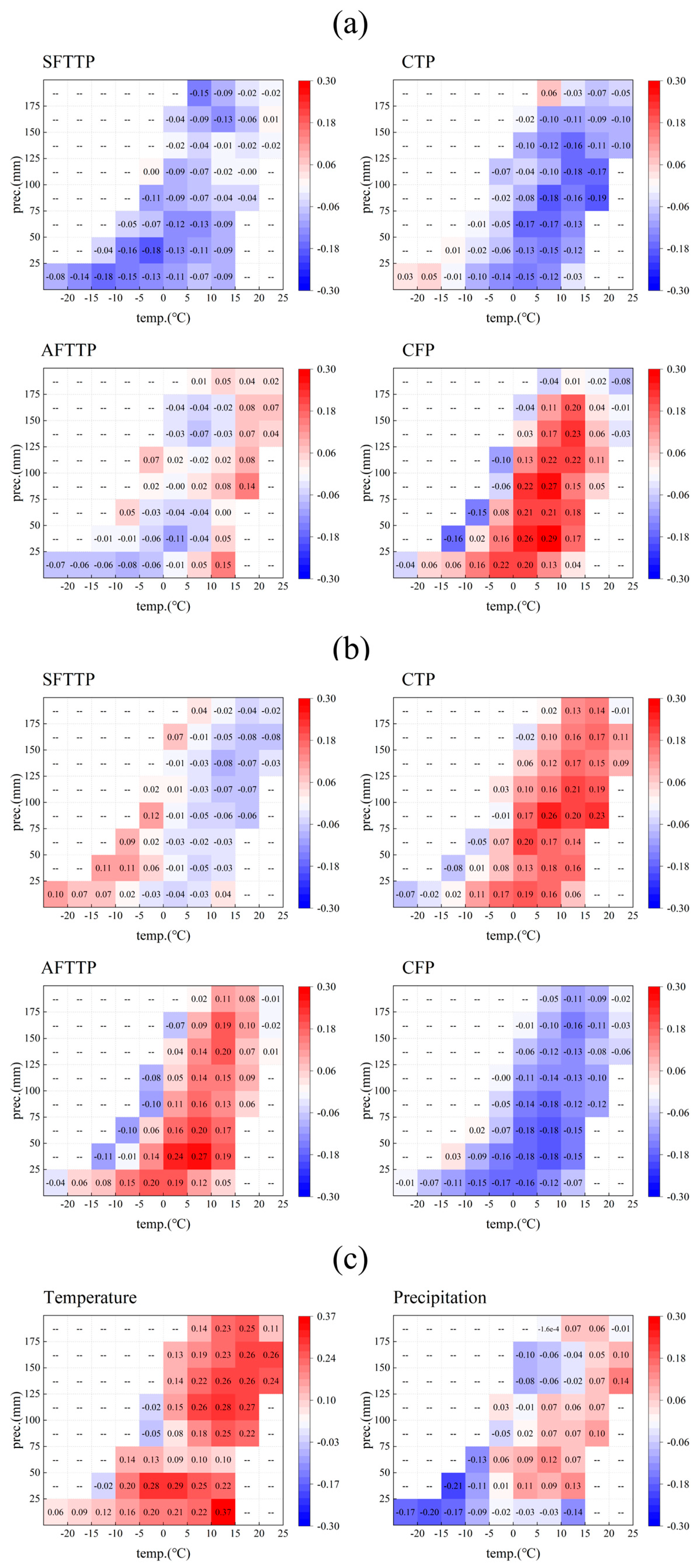
Temperature and the CTP are the main drivers of NDVI changes. The driving effect of the freeze–thaw transition period on NDVI showed obvious temporal and spatial differences: the onset date of the SFTTP has a stronger driving force on NDVI than its duration, while the AFTTP is the opposite. Precipitation and the CFP have the weakest dominance over NDVI in the region. In terms of the regulation of temperature and precipitation, cold and dry areas are more susceptible to the positive effects of the SFTTP, the CTP, and the AFTTP, while hot and rainy areas are more susceptible to the positive effects of the CFP. Areas with moderate precipitation are the least susceptible to the disturbances of freeze–thaw.

References

1. Henry, H.A.L. Soil freeze–thaw cycle experiments: Trends, methodological weaknesses and suggested improvements. Soil Biol. Biochem. 2007, 39, 977–986. [Google Scholar] [CrossRef]
2. Schimel, J.P.; Clein, J.S. Microbial response to freeze-thaw cycles in tundra and taiga soils. Soil Biol. Biochem. 1996, 28, 1061–1066. [Google Scholar] [CrossRef]
3. Hänninen, H.; Tanino, K. Tree seasonality in a warming climate. Trends Plant Sci. 2011, 16, 412–416. [Google Scholar] [CrossRef]
4. Musa, A.; Ya, L.; Anzhi, W.; Cunyang, N. Characteristics of soil freeze–thaw cycles and their effects on water enrichment in the rhizosphere. Geoderma 2016, 264, 132–139. [Google Scholar] [CrossRef]
5. Man, Z.; Weng, B.; Yang, Y.; Gong, X.; Li, M.; Yu, Z. Effects of the Freezing–Thawing Cycle Mode on Alpine Vegetation in the Nagqu River Basin of the Qinghai–Tibet Plateau. Water 2019, 11, 2122. [Google Scholar] [CrossRef]
6. Yang, J.; Wu, G.; Jiao, J.; Dyck, M.; He, H. Freeze-thaw induced landslides on grasslands in cold regions. CATENA 2022, 219, 106650. [Google Scholar] [CrossRef]
7. Wang, K.; Zhang, L.; Qiu, Y.; Ji, L.; Tian, F.; Wang, C.; Wang, Z. Snow effects on alpine vegetation in the Qinghai-Tibetan Plateau. Int. J. Digit. Earth 2015, 8, 58–75. [Google Scholar] [CrossRef]
8. Revuelto, J.; Gómez, D.; Alonso-González, E.; Vidaller, I.; Rojas-Heredia, F.; Deschamps-Berger, C.; García-Jiménez, J.; Rodríguez-López, G.; Sobrino, J.; Montorio, R.; et al. Intermediate snowpack melt-out dates guarantee the highest seasonal grasslands greening in the Pyrenees. Sci. Rep. 2022, 12, 18328. [Google Scholar] [CrossRef]
9. Song, Y.; Zou, Y.; Wang, G.; Yu, X. Altered soil carbon and nitrogen cycles due to the freeze-thaw effect: A meta-analysis. Soil Biol. Biochem. 2017, 109, 35–49. [Google Scholar] [CrossRef]
10. Zhang, Z.; Wang, Y.; Ma, Z.; Lv, M. Response mechanism of soil structural heterogeneity in permafrost active layer to freeze–thaw action and vegetation degradation. CATENA 2023, 230, 107250. [Google Scholar] [CrossRef]
11. Oztas, T.; Fayetorbay, F. Effect of freezing and thawing processes on soil aggregate stability. CATENA 2003, 52, 1–8. [Google Scholar] [CrossRef]
12. Dong, C.; Gu, Y.; Jia, Y.; Wei, P.; Jin, J.; Deng, Y.; Yang, P.; Chen, S. Effects of freeze-thaw cycles on the size distribution and stability of soil aggregate in the permafrost regions of the Qinghai-Tibetan Plateau. Environ. Res. Commun. 2023, 5, 095008. [Google Scholar] [CrossRef]
13. Yu, F.L.; Zhi, Q.X. The harm of low temperature to plants and the cold resistance of plants. Anim. Husb. Feed Sci. 2009, 30, 190. [Google Scholar] [CrossRef]
14. Li, T.; Fu, B.; Lü, Y.; Du, C.; Zhao, Z.; Wang, F.; Gao, G.; Wu, X. Soil freeze–thaw cycles affect spring phenology by changing phenological sensitivity in the Northern Hemisphere. Sci. Total Environ. 2024, 914, 169963. [Google Scholar] [CrossRef] [PubMed]
15. Lin, Z.; Zuo, Z.; Xiao, D.; You, Q. Soil moisture associated with freeze–thaw process modulated growing-season temperature rise in the Tibetan Plateau. Clim. Dyn. 2023, 61, 3619–3631. [Google Scholar] [CrossRef]
16. Bo, L.; Li, Z.; Li, P.; Xu, G.; Xiao, L.; Ma, B. Soil Freeze-Thaw and Water Transport Characteristics Under Different Vegetation Types in Seasonal Freeze-Thaw Areas of the Loess Plateau. Front. Earth Sci. 2021, 9, 704901. [Google Scholar] [CrossRef]
17. Cogato, A.; Meggio, F.; Collins, C.; Marinello, F. Medium-Resolution Multispectral Data from Sentinel-2 to Assess the Damage and the Recovery Time of Late Frost on Vineyards. Remote Sens. 2020, 12, 1896. [Google Scholar] [CrossRef]
18. Deng, G.; Zhang, H.; Yang, L.; Zhao, J.; Guo, X.; Ying, H.; Rihan, W.; Guo, D. Estimating Frost during Growing Season and Its Impact on the Velocity of Vegetation Greenup and Withering in Northeast China. Remote Sens. 2020, 12, 1355. [Google Scholar] [CrossRef]
19. Wang, C.; Li, K.; Chen, Q.; Ren, J.; He, X.; Li, S. Revealing the freezing-thawing hysteretic mechanisms of soil–water system based on soil microstructure. Geoderma 2024, 449, 116986. [Google Scholar] [CrossRef]
20. Grable, A.R. Soil Aeration and Plant Growth. Adv. Agron. 1966, 18, 57–106. [Google Scholar] [CrossRef]
21. Du, Z.; Cai, Y.; Wang, X.; Yan, Y.; Lu, X.; Liu, S. Research progress on the effects of soil freeze-thaw on plant physiology and ecology. Chin. J. Eco-Agric. 2014, 22, 1–9. [Google Scholar] [CrossRef]
22. Zhang, T.; Barry, R.G.; Knowles, K.; Heginbottom, J.A.; Brown, J. Statistics and characteristics of permafrost and ground-ice distribution in the Northern Hemisphere. Polar Geogr. 1999, 23, 132–154. [Google Scholar] [CrossRef]
23. Tian, X.H.; Zhang, L.F.; Zhang, X.; Chen, Z.G.; Zhao, L.; Li, Q.; Tang, Y.H.; Gu, S. Evapotranspiration characteristics of degraded meadow and effects of freeze-thaw changes in the Three-River Source Region. Acta Ecol. Sin. 2020, 40, 5649–5662. [Google Scholar] [CrossRef]
24. Fu, C.; Hu, Z.; Yang, Y.; Deng, M.; Yu, H.; Lu, S.; Wu, D.; Fan, W. Responses of Soil Freeze–Thaw Processes to Climate on the Tibetan Plateau from 1980 to 2016. Remote Sens. 2022, 14, 5907. [Google Scholar] [CrossRef]
25. Jia, G.J.; Zhou, Y.B.; Dai, L.M.; Zhou, W.M. Effects of freeze-thaw on soil carbon and nitrogen mineralization in Changbai Mountain forest. J. Environ. Ecol. Sci. 2012, 21, 624–628. [Google Scholar] [CrossRef]
26. Wang, G.; Zhang, Z.; Zhang, K. Responses of soil aggregates to freeze-thaw cycles under simulated experiments in typical black soils of Northeast China. J. Soils Sediments 2025, 25, 1100–1114. [Google Scholar] [CrossRef]
27. Zhang, Y.; Fu, Y.; Xu, J.; Li, Y.; Zhao, Y.; Wei, S.; Liu, B.; Zhang, X.; Lei, H.; Shao, S. Impact of freeze–thaw cycling on the stability and turnover of black soil aggregates. Geoderma 2024, 449, 117004. [Google Scholar] [CrossRef]
28. Jin, W.P.; Fan, H.M.; Liu, B.; Jiang, Y.Z.; Jiang, Y.; Ma, R.M. Effects of freeze-thaw alternation on the stability of black soil aggregates. Chin. J. Appl. Ecol. 2019, 30, 4195–4201. [Google Scholar] [CrossRef]
29. Chen, L.F.; He, Z.B.; Ming, J.; Du, J.; Lin, P.F.; Zhu, X. Review of the effects of freeze-thaw processes on soil respiration. Arid Zone Res. 2020, 37, 917–924. [Google Scholar]
30. Han, C.-L.; Gu, Y.-J.; Kong, M.; Hu, L.-W.; Jia, Y.; Li, F.-M.; Sun, G.-J.; Siddique, K.H.M. Responses of soil microorganisms, carbon and nitrogen to freeze–thaw cycles in diverse land-use types. Appl. Soil Ecol. 2018, 124, 211–217. [Google Scholar] [CrossRef]
31. Schimel, J.P.; Mikan, C. Changing microbial substrate use in Arctic tundra soils through a freeze-thaw cycle. Soil Biol. Biochem. 2005, 37, 1411–1418. [Google Scholar] [CrossRef]
32. Urakawa, R.; Shibata, H.; Kuroiwa, M.; Inagaki, Y.; Tateno, R.; Hishi, T.; Fukuzawa, K.; Hirai, K.; Toda, H.; Oyanagi, N.; et al. Effects of freeze–thaw cycles resulting from winter climate change on soil nitrogen cycling in ten temperate forest ecosystems throughout the Japanese archipelago. Soil Biol. Biochem. 2014, 74, 82–94. [Google Scholar] [CrossRef]
33. Kreyling, J.; Beierkuhnlein, C.; Jentsch, A. Effects of soil freeze–thaw cycles differ between experimental plant communities. Basic Appl. Ecol. 2010, 11, 65–75. [Google Scholar] [CrossRef]
34. Ren, J.Q.; Wang, D.N.; Liu, Y.X.; Li, J.P.; Guo, C.M.; Li, Q. Daily changes in soil freeze-thaw and their relationship with air and ground temperatures in Jilin Province. J. Glaciol. Geocryol. 2019, 41, 10. [Google Scholar]
35. Wu, Y.; Ouyang, W.; Hao, Z.; Lin, C.; Liu, H.; Wang, Y. Assessment of soil erosion characteristics in response to temperature and precipitation in a freeze-thaw watershed. Geoderma 2018, 328, 56–65. [Google Scholar] [CrossRef]
36. Dong, Q.X.; Luo, S.Q.; Wen, X.H.; Wang, J.Y.; Li, W.J. Changes in precipitation over the past 60 years in Southeast Tibet and their impact on soil temperature and freeze-thaw processes. Plateau Meteorol. 2022, 41, 404–419. [Google Scholar] [CrossRef]
37. Li, X.; Jin, R.; Pan, X.; Zhang, T.; Guo, J. Changes in the near-surface soil freeze–thaw cycle on the Qinghai-Tibetan Plateau. Int. J. Appl. Earth Obs. Geoinf. 2012, 17, 33–42. [Google Scholar] [CrossRef]
38. Yang, S.H.; Wu, T.H.; Li, R.; Zhu, X.F.; Wang, W.H.; Yu, W.J.; Qian, Y.H.; Hao, J.M. Spatial-temporal changes of the near-surface soil freeze-thaw status over the Qinghai-Tibetan Plateau. Plateau Meteorol. 2018, 37, 43–53. [Google Scholar] [CrossRef]
39. Xue, H.Z.; Jin, L.; Dong, G.T.; Zhang, H.J.; Li, Z.C. Characteristics of surface soil freeze-thaw status changes in the Hexi Corridor over the past 40 years. J. Soil Water Conserv. 2023, 37, 65–73+82. [Google Scholar] [CrossRef]
40. Song, C.; Dai, C.; Wang, C.; Yu, M.; Gao, Y.; Tu, W. Characteristic Analysis of the Spatio-Temporal Distribution of Key Variables of the Soil Freeze–Thaw Processes over Heilongjiang Province, China. Water 2022, 14, 2573. [Google Scholar] [CrossRef]
41. Liu, W.H.; Wen, J.; Chen, J.L.; Wang, Z.L.; Lu, X.C.; Wu, Y.Y.; Jiang, Y.Q. Analysis of the spatial and temporal distribution characteristics of key parameters in the soil freeze-thaw process on the Tibetan Plateau. Plateau Meteorol. 2022, 41, 11–23. [Google Scholar]
42. Liu, J.H.; Cui, J.F.; Guo, X.J.; Tang, X.Y. Bibliometric analysis of the impact of plant roots on soil water movement. Chin. J. Soil Sci. 2024, 55, 1163–1173. [Google Scholar] [CrossRef]
43. Lai, X.; Yao, S.; Cen, S.; Zhang, G.; Zhang, Z.; Zhang, S. Changes in the spatiotemporal distribution of the timing and duration of the soil freeze–thaw status from 1979 to 2018 over the Tibetan Plateau. Int. J. Climatol. 2024, 44, 4963–4983. [Google Scholar] [CrossRef]
44. Shi, F.X.; Qin, J.; Han, T.D.; Cui, J.H.; Ding, Y.J.; Cheng, P.; You, Y.H. Changes in seasonal frozen soil freeze-thaw characteristic parameters and their influencing factors in cold mountainous areas: A case study of the southern slope of the Tianshan Mountains. J. Glaciol. Geocryol. 2024, 46, 89–100. [Google Scholar]
45. Ravindra, K.; Rattan, P.; Mor, S.; Aggarwal, A.N. Generalized additive models: Building evidence of air pollution, climate change and human health. Environ. Int. 2019, 132, 104987. [Google Scholar] [CrossRef] [PubMed]
46. Brunsdon, C.; Fotheringham, A.S.; Charlton, M.E. Geographically weighted regression: A method for exploring spatial nonstationarity. Geogr. Anal. 1996, 28, 281–298. [Google Scholar] [CrossRef]
47. Torrence, C.; Compo, G.P. A practical guide to wavelet analysis. Bull. Am. Meteorol. Soc. 1998, 79, 61–78. [Google Scholar] [CrossRef]
48. Meng, B.; Liang, T.; Yi, S.; Yin, J.; Cui, X.; Ge, J.; Hou, M.; Lv, Y.; Sun, Y. Modeling Alpine Grassland Above Ground Biomass Based on Remote Sensing Data and Machine Learning Algorithm: A Case Study in East of the Tibetan Plateau, China. IEEE J. Sel. Top. Appl. Earth Obs. Remote Sens. 2020, 13, 2986–2995. [Google Scholar] [CrossRef]
49. Zhou, D.; Tang, M.; Li, H. Investigating the nonlinear effects of climate change on agricultural green total factor productivity: Findings from the PSTR approach. Environ. Dev. Sustain. 2024, 26, 24453–24471. [Google Scholar] [CrossRef]
50. Wang, J.; Wu, Q.; Yuan, Z.; Kang, H. Soil respiration of alpine meadow is controlled by freeze–thaw processes of active layer in the permafrost region of the Qinghai–Tibet Plateau. Cryosphere 2020, 14, 2835–2848. [Google Scholar] [CrossRef]
51. Boli, C.; Siqiong, L.; Shihua, L.; Yu, Z.; Di, M. Effects of the soil freeze-thaw process on the regional climate of the Qinghai-Tibet Plateau. Clim. Res. 2014, 59, 243–257. [Google Scholar] [CrossRef]
52. Feng, Y.Q.; Liang, S.H.; Wu, Q.B.; Chen, J.W.; Tian, X.; Wu, P. Changes in vegetation cover during permafrost degradation. J. Beijing Norm. Univ. (Nat. Sci.) 2016, 52, 311–316. [Google Scholar] [CrossRef]
53. Yang, Y.; Wang, X.; Wang, T. Permafrost Degradation Induces the Abrupt Changes of Vegetation NDVI in the Northern Hemisphere. Earth’s Future 2024, 12, e2023EF004309. [Google Scholar] [CrossRef]
54. Cheng, Z.; Wang, F.; Sun, J.; Ding, L.; Wang, Y.; Wang, H. Effect of seasonal freeze–thaw process on spatial and temporal distribution of soil water and its infiltration to recharge groundwater. Hydrol. Process. 2024, 38, e15110. [Google Scholar] [CrossRef]
55. He, Y.Y.; Peng, Q.L.; Wang, L.; Wang, S.M.; Er, L.; Xu, Y.; Lv, Y.; Chen, Y.; Zhang, X.W. Pore characteristics and permeability of peat soil in seasonal frozen zones: A study based on multiple microscopic methods. Rock Soil Mech. 2025, 46, 110–122. [Google Scholar] [CrossRef]
56. Zheng, X.Y.; Chen, P.; Han, J.J.; Meng, Z.X.; Wang, Y.N.; Lin, J.X.; Wang, J.H. Advances in the effects of freeze-thaw cycles on soil aggregates and microbial properties. J. Jiangsu Agric. Sci. 2023, 39, 1080–1088. [Google Scholar] [CrossRef]
57. Du, Z.Y. Effects of freeze-thaw cycles on the physical, chemical, and biological properties of alpine meadow soils. J. Environ. Ecol. Sci. 2020, 29, 1054–1061. [Google Scholar] [CrossRef]
58. Feng, X.; Nielsen, L.L.; Simpson, M.J. Responses of soil organic matter and microorganisms to freeze–thaw cycles. Soil Biol. Biochem. 2007, 39, 2027–2037. [Google Scholar] [CrossRef]
59. Shi, G.; Hou, R.; Li, T.; Fu, Q.; Wang, J.; Zhou, W.; Su, Z.; Shen, W.; Wang, Y. Effects of biochar and freeze–thaw cycles on the bacterial community and multifunctionality in a cold black soil area. J. Environ. Manag. 2023, 342, 118302. [Google Scholar] [CrossRef] [PubMed]
60. Luo, S.; Wang, J.; Pomeroy, J.W.; Lyu, S. Freeze–Thaw Changes of Seasonally Frozen Ground on the Tibetan Plateau from 1960 to 2014. J. Clim. 2020, 33, 9427–9446. [Google Scholar] [CrossRef]
61. Peng, X.; Frauenfeld, O.W.; Cao, B.; Wang, K.; Wang, H.; Su, H.; Huang, Z.; Yue, D.; Zhang, T. Response of changes in seasonal soil freeze/thaw state to climate change from 1950 to 2010 across China. J. Geophys. Res. Earth Surf. 2016, 121, 1984–2000. [Google Scholar] [CrossRef]
62. Zhao, L.; Zou, D.; Hu, G.; Du, E.; Pang, Q.; Xiao, Y.; Li, R.; Sheng, Y.; Wu, X.; Sun, Z.; et al. Changing climate and the permafrost environment on the Qinghai–Tibet (Xizang) plateau. Permafr. Periglac. Process. 2020, 31, 396–405. [Google Scholar] [CrossRef]
63. Wang, M.; Zhou, C.P.; Wu, L.; Xu, X.L.; Ouyang, H. A study on the dry and wet conditions of the Tibetan Plateau over the past 10 years and their relationship with vegetation changes. J. Arid Land Geogr. 2013, 36, 49–56. Available online: https://www.webofscience.com/wos/alldb/full-record/CSCD:4781398 (accessed on 25 April 2025).
64. Wu, Y.; Li, F.; Zhang, J.; Liu, Y.; Li, H.; Zhou, B.; Shen, B.; Hou, L.; Xu, D.; Ding, L.; et al. Spatial and temporal patterns of above- and below- ground biomass over the Tibet Plateau grasslands and their sensitivity to climate change. Sci. Total Environ. 2024, 919, 170900. [Google Scholar] [CrossRef]
65. Xu, R.; Wang, Z.; Zhu, J. Effects of Climate Change and Nitrogen Addition on Carbon Loss in Alpine Wetland of Qinghai–Tibet Plateau. Atmosphere 2023, 14, 1342. [Google Scholar] [CrossRef]
66. Chen, B.; Zhang, X.; Tao, J.; Wu, J.; Wang, J.; Shi, P.; Zhang, Y.; Yu, C. The impact of climate change and anthropogenic activities on alpine grassland over the Qinghai-Tibet Plateau. Agric. For. Meteorol. 2014, 189–190, 11–18. [Google Scholar] [CrossRef]
67. Song, C.; Wang, G.; Sun, X.; Hu, Z. River runoff components change variably and respond differently to climate change in the Eurasian Arctic and Qinghai-Tibet Plateau permafrost regions. J. Hydrol. 2021, 601, 126653. [Google Scholar] [CrossRef]
68. Shan, S.; Shen, R.; Shi, C.; Bai, L.; Sun, S. Evaluation of land surface temperature and 2 m air temperature from five reanalyses datasets across North China in Winter. Plateau Meteorol. 2020, 39, 37–47. [Google Scholar]
69. Apaydin, H.; Kemal Sonmez, F.; Yildirim, Y.E. Spatial interpolation techniques for climate data in the GAP region in Turkey. Clim. Res. 2004, 28, 31–40. [Google Scholar] [CrossRef]
70. Keys, R. Cubic convolution interpolation for digital image processing. IEEE Trans. Acoust. Speech Signal Process. 1981, 29, 1153–1160. [Google Scholar] [CrossRef]
71. Yang, M.; Yao, T.; Gou, X.; Hirose, N.; Fujii, H.Y.; Hao, L.; Levia, D.F. Diurnal freeze/thaw cycles of the ground surface on the Tibetan Plateau. Chin. Sci. Bull. 2006, 51, 1974–1976. [Google Scholar] [CrossRef]
72. Yue, S.P.; Yan, Y.C.; Zhang, S.W.; Yang, J.C.; Wang, W.J. Spatiotemporal variations of soil freeze-thaw state in Northeast China based on the ERA5-LAND dataset. Acta Geogr. Sin. 2021, 76, 2765–2779. [Google Scholar] [CrossRef]
73. Yue, S.; Pilon, P.; Cavadias, G. Power of the Mann–Kendall and Spearman’s rho tests for detecting monotonic trends in hydrological series. J. Hydrol. 2002, 259, 254–271. [Google Scholar] [CrossRef]
74. Li, H.; Cao, Y.; Xiao, J.; Yuan, Z.; Hao, Z.; Bai, X.; Wu, Y.; Liu, Y. A daily gap-free normalized difference vegetation index dataset from 1981 to 2023 in China. Sci. Data 2024, 11, 527. [Google Scholar] [CrossRef]
75. Wang, Y.; Wang, X.; Li, C.; Wu, F.; Yang, Z. Spatiotemporal analysis of temperature trends under climate change in the source region of the Yellow River, China. Theor. Appl. Clim. 2015, 119, 123–133. [Google Scholar] [CrossRef]
76. Yang, X.; Xie, X.; Liu, D.L.; Ji, F.; Wang, L. Spatial interpolation of daily rainfall data for local climate impact assessment over greater sydney region. Adv. Meteorol. 2015, 2015, 563629. [Google Scholar] [CrossRef]
77. Qi, H.Q.; Chen, M. The non-linear characteristics of the impact of environmental regulation on China’s green economic efficiency. J. Quant. Econ. 2018, 9, 61–77. [Google Scholar] [CrossRef]
78. Gong, F.; Wang, Z.; Yu, J.L. Population aging, intergenerational balance, and public welfare expenditure. Econ. Res. J. 2019, 54, 103–119. [Google Scholar]
79. Qi, H.Q.; Yan, H.C. Does population aging inhibit China’s economic growth? Econ. Rev. 2018, 6, 28–40. [Google Scholar] [CrossRef]
80. Gonzalez, A.; Terasvirta, T.; Dijk, D.V. Panel Smooth Transition Regression Models; Research Paper; Stockholm School of Economics: Stockholm, Sweden, 2005. [Google Scholar]
81. Colletaz, G.; Hurlin, C. Threshold Effects of the Public Capital Productivity: An International Panel Smooth Transition Approach. Leo Working Papers/DR LEO. 2006. Available online: https://shs.hal.science/halshs-00008056 (accessed on 25 April 2025).
82. Fouquau, J.; Hurlin, C.; Rabaud, I. The Feldstein-Horioka Puzzle: A Panel Smooth Transition Regression Approach. Econ. Model. 2007, 2, 284–299. [Google Scholar]
83. Zhao, Y.; Chen, Y.; Wu, C.; Li, G.; Ma, M.; Fan, L.; Zheng, H.; Song, L.; Tang, X. Exploring the contribution of environmental factors to evapotranspiration dynamics in the Three-River-Source region, China. J. Hydrol. 2023, 626, 130222. [Google Scholar] [CrossRef]
84. Wang, T.; Yang, D.; Zheng, G.; Shi, R. Possible negative effects of earlier thaw onset and longer thaw duration on vegetation greenness over the Tibetan Plateau. Agric. For. Meteorol. 2022, 326, 109192. [Google Scholar] [CrossRef]
85. Wang, Z.; Sha, Z.J.; Ma, Y.J.; Hu, J.F.; Zhai, Y.L.; Ma, H.Y. Spatial distribution characteristics and intensity of soil freeze-thaw erosion in alpine meadow regions based on GIS. J. Earth Environ. 2017, 8, 55–64. [Google Scholar]
86. Yang, L.; Cui, G.S.; Xia, C.X.; Lamu, A.; Sun, J.; Wang, J.N.; Luo, D.L.; Zhang, L. The ecological responses and adaptability of alpine shrubs to global warming. Pratacultural Sci. 2023, 40, 378–393. [Google Scholar] [CrossRef]
87. Zhang, L.; Ren, F.; Li, H.; Cheng, D.; Sun, B. The Influence Mechanism of Freeze-Thaw on Soil Erosion: A Review. Water 2021, 13, 1010. [Google Scholar] [CrossRef]
88. Zhou, W.; Chen, H.; Zhou, L.; Lewis, B.J.; Ye, Y.; Tian, J.; Li, G.; Dai, L. Effect of freezing-thawing on nitrogen mineralization in vegetation soils of four landscape zones of Changbai Mountain. Ann. For. Sci. 2011, 68, 943–951. [Google Scholar] [CrossRef]
89. Xu, L.; Myneni, R.B.; Chapin, F.S., III; Callaghan, T.V.; Pinzon, J.E.; Tucker, C.J.; Zhu, Z.; Bi, J.; Ciais, P.; Tømmervik, H.; et al. Temperature and vegetation seasonality diminishment over northern lands. Nat. Clim. Change 2013, 3, 581–586. [Google Scholar] [CrossRef]
90. Wipf, S.; Rixen, C. A review of snow manipulation experiments in Arctic and alpine tundra ecosystems. Polar Res. 2010, 29, 95–109. [Google Scholar] [CrossRef]
91. Richardson, A.D.; Hufkens, K.; Milliman, T.; Aubrecht, D.M.; Furze, M.E.; Seyednasrollah, B.; Krassovski, M.B.; Latimer, J.M.; Nettles, W.R.; Heiderman, R.R.; et al. Ecosystem warming extends vegetation activity but heightens vulnerability to cold temperatures. Nature 2018, 560, 368–371. [Google Scholar] [CrossRef]
92. Hu, J.; Moore, D.J.P.; Burns, S.P.; Monson, R.K. Longer growing seasons lead to less carbon sequestration by a subalpine forest. Glob. Change Biol. 2010, 16, 771–783. [Google Scholar] [CrossRef]
93. Zhang, G.; Liu, X.; Wang, J.; Liu, J.; Zhao, X.; Li, H.; Wang, R.; Luo, X.; Xing, L.; Wang, C.; et al. Spatial and temporal distribution and environmental determinants of freeze-thaw erosion intensity in Qiangtang grasslands, China. Soil Res. 2024, 62, SR23216. [Google Scholar] [CrossRef]
94. Sun, B.Y.; Li, Z.B.; Xiao, J.B.; Zhang, L.T.; Ma, B.; Li, J.M.; Cheng, D.B. Advances in the effects of freeze-thaw cycles on soil physical and chemical properties and wind-water erosion. Chin. J. Appl. Ecol. 2019, 30, 337–347. [Google Scholar] [CrossRef]
95. Li, N.; Cuo, L.; Zhang, Y. On the freeze–thaw cycles of shallow soil and connections with environmental factors over the Tibetan Plateau. Clim. Dyn. 2021, 57, 3183–3206. [Google Scholar] [CrossRef]
96. Wang, G.; Hu, H.; Li, T. The influence of freeze–thaw cycles of active soil layer on surface runoff in a permafrost watershed. J. Hydrol. 2009, 375, 438–449. [Google Scholar] [CrossRef]
97. Zheng, D.; van der Velde, R.; Su, Z.; Wen, J.; Wang, X.; Yang, K. Impact of soil freeze-thaw mechanism on the runoff dynamics of two Tibetan rivers. J. Hydrol. 2018, 563, 382–394. [Google Scholar] [CrossRef]
98. Jing, G.C.; Ren, X.P.; Liu, X.J.; Liu, B.Y.; Zhang, L.H.; Yang, Y.J.; Wang, Y.J. Relationship between freeze-thaw cycles and soil moisture in the Northeast Black Soil Region. Chin. J. Soil Water Conserv. 2008, 2008, 32–36. [Google Scholar] [CrossRef]
99. Wang, L.; Liao, D.; Rengel, Z.; Shen, J. Soil–plant–microbe interactions in the rhizosphere: Incremental amplification induced by localized fertilization. Front. Agric. Sci. Eng. 2025, 12, 57–68. [Google Scholar] [CrossRef]
100. Yang, K.; Wang, C. Water storage effect of soil freeze-thaw process and its impacts on soil hydro-thermal regime variations. Agric. For. Meteorol. 2019, 265, 280–294. [Google Scholar] [CrossRef]
101. Yu, X.; Zou, Y.; Jiang, M.; Lu, X.; Wang, G. Response of soil constituents to freeze–thaw cycles in wetland soil solution. Soil Biol. Biochem. 2011, 43, 1308–1320. [Google Scholar] [CrossRef]
102. Groffman, P.M.; Driscoll, C.T.; Fahey, T.J.; Hardy, J.P.; Fitzhugh, R.D.; Tierney, G.L. Effects of mild winter freezing on soil nitrogen and carbon dynamics in a northern hardwood forest. Biogeochemistry 2001, 56, 191–213. [Google Scholar] [CrossRef]
103. Brooks, P.D.; Williams, M.W.; Schmidt, S.K. Inorganic nitrogen and microbial biomass dynamics before and during spring snowmelt. Biogeochemistry 1998, 43, 1–15. [Google Scholar] [CrossRef]
104. Richardson, A.D.; Keenan, T.F.; Migliavacca, M.; Ryu, Y.; Sonnentag, O.; Toomey, M. Climate change, phenology, and phenological control of vegetation feedbacks to the climate system. Agric. For. Meteorol. 2013, 169, 156–173. [Google Scholar] [CrossRef]
105. Euskirchen, E.S.; McGuire, A.D.; Kicklighter, D.W.; Zhuang, Q.; Lein, J.S.C.; Dargaville, R.J.; Dye, D.G.; Kimball, J.S.; McDonald, K.C.; Melillo, J.M.; et al. Importance of recent shifts in soil thermal dynamics on growing season length, productivity, and carbon sequestration in terrestrial high-latitude ecosystems. Glob. Change Biol. 2006, 12, 731–750. [Google Scholar] [CrossRef]
106. Yu, Z.J.; Yang, P. Climate change in the Beijing-Tianjin-Hebei region over the past 50 years and its impact on soil moisture. Guizhou Agric. Sci. 2019, 47, 144–149. [Google Scholar] [CrossRef]
107. Zhu, C.J.; Gao, J.X. A review of factors influencing soil evaporation and its suppression methods. Environ. Prot. Sci. 2024, 50, 19–26. [Google Scholar] [CrossRef]
108. Sun, M.X.; Zhang, Y.; Xin, Y.; Zhong, D.J.; Yang, C.J. Vegetation phenology changes and their responses to climate change on the Western Sichuan Plateau over the past 20 years. Ecol. Environ. Sci. 2022, 31, 1326–1339. [Google Scholar] [CrossRef]
109. Misra, D.; Dutta, W.; Jha, G.; Ray, P. Interactions and Regulatory Functions of Phenolics in Soil-Plant-Climate Nexus. Agronomy 2023, 13, 280. [Google Scholar] [CrossRef]
110. Chen, Z.; Zhang, X.; Huang, Y.; Shi, Z.; Yao, H. Mechanisms of plant phenolic compounds affecting soil nitrogen transformation. Alex. Eng. J. 2025, 120, 173–184. [Google Scholar] [CrossRef]
111. Zhang, J.; Hao, F.H.; Wu, Z.F.; Li, M.W.; Zhang, X.; Fu, Y.S. Response of vegetation phenology to extreme climate and its mechanism. Acta Geogr. Sin. 2023, 78, 2241–2255. [Google Scholar] [CrossRef]
112. Pang, B.; Hong, J.; Ma, X.; Qin, X.; Wang, X. Nitrogen absorption strategy of Stipa purpurea, a typical species in alpine grassland during freeze-thaw cycle. Acta Ecol. Sin. 2023, 43, 1147–1155. [Google Scholar] [CrossRef]
113. Lin, S.; Li, H.Y.; Huang, P.C.; Duan, X.Y. Characteristics of high temperature, drought and circulation situation in summer 2022 in China. J. Arid Meteorol. 2022, 40, 748–763. [Google Scholar]
114. Liu, D.; He, Y.H.; Zhang, L.L.; Li, J.M. Effects of freeze-thaw cycles on soil structure under different conditions. J. Northeast Agric. Univ. 2023, 54, 58–72. [Google Scholar] [CrossRef]
115. Liu, F.; Zhang, W.; Li, S. Effects of Freeze–Thaw Cycles on Uptake Preferences of Plants for Nutrient: A Review. Plants 2025, 14, 1122. [Google Scholar] [CrossRef] [PubMed]
116. Körner, C. Plant Ecology at High Elevations. In Alpine Plant Life; Springer International Publishing: Berlin/Heidelberg, Germany, 2021; pp. 1–22. [Google Scholar] [CrossRef]
117. Zhang, K.-L.; Leng, Y.-N.; Hao, R.-R.; Zhang, W.-Y.; Li, H.-F.; Chen, M.-X.; Zhu, F.-Y. Adaptation of High-Altitude Plants to Harsh Environments: Application of Phenotypic-Variation-Related Methods and Multi-Omics Techniques. Int. J. Mol. Sci. 2024, 25, 12666. [Google Scholar] [CrossRef] [PubMed]
118. Liu, X.J.; Chen, R.S.; Liu, J.F.; Wang, X.Q.; Zhang, B.G.; Liu, G.H. Variation of snow cover and its influence on spring runoff in the source region of the Yellow River. Plateau Meteorol. 2020, 39, 226–233. [Google Scholar] [CrossRef]
119. Rixen, C.; Høye, T.T.; Macek, P.; Aerts, R.; Alatalo, J.M.; Anderson, J.T.; Arnold, P.A.; Barrio, I.C.; Bjerke, J.W.; Björkman, M.P.; et al. Winters are changing: Snow effects on Arctic and alpine tundra ecosystems. Arct. Sci. 2022, 8, 572–608. [Google Scholar] [CrossRef]
120. Wang, F.; Lai, H.; Li, Y.; Feng, K.; Zhang, Z.; Tian, Q.; Zhu, X.; Yang, H. Dynamic variation of meteorological drought and its relationships with agricultural drought across China. Agric. Water Manag. 2022, 261, 107301. [Google Scholar] [CrossRef]
121. Huang, J.; Yu, H.; Guan, X.; Wang, G.; Guo, R. Accelerated dryland expansion under climate change. Nat. Clim. Change 2016, 6, 166–171. [Google Scholar] [CrossRef]
122. Jin, K.; Wang, F.; Han, J.Q.; Shi, S.Y.; Ding, W.B. Contribution of climatic change and human activities to vegetation NDVI change over China during 1982–2015. Acta Geogr. Sin. 2020, 75, 961–974. [Google Scholar] [CrossRef]
123. Chen, J.H.; Lu, Q.; Liu, Y.Q.; He, C.Y.; Yan, F. Distribution and influencing factors of freeze-thaw desertification degradation areas on the Tibetan Plateau. Res. Soil Water Conserv. 2023, 30, 103–110+120. [Google Scholar] [CrossRef]
124. Geng, Q.L.; Chen, X.Q.; He, X.H.; Tian, Z.H. Vegetation dynamics and its response to climate change and human activities based on different vegetation types in China. Acta Ecol. Sin. 2022, 38, 63–72. [Google Scholar] [CrossRef]
125. Yang, T.; Cong, N. Response of spring vegetation phenology to soil freeze–thaw state in the Northern Hemisphere from 2016 to 2022. Front. For. Glob. Change 2023, 6, 1332734. [Google Scholar] [CrossRef]
126. Jia, D.; Liu, M.; Li, K.; Wang, X.; Wang, Z.; Wen, J.; Lai, X. Variations in the top-layer soil freezing/thawing process from 2009 to 2018 in the Maqu area of the Tibetan Plateau. Theor. Appl. Climatol. 2021, 143, 21–32. [Google Scholar] [CrossRef]
127. Shao, W.W.; Zhang, T.J. Comparison and analysis of the near-surface soil freeze/thaw status datasets obtained by passive microwave remote sensing. J. Glaciol. Geocryol. 2021, 43, 285–295. [Google Scholar] [CrossRef]
128. Qin, X.; Nie, X.; Wang, X.; Hong, J. Freeze-thaw process induced by increased precipitation affects root growth of alpine steppe on the Tibetan Plateau. J. Mt. Sci. 2023, 20, 3010–3017. [Google Scholar] [CrossRef]
129. Xu, H.; Wang, F.; Li, T.; Wu, X. A review of freezing-thawing cycle effects on key processes of soil nitrogen cycling and the underlying mechanisms. Acta Ecol. Sin. 2020, 40, 3168–3182. [Google Scholar] [CrossRef]
130. Dai, L.C.; Ke, X.; Zhang, F.W.; Du, Y.G.; Li, Y.K.; Guo, X.W.; Li, Q.; Lin, L.; Cao, G.M. Characteristics of hydro-thermal coupling during soil freezing-thawing process in seasonally frozen soil regions on the Tibetan Plateau. J. Glaciol. Geocryol. 2020, 42, 390–398. [Google Scholar] [CrossRef]
131. Zhang, Y.L.; Yin, B.F.; Tao, Y.; Zhou, X.B.; Zhang, Y.M. Effects of freeze-thaw processes on the germination of desert ephemeral plant seeds. Chin. J. Ecol. 2021, 40, 301–312. [Google Scholar] [CrossRef]
132. Zahedi, S.M.; Karimi, M.; Venditti, A.; Zahra, N.; Siddique, K.H.M.; Farooq, M. Plant Adaptation to Drought Stress: The Role of Anatomical and Morphological Characteristics in Maintaining the Water Status. J. Soil Sci. Plant Nutr. 2025, 25, 409–427. [Google Scholar] [CrossRef]
133. Maeght, J.-L.; Rewald, B.; Pierret, A. How to study deep roots—And why it matters. Front. Plant Sci. 2013, 4, 299. [Google Scholar] [CrossRef]
134. Borowik, A.; Wyszkowska, J. Impact of temperature on the biological properties of soil. Int. Agrophysics 2016, 30, 1–8. [Google Scholar] [CrossRef]
135. Knight, C.G.; Nicolitch, O.; Griffiths, R.I.; Goodall, T.; Jones, B.; Weser, C.; Langridge, H.; Davison, J.; Dellavalle, A.; Eisenhauer, N.; et al. Soil microbiomes show consistent and predictable responses to extreme events. Nature 2024, 636, 690–696. [Google Scholar] [CrossRef]
136. Fromin, N. Impacts of soil storage on microbial parameters. SOIL 2025, 11, 247–265. [Google Scholar] [CrossRef]
137. Hetherington, A.; Woodward, F. The role of stomata in sensing and driving environmental change. Nature 2003, 424, 901–908. [Google Scholar] [CrossRef]
138. Gampe, D.; Zscheischler, J.; Reichstein, M.; O’Sullivan, M.; Smith, W.K.; Sitch, S.; Buermann, W. Increasing impact of warm droughts on northern ecosystem productivity over recent decades. Nat. Clim. Change 2021, 11, 772–779. [Google Scholar] [CrossRef]
139. Walther, G.-R.; Post, E.; Convey, P.; Menzel, A.; Parmesan, C.; Beebee, T.J.C.; Fromentin, J.-M.; Hoegh-Guldberg, O.; Bairlein, F. Ecological responses to recent climate change. Nature 2002, 416, 389–395. [Google Scholar] [CrossRef]
140. Chen, J.Z.; Zhao, C.S.; Zhang, X.Z. Changes in vegetation growing season and active accumulated temperature in circum-Arctic region under 21st century climate change scenario. Clim. Environ. Res. 2020, 25, 543–554. [Google Scholar] [CrossRef]
141. Jiang, M.; Li, H.; Zhang, W.; Liu, J.; Zhang, Q. Effects of climate change and grazing on the soil organic carbon stock of alpine wetlands on the Tibetan Plateau from 2000 to 2018. CATENA 2024, 238, 107870. [Google Scholar] [CrossRef]
142. Li, Z.; Qu, H.; Li, L.; Zheng, J.; Wei, D.; Wang, F. Effects of climate change on vegetation dynamics of the Qinghai-Tibet Plateau, a causality analysis using empirical dynamic modeling. Heliyon 2023, 9, e16001. [Google Scholar] [CrossRef]
143. Xiang, H.T.; Zheng, D.F.; He, N.; Li, W.; Wang, M.L.; Wang, S.Y. Research progress on the physiological response of plants to low temperature and the amelioration effectiveness of exogenous ABA. Acta Prataculturae Sin. 2021, 30, 208–219. [Google Scholar]
144. Li, Z.H.; Li, J.Y.; Wang, F.; Xin, Y.L. Advances in the response mechanisms of plants to low-temperature stress. Agric. Technol. 2024, 44, 134–138. [Google Scholar] [CrossRef]
145. Sun, S.K.; Liu, X.K.; Zhu, X.Y.; Duan, X.H.; Han, H.F. Advances in the migration and leaching of soil dissolved organic carbon and nitrogen. Shanxi Agric. Sci. 2022, 50, 1158–1167. [Google Scholar]
146. Li, M.H.; Du, J.K.; Li, W.T.; Li, R.J.; Wang, S.Y.; Wang, S.S. Global vegetation changes and their relationships with temperature and precipitation from 1982 to 2015. J. Geogr. Sci. 2020, 40, 823–832. [Google Scholar] [CrossRef]
147. Li, S.C.; Li, D.L.; Zhao, P.; Zhang, G.Q. The climatic characteristics of vapor transportation in rainy season of the origin area of three rivers in Qinghai-Xizang Plateau. Acta Meteorol. Sin. 2009, 4, 591–598. [Google Scholar] [CrossRef]
148. He, W.; Bu, R.C.; Xiong, Z.P.; Hu, Y.M. Characteristics of temperature and precipitation in Northeastern China from 1961 to 2005. Acta Ecol. Sin. 2013, 33, 519–531. [Google Scholar] [CrossRef]
149. Wang, N. Simulation Research on Snow Melting Process in Spring. Open J. Nat. Sci. 2022, 10, 138–145. [Google Scholar] [CrossRef]
150. Zhang, W.; Shen, Y.; Wang, X.; Kang, S.; Chen, A.; Mao, W.; Zhong, X. Snow cover controls seasonally frozen ground regime on the southern edge of Altai Mountains. Agric. For. Meteorol. 2021, 297, 108271. [Google Scholar] [CrossRef]
151. Feng, X.L.; Li, H.M.; Luo, S.Q.; Bai, W.R.; Wen, T.T. Freeze-Thaw Characteristics of Seasonally Frozen Ground in the Three River Source Region from 1961 to 2020. Plateau Meteorol. 2022, 41, 295–305. [Google Scholar] [CrossRef]
152. Shen, Q.K.; Liu, X.G.; Zhou, X.; Zhang, Z.J.; Chen, Q.H. Spatio-temporal variation patterns of diurnal freeze-thaw cycles of the near-surface soil on the Qinghai-Tibet Plateau between 2002 and 2020. Acta Geogr. Sin. 2023, 78, 587–603. [Google Scholar] [CrossRef]
153. Zhu, Y.; Fan, G.Z.; Hua, W.; Wang, Q.R. Spatiotemporal variation characteristics of surface temperature on the Tibetan Plateau from 1981 to 2015. J. Southwest Univ. (Nat. Sci. Ed.) 2018, 40, 127–140. [Google Scholar] [CrossRef]
154. Wei, Y.; Li, X.; Gu, L.; Zheng, Z.; Zheng, X.; Jiang, T. Significant decreasing trends in snow cover and duration in Northeast China during the past 40 years from 1980 to 2020. J. Hydrol. 2023, 626, 130318. [Google Scholar] [CrossRef]
155. Tong, Y.; Sorokin, A. What Are Black Soils and Why Are Black Soils Important in Multiregional Aspects? Mosc. Univ. Soil Sci. Bull. 2024, 79, 603–607. [Google Scholar] [CrossRef]
156. Gu, Z.K.; Du, G.Z.; Zhu, W.X.; Suo, N.J.; Zhang, S.H. Distribution patterns of soil nutrients in different grassland types in eastern Tibetan Plateau. Pratacultural Sci. 2012, 29, 507–512. [Google Scholar]
157. Pei, L.-L.; Feng, J.-L.; Zhang, W.; Lin, Y.-C.; Hu, H.-P.; Wang, K.-Y.; Chen, Y.-Y.; Zhang, Q. Anomalous water retention capacity of alpine meadow soil with eolian dust accretion on the Tibetan Plateau. CATENA 2022, 213, 106159. [Google Scholar] [CrossRef]
158. Hu, G.; Zhao, L.; Li, R.; Wu, X.; Wu, T.; Xie, C.; Zhu, X.; Su, Y. Variations in soil temperature from 1980 to 2015 in permafrost regions on the Qinghai-Tibetan Plateau based on observed and reanalysis products. Geoderma 2019, 337, 893–905. [Google Scholar] [CrossRef]
159. Chang, X.; Jin, H.; Zhang, Y.; He, R.; Luo, D.; Wang, Y.; Lü, L.; Zhang, Q. Thermal Impacts of Boreal Forest Vegetation on Active Layer and Permafrost Soils in Northern da Xing’Anling (Hinggan) Mountains, Northeast China. Arct. Antarct. Alp. Res. 2015, 47, 267–279. [Google Scholar] [CrossRef]
160. Zhang, J.; Sun, J.; Ma, B.; Du, W. Assessing the ecological vulnerability of the upper reaches of the Minjiang River. PLoS ONE 2017, 12, e0181825. [Google Scholar] [CrossRef]
161. Xia, M.; Jia, K.; Zhao, W.; Liu, S.; Wei, X.; Wang, B. Spatio-temporal changes of ecological vulnerability across the Qinghai-Tibetan Plateau. Ecol. Indic. 2021, 123, 107274. [Google Scholar] [CrossRef]
162. Xu, Y.; Dong, S.; Shen, H.; Xiao, J.; Li, S.; Gao, X.; Wu, S. Degradation significantly decreased the ecosystem multifunctionality of three alpine grasslands: Evidences from a large-scale survey on the Qinghai-Tibetan Plateau. J. Mt. Sci. 2021, 18, 357–366. [Google Scholar] [CrossRef]
163. Liu, X.; Chen, B. Climatic warming in the Tibetan Plateau during recent decades. Int. J. Climatol. 2000, 20, 1729–1742. [Google Scholar] [CrossRef]
164. Xiao, R.B.; Ouyang, Z.Y.; Li, W.F.; Zhang, Z.M.; Tarver, G., Jr.; Wang, X.K.; Miao, H. Ecological and environmental effects of urban heat islands. Acta Ecol. Sin. 2005, 25, 2055–2060. Available online: https://www.webofscience.com/wos/alldb/full-record/CSCD:2102076 (accessed on 25 April 2025).
165. Wang, D.; Ding, W. Grazing led to an increase in the root: Shoot ratio and a shallow root system in an alpine meadow of the Tibetan plateau. Front. Environ. Sci. 2024, 12, 1348220. [Google Scholar] [CrossRef]
166. Long, R.J.; Ding, L.M.; Shang, Z.H.; Guo, X.H. The yak grazing system on the Qinghai-Tibetan plateau and its status. Rangel. J. 2008, 30, 241. [Google Scholar] [CrossRef]
167. Liu, S.; Dong, Y.; Sun, Y.; Wang, Q. Multi-Scale Ecological Restoration Strategies to Enhance Water Conservation in Ruoergai on the Qinghai–Tibet Plateau. Plants 2025, 14, 1085. [Google Scholar] [CrossRef]
168. Yu, L.; Li, K.R.; Tao, B.; Xu, M. Adaptation of vegetation geographical distribution to climate change. Prog. Geogr. 2010, 29, 1326–1332. Available online: https://www.webofscience.com/wos/alldb/full-record/CSCD:4051259 (accessed on 25 April 2025).
169. Peng, Z.Y.; Huang, J.S.; Zeng, W.Z.; Guo, H. Water movement regularities of seasonal freezing-thawing soil. Eng. J. Wuhan University. Eng. Ed. 2011, 44, 696–700. [Google Scholar]
170. Yergeau, E.; Kowalchuk, G.A. Responses of Antarctic soil microbial communities and associated functions to temperature and freeze–thaw cycle frequency. Environ. Microbiol. 2008, 10, 2223–2235. [Google Scholar] [CrossRef]
171. Nuralykyzy, B.; Nurzhan, A.; Li, N.; Huang, Q.; Zhu, Z.; An, S. Influence of land use types on soil carbon fractions in the Qaidam Basin of the Qinghai-Tibet Plateau. CATENA 2023, 231, 107273. [Google Scholar] [CrossRef]
172. Sarady, M.; Sahlin, E.A.U. The influence of snow cover on ground freeze-thaw frequency, intensity, and duration: An experimental study conducted in coastal northern Sweden. Nor. Geogr. Tidsskr.-Nor. J. Geogr. 2016, 70, 82–94. [Google Scholar] [CrossRef]
Figure 1. Study area: (a) location of the study area and DEM data; (b) distribution of mean annual temperature; (c) distribution of total annual precipitation; (d) land use types.
Remotesensing 17 02192 g001
Figure 2. Technology roadmap.
Remotesensing 17 02192 g002
Figure 3. The spatial distribution of the onset dates of the SFTTP (a), CTP (b), AFTTP (c), and CFP (d) in the eastern Tibetan Plateau.
Remotesensing 17 02192 g003
Figure 4. The temporal trends of the onset dates of the (a) SFTTP, (b) CTP, (c) AFTTP, and (d) CFP in the eastern Tibetan Plateau (areas that pass the 5% significance test are indicated by dots).
Remotesensing 17 02192 g004
Figure 5. The spatial distribution of the number of days of the SFTTP (a), CTP (b), AFTTP (c), and CFP (d) in the eastern Tibetan Plateau.
Remotesensing 17 02192 g005
Figure 6. The temporal trends of the number of days of the SFTTP (a), CTP (b), AFTTP (c), and CFP (d) in the eastern Tibetan Plateau (areas that pass the 5% significance test are indicated by dots).
Remotesensing 17 02192 g006
Figure 7. The distribution of partial correlation coefficients between the onset dates (a) and duration (b) of soil freeze–thaw status and NDVI from January to December.
Remotesensing 17 02192 g007
Figure 8. The distribution of partial correlation coefficients between the onset dates (a) and duration (b) of soil freeze–thaw status and NDVI along temperature and precipitation gradients.
Remotesensing 17 02192 g008
Figure 9. The nonlinear response of monthly NDVI to the onset dates of soil freeze–thaw dynamics: r denotes the number of best-fitting transformation functions, and m denotes the number of best-fitting threshold values, which are used to determine the fitting model; β0 and β1 represent the coefficients of the linear and nonlinear components, respectively; c, c1, and c2 represent the threshold values (indicated by red dashed lines); λ is the smoothing parameter; the asterisks *, **, and *** following the coefficients indicate that the coefficients are significant at the 10%, 5%, and 1% levels, respectively.
Remotesensing 17 02192 g009
Figure 10. The nonlinear response of monthly NDVI to the duration of soil freeze–thaw dynamics. Here, r denotes the number of best-fitting transformation functions, and m denotes the number of best-fitting threshold values, which are used to determine the fitting model; β0 and β1 represent the coefficients of the linear and nonlinear components, respectively; c, c1, and c2 represent the threshold values (indicated by red dashed lines); λ is the smoothing parameter; the asterisks *, **, and *** following the coefficients indicate that the coefficients are significant at the 10%, 5%, and 1% levels, respectively.
Remotesensing 17 02192 g010
Figure 11. The spatial distribution of the sensitivity of NDVI to the onset dates of soil freeze–thaw status and meteorological factors over 12 months (from left to right in the figure: SFTTP, complete thaw period, AFTTP, complete freeze period, precipitation, temperature; from top to bottom: January to December).
Remotesensing 17 02192 g011
Figure 12. The distribution of the sensitivity of NDVI to the duration of soil freeze–thaw status and meteorological factors over 12 months (from left to right in the figure: SFTTP, CTP, AFTTP, CFP, precipitation, temperature; from top to bottom: January to December).
Remotesensing 17 02192 g012
Figure 13. The distribution of positive and negative values of NDVI sensitivity to the onset dates (a), duration (b), and meteorological factors (c) of soil freeze–thaw status within the study area (the primary axis represents the area proportion of positive and negative values within the study area using an area chart; the secondary axis represents the average values of positive and negative values within the study area using a bar chart. In the bar chart and area chart, blue indicated positive values, and orange indicated negative values).
Remotesensing 17 02192 g013
Figure 14. The distribution of NDVI’s sensitivity to the onset dates (a), duration (b), and meteorological factors (c) of soil freeze–thaw status along the monthly mean temperature and monthly total precipitation.
Remotesensing 17 02192 g014
Figure 15. The spatial distribution (a) and temporal variation (b) of the dominance of NDVI by the onset dates of soil freeze–thaw status and meteorological factors.
Remotesensing 17 02192 g015
Figure 16. The spatial distribution (a) and temporal variation (b) of the dominance of NDVI by the duration of soil freeze–thaw status and meteorological factors.
Remotesensing 17 02192 g016
Figure 17. The absolute contributions of the duration of soil freeze–thaw status and meteorological factors to NDVI (from left to right in the figure: SFTTP, CTP, AFTTP, CFP, precipitation, temperature; from top to bottom: January to December).
Remotesensing 17 02192 g017
Figure 18. The absolute contributions of the duration of soil freeze–thaw status and meteorological factors to NDVI (the upper figure from left to right: SFTTP, CTP, AFTTP, CFP, precipitation, temperature; from top to bottom: January to December).
Remotesensing 17 02192 g018
Figure 19. The distribution of positive and negative values of the absolute contributions of the onset dates (a), duration (b), and meteorological factors (c) of soil freeze–thaw status to NDVI within the study area (the primary axis represents the area proportion of positive and negative values within the study area using an area chart; the secondary axis represents the average values of positive and negative values within the study area using a bar chart. In the bar chart and area chart, blue indicated positive values, and orange indicated negative values).
Remotesensing 17 02192 g019