Abstract
LiDAR-based 3D object detection is fundamental in autonomous driving but remains challenging due to the irregularity, unordered nature, and non-uniform density of point clouds. Existing methods primarily rely on either graph-based or tree-based representations: Graph-based models capture fine-grained local geometry, while tree-based approaches encode hierarchical global semantics. However, these paradigms are often used independently, limiting their overall representational capacity. In this paper, we propose density-aware tree–graph cross-message passing (DA-TGCMP), a unified framework that exploits the complementary strengths of both structures to enable more expressive and robust feature learning. Specifically, we introduce a density-aware graph construction (DAGC) strategy that adaptively models geometric relationships in regions with varying point density and a hierarchical tree representation (HTR) that captures multi-scale contextual information. To bridge the gap between local precision and global contexts, we design a tree–graph cross-message-passing (TGCMP) mechanism that enables bidirectional interaction between graph and tree features. The experimental results of three large-scale benchmarks, KITTI, nuScenes, and Waymo, show that our method achieves competitive performance. Specifically, under the moderate difficulty setting, DA-TGCMP outperforms VoPiFNet by approximately 2.59%, 0.49%, and 3.05% in the car, pedestrian, and cyclist categories, respectively.
1. Introduction
With the rapid advancement of autonomous driving, LiDAR has emerged as a critical sensing modality for perceiving complex outdoor environments. Unlike image-based [1] and radar-based [2,3] sensors, LiDAR provides illumination-invariant and weather-resilient depth measurements, generating accurate and dense 3D point clouds that encode rich geometric structures [4]. These properties make LiDAR essential for a wide range of perception tasks, including 3D object detection, semantic segmentation, and scene reconstruction [1,5]. Despite its advantages, processing raw point clouds remains challenging due to their unordered, irregular, and non-uniform nature [5,6,7,8]. These characteristics hinder the direct use of convolutional operations and complicate neighborhood definition, necessitating specialized architectures capable of modeling both fine-grained local geometry and global contextual dependencies.
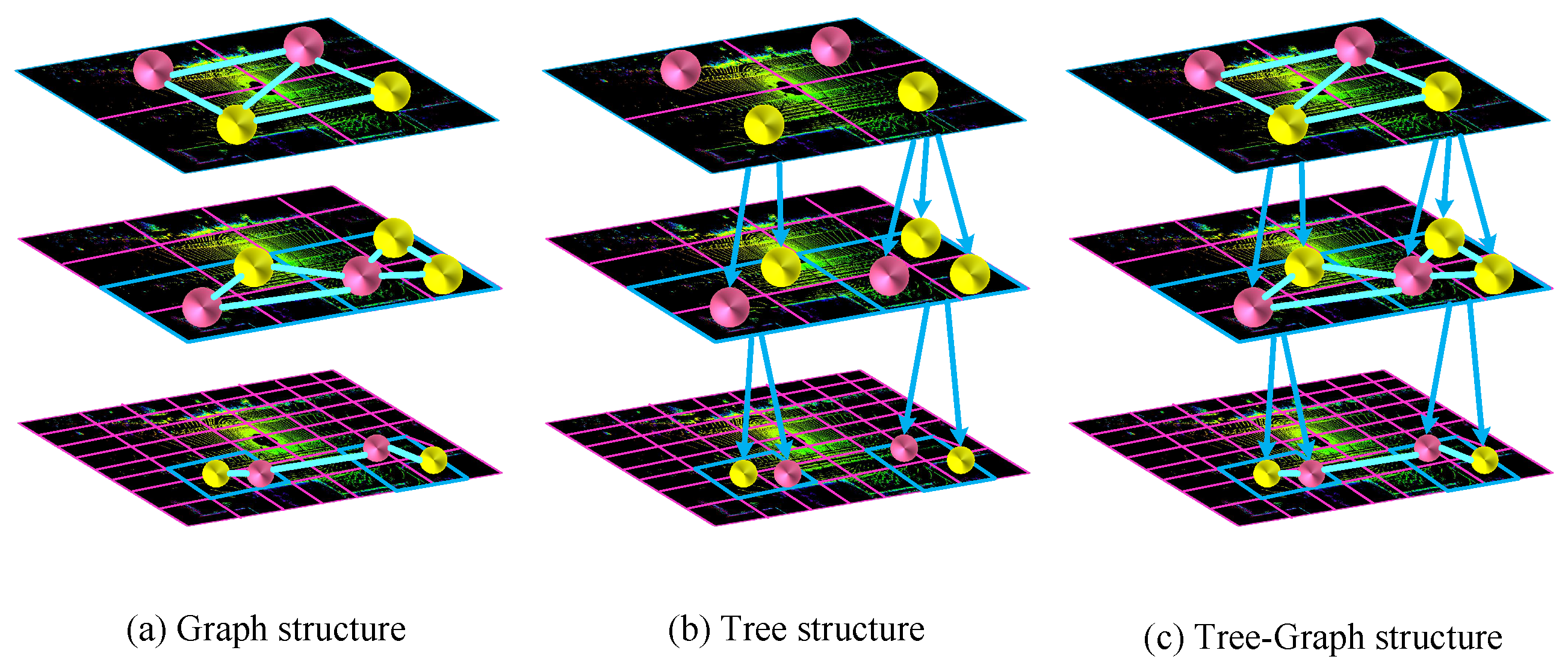
To address these challenges, recent methods primarily adopt either graph-based or tree-based representations. Graph-based methods [9,10,11,12] construct local neighborhoods via spatial proximity, effectively capturing fine geometric details and local variations, as shown in Figure 1a. Most use fixed-radius or k-nearest neighbor (KNN) strategies [13,14], which assume uniform point distributions. This assumption makes them sensitive to point density variations—leading to information loss in sparse regions and noisy redundancy in dense ones [15]. In contrast, tree-based approaches [16,17] exploit hierarchical structures through progressive downsampling to efficiently capture multi-scale global semantics, as shown in Figure 1b. However, such coarse-to-fine hierarchies can discard crucial local details, and static tree structures often lack adaptability to irregular spatial layouts [18]. These two paradigms exhibit complementary advantages: Graph-based models excel at local geometric encoding, while tree-based models are better suited for global semantic reasoning. Nonetheless, existing methods typically treat them in isolation, missing opportunities for joint optimization.
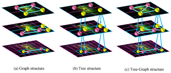
Figure 1.
Illustration of the different structures of point cloud data. (a) Graph structure captures local neighborhoods through edges between nodes but has limited global representation. (b) Tree structure provides hierarchical organization and multi-scale analysis but may be lacking in local detail capture. (c) Tree–graph structure combines the strengths of both, enabling the effective integration of local and global features through bidirectional message passing.
Recent efforts have improved graph construction and hierarchical aggregation independently [7,13], but two core limitations persist: (1) hierarchical downsampling often leads to local information loss and semantic gaps across scales; (2) there is limited interaction between local graph-based features and global tree-based context, restricting the expressive capacity of hierarchical feature learning.
Inspired by the theoretical framework of Hierarchical Support Graphs (HSGs) [19], we argue that integrating hierarchical (tree) structures with graph-based message passing can significantly enhance feature learning. Specifically, the multi-level structure combined with cross-message passing effectively reduces path resistance within the graph, thereby improving connectivity and facilitating more efficient information flow.
Therefore, we propose a novel framework: density-aware tree–graph cross-message passing for LiDAR-based 3D object detection. Our method integrates the complementary strengths of graph and tree structures to achieve both local fidelity and global context understanding. Specifically, we introduce a density-aware graph construction module that dynamically incorporates local density cues when forming neighborhoods, enabling more robust feature extraction in non-uniform regions. We then design a hierarchical tree representation module to encode multi-scale semantics while preserving spatial consistency, as shown in Figure 1c. To bridge the local–global gap, we propose a tree–graph cross-message-passing mechanism, which facilitates bi-directional feature interactions between the graph and tree branches. This design leads to stronger feature expressiveness, as it enables both precise local encoding and robust global context reasoning through complementary interactions between tree and graph representations.
In summary, the main contributions of this work are summarized as follows:
- The DAGC strategy adaptively builds local neighborhoods by considering spatial proximity and local point density, thus avoiding redundant connections in dense regions and maintaining connectivity in sparse areas.
- HTR models multi-scale semantic features through structured downsampling, preserving the global context while being aware of spatial structure.
- The TGCMP mechanism enables bi-directional feature exchange between graph and tree domains, allowing local geometric patterns and global semantic cues to reinforce each other.
2. Related Works
2.1. Overview of LiDAR-Based Methods
Voxelization is a common approach that transforms irregular point clouds into structured grids, enabling 3D convolutional processing. Early methods like VoxelNet [20] pioneered end-to-end voxel feature encoding but incurred high computational costs. Subsequent works—including SECOND [21], PointPillars [22], Part- [23], Voxel-RCNN [24], HVNet [25], and CIA-SSD [26]—have focused on improving efficiency and accuracy by leveraging sparse convolutions, pseudo-BEV representations, multi-scale feature extraction, and confidence-aware refinement. VoTr [27] introduces transformers to better model contextual dependencies, addressing the locality bias of traditional CNNs. Swin3D [28] introduces a generalized contextual relative positional embedding mechanism to capture various irregularities in point cloud signals while enabling efficient self-attention on sparse voxels, thereby allowing the model to scale to larger sizes and datasets.
Point-based detectors operate directly on raw point clouds to preserve detailed geometric structures. Point-RCNN [29] applies PointNet++ [30] for hierarchical feature learning and two-stage refinement. To improve efficiency, 3DSSD [31] and IA-SSD [32] utilize progressive downsampling and fusion schemes to retain informative foreground points with reduced overhead. STD [33] introduces a point-level proposal generation mechanism with spherical anchors to enhance object recall. Point-GNN [9] formulates detection as a graph reasoning problem, aligning features to point positions via graph neural networks.
To harness both fine-grained point features and the global voxel context, hybrid approaches have gained popularity. SA-SSD [34] incorporates auxiliary supervision to enrich voxel features with point-level cues. PV-RCNN [35] introduces a voxel-set abstraction mechanism to project voxel features to keypoints, achieving fine-to-coarse information fusion. CT3D [36] leverages channel-wise transformers to model inter-channel geometric relationships, and Pyramid-RCNN [37] proposes a scale-adaptive spherical query strategy to enhance RoI feature coverage.
2.2. Methods Based on Graph Network
Graph neural networks (GNNs) have become an increasingly influential framework for processing 3D point clouds, thanks to their ability to handle irregular, unordered data and model complex geometric relationships. Unlike convolutional operations on structured grids, GNNs naturally encode local topology and inter-point dependencies, making them well-suited for point cloud representation learning [10,38,39,40]. To better capture local spatial interactions, Point-GNN [9] constructs hierarchical graphs from point clouds and performs feature propagation along edges, followed by graph-aware NMS to improve proposal refinement. DRG-CNN [12] dynamically builds neighborhood graphs per layer, allowing receptive fields to adaptively expand and enabling more flexible context encoding. SVGA-Net [41] introduces voxel-guided multi-scale graph construction and leverages attention mechanisms to selectively fuse geometric features across scales. DGT-Det3D [18] further combines graph reasoning with semantic-aware modules, enhancing both the structural and contextual aspects of point features. Collectively, these graph-based approaches demonstrate the strength of GNNs in learning fine-grained geometric representations and neighborhood-aware context, contributing to more accurate and robust 3D object detection.
2.3. Methods Based on Multi-Scale Feature Learning
Existing multi-scale feature learning methods, such as FPN-based architectures [42], PointNet++ [30], hybrid voxel encoders [25], and KD-Net [43], have advanced 3D detection by hierarchically aggregating features at different resolutions. However, they often process local and global contexts separately or lack adaptability to non-uniform density and irregular geometry. Recent adaptive hierarchies improve flexibility but still underexploit cross-scale interactions. To bridge this gap, we propose a tree–graph cross-message-passing mechanism that enables bi-directional interactions between hierarchical (tree-based) and local geometric (graph-based) features, unifying fine-grained detail preservation with global semantic reasoning for enhanced multi-scale 3D representation.
2.4. Transformer-Based 3D Object Detection Methods
The introduction of Transformers [44] has fundamentally reshaped 3D visual understanding by enabling long-range dependency modeling via self-attention mechanisms. Inspired by their breakthroughs in 2D computer vision—such as the Vision Transformer (ViT) [45,46], DETR [47], and Swin Transformer [48]—researchers have actively explored their extensions to the 3D domain. In 3D perception, Point-BERT [49] pioneers masked point modeling for unsupervised pretraining, treating point clouds as tokenized sequences and effectively capturing global semantics. Other approaches, like Point Transformer [50], propose coupling the strengths of attention mechanisms with local geometric priors, enabling precise context aggregation at both fine and coarse levels. DVST [51] integrates deformable voxel-set attention into a Transformer backbone to adaptively aggregate informative regions and enhance 3D object detection from LiDAR point clouds. Meanwhile, FusionRCNN [52] effectively fuses LiDAR geometric information and camera texture information through cross-modal attention, achieving more precise feature complementarity and enhancement, which significantly improves multi-modal 3D object detection performance. SGF3D [53] applies cross-modal attention modules to bridge modality gaps and improve fusion consistency in multi-sensor scenarios. These transformer-inspired architectures have advanced the state of the art across key 3D tasks, including object classification, semantic segmentation, and 3D detection, by bridging local detail preservation with global feature reasoning.
3. Methodology
3.1. The Overview of Our Method
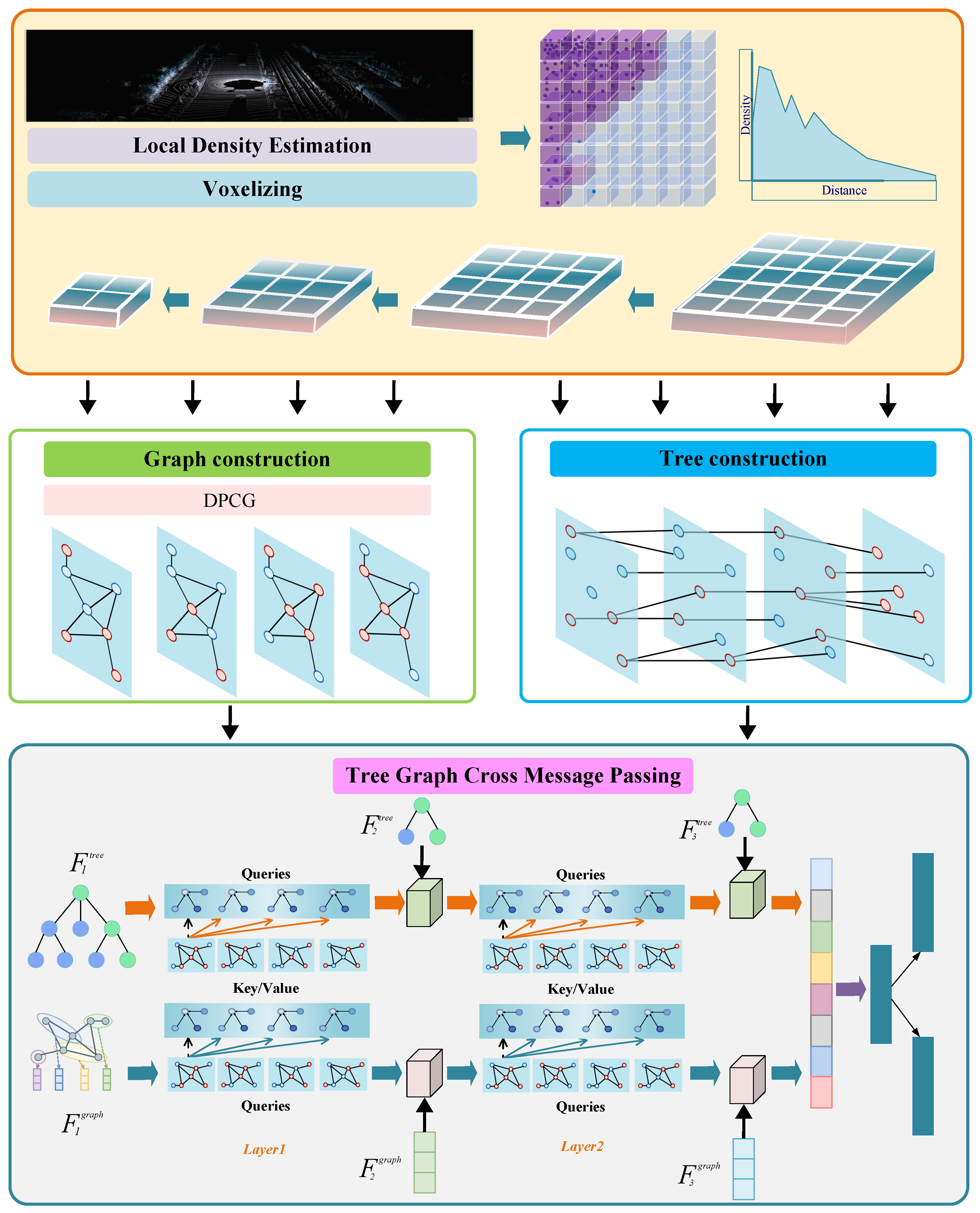
The pipeline of DA-TGCMP is shown in Figure 2. The framework consists of four main stages. Initially, voxelization combined with local density estimation is employed to capture the inherent spatial non-uniformity of the point cloud. DPCG is then constructed to enhance local neighborhood modeling, especially in sparse regions. Subsequently, a hierarchical tree representation module is introduced to encode multi-scale semantic features in a structured and spatially aware manner. To bridge local and global representations, the TGCMP mechanism is developed, enabling bidirectional feature exchange between the tree and graph views. This unified design facilitates expressive hierarchical feature learning by integrating fine-grained geometric cues with high-level semantics, ultimately leading to more robust and accurate 3D detection.

Figure 2.
Architecture of the proposed DA-TGCMP framework for LiDAR-based 3D object detection. The framework comprises four stages: (1) density-aware voxelization, where local point densities are estimated to reflect spatial variation; (2) graph construction using the proposed DPCG strategy to build robust local neighborhoods; (3) hierarchical tree construction via structured downsampling to capture multi-scale semantic context; and (4) tree–graph cross-message passing, which enables bi-directional feature interaction between tree and graph representations for enhanced feature learning.
3.2. Local Density Estimation
In 3D point cloud processing, the inherent non-uniformity in point distributions arises due to various factors such as sensor limitations, occlusions, and varying distances from the sensor to objects. This results in the phenomenon of dense regions near the sensor and sparse regions farther away, which introduces significant challenges for effective local feature extraction. Traditional methods that rely on fixed-radius or fixed-k neighborhood queries often fail to adapt to these density variations, which may lead to suboptimal performance in downstream tasks.
To address this issue, we propose a novel local density estimation (LDE) module that explicitly models local density variations, enabling more adaptive and robust feature extraction. Given a point cloud , where each point represents a 3D coordinate, the first step is to identify the local neighborhood for each point. This is achieved by performing search, which selects the k closest points to each point . Formally, for each point , we define the neighborhood as a set of its KNN:
The KNN search strategy ensures that each point has a fixed number of neighbors, which provides a consistent basis for subsequent density estimation, irrespective of the point’s position in the point cloud. Compared to fixed-radius approaches, this method offers a more stable representation, particularly in point clouds with significant density variations. Once the local neighborhood for each point is established, the next step is to estimate the local density for each point using Kernel Density Estimation (KDE). KDE provides a smooth and continuous estimate of the local density by assigning weights to the neighboring points based on their distances from . The KDE for point is given by
where denotes the Euclidean distance between points and , and is the bandwidth parameter that controls the kernel’s spread. This kernel function ensures that closer neighbors contribute more significantly to the density estimate than more distant neighbors, which allows for fine-grained local density modeling.
To further enhance the density estimation process, we introduce an adaptive bandwidth strategy that dynamically adjusts bandwidth based on the local distribution of points. The bandwidth is computed as the average distance between the point and its k nearest neighbors:
This adaptive strategy ensures that in dense regions, the kernel bandwidth is smaller (i.e., the kernel becomes more concentrated around each point), while in sparse regions, the kernel bandwidth becomes larger. This adaptability allows the method to better handle point clouds with varying density, ensuring that the kernel can effectively capture local structures regardless of the region’s sparsity or density. After estimating the local densities, we perform a density normalization step to rescale the density values to a consistent range. This normalization step is crucial for enabling meaningful comparisons between points across point clouds with varying global densities. The normalized density for each point is computed as follows:
where and are the minimum and maximum density values across the entire point cloud, respectively. This normalization step ensures that the local density values are rescaled to the range , providing a uniform density scale across point clouds with different global density distributions. Finally, based on the normalized density values, we partition the point cloud into dense and sparse regions. Points with are classified as part of a dense region, while points with are classified as part of a sparse region. The thresholds and can either be manually defined or adaptively determined based on the statistical properties of the density distribution, such as the quantiles of the density values. This step enables the segmentation of the point cloud into regions that exhibit similar density characteristics, allowing for region-specific processing strategies in subsequent steps. For example, in dense regions, fine-grained feature extraction can be performed, whereas in sparse regions, broader receptive fields may be required to capture important structures.
3.3. Dynamic Point Cloud Grouping
To effectively capture local geometric structures in point clouds, we propose a novel method termed dynamic point cloud grouping (DPCG). As shown in Algorithm 1, by integrating local density indices with adaptive distance thresholds, DPCG enables efficient point cloud segmentation and feature aggregation. The dynamic distance threshold for each point is defined as follows:
where and denote the minimum and maximum distance thresholds, respectively. Typically, is set to a small value (e.g., 0.1) to capture fine-grained structures in high-density regions, while is assigned a larger value (e.g., 0.5) to ensure robust grouping in sparse areas. This dynamic adjustment balances the trade-off between geometric fidelity and computational efficiency.
Grouping is performed using a breadth-first search (BFS) strategy. At each iteration, the ungrouped point with the highest density is selected as the seed . A queue is initialized with , and points are iteratively dequeued to explore their unvisited neighbor . A neighbor is added to the current group if the distance is less than its adaptive threshold . The process repeats until the queue is empty. New groups are initialized by selecting the next highest-density ungrouped point, and the procedure continues until all points are assigned to groups.
| Algorithm 1 Dynamic Point Cloud Grouping (DPCG) |
|
3.4. Density Graph Construction
Dynamic point cloud grouping enables adaptive neighborhood formation, but conventional graph construction often overlooks underlying density variations. This can result in missing fine-grained patterns in sparse areas or overemphasizing redundant information in dense regions.
To address this, we propose a density graph construction strategy that integrates local density cues for more reliable graph formation. This enhances geometric structure preservation and facilitates robust local feature extraction across varying density regions.
Formally, given a point cloud with coordinates and features , we define nodes as
For each node , we estimate an adaptive radius and define its neighborhood:
The adjacency matrix A encodes these relationships, with if . The edge features are
where is a learnable transformation (e.g., MLP).
Node features are projected for attention computation:
with the following attention scores:
The updated node features are
This density-aware graph enables effective local feature learning by jointly modeling semantic and geometric relationships across variable-density regions.
3.5. Hierarchical Tree Representation
We introduce a novel hierarchical tree representation during the point cloud downsampling process to effectively organize points at multiple scales. Given a single-frame point cloud , where N is the number of points and each point consists of 3D coordinates, we progressively construct a tree hierarchy. At each layer, the point cloud is represented at a coarser resolution by dividing the 3D space into cubic voxels. The centroid of each voxel acts as the parent node of the tree, enabling multi-scale feature extraction and efficient attention aggregation.
3.5.1. Voxel Grid Construction and Parent–Child Mapping
To build the tree, the 3D space is partitioned into a voxel grid at each layer. For each voxel , we compute its centroid , which serves as the representative point for that voxel. At the coarsest level , the centroids directly correspond to the input points of the point cloud X, acting as the leaf nodes of the tree. As we move to finer layers l, the voxel size increases, representing a coarser version of the point cloud. Each centroid at the finer layer is mapped to a parent voxel at the coarser layer, forming the tree hierarchy.
Let represent the set of voxels at layer l, where each voxel contains a subset of points. The centroid of a voxel at layer l is computed by averaging the coordinates of the points within that voxel:
where is the set of points in the i-th voxel at layer l, and is the number of points in that voxel.
3.5.2. Parent–Child Relationship and Layer-Wise Indexing
The essence of the tree construction lies in mapping the parent and child nodes across layers. For each child point in a finer layer, we define the index that maps it to its parent point in the coarser layer:
where is a point in the finer layer, and is the voxel containing . Conversely, for each parent point at layer l, the set of child points in the next layer is defined as
where is the voxel containing the parent point at layer l.
The voxel size at each layer l increases according to
where is the initial voxel size, N is the scaling factor, and l is the layer index. As l increases, the voxel’s size grows, leading to progressively coarser representations of the point cloud.
3.5.3. Coarse-Level Node Computation
At each layer, the parent node’s coordinates are computed as the average of the child nodes’ coordinates:
where is the centroid of the i-th parent node at the coarser level, is the set of indices for the child points at the finer level, and is the coordinate of the j-th child point.
This tree construction process continues until we obtain a multi-layered tree, where the leaf nodes represent the fine-grained point cloud X, and the root node represents the coarsest point representation. As shown in Algorithm 2, this tree structure facilitates efficient feature aggregation across scales, enabling effective point cloud representation learning.
| Algorithm 2 Tree Construction for Point Cloud Downsampling |
|
3.6. Tree–Graph Cross-Message Passing
In hierarchical point cloud processing, downsampling is essential for building multi-scale representations but inevitably causes the loss of fine-grained local structures. Density-aware graphs provide a way to preserve local geometric and semantic relationships; however, they often suffer from information degradation across hierarchical levels. On the other hand, tree structures, constructed in a dense-to-sparse manner, effectively retain global contextual cues but are less sensitive to local variations. By drawing inspiration from the theoretical framework of hierarchical support graphs (HSGs) [19], to bridge the gap between local precision and the global context, we propose a TGCMP mechanism, which enables bi-directional feature interaction between tree and graph representations, leading to more expressive hierarchical feature learning. TGCMP implicitly increases the number of node-disjoint paths between node pairs through the integration of tree and graph structures. This design is analogous to how the vertical and horizontal edges in HSGs enhance graph connectivity and facilitate more robust information exchange. Specifically, TGCMP comprises the following components:
- The tree features at level l as , where is the number of nodes and D is the feature dimension.
- The graph features at level l as .
- The 3D coordinates of nodes as .
3.6.1. Top-Down Message Passing (Tree → Graph)
The top-down branch aims to inject global contextual information from the tree structure into the local graph features at the same level l. First, the tree feature of node i is projected into a query vector:
where is a learnable weight matrix, and d denotes the query dimension. Similarly, the graph features are projected into keys and values:
where denotes learnable parameters. To encode spatial relationships, we compute a relative positional encoding:
where is a lightweight neural network, such as an MLP, that maps relative coordinates into feature space. The attention weight between a tree node i and a neighboring graph node is computed as follows:
The aggregated message at node i is computed by applying an attention-weighted aggregation over its neighbors:
where denotes the transformed features of neighboring graph nodes, and denotes the attention weights. The updated feature at node i is then obtained by combining its original feature with the aggregated message using a residual connection followed by a multilayer perceptron (MLP):
This design provides several theoretical advantages:
- Enhanced connectivity: Cross-layer aggregation increases node-disjoint paths:thus alleviating over-squashing and improving message robustness.
- Reduced effective resistance: Cross-layer connections reduce the effective resistance between node pairs:leading to more efficient long-range communication.
- Expanded receptive field: The tree-to-graph cross-message passing expands the receptive field logarithmically without increasing the network’s depth:
These properties ensure that top-down message passing provides both global context injection and computational efficiency.
3.6.2. Bottom-Up Message Passing (Graph → Tree)
The bottom-up branch aggregates fine-grained local features from graph nodes and propagates them to their corresponding parent tree nodes.
Let denote the set of child graph nodes associated with a tree node i. The feature of the parent node is updated as follows:
where denotes feature concatenation, and the MLP learns to adaptively combine the child features with their relative positional offsets.
3.7. Loss Functions
Our network is structured as a two-stage detector and optimized by a unified multi-task loss that concurrently supervises the RPN and R-CNN stages.
Following [23], the RPN loss consists of object classification loss, box regression loss, and corner regression loss:
where , , and are weighting coefficients. The classification loss is computed using the focal loss [54]:
where is the predicted objectness score, and and are hyperparameters. The box regression loss employs the Smooth L1 loss [55] over the encoded box residuals:
where the residuals are defined as
with . The corner loss is computed based on the sine error [21] between the predicted and ground truth box corners. In the refinement stage, supervises the region-of-interest (ROI) heads by optimizing classification, bounding box regression, and corner prediction:
Here, is the cross-entropy loss for classification, is the Smooth L1 loss for box regression, and is the sine-based corner loss.
4. Experiment
4.1. Datasets and Evaluation Metric
To comprehensively evaluate the performance of our proposed DA-TGCMP method, we conduct experiments on three large-scale LiDAR-based 3D object detection benchmarks: KITTI, nuScenes, and Waymo Open Dataset. These datasets vary in complexity, sensor settings, and evaluation metrics, thus enabling a holistic assessment.
The KITTI dataset is one of the earliest and most widely adopted benchmarks for 3D detection. We follow the standard evaluation protocol that partitions the official 7481 LiDAR scans into a training set (3712 samples) and a validation set (3769 samples), ensuring minimal sequence overlap to maintain evaluation fairness. The detection range is constrained within [0 m, 70.4 m] along the X-axis, [−40 m, 40 m] along the Y-axis, and [−3 m, 1 m] along the Z-axis in the LiDAR coordinate frame. KITTI defines evaluation difficulty levels—easy, moderate, and hard—based on object size, occlusion, and truncation, with performance reported using average precision (AP) under the 40 recall position metrics.
The nuScenes dataset introduces a more challenging urban scenario, offering 1000 driving scenes captured at 2 Hz and covering diverse weather, lighting, and traffic conditions. It includes 700 scenes for training, 150 for validation, and 150 for testing. Rich annotations span 23 object categories and are aligned across multiple modalities, including LiDAR, cameras, and radar. Detection performance is assessed using both the mean average precision (mAP) and the nuScenes detection score (NDS), the latter being a compound metric accounting for classification, translation, scale, orientation, velocity, and attribute estimation.
The Waymo Open Dataset is known for its dense and high-fidelity point cloud data, capturing 360° environments with a fine voxel resolution of 0.1 m, 0.1 m, and 0.15 m. It comprises 798 training sequences (around 158,000 frames) and 202 validation sequences (around 40,000 frames). The detection space spans from −75.2 m to 75.2 m in both X and Y directions and from −2 m to 4 m vertically. For fair evaluation, Waymo differentiates predictions into LEVEL_1 (≥5 LiDAR points) and LEVEL_2 (≥1 LiDAR point). The metrics used include the standard mean average precision (mAP) and its orientation-sensitive variant mAPH, which reflects heading prediction quality.
4.2. Implementation Details
Recent works [21,22,33,35] used 11 recall positions to calculate average precision (AP) on the validation set, while the KITTI benchmark adopts 40 recall positions for the test set. We follow this approach, using 40 recall positions for the test set and 11 for the validation set. For consistency, we train DA-TGCMP on the complete set of KITTI training samples when providing submissions to the KITTI test benchmark.
For region proposal generation, we downsample the sparse voxel tensor by factors of 1×, 2×, 4×, and 8×. The voxel feature tensor sizes are set to [16, 32, 64, 64] at each scale. We place six anchors at each pixel of the BEV feature map for three categories, each with two heading angles, and compute pixel features for both classification and box regression tasks.
We use 3D average precision (3D AP) and bird’s-eye-view average precision (BEV AP) as our performance metrics. Training follows standard practices with an Adam optimizer [56], a weight decay of 0.01, and a momentum of 0.9, and we use over 70 epochs with an initial learning rate of 0.003. During inference, we apply non-maximum suppression (NMS) with a threshold of 0.7 to filter out redundant proposals and keep the top 100 for input into the refinement module.
5. Results and Analysis
5.1. Comparison on the KITTI Test Set
Table 1 summarizes the quantitative performance of DA-TGCMP on the KITTI 3D detection test set across three object categories, car, pedestrian, and cyclist, evaluated under easy, moderate, and hard settings. The results show that DA-TGCMP achieves the highest AP scores among all listed methods in the car category: 91.01% (easy), 83.56% (moderate), and 79.14% (hard). Compared to previous leading methods such as PVT-SSD (90.65%, 82.29%, and 76.85%) and PV-RCNN (90.25%, 81.43%, and 76.82%), the proposed method shows moderate yet consistent improvements, particularly under the moderate and hard settings, suggesting the effective handling of challenging driving scenes. For the pedestrian category, DA-TGCMP reaches AP scores of 53.53% (easy), 47.92% (moderate), and 45.96% (hard). These results are marginally better than existing voxel-based methods such as VoFiNet (53.07%, 47.43%, and 45.22%) and HVPR (53.47%, 43.96%, and 40.64%), indicating slight gains in detecting small-scale or occluded pedestrian objects. However, the improvements are relatively limited, suggesting that the detection of pedestrians remains a challenging task even for advanced methods. In the cyclist category, DA-TGCMP achieves 81.62% (easy), 67.15% (moderate), and 61.73% (hard). These values are close to or slightly above the best-performing baselines, such as VoFiNet (77.64%, 64.10%, and 58.00%) and Part-A² (79.17%, 63.52%, and 56.93%), indicating competitive performance. The gains are more pronounced under higher difficulty levels, reflecting the method’s robustness when facing occlusion or limited point density. Overall, DA-TGCMP demonstrates better performance across all categories, particularly excelling in the car detection task. The relatively smaller margins in pedestrian and cyclist detection suggest room for further improvement, particularly in handling fine-grained localization under occlusion.

Table 1.
Performance comparison of the KITTI test set. The results are reported by the AP and 40 recall points.
5.2. Comparison on the nuScenes Test Set
The DA-TGCMP algorithm demonstrates exceptional performance on the nuScenes 3D detection test set shown in Table 2, as evidenced by its high mean average precision (mAP) of 66.6 and NuScenes detection score (NDS) of 71.7. These scores indicate that the algorithm can effectively detect various objects in complex traffic scenarios, providing a robust foundation for 3D object detection tasks. Car Detection: With an accuracy of 86.9, DA-TGCMP excels in detecting cars, which are the most common objects in traffic scenarios. This high accuracy ensures the reliable detection of primary road users, which is crucial for autonomous driving safety. Pedestrian Detection: Achieving an accuracy of 86.9, the algorithm also performs outstandingly in identifying pedestrians. Given the complexity and variability of human shapes and poses, this result highlights the algorithm’s strong feature extraction and generalization capabilities. Construction Vehicle (C.V.) Detection: Achieving an accuracy of 32.1, the algorithm can manage the complex shapes of construction vehicles. Although there is room for improvement, this accuracy reflects its capability to detect these less common but important objects in specific environments. Traffic Cone (T.C.) Detection: At 82.3, the algorithm demonstrates good performance in detecting traffic cones. Their unique shape is effectively captured by the algorithm, aiding in road guidance and obstacle avoidance. Compared to other methods, DA-TGCMP shows competitive performance across most categories. It performs particularly well in car and pedestrian detection, indicating its strength in handling common and complex traffic participants. However, there is room for improvement in detecting objects like bicycles and motorcycles.
Table 2.
Performance comparison of the nuScenes 3D detection test set. C.V, Motor., Ped., and T.C. are abbreviations for construction vehicle, motorcycle, pedestrian, and traffic cones, respectively.
5.3. Comparison on Waymo Validation Set
As detailed in Table 3, we validate the multi-class detection results of the Waymo Open Dataset. The DA-TGCMP algorithm exhibits remarkable performance on the Waymo Open Dataset. Specifically, in vehicle detection, it attains a LEVEL_1 mAP of 76.64, marking a 4.37% improvement over SECOND’s 72.27 and a substantial 20.02% enhancement compared to PointPillars’ 56.62. In pedestrian detection, the LEVEL_1 mAP of 74.46 represents a 15.21% improvement relative to PointPillars’ 59.25. Moreover, for cyclist detection at LEVEL_2, it achieves an mAPH of 64.78, surpassing PointPillars’ 58.34 by 6.44%. In vehicle detection, it achieves a high LEVEL_1 mAP and a LEVEL_2 mAPH of 76.69, outperforming CenterPoint (72.15) and VoTr-TSD (74.95) by 4.49% and 1.69%, respectively. For pedestrian detection, it demonstrates robust performance at both difficulty levels, achieving a LEVEL_1 mAP of 74.46, which underscores its effective handling of challenges such as diverse poses and occlusions. In cyclist detection, while the LEVEL_1 mAP is slightly lower than some methods, the LEVEL_2 mAPH of 64.78 indicates the efficient detection of dynamic cyclists. In pedestrian detection at LEVEL_1, it outperforms CenterPoint (69.04) and VoTr-TSD (71.36) by a significant margin. These results highlight DA-TGCMP’s effectiveness in managing complex traffic scenes with high accuracy and good generalization.
Table 3.
Performance comparison on the Waymo Open Dataset with 202 validation sequences for 3D vehicle (IoU = 0.7), pedestrian (IoU = 0.5), and cyclist (IoU = 0.5) detection.
5.4. Ablation Studies
In this section, we perform an ablation study to evaluate the contribution of key components in the DA-TGCMP framework. The main goal is to investigate how each individual module impacts the overall performance of our model in the task of LiDAR-based 3D object detection.
5.4.1. Effect of Each Module
The baseline model provides a robust foundation for 3D object detection, achieving strong performance across both the KITTI and nuScenes datasets. As detailed in Table 4, On the KITTI dataset, the baseline model achieves 91.19%, 82.63%, and 82.01% in the easy, moderate, and hard categories, respectively. On the nuScenes dataset, the model records an NDS of 65.4 and a mean average precision (mAP) of 0.592. These results demonstrate the baseline’s ability to effectively capture the key features required for accurate 3D object detection, establishing it as a strong starting point for further enhancements.
Table 4.
Results of the proposed DAGC, HTR, and TGCMP modules on the KITTI and nuScenes validation sets.
Integrating the DAGC module with the baseline model leads to significant performance improvements, especially in the moderate and hard categories on KITTI. The model achieves 84.86% and 82.61% in these categories, respectively, compared to the baseline’s 82.63% and 82.01%. This demonstrates DAGC’s ability to address varying point densities within LiDAR point clouds by dynamically adapting the graph’s structure. The improved results highlight DAGC’s effectiveness in enhancing feature extraction, particularly in complex scenarios where point cloud density varies. Additionally, on the nuScenes dataset, the model shows slight increases in both NDS and mAP, further confirming DAGC’s role in improving feature representation.
The addition of the hierarchical tree representation (HTR) further refines the model’s ability to capture multi-scale semantic features. While the improvement in the easy category on KITTI is marginal, the model experiences notable gains in the moderate and hard categories, with 84.24% and 82.24%, respectively, compared to the baseline’s 82.63% and 82.01%. This indicates that HTR enhances the model’s ability to preserve global context and capture multi-scale features through its structured downsampling approach. These improvements are also reflected in a slight increase in NDS on the nuScenes dataset, further demonstrating the effectiveness of hierarchical downsampling in strengthening the model’s performance.
When combining DAGC and HTR with the tree–graph cross-message-passing (TGCM) module, the model experiences the most significant performance improvements. On KITTI, the model achieves 92.52%, 86.87%, and 82.59% for the easy, moderate, and hard categories, respectively, a substantial improvement over the previous configurations. Similarly, on nuScenes, the model records an NDS of 68.1 and an mAP of 0.630, further emphasizing the importance of TGCM. This module facilitates bi-directional feature interaction between the graph and tree structures, enabling the model to effectively aggregate local features with the global context. The enhanced feature learning process through cross-message passing results in significant boosts across all performance metrics on both datasets.
Each module contributes uniquely to the performance improvements observed in the experimental results: DAGC proves to be highly effective in handling varying point densities within LiDAR point clouds. Its adaptive graph construction allows the model to better capture geometric structures, especially in the moderate and hard categories of KITTI. This improvement is crucial for preserving relationships across regions with varying densities and ensuring robust feature extraction.
HTR strengthens the model’s ability to capture global context and multi-scale semantic features. The structured downsampling approach of HTR helps preserve crucial global information, as demonstrated by the improved performance across different difficulty levels on KITTI and the enhanced NDS on nuScenes.
TGCMP stands out as the most impactful module, refining local features and effectively aggregating global context through cross-message passing between tree and graph representations. This dual enhancement significantly boosts performance across all metrics on both datasets, demonstrating the importance of incorporating both local and global feature interactions.
5.4.2. Effect of DAGC
To further validate the effectiveness of the proposed density-aware graph construction (DAGC) module, we conduct a comparative study against two widely used neighborhood construction strategies, fixed-radius and kNN, on the KITTI dataset. The evaluation spans three object categories—car, pedestrian, and cyclist—across all standard difficulty levels (easy, moderate, and hard).
DAGC consistently achieves the highest accuracy across all difficulty levels. In particular, as follow in Table 5, it exhibits substantial gains in the moderate and hard categories, which typically involve cluttered scenes or partially occluded vehicles. These improvements highlight DAGC’s ability to construct more informative graph structures that better capture the local geometric variations in sparse or complex regions.The performance of DAGC surpasses both fixed-radius and KNN methods, with notable advantages in the hard category. Pedestrian detection in this category is challenging due to factors such as occlusion and long-range perception. The superior results of DAGC suggest that its density-adaptive neighborhood construction enables the more effective representation of pedestrians under such adverse conditions. DAGC also leads in the easy and hard categories for cyclist detection. The improvements in the hard setting reflect the module’s robustness in handling ambiguous or incomplete point cloud inputs, while the gains in the easy setting demonstrate that even in less complex scenarios, DAGC facilitates more accurate feature extraction compared to traditional methods.
Table 5.
Effects of DAGC module, fixed-radius, and kNN for DA-TGCMP. Results on the KITTI val set for car, pedestrian, and cyclist classes.
5.4.3. Effect Between Dense and Sparse Regions
As shown in Table 6, our proposed DA-TGCMP consistently demonstrates superior performance in small-object detection across both dense and sparse regions. Specifically, on the KITTI dataset, DA-TGCMP achieves a notable 92.38 mAP for bicycles (Cyc) in dense regions and 17.36 mAP in sparse regions (IoU = 0.5), outperforming competitive baselines such as PointGNN and VoxelGraph-RCNN by a substantial margin. This corresponds to a 68% relative improvement in sparse-region small-object detection compared to the best alternative method.
Table 6.
Performance comparison on KITTI dataset across dense and sparse regions.
Crucially, DA-TGCMP exhibits remarkable resilience against sparsity-induced performance degradation. While existing baselines suffer severe accuracy declines in sparse regions (e.g., PointGNN’s Cyc mAP drops by 91.9% from dense to sparse regions), DA-TGCMP significantly mitigates this effect, reducing the performance drop by 10.7 percentage points and achieving a retention rate of 81.2%. These results underline the effectiveness of our dynamic graph convolution in preserving discriminative features in challenging sparse environments.
5.4.4. Effect of Different Dynamic Radius Designs
We systematically evaluate the impact of different dynamic distance threshold designs on small-object detection performance, as shown in Table 7. The fixed-radius method performs relatively poorly (56.21 AP) due to its inability to adapt to variations in point cloud density. In contrast, the density-aware linear adjustment strategy significantly improves detection accuracy (60.82 AP), indicating that adapting to local sparsity enables more effective feature aggregation. Further incorporating nonlinear adjustment functions, the exponential form () demonstrates better inclusiveness in sparse regions and achieves 61.47 AP, outperforming the logarithmic form (59.35 AP), which responds more slowly to density changes. Moreover, broadening the threshold range (from 0.05 to 0.6) enhances the ability to capture structures in sparse regions while maintaining accuracy in dense areas, leading to 62.03 AP. The best performance (63.40 AP) is achieved using an MLP-based strategy to learn adaptive thresholds, suggesting that data-driven threshold learning combining semantic and structural cues is a promising direction for future research.
Table 7.
Effect of different dynamic radius designs of small-object (pedestrian) detection on KITTI Val.
As shown in Figure 3, the BEV visualization reveals the effectiveness of our dynamic point cloud processing pipeline. Figure 3a displays the rasterized point cloud density distribution. Red points depict the spatial arrangement of point clouds after rasterization, reflecting the raw density characteristics of the scene. From Figure 3b, this adaptive clustering reorganizes sparse point cloud data into semantically meaningful groups, facilitating downstream tasks like object detection and segmentation.
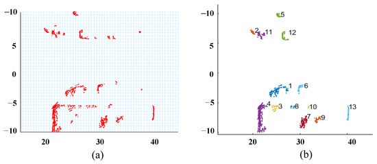
Figure 3.
Bird’s eye view (BEV) of point cloud feature. (a) The point cloud density distribution after rasterization. (b) The result of dynamic point cloud grouping.
5.4.5. Effect of Tree Structure
To evaluate the contribution of hierarchical tree structure to point cloud representation, we conduct a comparison with two baseline methods, single-scale voxel aggregation and PointNet-style global pooling, as shown in Table 8. In our experiments comparing single-scale voxel aggregation, PointNet-style global pooling, and the proposed hierarchical tree structure, the results demonstrate that the tree structure outperforms the other methods across all metrics and datasets. Single-scale voxel aggregation performed decently on simpler scenarios but struggled with complex cases, as it fails to capture multi-scale features. PointNet-style global pooling showed slight improvements over voxel aggregation, particularly in more complex scenarios, but still lacked the effective handling of multi-scale information. Hierarchical tree structure consistently outperformed the other methods, achieving the highest accuracy on both KITTI and nuScenes. Its ability to capture multi-scale relationships and hierarchical structures contributed to its superior performance, especially in challenging scenarios. Overall, the hierarchical tree structure proves to be the most effective in handling diverse 3D object detection tasks, particularly by leveraging multi-scale feature aggregation and hierarchical relationships, which are crucial for complex, real-world applications.
Table 8.
Results on the KITTI and nuScenes validation sets using different baseline methods.
5.4.6. Effect of TGCMP
To validate the effectiveness of our method, we design a series of ablation experiments focusing on evaluating the advantages of TGCMP in multi-scale feature learning, especially in capturing both global contextual information and fine-grained local features. Specifically, our ablation experiments validate the following key aspects: role of top-down message passing, role of bottom-up message passing, and the importance of tree–graph interaction.
As shown in Table 9, The TGCMP mechanism significantly improves 3D object detection performance in point clouds by integrating both top-down and bottom-up message-passing strategies. By jointly capturing global context and local details, TGCMP outperforms the use of either tree-based or graph-based message passing alone. It achieves superior detection accuracy across all object categories (Car.AP 83.05, Pedestrian.AP 62.88, and Cyclist.AP 77.55), demonstrating its strong representational capacity and adaptability for multi-scale feature learning.
Table 9.
Performance comparison on the KITTI val playing the role of top-down message passing and bottom-up message passing.
5.4.7. Memory–Performance Trade-Off Analysis
To investigate the relationship between detection performance and resource consumption, we conduct a comparative study of three architectures—DAGC, HTR, and TGCMP—focusing on their memory usage and detection accuracy across three object categories: car, pedestrian, and bicycle. As shown in Table 10, DPCG and HIT exhibit low memory footprints (11.854 GB and 8.949 GB, respectively) and reduced FLOPs (near-zero and −2.875 GFLOPs). However, these efficiency gains come at the cost of suboptimal detection performance, particularly for the pedestrian and bicycle categories.
Table 10.
Comparison of detection accuracy, memory usage, and computational cost across different architectures.
In contrast, TPCMP consistently achieves the highest detection accuracy across all object classes—82.56 for cars, 63.31 for pedestrians, and 78.38 for bicycles. This improvement is accompanied by the highest memory usage (14.372 GB) and a significant increase in computational overhead (+3.581 GFLOPs) compared to the implicit baseline. These findings highlight a clear trade-off: while TPCMP is ideal for accuracy-critical applications, HTR may be more suitable for resource-constrained settings, and DAGC serves as a balanced general-purpose alternative.
6. Visualization
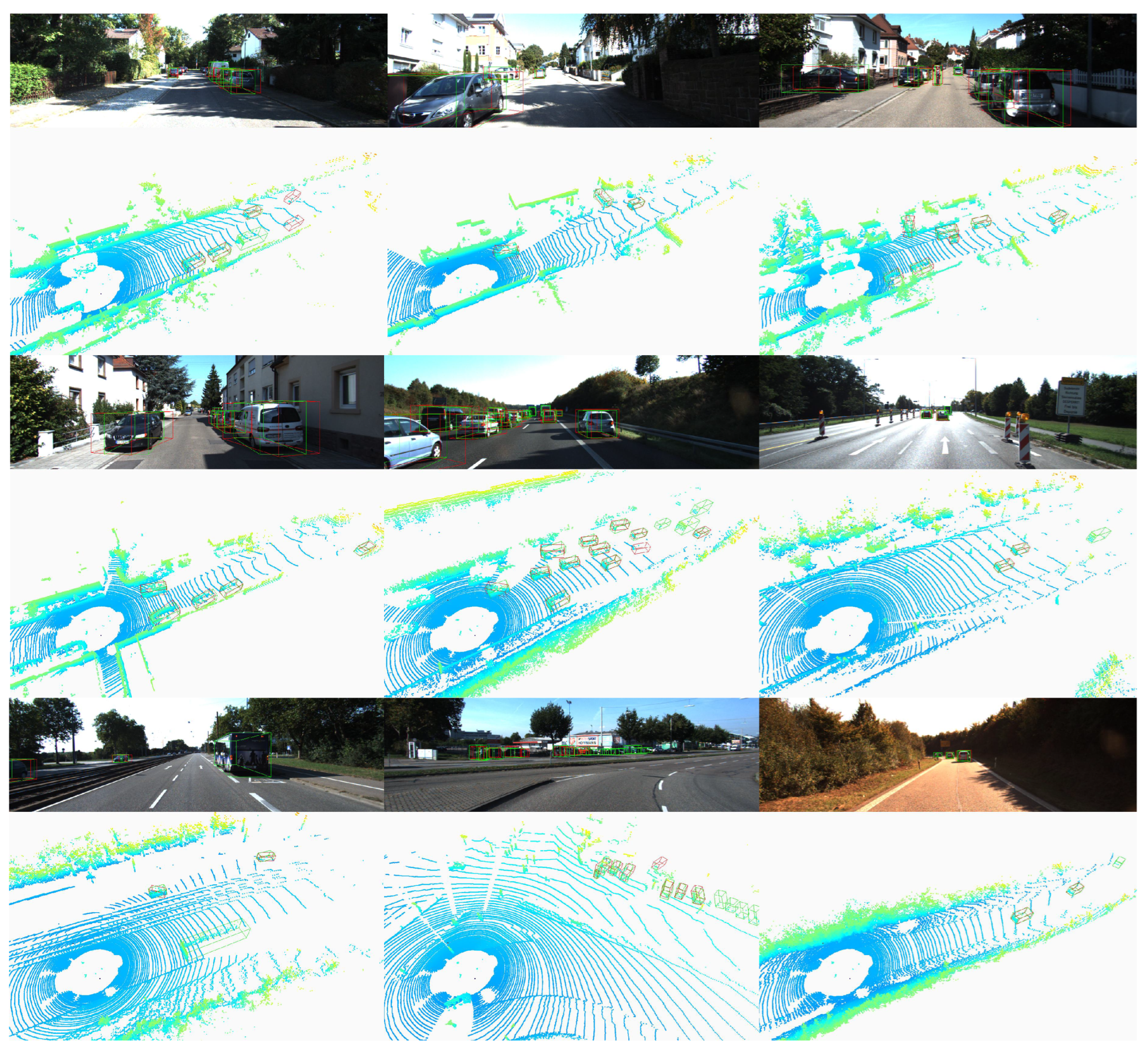
Figure 4 shows the visualization results of the KITTI dataset. The visualization results on the KITTI dataset vividly demonstrate the effectiveness of our method, particularly in detecting small objects at a distance. In the first and third rows of the figure, our method successfully detects vehicles at a significant distance from the sensor. These distant vehicles, appearing small in the point cloud, are accurately identified and enclosed within green bounding boxes. This indicates that our approach can effectively capture and recognize the sparse and subtle point clusters representative of small, distant objects. The successful detection of these distant vehicles underscores the robustness and sensitivity of our method in handling challenging scenarios involving small objects. This capability is crucial for enhancing the safety and reliability of autonomous driving systems, as it ensures that even objects far away from the vehicle can be promptly and accurately detected.
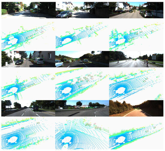
Figure 4.
Extra qualitative results achieved by our method on the validation set of the KITTI dataset. We also show the corresponding projected 3D bounding boxes on images. The Red boxes indicate detected bounding boxes, and green boxes denote ground truth annotations.
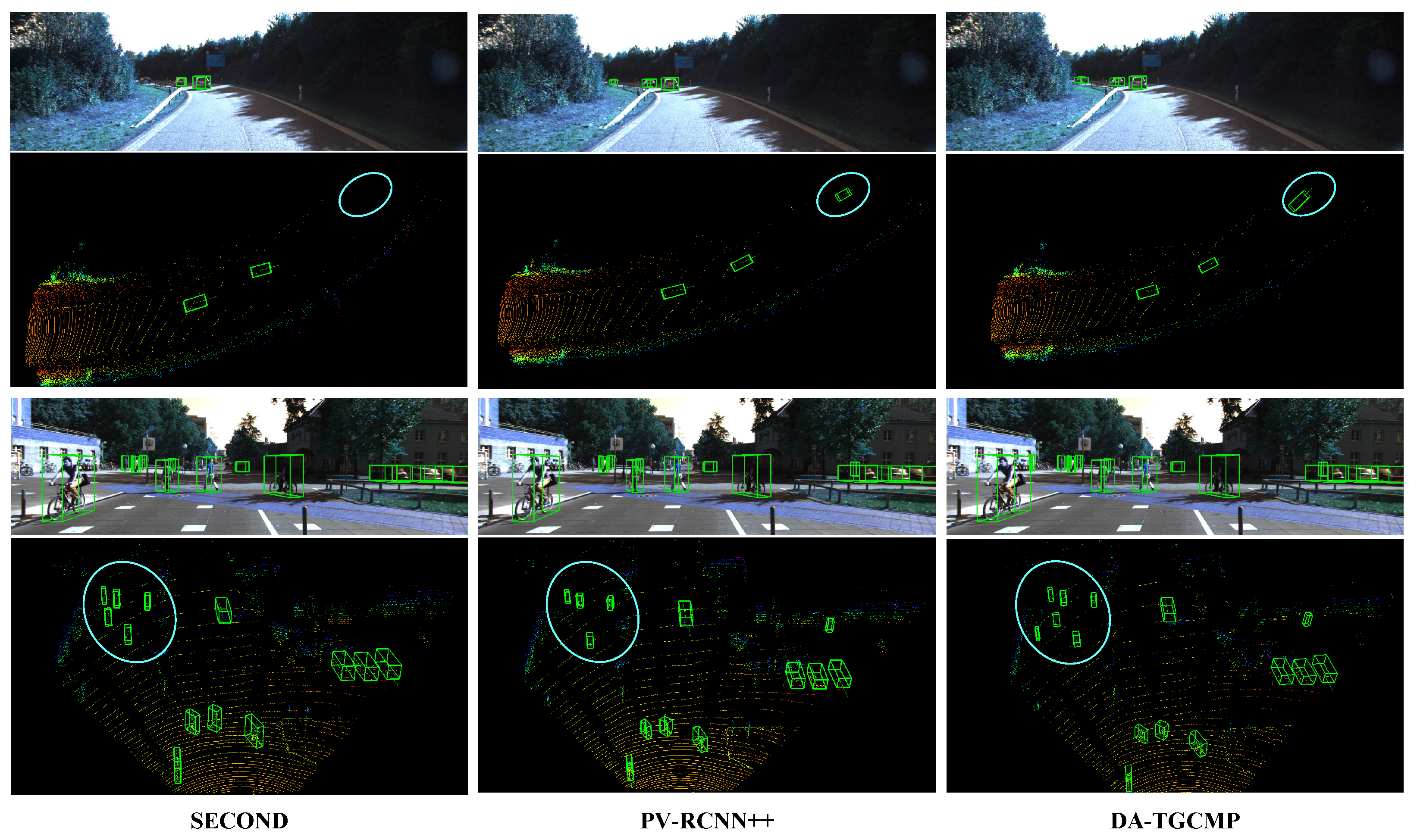
We compare voxel-based SECOND, point-voxel fusion PV-RCNN++, and our DA-TGCMP on highway and urban scenes, as shown in the Figure 5. In highway scenes, SECOND struggles with distant small vehicles, showing missed detections and inaccurate boxes. PV-RCNN++ improves this slightly, but localization remains suboptimal. DA-TGCMP delivers the precise and complete detection of small distant objects, benefiting from the tree–graph cross-message passing that enhances features in sparse regions. In urban scenes, SECOND misses many small objects (e.g., cyclists, pedestrians). PV-RCNN++ detects more objects but suffers from overlap and inaccuracy. DA-TGCMP achieves the accurate and comprehensive detection of small objects by effectively capturing fine-grained features and context. These results highlight that DA-TGCMP significantly improves small-object detection without sacrificing large-object performance.
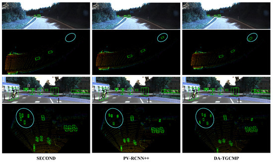
Figure 5.
Qualitative comparison of 3D object detection results on highway and urban scenes. Blue circles highlight small or distant objects. Compared to SECOND and PV-RCNN++, our DA-TGCMP detects more small objects with more accurate and tighter bounding boxes. The blue circles highlight critical regions for comparative analysis.
7. Discussion
The DA-TGCMP framework shows more pronounced improvements in detecting cars compared to pedestrians and cyclists due to the larger size and higher density of point clouds for cars, which allows for more effective feature extraction and modeling. In contrast, the smaller size and sparsity of point clouds for pedestrians and cyclists, along with their more complex and variable shapes, make it harder to achieve the same level of accuracy.
There is a clear trade-off between accuracy and computational efficiency. The TGCMP mechanism, which provides the highest accuracy by enabling bidirectional feature interaction between tree and graph structures, requires the most memory and computational resources. On the other hand, simpler modules like DAGC and HTR offer lower accuracy but are more computationally efficient, making them suitable for resource-constrained settings.
The method is expected to perform well in scenarios with dense point clouds, structured environments, and clear, unoccluded scenes, where both local and global features can be effectively captured. However, it may struggle in situations with sparse point clouds, complex and variable object shapes, and significant occlusion, which can limit the framework’s ability to extract robust features for accurate detection.
Although DA-TGCMP demonstrates strong performance in detecting large objects such as vehicles, challenges remain for small objects like pedestrians and cyclists due to sparse point clouds and complex, variable shapes. In future work, we aim to enhance small-object detection by designing lighter and more efficient feature interaction modules that better capture fine-grained details in sparse and cluttered scenes. We also plan to improve the computational efficiency of the TGCMP mechanism to achieve a better balance between accuracy and real-time performance.
In addition, we intend to extend our framework for the automatic annotation of unlabeled datasets. By leveraging the high accuracy and strong generalization of DA-TGCMP in structured and dense environments, we aim to enable large-scale 3D dataset construction with reduced reliance on manual labeling.
8. Conclusions
In this paper, we present DA-TGCMP, a unified framework that integrates density-aware graphs and hierarchical trees via a novel tree–graph cross-message-passing mechanism. This design bridges the gap between local geometric precision and global contextual understanding, enabling more expressive and robust feature learning for LiDAR-based 3D object detection. Through extensive experiments on three large-scale benchmarks—KITTI, nuScenes, and Waymo—we demonstrate the effectiveness and generalizability of our approach across diverse driving scenarios. Moreover, comprehensive ablation studies confirm the individual contributions of the density-aware graph construction, hierarchical tree representation, and cross-message-passing module, each playing a vital role in boosting detection accuracy. Together, these components make DA-TGCMP a promising solution for advancing 3D perception in autonomous driving systems.
Author Contributions
Methodology, W.Z. and Y.L.; Validation, J.L.; Formal analysis, H.H.; Investigation, H.R.; Writing—original draft, J.Z.; Supervision, H.H. All authors have read and agreed to the published version of the manuscript.
Funding
This research was funded by the Southern Marine Science and Engineering Guangdong Laboratory (Zhuhai) under Grant SML2021SP406.
Data Availability Statement
The original contributions presented in the study are included in the article, further inquiries can be directed to the corresponding author.
Conflicts of Interest
The authors declare no conflict of interest.
References
- Wu, T.J.; He, R.; Peng, C.C. Real-Time Environmental Contour Construction Using 3D LiDAR and Image Recognition with Object Removal. Remote Sens. 2024, 16, 4513. [Google Scholar] [CrossRef]
- Ren, H.; Zhou, R.; Zou, L.; Tang, H. Hierarchical Distribution-Based Exemplar Replay for Incremental SAR Automatic Target Recognition. IEEE Trans. Aerosp. Electron. Syst. 2025, 61, 6576–6588. [Google Scholar] [CrossRef]
- Zhang, X.; Zhang, S.; Sun, Z.; Liu, C.; Sun, Y.; Ji, K.; Kuang, G. Cross-sensor SAR image target detection based on dynamic feature discrimination and center-aware calibration. IEEE Trans. Geosci. Remote Sens. 2025, 63, 5209417. [Google Scholar] [CrossRef]
- Xia, X.; Meng, Z.; Han, X.; Li, H.; Tsukiji, T.; Xu, R.; Zhang, Z.; Ma, J. Automated driving systems data acquisition and processing platform. arXiv 2022, arXiv:2211.13425. [Google Scholar]
- Liao, Z.; Dong, X.; He, Q. Calculating the Optimal Point Cloud Density for Airborne LiDAR Landslide Investigation: An Adaptive Approach. Remote Sens. 2024, 16, 4563. [Google Scholar] [CrossRef]
- Guo, Y.; Wang, H.; Hu, Q.; Liu, H.; Liu, L.; Bennamoun, M. Deep learning for 3d point clouds: A survey. IEEE Trans. Pattern Anal. Mach. Intell. 2020, 43, 4338–4364. [Google Scholar] [CrossRef]
- Gupta, A.; Jain, S.; Choudhary, P.; Parida, M. Dynamic object detection using sparse LiDAR data for autonomous machine driving and road safety applications. Expert Syst. Appl. 2024, 255, 124636. [Google Scholar]
- Li, Y.; Ren, H.; Yu, X.; Zhang, C.; Zou, L.; Zhou, Y. Threshold-free open-set learning network for SAR automatic target recognition. IEEE Sens. J. 2024, 24, 6700–6708. [Google Scholar] [CrossRef]
- Shi, W.; Rajkumar, R. Point-gnn: Graph neural network for 3d object detection in a point cloud. In Proceedings of the IEEE/CVF Conference on Computer Vision and Pattern Recognition, Seattle, WA, USA, 13–19 June 2020; pp. 1711–1719. [Google Scholar]
- Zhang, Y.; Huang, D.; Wang, Y. PC-RGNN: Point cloud completion and graph neural network for 3D object detection. In Proceedings of the AAAI Conference on Artificial Intelligence, Virtually, 2–9 February 2021; Volume 35, pp. 3430–3437. [Google Scholar]
- Yin, J.; Shen, J.; Gao, X.; Crandall, D.J.; Yang, R. Graph neural network and spatiotemporal transformer attention for 3D video object detection from point clouds. IEEE Trans. Pattern Anal. Mach. Intell. 2021, 45, 9822–9835. [Google Scholar] [CrossRef]
- Yue, C.; Wang, Y.; Tang, X.; Chen, Q. DRGCNN: Dynamic region graph convolutional neural network for point clouds. Expert Syst. Appl. 2022, 205, 117663. [Google Scholar] [CrossRef]
- Zhang, R.; Wang, L.; Guo, Z.; Shi, J. Nearest neighbors meet deep neural networks for point cloud analysis. In Proceedings of the IEEE/CVF Winter Conference on Applications of Computer Vision, Waikoloa, HI, USA, 2–7 January 2023; pp. 1246–1255. [Google Scholar]
- Pei, Y.; Zhao, X.; Li, H.; Ma, J.; Zhang, J.; Pu, S. Clusterformer: Cluster-based transformer for 3d object detection in point clouds. In Proceedings of the IEEE/CVF International Conference on Computer Vision, Paris, France, 2–3 October 2023; pp. 6664–6673. [Google Scholar]
- Zhang, M.; Ma, Y.; Li, J.; Zhang, J. A density connection weight-based clustering approach for dataset with density-sparse region. Expert Syst. Appl. 2023, 230, 120633. [Google Scholar] [CrossRef]
- Chen, G.; Wang, M.; Yang, Y.; Yuan, L.; Yue, Y. Fast and Robust Point Cloud Registration with Tree-based Transformer. In Proceedings of the 2024 IEEE International Conference on Robotics and Automation (ICRA), Yokohama, Japan, 13–17 May 2024; pp. 773–780. [Google Scholar]
- Pang, J.; Bui, K.; Tian, D. PIVOT-Net: Heterogeneous point-voxel-tree-based framework for point cloud compression. In Proceedings of the 2024 International Conference on 3D Vision (3DV), Davos, Switzerland, 18–21 March 2024; pp. 1270–1279. [Google Scholar]
- Ren, S.; Pan, X.; Zhao, W.; Nie, B.; Han, B. Dynamic graph transformer for 3D object detection. Knowl.-Based Syst. 2023, 259, 110085. [Google Scholar] [CrossRef]
- Vonessen, C.; Grötschla, F.; Wattenhofer, R. Next Level Message-Passing with Hierarchical Support Graphs. arXiv 2024, arXiv:2406.15852. [Google Scholar]
- Zhou, Y.; Tuzel, O. Voxelnet: End-to-end learning for point cloud based 3d object detection. In Proceedings of the IEEE Conference on Computer Vision and Pattern Recognition, Salt Lake City, UT, USA, 18–22 June 2018; pp. 4490–4499. [Google Scholar]
- Yan, Y.; Mao, Y.; Li, B. Second: Sparsely embedded convolutional detection. Sensors 2018, 18, 3337. [Google Scholar] [CrossRef]
- Lang, A.H.; Vora, S.; Caesar, H.; Zhou, L.; Yang, J.; Beijbom, O. Pointpillars: Fast encoders for object detection from point clouds. In Proceedings of the IEEE/CVF Conference on Computer Vision and Pattern Recognition, Long Beach, CA, USA, 15–20 June 2019; pp. 12697–12705. [Google Scholar]
- Shi, S.; Wang, Z.; Shi, J.; Wang, X.; Li, H. From points to parts: 3d object detection from point cloud with part-aware and part-aggregation network. IEEE Trans. Pattern Anal. Mach. Intell. 2020, 43, 2647–2664. [Google Scholar] [CrossRef]
- Deng, J.; Shi, S.; Li, P.; Zhou, W.; Zhang, Y.; Li, H. Voxel r-cnn: Towards high performance voxel-based 3d object detection. In Proceedings of the AAAI Conference on Artificial Intelligence, Virtually, 2–9 February 2021; Volume 35, pp. 1201–1209. [Google Scholar]
- Ye, M.; Xu, S.; Cao, T. Hvnet: Hybrid voxel network for lidar based 3d object detection. In Proceedings of the IEEE/CVF Conference on Computer Vision and Pattern Recognition, Seattle, WA, USA, 14–19 June 2020; pp. 1631–1640. [Google Scholar]
- Zheng, W.; Tang, W.; Chen, S.; Jiang, L.; Fu, C.W. Cia-ssd: Confident iou-aware single-stage object detector from point cloud. In Proceedings of the AAAI Conference on Artificial Intelligence, Virtually, 19–21 May 2021; Volume 35, pp. 3555–3562. [Google Scholar]
- Mao, J.; Xue, Y.; Niu, M.; Bai, H.; Feng, J.; Liang, X.; Xu, H.; Xu, C. Voxel transformer for 3d object detection. In Proceedings of the IEEE/CVF International Conference on Computer Vision, Virtually, 2–9 February 2021; pp. 3164–3173. [Google Scholar]
- Yang, Y.Q.; Guo, Y.X.; Xiong, J.Y.; Liu, Y.; Pan, H.; Wang, P.S.; Tong, X.; Guo, B. Swin3d: A pretrained transformer backbone for 3d indoor scene understanding. Comput. Vis. Media 2025, 11, 83–101. [Google Scholar] [CrossRef]
- Shi, S.; Wang, X.; Li, H. Pointrcnn: 3d object proposal generation and detection from point cloud. In Proceedings of the IEEE/CVF Conference on Computer Vision and Pattern Recognition, Long Beach, CA, USA, 15–20 June 2019; pp. 770–779. [Google Scholar]
- Qi, C.R.; Yi, L.; Su, H.; Guibas, L.J. Pointnet++: Deep hierarchical feature learning on point sets in a metric space. Adv. Neural Inf. Process. Syst. 2017, 30, 5105–5114. [Google Scholar]
- Yang, Z.; Sun, Y.; Liu, S.; Jia, J. 3dssd: Point-based 3d single stage object detector. In Proceedings of the IEEE/CVF Conference on Computer Vision and Pattern Recognition, Seattle, WA, USA, 14–19 June 2020; pp. 11040–11048. [Google Scholar]
- Zhang, Y.; Hu, Q.; Xu, G.; Ma, Y.; Wan, J.; Guo, Y. Not all points are equal: Learning highly efficient point-based detectors for 3d lidar point clouds. In Proceedings of the IEEE/CVF Conference on Computer Vision and Pattern Recognition, New Orleans, LA, USA, 18–24 June 2022; pp. 18953–18962. [Google Scholar]
- Yang, Z.; Sun, Y.; Liu, S.; Shen, X.; Jia, J. STD: Sparse-to-Dense 3D Object Detector for Point Cloud. In Proceedings of the 2019 IEEE/CVF International Conference on Computer Vision (ICCV), Seoul, Republic of Korea, 27 October–2 November 2019; pp. 1951–1960. [Google Scholar] [CrossRef]
- He, C.; Zeng, H.; Huang, J.; Hua, X.S.; Zhang, L. Structure aware single-stage 3d object detection from point cloud. In Proceedings of the IEEE/CVF Conference on Computer Vision and Pattern Recognition, Seattle, WA, USA, 14–19 June 2020; pp. 11873–11882. [Google Scholar]
- Shi, S.; Guo, C.; Jiang, L.; Wang, Z.; Shi, J.; Wang, X.; Li, H. Pv-rcnn: Point-voxel feature set abstraction for 3d object detection. In Proceedings of the IEEE/CVF Conference on Computer Vision and Pattern Recognition, Seattle, WA, USA, 14–19 June 2020; pp. 10529–10538. [Google Scholar]
- Sheng, H.; Cai, S.; Liu, Y.; Deng, B.; Huang, J.; Hua, X.S.; Zhao, M.J. Improving 3d object detection with channel-wise transformer. In Proceedings of the IEEE/CVF International Conference on Computer Vision, Montreal, BC, Canada, 11–17 October 2021; pp. 2743–2752. [Google Scholar]
- Mao, J.; Niu, M.; Bai, H.; Liang, X.; Xu, H.; Xu, C. Pyramid r-cnn: Towards better performance and adaptability for 3d object detection. In Proceedings of the IEEE/CVF International Conference on Computer Vision, Montreal, BC, Canada, 11–17 October 2021; pp. 2723–2732. [Google Scholar]
- Li, Y.; Ma, L.; Tan, W.; Sun, C.; Cao, D.; Li, J. GRNet: Geometric relation network for 3D object detection from point clouds. ISPRS J. Photogramm. Remote Sens. 2020, 165, 43–53. [Google Scholar] [CrossRef]
- Chen, J.; Lei, B.; Song, Q.; Ying, H.; Chen, D.Z.; Wu, J. A hierarchical graph network for 3d object detection on point clouds. In Proceedings of the IEEE/CVF Conference on Computer Vision and Pattern Recognition, Seattle, WA, USA, 14–19 June 2020; pp. 392–401. [Google Scholar]
- Cheng, H.; Zhu, J.; Lu, J.; Han, X. EDGCNet: Joint dynamic hyperbolic graph convolution and dual squeeze-and-attention for 3D point cloud segmentation. Expert Syst. Appl. 2024, 237, 121551. [Google Scholar] [CrossRef]
- He, Q.; Wang, Z.; Zeng, H.; Zeng, Y.; Liu, Y. Svga-net: Sparse voxel-graph attention network for 3d object detection from point clouds. In Proceedings of the AAAI Conference on Artificial Intelligence, Online, 22 February–1 March 2022; Volume 36, pp. 870–878. [Google Scholar]
- Sun, Z.; Leng, X.; Zhang, X.; Zhou, Z.; Xiong, B.; Ji, K.; Kuang, G. Arbitrary-direction SAR ship detection method for multi-scale imbalance. IEEE Trans. Geosci. Remote Sens. 2025, 63, 5208921. [Google Scholar] [CrossRef]
- Wang, R.; Wang, Z.; Zhang, G.; Kang, H.; Luo, F. KD-Net: A novel knowledge-and data-driven network for SAR target recognition with limited data. In Proceedings of the IET International Radar Conference (IRC 2023), IET, Chongqing, China, 3–5 December 2023; Volume 2023, pp. 2623–2627. [Google Scholar]
- Han, K.; Xiao, A.; Wu, E.; Guo, J.; Xu, C.; Wang, Y. Transformer in transformer. Adv. Neural Inf. Process. Syst. 2021, 34, 15908–15919. [Google Scholar]
- Dosovitskiy, A.; Beyer, L.; Kolesnikov, A.; Weissenborn, D.; Zhai, X.; Unterthiner, T.; Dehghani, M.; Minderer, M.; Heigold, G.; Gelly, S.; et al. An image is worth 16x16 words: Transformers for image recognition at scale. arXiv 2020, arXiv:2010.11929. [Google Scholar]
- Zhou, W.; Jiang, W.; Zheng, Z.; Li, J.; Su, T.; Hu, H. From grids to pseudo-regions: Dynamic memory augmented image captioning with dual relation transformer. Expert Syst. Appl. 2025, 273, 126850. [Google Scholar] [CrossRef]
- Carion, N.; Massa, F.; Synnaeve, G.; Usunier, N.; Kirillov, A.; Zagoruyko, S. End-to-end object detection with transformers. In Proceedings of the European Conference on Computer Vision, Glasgow, UK, 23–28 August 2020; Springer: Berlin/Heidelberg, Germany, 2020; pp. 213–229. [Google Scholar]
- Liu, Z.; Lin, Y.; Cao, Y.; Hu, H.; Wei, Y.; Zhang, Z.; Lin, S.; Guo, B. Swin transformer: Hierarchical vision transformer using shifted windows. In Proceedings of the IEEE/CVF International Conference on Computer Vision, Montreal, BC, Canada, 11–17 October 2021; pp. 10012–10022. [Google Scholar]
- Yu, X.; Tang, L.; Rao, Y.; Huang, T.; Zhou, J.; Lu, J. Point-bert: Pre-training 3d point cloud transformers with masked point modeling. In Proceedings of the IEEE/CVF Conference on Computer Vision and Pattern Recognition, New Orleans, LA, USA, 18–24 June 2022; pp. 19313–19322. [Google Scholar]
- Pan, X.; Xia, Z.; Song, S.; Li, L.E.; Huang, G. 3d object detection with pointformer. In Proceedings of the IEEE/CVF Conference on Computer Vision and Pattern Recognition, Nashville, TN, USA, 19–25 June 2021; pp. 7463–7472. [Google Scholar]
- Ning, Y.; Cao, J.; Bao, C.; Hao, Q. DVST: Deformable voxel set transformer for 3D object detection from point clouds. Remote Sens. 2023, 15, 5612. [Google Scholar] [CrossRef]
- Xu, X.; Dong, S.; Xu, T.; Ding, L.; Wang, J.; Jiang, P.; Song, L.; Li, J. Fusionrcnn: Lidar-camera fusion for two-stage 3d object detection. Remote Sens. 2023, 15, 1839. [Google Scholar] [CrossRef]
- Chen, Z.; Pham, K.T.; Ye, M.; Shen, Z.; Chen, Q. Cross-Cluster Shifting for Efficient and Effective 3D Object Detection in Autonomous Driving. In Proceedings of the 2024 IEEE International Conference on Robotics and Automation (ICRA), Yokohama, Japan, 13–17 May 2024; pp. 4273–4280. [Google Scholar]
- Lin, T.Y.; Goyal, P.; Girshick, R.; He, K.; Dollár, P. Focal loss for dense object detection. In Proceedings of the IEEE International Conference on Computer Vision, Venice, Italy, 22–29 October 2017; pp. 2980–2988. [Google Scholar]
- Shi, S.; Jiang, L.; Deng, J.; Wang, Z.; Guo, C.; Shi, J.; Wang, X.; Li, H. PV-RCNN++: Point-voxel feature set abstraction with local vector representation for 3D object detection. Int. J. Comput. Vis. 2023, 131, 531–551. [Google Scholar] [CrossRef]
- Kingma, D.P.; Ba, J. Adam: A method for stochastic optimization. arXiv 2014, arXiv:1412.6980. [Google Scholar]
- Qi, C.R.; Liu, W.; Wu, C.; Su, H.; Guibas, L.J. Frustum pointnets for 3d object detection from rgb-d data. In Proceedings of the IEEE Conference on Computer Vision and Pattern Recognition, Salt Lake City, UT, USA, 18–22 June 2018; pp. 918–927. [Google Scholar]
- Vora, S.; Lang, A.H.; Helou, B.; Beijbom, O. Pointpainting: Sequential fusion for 3d object detection. In Proceedings of the IEEE/CVF Conference on Computer Vision and Pattern Recognition, Seattle, WA, USA, 14–19 June2020; pp. 4604–4612. [Google Scholar]
- Yoo, J.H.; Kim, Y.; Kim, J.; Choi, J.W. 3d-cvf: Generating joint camera and lidar features using cross-view spatial feature fusion for 3d object detection. In Proceedings of the Computer Vision–ECCV 2020: 16th European Conference, Glasgow, UK, 23–28 August 2020; Proceedings, Part XXVII 16. Springer: Berlin/Heidelberg, Germany, 2020; pp. 720–736. [Google Scholar]
- Xie, T.; Wang, L.; Wang, K.; Li, R.; Zhang, X.; Zhang, H.; Yang, L.; Liu, H.; Li, J. FARP-Net: Local-global feature aggregation and relation-aware proposals for 3D object detection. IEEE Trans. Multimed. 2023, 26, 1027–1040. [Google Scholar] [CrossRef]
- Yang, H.; Wang, W.; Chen, M.; Lin, B.; He, T.; Chen, H.; He, X.; Ouyang, W. Pvt-ssd: Single-stage 3d object detector with point-voxel transformer. In Proceedings of the IEEE/CVF Conference on Computer Vision and Pattern Recognition, Vancouver, BC, Canada, 18–22 June 2023; pp. 13476–13487. [Google Scholar]
- Noh, J.; Lee, S.; Ham, B. Hvpr: Hybrid voxel-point representation for single-stage 3d object detection. In Proceedings of the IEEE/CVF Conference on Computer Vision and Pattern Recognition, Nashville, TN, USA, 19–25 June 2021; pp. 14605–14614. [Google Scholar]
- Wang, C.H.; Chen, H.W.; Chen, Y.; Hsiao, P.Y.; Fu, L.C. VoPiFNet: Voxel-pixel fusion network for multi-class 3D object detection. IEEE Trans. Intell. Transp. Syst. 2024, 25, 8527–8537. [Google Scholar] [CrossRef]
- Yin, T.; Zhou, X.; Krähenbühl, P. Multimodal virtual point 3d detection. Adv. Neural Inf. Process. Syst. 2021, 34, 16494–16507. [Google Scholar]
- Xu, S.; Zhou, D.; Fang, J.; Yin, J.; Bin, Z.; Zhang, L. Fusionpainting: Multimodal fusion with adaptive attention for 3d object detection. In Proceedings of the 2021 IEEE International Intelligent Transportation Systems Conference (ITSC), Indianapolis, IN, USA, 19–22 September 2021; pp. 3047–3054. [Google Scholar]
- Nagesh, S.; Baig, A.; Srinivasan, S.; Rangesh, A.; Trivedi, M. Structure Aware and Class Balanced 3D Object Detection on nuScenes Dataset. arXiv 2022, arXiv:2205.12519. [Google Scholar]
- Chen, Y.; Liu, J.; Zhang, X.; Qi, X.; Jia, J. Largekernel3d: Scaling up kernels in 3d sparse cnns. In Proceedings of the IEEE/CVF Conference on Computer Vision and Pattern Recognition, Vancouver, BC, Canada, 18–22 June2023; pp. 13488–13498. [Google Scholar]
- Bai, X.; Hu, Z.; Zhu, X.; Huang, Q.; Chen, Y.; Fu, H.; Tai, C.L. Transfusion: Robust lidar-camera fusion for 3d object detection with transformers. In Proceedings of the IEEE/CVF Conference on Computer Vision and Pattern Recognition, New Orleans, LA, USA, 18–24 June 2022; pp. 1090–1099. [Google Scholar]
- Shi, G.; Li, R.; Ma, C. Pillarnet: Real-time and high-performance pillar-based 3d object detection. In Proceedings of the European Conference on Computer Vision, Milan, Italy, 23–27 October 2022; Springer: Berlin/Heidelberg, Germany, 2022; pp. 35–52. [Google Scholar]
- Zhou, Y.; Sun, P.; Zhang, Y.; Anguelov, D.; Gao, J.; Ouyang, T.; Guo, J.; Ngiam, J.; Vasudevan, V. End-to-end multi-view fusion for 3d object detection in lidar point clouds. In Proceedings of the Conference on Robot Learning, PMLR, Virtual, 16–18 November 2020; pp. 923–932. [Google Scholar]
- Ge, R.; Ding, Z.; Hu, Y.; Wang, Y.; Chen, S.; Huang, L.; Li, Y. Afdet: Anchor free one stage 3d object detection. arXiv 2020, arXiv:2006.12671. [Google Scholar]
- Wang, Y.; Fathi, A.; Kundu, A.; Ross, D.A.; Pantofaru, C.; Funkhouser, T.; Solomon, J. Pillar-based object detection for autonomous driving. In Proceedings of the European Conference on Computer Vision, Glasgow, UK, 23–28 August 2020; Springer: Berlin/Heidelberg, Germany, 2020; pp. 18–34. [Google Scholar]
- Yin, T.; Zhou, X.; Krahenbuhl, P. Center-based 3d object detection and tracking. In Proceedings of the IEEE/CVF Conference on Computer Vision and Pattern Recognition, Nashville, TN, USA, 19–25 June 2021; pp. 11784–11793. [Google Scholar]
- Zhu, Z.; Meng, Q.; Wang, X.; Wang, K.; Yan, L.; Yang, J. Curricular object manipulation in lidar-based object detection. In Proceedings of the IEEE/CVF Conference on Computer Vision and Pattern Recognition, Vancouver, BC, Canada, 18–22 June 2023; pp. 1125–1135. [Google Scholar]
- Nie, M.; Xue, Y.; Wang, C.; Ye, C.; Xu, H.; Zhu, X.; Huang, Q.; Mi, M.B.; Wang, X.; Zhang, L. Partner: Level up the polar representation for lidar 3d object detection. In Proceedings of the IEEE/CVF International Conference on Computer Vision, Paris, France, 2–3 October 2023; pp. 3801–3813. [Google Scholar]
- Lu, B.; Sun, Y.; Yang, Z. Voxel graph attention for 3-D object detection from point clouds. IEEE Trans. Instrum. Meas. 2023, 72, 5023012. [Google Scholar] [CrossRef]

Disclaimer/Publisher’s Note: The statements, opinions and data contained in all publications are solely those of the individual author(s) and contributor(s) and not of MDPI and/or the editor(s). MDPI and/or the editor(s) disclaim responsibility for any injury to people or property resulting from any ideas, methods, instructions or products referred to in the content. |
© 2025 by the authors. Licensee MDPI, Basel, Switzerland. This article is an open access article distributed under the terms and conditions of the Creative Commons Attribution (CC BY) license (https://creativecommons.org/licenses/by/4.0/).