Utilization of Multisensor Satellite Data for Developing Spatial Distribution of Methane Emission on Rice Paddy Field in Subang, West Java

Abstract

Intergovernmental Panel on Climate Change (IPCC) guidelines have been standardized and widely used to calculate methane (CH₄) emissions from paddy fields. The emission factor (EF) is a key parameter in these guidelines, and it is different for each location globally and regionally. However, limited studies have been conducted to measure locally specific EFs (EFlocal) through on-site assessments and modeling their spatial distribution effectively. This study aims to investigate the potential of multisensor satellite data to develop a spatial model of CH₄ emission estimation on rice paddy fields under different water management practices, i.e., continuous flooding (CF) and alternate wetting and drying (AWD) in Subang, West Java, Indonesia. The model employed the national EF (EFnational) and EFlocal using the IPCC guidelines. In this study, we employed the multisensor satellite data to derive the key parameters for estimating CH₄ emission, i.e., rice cultivation area, rice age, and EF. Optical high-resolution images were used to delineate the rice cultivation area, Sentinel-1 SAR imagery was used for identifying transplanting and harvesting dates for rice age estimation, and ALOS-2/PALSAR-2 was used to map the water regime for determining the scaling factor of the EF. The closed-chamber method has been used to measure the daily CH₄ flux rate on the local sites. The results revealed spatial variability in CH₄ emissions, ranging from 1–5 kg/crop/season to 20–30 kg/crop/season, depending on the water regime. Fields under CF exhibited higher CH₄ emissions than those under AWD, underscoring the critical role of water management in mitigating CH₄ emissions. This study demonstrates the feasibility of combining remote sensing data with the IPCC model to spatially estimate CH₄ emissions, providing a robust framework for sustainable rice cultivation and greenhouse gas (GHG) mitigation strategies.

1. Introduction

Methane (CH₄) emissions from rice paddies are a significant source of greenhouse gases, accounting for approximately 10% of global agricultural emissions [1,2]. Methane production in paddy fields occurs under anaerobic conditions, particularly in continuously flooded fields, which create an ideal environment for methanogenic bacteria [3]. As a staple food for over half of the world’s population, sustainable rice cultivation is crucial for balancing food security and climate mitigation [4].

Several models exist to quantify greenhouse gas emissions from agriculture. For instance, the National Emission Model for Agriculture (NEMA) was developed to calculate gas emissions from different categories of agricultural activities, including grazing, animal housing, fertilizer use, manure storage, and crop cultivation [5]. However, it relies on the Total Ammoniacal Nitrogen (TAN) flow data for every category, and such data may not be fully available in the local scope. Another method, life cycle assessment (LCA), offers a comprehensive insight into environmental impact by considering all stages in the agricultural activities but demands a large amount of data and resources for accurate assessments [6].

The Intergovernmental Panel on Climate Change (IPCC) guidelines provide a standardized methodology for estimating CH₄ emissions from agricultural sources. A critical parameter in these calculations is the emission factor (EF), which varies based on water regime, soil characteristics, and farming practices. The IPCC provides a tiered approach to address different data availability and accuracy levels: Tier 1, Tier 2, and Tier 3 [2]. Tier 1 uses default global emission factors provided by the IPCC. Meanwhile, Tier 2 uses country-specific emission factors (EFnational), which offer improved accuracy but still fail to capture local field variations [7,8]. Tier 3 provides detailed models and high-resolution data. It often integrates remote sensing and advanced simulation models to capture local field variations, particularly in agricultural systems with varying water management and land use practices. A problem of the EFnational is its inability to capture local field variations accurately, further highlighting the necessity of locally specific emission factors (EFlocal) for more precise estimations.

Accurate estimation of CH₄ emissions from rice paddies remains challenging due to the spatial heterogeneity of farming systems and environmental conditions [2,7]. Water management practices, such as alternate wetting and drying (AWD) and Continuous Flooding (CF), significantly influence CH₄ emissions but are not uniformly represented in EFnational calculations [2]. Moreover, although closed-chamber methods are effective for on-site CH₄ measurements, they are rarely integrated with spatial modeling approaches [9,10,11]. The limited integration of the EFlocal with spatial modeling highlights a gap in research, creating opportunities for further study in CH₄ emission estimation.

Previous research has predominantly focused on regional-scale CH₄ emission estimates using standardized EF values or local-scale measurements lacking spatial context [7,8,9]. Remote sensing technologies, both optical and synthetic aperture radar (SAR) sensors, offer spatial information on rice paddies to provide spatial CH₄ emission estimation [12,13,14,15]. In general, the space-based rice paddy mapping can be established from four methods, i.e., (1) spatial statistical method, which combines the statistical data of agriculture and satellite data into gridded maps [16]; (2) phenology-based method, which maps flooding, vegetative, and generative stages of rice paddy using Normalized Difference Vegetation Index (NDVI), Enhanced Vegetation Index (EVI), polarized backscatter values, and Land Surface Water Index (LSWI) [17,18,19,20]; and (3) traditional machine learning method, consisting of unsupervised [21] and supervised classification [22,23], and (4) deep learning method [24,25].

Space-based rice paddy products are crucial in mapping the spatial distribution of CH₄ emissions and have been widely explored in many studies across Asia [12,13,14,15,26,27,28,29,30]. For instance, the Mekong Delta, Vietnam, has been studied the potential of ALOS-2 PALSAR-2 for differentiating inundated and non-inundated paddy fields for methane calculations [12]. In Korea, satellite data has been used for methane calculation using IPCC guidelines [13]. Similar efforts have been conducted in China and Thailand to evaluate emission variability under varying water regimes and cultivation practices [14,15].

However, despite growing international interest, research on space-based mapping of CH₄ emissions focusing on Indonesian rice fields remains limited. Under tropical atmospheric conditions, cloud cover often hinders optical satellite observations, making SAR data a valuable alternative for reliable monitoring of rice paddy conditions in Indonesia. C-band SAR is particularly effective in mapping rice phenology [31], while L-band SAR is well-suited for soil moisture detection or water regime mapping [32,33]. Additionally, a gap remains in converting local EF measurements into spatial CH₄ emission models, highlighting the need for a comprehensive approach integrating on-site closed-chamber measurements with remote sensing data to address spatial variability in CH₄ emissions.

This study aims to investigate the potential of multisensor satellite data to develop a spatial model of CH₄ emission estimation on rice paddy fields, using national (EFnational) and local (EFlocal) emission factors based on the IPCC guidelines under AWD and CF practice in paddy cultivation in Subang, West Java, Indonesia. The methodology includes using remote sensing data to delineate rice cultivation areas, assess phenological stages for rice age calculation, and derive water regime scaling factors while incorporating the EFlocal based on closed-chamber method measurements to represent local conditions accurately. This research demonstrates the feasibility of combining remote sensing technologies with the IPCC model to provide spatial CH₄ emission estimates.

2. Materials and Methods

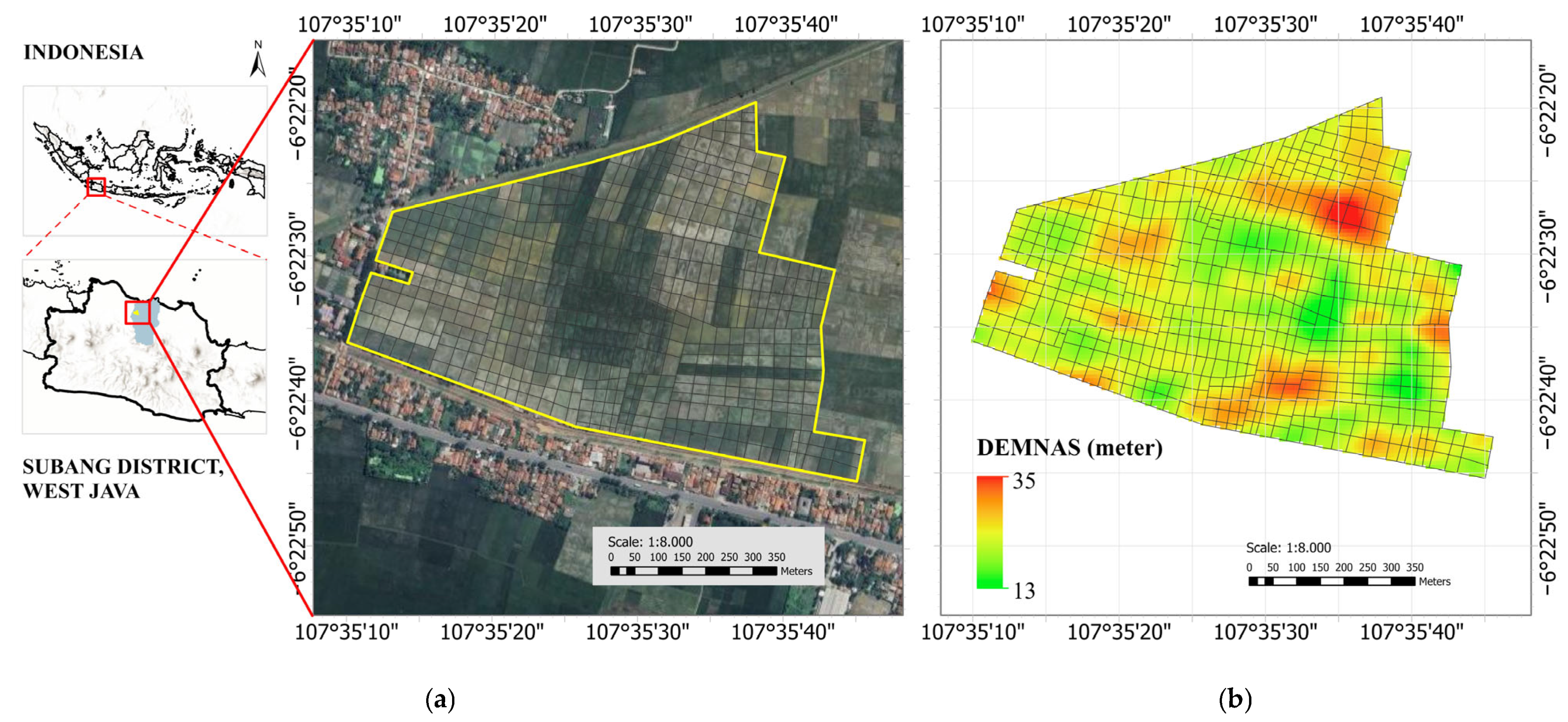
2.1. Study Area

Subang district, located in West Java, is the third-largest rice production area in Indonesia [34]. The study is in the rice fields of Ciberes Village in Subang District, which is known for its well-managed irrigation practice system. The total area of the study location is 50 hectares (ha), with 580 rice field parcels. The study site is bordered by irrigation infrastructure in the north, south, and west. Figure 1 shows the study site.

The area is cultivated with glutinous rice varieties using local AWD practices and conventional CF irrigation methods. It is located at 107°35′10″–107°35′50″ E and 6°22′20″–6°22′50″ S, with elevation ranging from 13 to 35 m above sea level referring to the National Digital Elevation Model (DEMNAS) data. DEMNAS was obtained from the Indonesian Geospatial Information Agency (BIG) with a spatial resolution of approximately 8 m. The central part of the area is at a lower elevation than its surrounding area, causing the rice fields to remain constantly flooded with irrigation water. Chambers and water level devices were installed in the three rice field samples, with two samples representing AWD practices and one sample representing CF practices.

The study area is in the northern part of the Subang District, where the region borders the Java Sea. It is characterized by fluvial landforms shaped by fluvial processes resulting from flowing water, processes, and central and/or surface flow [35]. According to geological maps [36], the area has tuffaceous sandstone and conglomerate formed from sedimentary rock. This region experiences a monsoonal rainfall pattern, so it has high rainfall intensity (reach > 400 mm/month) at the beginning (January–March) and end of the year (November–December), while the lowest is 0 mm/month during the driest period (August–September) [37]. In Subang, rice cultivation follows a biannual cropping system, enabling farmers to achieve two harvests per year. The primary planting season coincides with the rainy season and varies from November to March, whereas the secondary season occurs during the drier months from August to October. Each rice cycle spans around 100 days after transplanting (DAT).

2.2. Data Collection and Pre-Processing

2.2.1. Sentinel-1 for Rice Age Identification

Sentinel-1 C-band synthetic aperture radar (SAR) data used in this study were obtained from the Google Earth Engine (GEE) data catalog (COPERNICUS/S1_GRD image collection), which provides Level-1 Ground Range Detected (GRD) products. The images were pre-processed using the Sentinel-1 Toolbox (S1TBX), following standard procedures, including the application of orbit files, removal of border and thermal noise, radiometric calibration, and terrain correction. This processing produced calibrated, orthorectified backscatter coefficient (σ°) products expressed in decibels (dB). The backscatter coefficient represents the radar cross-section per unit ground area and indicates whether the terrain preferentially scatters the incident microwave signal away from (dB < 0) or toward (dB > 0) the SAR sensor, depending on surface geometry and electromagnetic properties. (https://developers.google.com/earth-engine/guides/sentinel1 (accessed on 2 March 2024)).

In this study, VH-polarized Sentinel-1 images acquired on 1 February and 21 June 2024—covering a complete rice-growing cycle in the study area—were used to estimate rice crop ages by analyzing phenological stages through temporal variations in backscatter response. All images were acquired in ascending orbits. The availability of two overlapping Sentinel-1 scenes reduced the temporal revisit interval to fewer than 12 days.

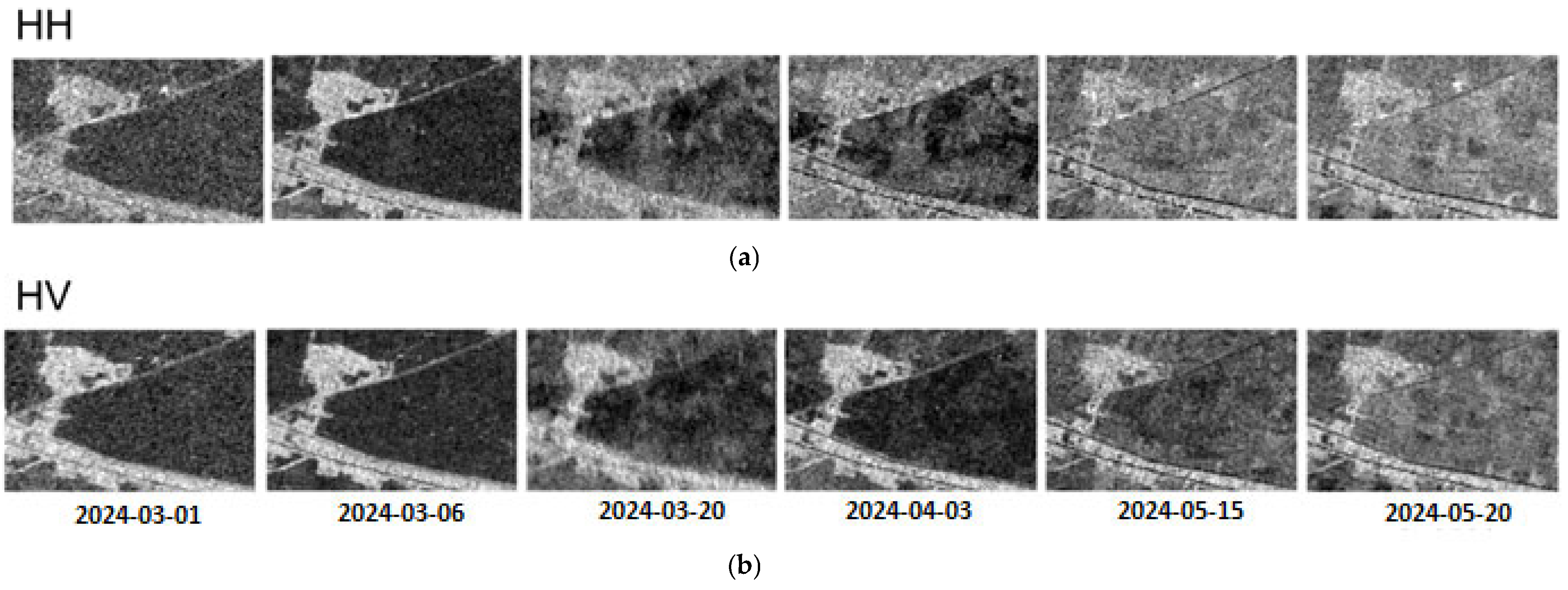
2.2.2. ALOS-2/PALSAR-2 for Water Regime Analysis

The ALOS-2/PALSAR-2 dataset used in this study was provided by the Japan Aerospace Exploration Agency (JAXA) and delivered with a spatial resolution of 10 m. Six images were acquired in Stripmap Fine mode with L2.1 horizontal dual-polarization (HH+HV) between 1 March and 20 May 2024, covering a substantial portion of a single paddy growing season, from transplanting to harvest (Figure 2).

Figure 2 shows the temporal variation in backscatter at the study site over the cropping season. The predominantly dark tones in March 2024 indicate low backscatter values, corresponding to the transplanting stage when fields were largely inundated. As the crop advances through the vegetative and generative phases, backscatter values increase, resulting in progressively lighter tones. By May 2024, the imagery shows a brighter appearance, reflecting the harvest stage, when the water has receded and fields are comparatively dry.

The standard data of ALOS-2/PALSAR-2 level 2.1 from JAXA was converted to backscatter coefficients ($\sigma$/sigma naught) in the decibel (dB) scale [38] following Formula (1).

$${\sigma }_{Q16}^0=10·{log}_{10}〈{DN}^2〉+{CalFac}_1$$

(1)

where ${\sigma }_{Q16}^0$ is the backscatter coefficient, DN is the digital number of each polarization, and CalFac₁ is the calibration factor.

The polarimetric data, specifically the HH and HV polarization, were further transformed into natural backscatter value (NV) to enhance their interpretability. The transformation was computed using Formula (2):

$$\mathrm{NV}=10^{({\sigma }_{Q16}^0/10)}$$

(2)

where NV is the natural backscatter value, and ${\sigma }_{Q16}^0$ is the backscatter coefficient

Speckle noise caused by coherent radar signals’ random constructive and destructive interference degrades image quality and complicates feature interpretation [39]. The Lee filter [40] with a 7 × 7 window size was applied to reduce this speckle noise. The filtered data were then converted back to backscatter coefficients ($\sigma$) in decibel (dB) format using Formula (3):

$$\sigma =10lo{g}_{10}\left(NV\right)$$

(3)

where $\sigma$ is the backscatter coefficient, and NV is the natural backscatter value.

2.2.3. Daily Flux of Local CH₄ from Closed-Chamber

Field data were collected through biweekly CH₄ flux measurements during the rice-growing season under AWD and CF irrigation practices, at approximately 14, 28, 41, 56, 71, and 85 DAT. Measurements were conducted from 7 March 2024 to 17 May 2024. The dataset includes CH₄ concentration values (ppm), which were converted to CH₄ fluxes (kg parcel⁻¹ day⁻¹) using chamber volume, temperature corrections, and the ideal gas law. This conversion is essential for accurately quantifying methane emissions, as it standardizes emissions over specific areas and time periods. Calculating fluxes enables consistent comparisons across irrigation practices and growth stages and also facilitates integration with remote sensing data for spatially explicit emission estimates at larger scales. Further methodological details are provided in Section 2.3.5.

2.2.4. Water Level Measurement Using Internet of Things (IoT)

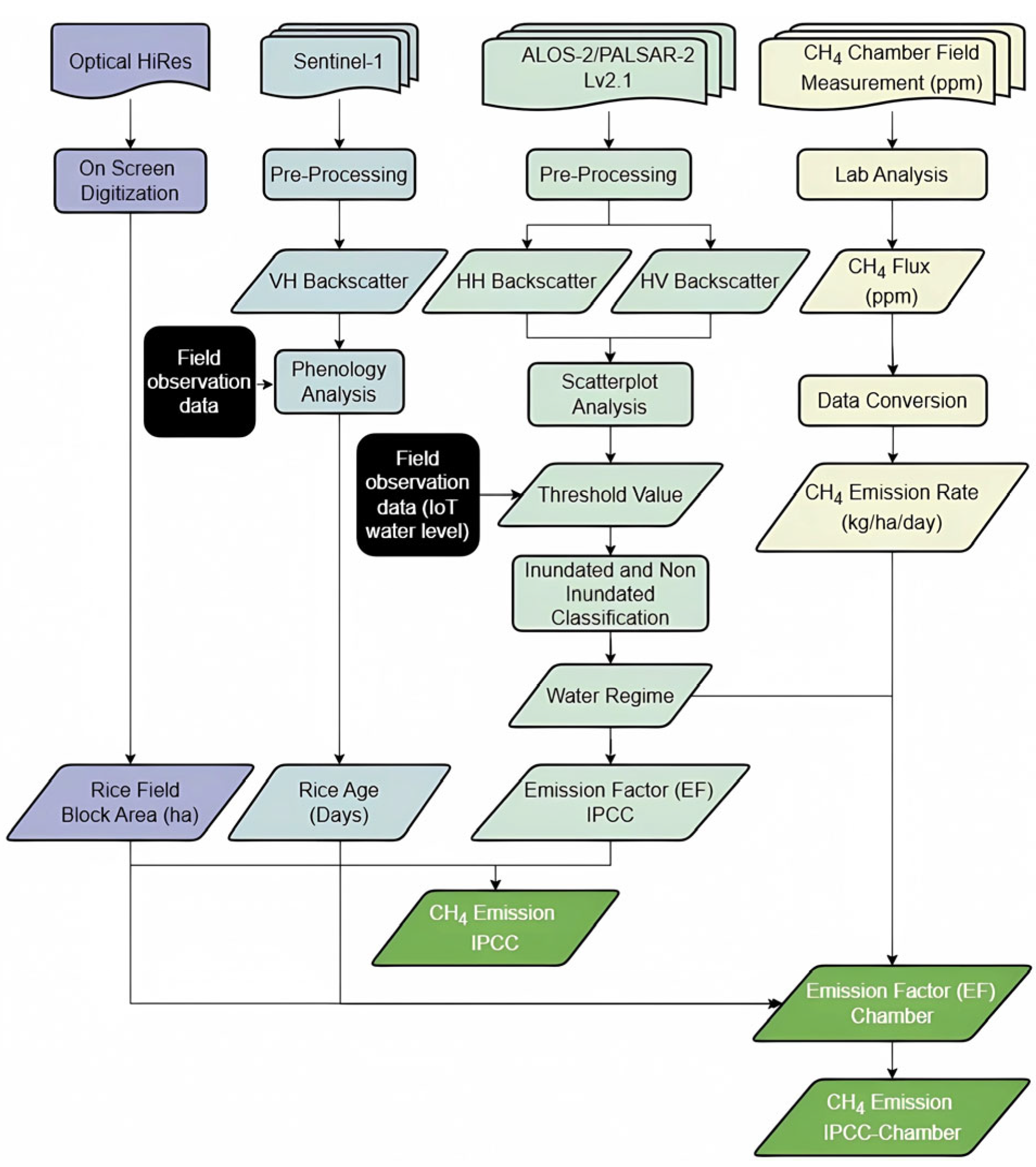
In this research, we employed the Rynan AWD Tube with a laser sensor based on Internet of Things (IoT) technology to automatically measure water levels in rice fields. The system remotely monitors water levels through a mobile app and central software management. The laser sensor operates on the light principle, with a measurement range of ±20 cm and an accuracy of ±2 cm (https://rynanagriculture.com/alternate-wetting-drying-plus (accessed on 1 February 2024)). IoT devices were installed at two AWD sites and one CF site.

2.3. Methods

2.3.1. IPCC Guidelines

This study utilized satellite remote sensing data to identify the water regime influencing emission factors, delineate rice field areas, and classify rice age for each field parcel, serving as inputs for CH₄ emission estimation. According to the IPCC 2019 guidelines, this approach falls under Tier 3 methodology, representing the highest level of detail and accuracy in emission estimation. Formula (4), used to calculate CH₄ emissions, is presented below:

CH₄ emission = Aij × Tij × EFij

(4)

where Aij is the rice cultivation area (ha), Tij is the rice age (days), and EFij is the emission factor (kg ha⁻¹ d⁻¹). CH₄ emissions from rice cultivation were expressed in the unit of kg parcel⁻¹ season⁻¹. Emission factors were then differentiated into two categories: first, the national emission factor based on Indonesian standards (

Table 1. Standard value of emission factor (EF) of methane for the world, the region of Southeast Asia, and the national scale of Indonesia.

Region	Emission Factor (EF) (kg ha−1 d−1)	Error Range (kg ha−1 d−1)	Source
World	1.19	0.80–1.76	IPCC Guidelines [2]
Southeast Asia	1.22	0.83–1.81	IPCC Guidelines [2]
Indonesia	1.61	-	Indonesian standard of CH4 emission calculation [41]

), and second, the local emission factor from field chamber-based measurement.

To calculate the national EF based on water regime differentiation, the IPCC provides scaling factors (SFw) specific to Southeast Asia and Indonesia, as summarized in

Table 2. Scaling factors for emission factor adjustments based on water regime [2].

Water Regime		Southeast Asia		Indonesia
		Scaling Factor (SFw)	Error Range	Scaling Factor (SFw)
Upland		0	-
Irrigated	Continuously flooded	1.00	0.73–1.27	1.00
	Single drainage period	0.71	0.53–0.94	0.71
	Multiple drainage periods	0.55	0.41–0.72	0.46
Rainfed and deepwater	Regular rainfed	0.54	0.39–0.74	0.49
	Drought prone	0.16	0.11–0.24	-
	Deepwater	0.06	0.03–0.12	-

. For irrigated rice fields, water regimes are classified into three categories: continuously flooded, single drainage period, and multiple drainage periods or AWD. A scaling factor of 1.0 is applied to continuously flooded conditions, while a factor of 0.55 is used for fields with multiple drainage periods. Then, it is used to calculate national CH₄ rice emissions based on the national EF and SFw (Formula (5)).

Furthermore, the calculation of the local EF is based on closed-chamber field measurement, in which CH₄ flux was differentiated into continuous flooding and alternate wetting and drying (AWD). It is referred to as SFw in the national standard for continuous flooding and multiple drainage periods, respectively. CH₄ flux is then converted into kg ha⁻¹ day⁻¹, the same unit as EF national based on IPCC guidelines. Local CH₄ rice emission is calculated based on the local EF described in Formula (6).

CH₄ rice emission national = Aij * Tij * EFnational * SFw

(5)

CH₄ rice emission local = Aij * Tij * EFlocal

(6)

where EFnational refers to EF Indonesia (Table 1), which is 1.61. SFw refers to the SF water regime in Indonesia (Table 2), which is continuous flooding and multiple drainage periods of 1.00 and 0.46, respectively. Meanwhile, the EFlocal was counted from the field measurement.

2.3.2. Rice Cultivation Mapping

High-resolution imagery from Google Earth, acquired on March 19th, 2024, was used to delineate rice cultivation areas within the study site. Natural color composite images were generated using visible bands to enhance the clarity of land cover features. A key factor in delineating rice fields is the presence of ‘pematang’ (parcel boundary), a local term for the narrow raised boundaries that separate individual fields. These features are clearly visible in high-resolution imagery and are critical for accurate parcel-level mapping, particularly in areas dominated by smallholder farms where fields are densely arranged.

2.3.3. Rice Age

Rice age in this study was estimated using VH backscatter data from Sentinel-1, with all available acquisitions from February to June 2024. VH backscatter is sensitive to rice phenological changes and was used to identify transplanting and harvesting dates. The first minimum VH backscatter value was used to determine the transplanting date, as this stage—characterized by flooded fields and young seedlings—produces a distinct low backscatter signal [42]. As the temporal VH backscatter pattern stabilized, it indicated progression toward the harvesting stage. The minimum value within this stabilized pattern was then used to identify the harvesting date [43]. After harvesting, lower backscatter values may still exist, reflecting land preparation for the next planting season. Rice age was then calculated as the interval between transplanting and harvesting dates, with an additional 20-day seedling period included. To improve accuracy, local transplanting date information provided by farmers was incorporated into the estimation process.

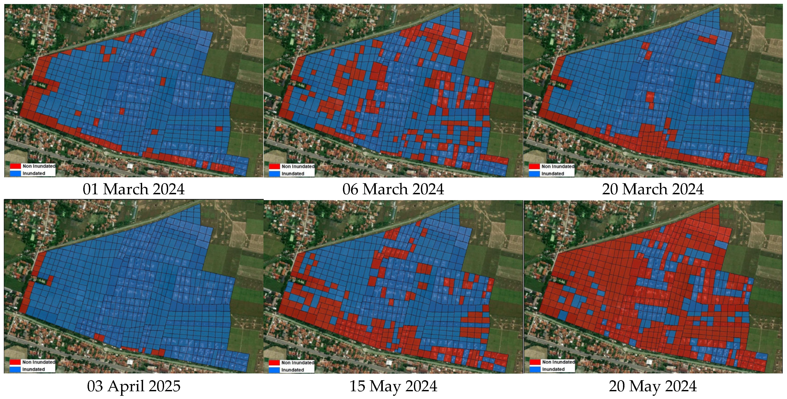
2.3.4. Identification of Inundated and Non-Inundated Areas

ALOS-2/PALSAR-2 data were used to spatially distinguish between inundated and non-inundated areas. The HH and HV backscatter data from PALSAR-2 are highly sensitive to surface water and play a key role in detecting inundation. Operating in the L-band frequency (1.2 GHz), PALSAR-2 enables deeper penetration through vegetation and soil, making it effective for identifying water bodies and flooded areas even under dense canopy cover [44]. Its dual-polarization capability (HH and HV) enhances the differentiation between surface types—such as water and land—by analyzing backscatter variations [12].

Inundated rice fields were identified using a threshold-based approach applied to HH and HV backscatter time series. Ground truth data on inundation status were collected from IoT water-level sensors installed at the experimental site. The water regime of each rice field was classified by analyzing the temporal sequence of inundated and non-inundated conditions over a single cropping season. Fields experiencing six or more inundation events were categorized as continuously flooded, while those with fewer than six events were classified as having a multiple drainage regime, consistent with the AWD practice.

2.3.5. In-Situ CH₄ Measurement Using Closed-Chamber Method

The daily CH₄ flux measurements were carried out every 2 weeks, at approximately 14, 28, 41, 56, 71, and 85 DAT, during the rice-growing seasons in two irrigation systems, AWD and CF, using a chamber equipped with a base chamber. The chamber is made of transparent plastic with a thickness of 0.8 mm and an aluminum frame (100 cm height, 50 cm width, 50 cm length) to cover four clumps of rice paddy with line spacing of 35 cm × 35 cm. The base chamber is made of aluminum (10 cm height, 50 cm width, 50 cm length), fixed at the field’s sampling point. Aluminum is commonly used for chamber materials since it is chemically unreactive with the gases being measured [45]. The size is similar to the experimental setup by [46] and [47]. Other equipment included a digital thermometer for temperature measurement, a 6-volt battery and fan to homogenize the air inside the chamber, and 10 mL vials for storing samples. In addition, walk boards were in each experimental plot to minimize the release of CH₄ gases through air bubbles (ebullition) due to pressure on the soil surface while taking samples.

GHG sampling was conducted between 06:00 to 08:00 a.m. Temperature changes in the chamber were recorded at each sampling interval: 5, 10, 15, 20, and 25 min. The headspace in the chamber was collected according to the height of the water level. Gas samples were taken in a 20 mL syringe and stored in a 10 mL vial (vacuum).

The concentration of CH₄ gas was analyzed using gas chromatography (GC) at the Agricultural Environmental Instrument Standard Testing Center of the Ministry of Agriculture in Pati, Central Java. The GC has a Flame Ionization Detector (FID) to analyze CH₄ concentration. The CH₄ fluxes and daily emissions from rice fields were calculated based on the equation adopted by [41]. Total CH₄ emissions during rice-growing seasons were calculated using the trapezoidal integration method, linear interpolation, and numerical integration between sampling times [42].

The overall data processing and analysis workflow for estimating CH₄ emissions using remote sensing data and in-situ measurements in this study is illustrated in Figure 3.

3. Results

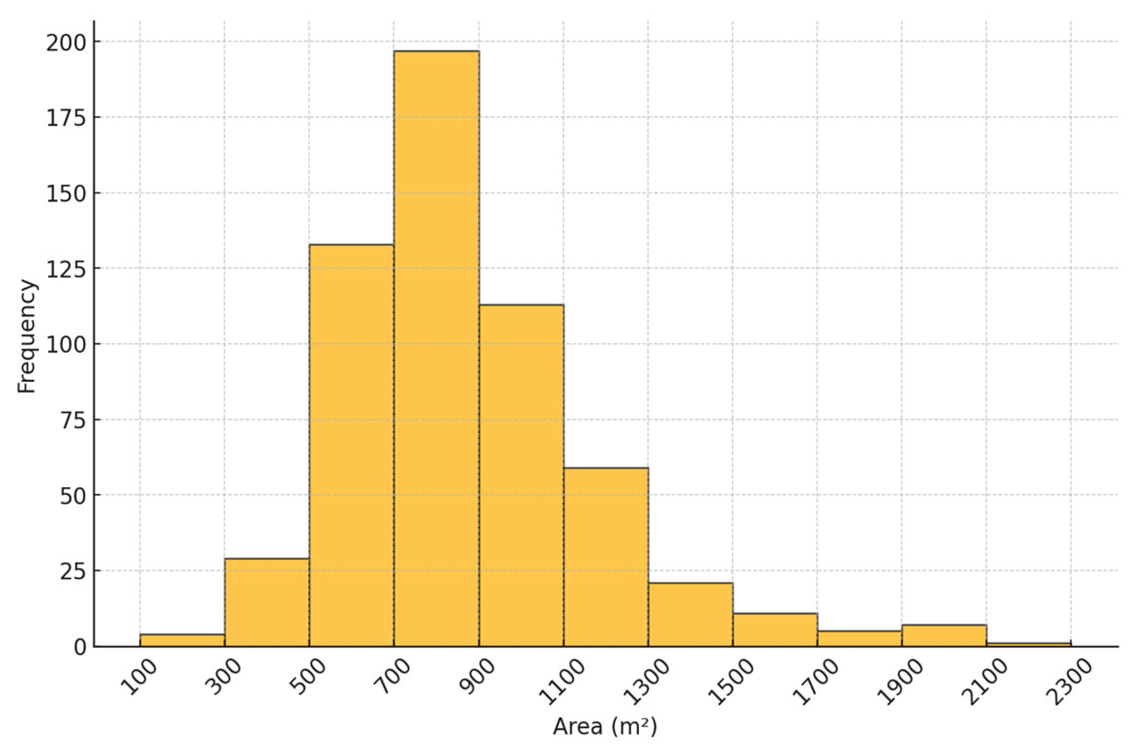
3.1. Rice Cultivation Area

A total of 580 rice field parcels (50 ha) were identified, and their areas were calculated based on high-resolution imagery. Figure 4 shows the distribution of parcel sizes in square meters. The mean field area is 871 m², and the median is 817 m², indicating a relatively symmetrical distribution. Parcel sizes range from 178 m² to 2268 m², with a standard deviation of 299 m². Most fields are clustered around the mean, with variation likely influenced by land ownership patterns and local agricultural practices. The selected AWD parcels measured 1961 m² and 2922 m², while the CF parcel measured 603 m².

3.2. Rice Age (Growing Periods)

Rice age classification was based on VH backscatter values from Sentinel-1, which are sensitive to surface water and crop structure. As shown in Figure 5a, VH backscatter values across 580 rice field parcels from February to June 2024 follow a consistent temporal pattern: low values at the beginning of the season, gradually increasing as the crop matures. Early-season backscatter values (mid-February to early March) ranged between −22 dB and −26 dB, indicating high water saturation associated with the land preparation and transplanting phase. The transplanting periods were identified by the lowest VH backscatter value, marked by the blue shading, which reflects waterlogged conditions and sparse early vegetation cover. As the rice crop developed, the VH backscatter gradually increased, reaching values between −15 dB and −18 dB, and then the pattern tended to stabilize. The harvesting periods, indicated by declining backscatter within the red shading, correspond to early to mid-June 2024 when the fields were drier and vegetation structure had peaked. These trends were consistent across all selected parcels, allowing rice age to be estimated by measuring the interval between transplanting and harvesting dates, with an additional 20-day seedling period considered in the calculation. Figure 5b–h represents field conditions from land preparation through the rice crop growth stages, including the transplanting, vegetative, and generative stages, respectively.

Figure 6 shows the spatial distribution of transplanting dates and rice age across the study area, derived from multitemporal Sentinel-1 VH backscatter data. The maps show a temporal variation in paddy field preparation and planting activities. The earliest transplanting was recorded on 1 February 2024, while the latest transplanting occurred around 26 March 2024. The transplanting phases continue from 1, 10, 22, and 26 February 2024, primarily in the central and northeastern sections. In contrast, the latest transplanting dates—6, 17, 20, and 26 March 2024—were more concentrated along the field edges and scattered patches, indicating variability in planting schedules across the study area.

The total growing periods of rice in the study area vary across different field parcels, ranging from 101 to 125 days from seedling to harvest or the equivalent of 81 to 105 DAT. The rice seedlings were nurtured in nurseries for 20 days before being transplanted into the field. The spatial distribution of rice age shows significant variation, with shorter growth periods (101–104 days) primarily observed in the northeastern and southeastern sections, while longer growth periods (116–125 days) are more concentrated in the central and western regions.

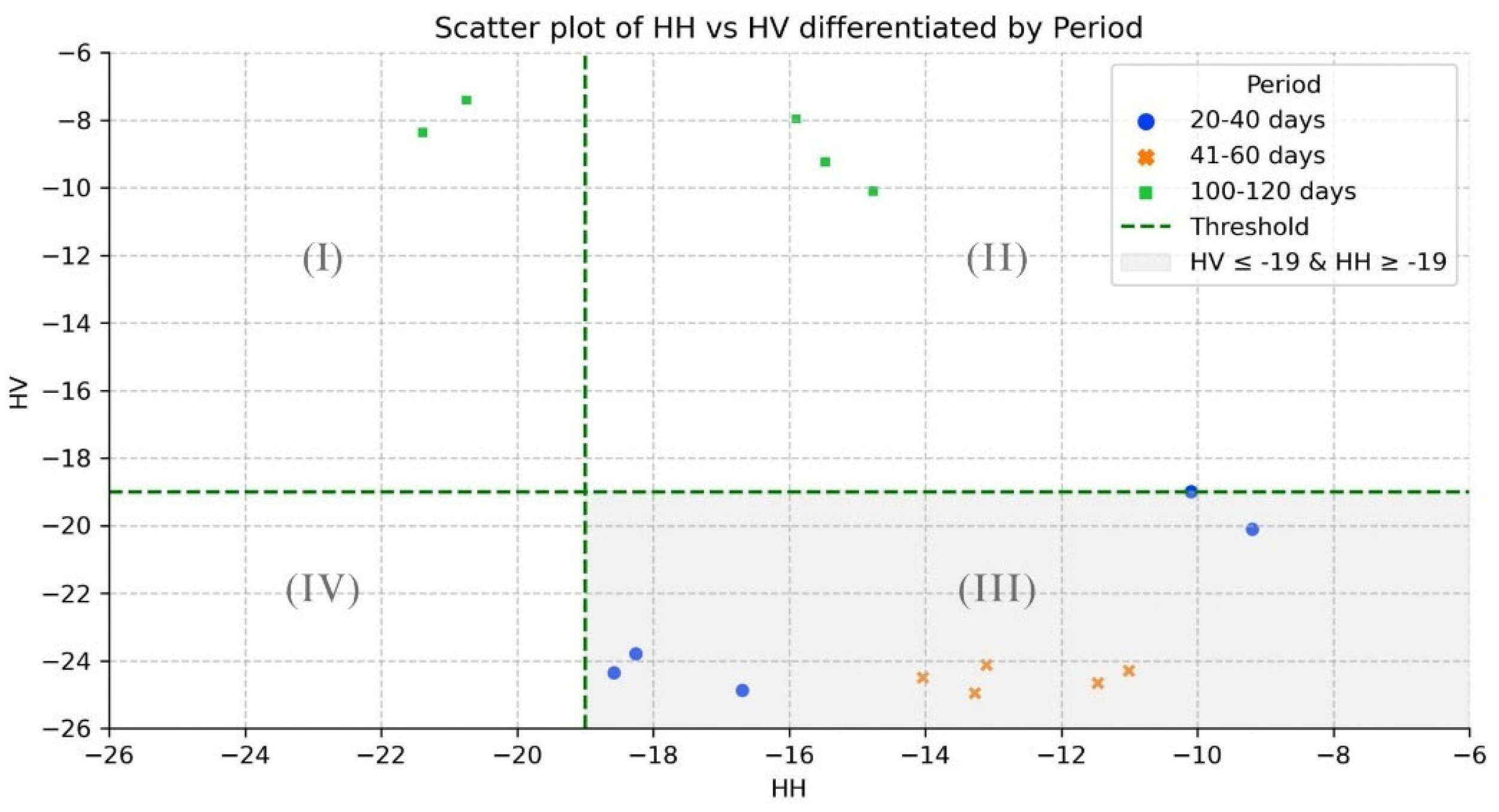
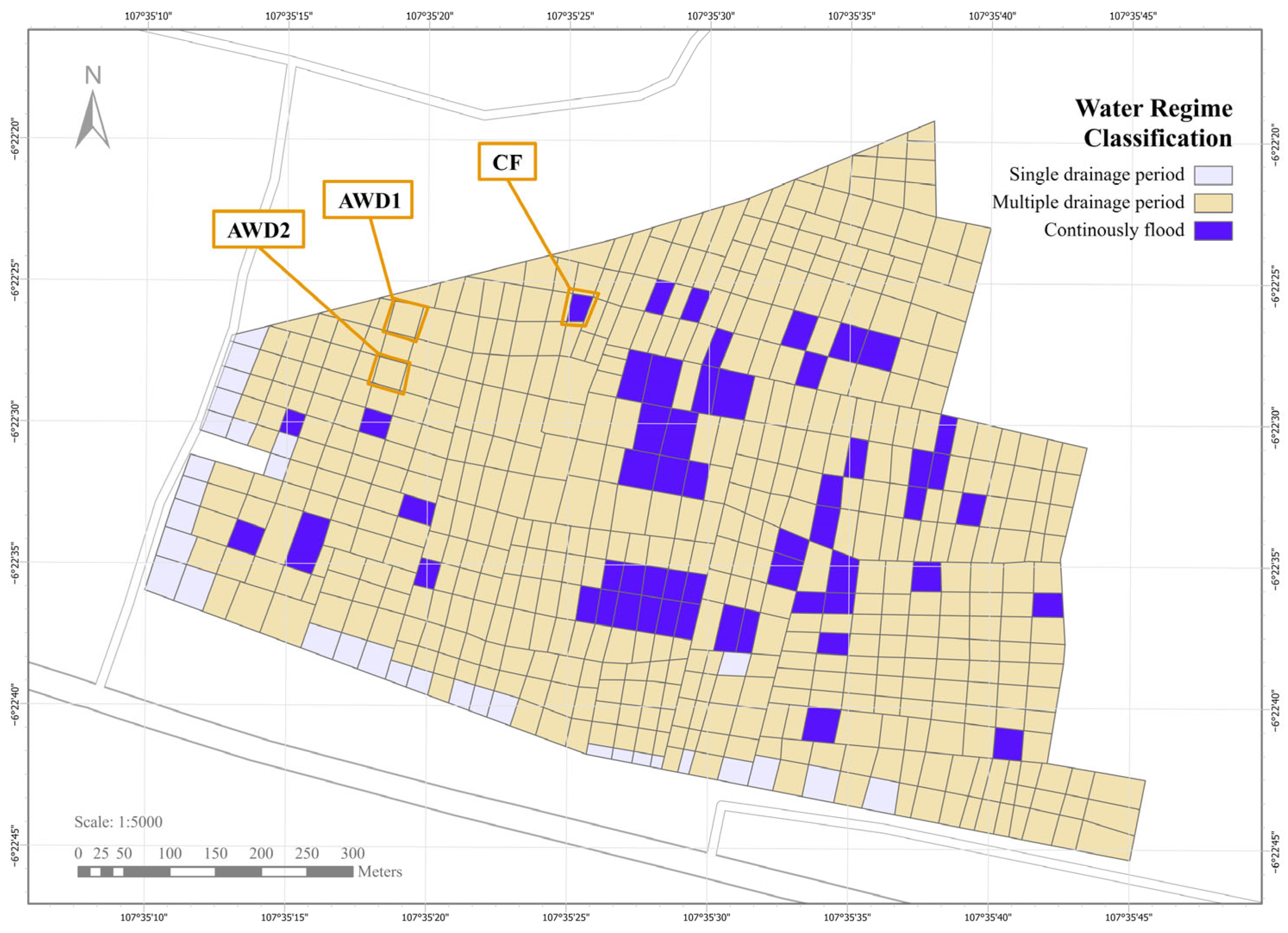
3.3. Water Regime Characterization Using ALOS-2/PALSAR-2 Backscatter and IoT Water Level Observations

The inundation dynamics of rice fields within the study area were analyzed using dual-polarization HH and HV backscatter data obtained from ALOS-2/PALSAR-2. Figure 7 presents a scatter plot of HH versus HV backscatter values, with data points color-coded according to rice growth stages: 20–40, 41–60, and 100–120 DAT. Each data point represents the mean HH and HV values calculated from three monitored parcels, with six samples collected per growth stage, based on SAR images acquired between February and May 2024.

Water level measurements obtained from IoT sensors installed across the parcels were utilized to validate and support the interpretation of inundation conditions. The statistical summary of water levels for each growth stage is provided in

Table 3. Water level statistics based on IoT measurements during rice growth stages.

Period (Days)	Mean Water Level (mm)	Minimum (mm)	Maximum (mm)	Number of Samples
20–40	49	10	87	6
41–60	35	−2	80	6
100–120	−49	−180	16	6

. During the early growth stages (20–40 and 41–60 DAT), IoT measurements indicated mean water levels of approximately 49 mm and 35 mm, respectively, with maximum recorded depths reaching up to 87 mm. In contrast, during the later growth stage (100–120 DAT), the mean water level decreased to –49 mm, suggesting dry conditions or water recession below the surface.

Figure 7 aids in identifying a robust threshold for distinguishing inundated and non-inundated fields: inundated rice fields consistently exhibited HV backscatter values of ≤−19 dB combined with HH backscatter values of ≥−19 dB. Data points representing these conditions clustered within Quadrant III, corresponding to periods of confirmed surface inundation based on IoT water level measurements. Quadrants I and II predominantly contained data points corresponding to 100–120 DAT, aligning with non-inundated field conditions. No observations were recorded in Quadrant IV, further reinforcing the clear separation between inundated and non-inundated states.

The inundation status of experimental rice fields during the wet season was analyzed over six ALOS-2/PALSAR-2 observation periods (Figure 8). At the early stage of the crop season (1 March 2024), most fields were identified as inundated (blue color), whereas fields near settlements were classified as non-inundated (red color). Some areas began to dry in the next 5 days, particularly in the center and north of the study site. This change is attributed to the implementation of AWD practice, which regulates water levels and reduces continuous flooding in the field.

Based on the water regime classification that resulted in Figure 8, we produced Figure 9, which illustrates the spatial classification of water regimes in a rice field over one cropping season. The water regime was categorized into single drainage periods (gray), multiple drainage periods (orange), and continuously flooded conditions (blue). This research only considers the multiple drainage periods and continuous flooding, which were validated using IoT water level devices. Two locations of IoT devices were located in AWD irrigation practices (AWD1 and AWD2), and the IoT device in another location represented the CF practice. Each location was observed six times, matched with the ALOS-2/PALSAR-2 acquisition date, during one cropping season. The distribution of water regimes indicates variability in irrigation management, with continuously flooded areas predominantly concentrated in specific sections, while multiple drainage period areas are more widely dispersed. Continuously flooded areas are primarily concentrated in the central part of the study area, whereas multiple drainage periods are more common in the outer regions. The area’s topography influences this distribution, as the central region is at a lower elevation than its surroundings, allowing water to accumulate and remain flooded for longer durations.

3.4. Emission Factor Local (EFlocal) Using Closed-Chamber Method

Table 4. Daily fluxes and total CH₄ emissions from closed-chamber.

Treatments		Daily Fluxes of CH4 mg CH4 m−2 Days−1						Total	Average
		14 DAT	28 DAT	41 DAT	56 DAT	71 DAT	85 DAT	(kg ha−1 Season−1)
AWD1	I	42.10	133.03	7.40	0.19	15.02	0.00	27.10	27.97
	II	15.98	12.75	157.43	2.71	2.66	16.38	28.84
AWD2	I	95.67	215.23	50.50	3.43	0.00	5.69	50.74	41.21
	II	18.34	103.02	84.77	5.18	9.29	9.70	31.68
CF	I	243.35	1227.33	914.10	0.00	336.30	27.50	379.93	292.74
	II	343.61	247.95	348.11	133.79	353.69	31.04	205.55

presents the daily fluxes of CH₄ emissions during the rice-growing season in February–May 2024 with the glutinous rice varieties using the closed-chamber method. The result shows different flux dynamics for AWD and CF irrigation systems. The pattern of daily CH₄ fluxes in the season increased CH₄ emissions at 14, 28, and 41 DAT. On the other hand, at 56 DAT, there was a dramatic decrease in the fluxes, even though the rice growth phase was early in the generative phase with the maximum number of tillers. Daily fluxes decreased at 71 and 85 DAT due to the plant’s growth into filling and ripening seeds before harvest, where photosynthesis results were more translocated to rice seeds. At 14, 28, and 41 DAT, the AWD1 and AWD2 treatments have a range of daily fluxes of CH₄ that are lower than the CF.

Regarding the daily flux of CH₄ at 56, 71, and 85 DAT, there were problems during sample measurement, such as the difficulty of covering four clumps in a chamber. The increasing height, the number of tillers, and the addition of the root volume of rice caused leakage during gas sampling. The calculation of total CH₄ emissions of AWD treatments showed average total emissions of 27.97 and 41.21 kg ha⁻¹ season⁻¹, while in the CF treatment, it was 292.74 kg ha⁻¹ season⁻¹. Applying an AWD water management system with glutinous rice varieties in the season reduced CH₄ emissions by 85.92–90.44%.

Table 5. Comparison of CH₄ emission factors from Indonesia’s national standard and local closed-chamber measurements under different water regimes.

Water Regime	Emission Factor (kg ha−1 Day−1)
	Indonesia (EFnational × SFw National)	Chamber (EFlocal)
Continuous Flooding	1.61 × 1.00 = 1.61	2.97
Multiple drainages or AWD	1.61 × 0.46 = 0.74	0.78

presents CH₄ emission factors for different water regimes, comparing values from Indonesia’s national standard with locally measured data using the closed-chamber method. Under CF, local measurements indicate a significantly higher emission factor (2.97 kg ha⁻¹ day⁻¹) than the national standard (1.61 kg ha⁻¹ day⁻¹). Meanwhile, the local measurement (0.78 kg ha⁻¹ day⁻¹) under multiple drainage conditions or AWD is slightly lower than the national standard value (0.88 kg ha⁻¹ day⁻¹).

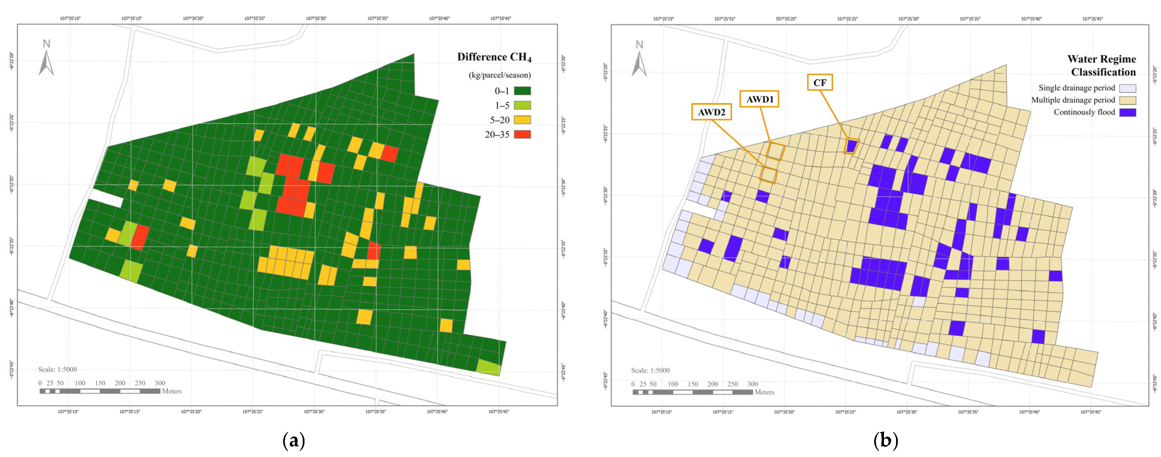
3.5. Spatial Distributions of CH₄ Emission

Figure 10 presents CH₄ emissions estimated using two different EFs: (a) EFnational and (b) Eflocal, which could be called CH₄ national and CH₄ local, respectively. The CH₄ national approach shows that most rice fields emit methane within the 1–10 kg range, with a few plots exhibiting higher emissions between 15 and 50 kg. The highest concentrations are observed in specific areas, particularly in the central and southwestern sections, indicated by orange and red color shades. Overall, the spatial distribution of CH₄ emissions using the EFnational factor appears relatively uniform, with only a few localized areas showing elevated emissions.

Meanwhile, the CH₄ local approach shows a broader emission range from 1–75 kg. The EFlocal approach spatial distribution displays are quite similar to the EFnational; only a few locations have higher emissions. Higher emissions are located in the central and southwestern parts, which are shaded in blue. Also, the southern part has higher emissions, as shown in the orange and color shades. The site with higher emissions is at a lower elevation, resulting in persistent water coverage or increased water accumulation. It is a CF site. The differences between the two emission factors suggest that the EFlocal method tends to produce higher than the EFnational, likely capturing finer-scale variations in field conditions, especially for CF fields.

Figure 11 presents the spatial distribution of CH₄ emission differences between national and local emission factors (Figure 11a) to the water regime classification of the study area (Figure 11b). The emission differences vary across the field, with higher emission (20–35 kg CH₄/parcel/season) observed predominantly in areas under CF, as indicated by the red zones in Figure 11a. In contrast, fields managed under AWD regimes, particularly AWD1 and AWD2, exhibit lower CH₄ emission differences, primarily within the 0–5 kg CH₄/parcel/season range (dark green and light green zones).

4. Discussion

This study investigated the potential of using satellite data to provide the spatial distribution of CH₄ emissions from rice paddy cultivation in Subang, West Java. Multisensor satellite data were used to determine key parameters, including rice cultivation areas, rice age, and water regime, which are essential for estimating the spatial variation of CH₄ emissions under different water management practices such as AWD and CF. Integrating Sentinel-1 SAR for rice phenology and ALOS-2/PALSAR-2 for water regime classification allowed for a detailed spatial representation of the EF. Additionally, in-situ CH₄ flux measurements using the closed-chamber method were used for pattern validation, though not for direct quantity comparison. Below is a detailed discussion of the study’s findings, limitations, and future research direction

4.1. Rice Age Estimation Using Sentinel-1 SAR

Sentinel-1 SAR data provided reliable rice age estimation due to its high temporal resolution (12 days), which is crucial for capturing phenological changes such as transplanting and harvesting. In this research study, the area located in two scenes of Sentinel-1 makes the period difference less than 12 days (9 and 3 days). The identification of transplanting dates based on the lowest VH backscatter values aligns with previous studies [43,48,49], that demonstrate the effectiveness of SAR backscatter in tracking rice growth stages, especially VH backscatter, in identifying rice growth stages [48]. This method aligns with the approach used in this study, especially for transplanting and harvesting dates, as well as field data from farmer interviews. The backscatter variation of VH during transplanting was observed as the lowest, reflecting the inundated condition of rice fields. However, this method has limitations in accuracy due to the 12-day revisit cycle of Sentinel-1, which may introduce uncertainties when distinguishing closely spaced planting events in one scene Sentinel-1 study location.

4.2. Water Regime Classification Using ALOS-2/PALSAR-2

ALOS-2/PALSAR-2 imageries were utilized to classify water regimes by analyzing HH and HV backscatter, allowing the differentiation between CF and AWD irrigation practices. The L-band radar data demonstrated stable sensitivity to inundation conditions, consistent with previous studies using polarimetric SAR to detect waterlogged agricultural fields. The L-band backscattering coefficient remains persistently sensitive in detecting inundated rice paddies following irrigation events, regardless of vegetation growth or characteristics [33]. Tamkuan and Nagai, 2021 [50] studied the use of ALOS-2/PALSAR-2 images for flood detection. HH and HV polarization in the L-band performs better in paddy field water identification than in the C-band. Similarly, the combination of L-band HH and HV can assess waterlogging conditions, as their variations correspond to changes in local elevation [32]. The spatial variability of water regimes significantly influenced CH₄ emissions, with CF areas exhibiting consistently higher emission levels due to prolonged anaerobic conditions favoring methanogenesis. Time-series data of inundated and non-inundated fields in the crop season period has been used to differentiate AWD and CF fields.

4.3. Comparison of Local Emission Factor (EFlocal) and National Standard (EFnational)

One of the key contributions of this study is the estimation of a locally specific emission factor (EFlocal), which was found to be higher than the national standardized EF (EFnational). The national EF, derived from broader regional averages, does not account for micro-scale variations in soil pH, soil organic carbon (SOC) content, pre-season water management, water regime, organic amendment application, climate, and varieties [8,51]. In contrast, the closed-chamber method provided precise, field-specific CH₄ flux measurements, demonstrating that CF plots emitted significantly higher CH₄ compared to AWD plots. The higher EFlocal values can be attributed to specific local factors such as land conditions, rice variety, agricultural practices, and irrigation methods, which are not captured in national-scale estimates. These findings suggest that adopting locally refined EFs could enhance the accuracy of CH₄ inventories and support more effective mitigation policies.

The integration of high-resolution imagery and chamber-based flux measurements enables precise, spatially explicit estimation of CH₄ emissions at the parcel level. Using 30 cm resolution Google Earth imagery, we accurately delineated individual rice fields, including the narrow “pematang” boundaries characteristic of smallholder landscapes. This detailed mapping ensures that the area variable in the emission equations reflects the actual size of each parcel. Meanwhile, chamber measurements were conducted within these same delineated parcels, allowing the local emission factor to represent field-specific conditions. Because both area and emission factor data are derived at the same spatial resolution, they can be directly integrated in Equations (4) and (6) to estimate methane emissions for each parcel. This spatial alignment preserves local variability in field boundaries and emission rates, which is essential for accurately identifying emission hotspots and understanding the effects of different management practices. By combining high-resolution parcel mapping with localized emission factors, our approach effectively captures the spatial heterogeneity of CH₄ emissions across the study area.

4.4. Spatial Distribution of CH₄ Emissions

The spatial distribution of CH₄ emissions varied significantly between CH₄ national and CH₄ local, which was estimated using the EFnational and EFlocal, respectively. The CH₄ national approach produced relatively uniform CH₄ emission estimates, whereas the EFlocal demonstrated greater spatial variability, reflecting the influence of local field conditions. The highest CH₄ emissions were concentrated in topographically low-lying areas where the CF practice was implemented, as indicated by the DEMNAS imagery of the study area. This highlights the importance of spatially explicit emission modeling. AWD irrigation resulted in lower emissions and less difference between national and local approaches. Meanwhile, CF areas showed significantly higher CH₄ emissions than AWD, and CF has higher differences between national and local approaches. Comparisons with previous remote sensing–based CH₄ studies suggest that integrating local measurements into satellite-based models significantly improves accuracy [52], making this approach highly applicable for national and regional emission assessments.

The increasing CH₄ emissions in paddy fields are influenced by various factors, such as water regime, organic matter addition, soil temperature, soil moisture, fertilizer use, and rice variety [53,54]. Water management is the dominant factor in the release of CH₄ emissions in paddy fields. CF practice creates water-saturated, reductive, and anoxic soil conditions. This condition increases the formation of CH₄ by Archaea methanogens that utilize carbon sources in the soil [55]. These CH₄ emissions are translocated through the aerenchyma tissues of rice to the atmosphere [56]. The way to reduce GHG emissions in paddy fields is through water management with AWD. It reduced CH₄ emissions by between 29% and 70% [53,57]. The amount of CH₄ emissions is influenced by the height of the water level and the long time paddy fields are flooded, which increases the concentration of CH₄ released. The wet and dry cycle also affects water retention and root uptake, increasing nutrient availability and supporting plant growth [58]. AWD conditions enhance plant adaptation to develop root growth, affect gene expression related to root morphology and physiology, and facilitate deeper root systems [59]. In addition, the use of rice varieties is also a factor affecting CH₄ emissions. Rice varieties have larger medullary cavities in rice roots that can enhance gas transport in larger leaf areas, contributing to higher transpiration rates, stomatal conductance, and the frequency of stomatal opening and closing in regulating CH₄ release from the plant to the atmosphere [60]. Root characteristics, including root volume and oxidation activity, are inversely correlated with CH₄ emissions, suggesting that a robust root system can mitigate emissions [61].

4.5. Study Limitations and Future Research

Several limitations were identified in the remote sensing analysis of rice phenology and water regime, which may contribute to uncertainty in the spatial distribution of CH₄ emission estimation in the study area. In the phenological analysis based on Sentinel-1 imagery, only VH polarization was utilized; incorporating VV polarization or applying VH/VV ratio analysis could potentially enhance sensitivity to different rice growth stages. Future studies should explore multi-polarization approaches to improve phenological stage classification accuracy, which would, in turn, refine the temporal scaling of emission estimates.

For water regime mapping using ALOS-2/PALSAR-2 data, the current study was limited to dual-polarization (HH and HV) acquisitions and employed a simple threshold-based classification method. Future research could leverage full-polarization (quad-pol) ALOS-2 data to capture more detailed scattering mechanisms associated with inundation conditions. Additionally, integrating a greater number of IoT-based water level sensors across a broader spatial distribution would strengthen ground validation efforts. Implementing advanced classification techniques, such as machine learning-based or automated thresholding algorithms, could further enhance the accuracy of inundation detection. Improvements in water regime mapping are essential to better quantify emission factors linked to field flooding conditions.

Regarding CH₄ emission factor (EF) estimation, the current study requires additional sampling across different planting seasons to improve robustness. The EF and scaling factor estimations are currently based on Tier 2 IPCC guidelines, which primarily account for water regime variations but do not incorporate other influential factors such as soil type, fertilizer application, and rice variety. Transitioning toward a Tier 3 methodology by integrating more extensive spatial and agronomic data will enhance the accuracy and representativeness of CH₄ emission estimates.

The seasonal nature of the current data collection also means that interannual variability in climate and agricultural practices was not fully captured. While water management was considered, other variables influencing CH₄ emissions, such as soil characteristics, organic amendments, and fertilizer types, were not explicitly modeled. Future research should expand sampling across multiple cropping seasons and integrate additional agronomic factors to develop a more comprehensive Tier 3 IPCC-compliant emission model. Furthermore, applying machine learning techniques to classify remote sensing data could improve the precision of both surface water detection and emission modeling.

5. Conclusions

This study assessed the potential of applying multisensor satellite data—namely Sentinel-1, ALOS-2/PALSAR-2, and high-resolution optical imagery—for developing a spatial model of CH₄ emission estimation in rice paddy fields, following IPCC guidelines. The 6-day VH polarization time series from the Sentinel-1 constellation provided useful information for identifying key rice phenological stages. The L-band data from ALOS-2/PALSAR-2 demonstrated sensitivity to surface inundation, supporting the classification of water regimes into AWD and CF practice, which are critical inputs for determining emission factors for CH₄ emission estimation. These satellite-derived variables were combined with national (EFnational) and locally measured (EFlocal) emission factors—obtained through the closed-chamber method—to represent site-specific emission characteristics in Subang, West Java. Overall, the study highlights the potential of remote sensing approaches as a complementary tool for spatial CH₄ emission modeling under varying water management practices.

The comparison between national and local CH₄ emission estimates underscores the importance of using spatially detailed emission factors, especially in rice cultivation systems. While both approaches yielded similar emission levels in AWD-dominated areas, notable differences were observed in CF fields due to variations in emission factor values. Local EF-based estimates captured a broader emission range—reaching up to 70 kg per parcel per season—compared to the more moderate levels derived from the national EF. In AWD fields, emissions remained consistently low (0–5 kg) across both approaches, whereas CF fields exhibited higher variability and greater differences. These findings suggest that incorporating locally measured emission factors and field-level water management data can enhance the accuracy of CH₄ emission assessments in agricultural landscapes. Further work exploring the impact of different soil types and rice varieties on emissions is recommended for advancing studies on remote sensing–based CH₄ emission estimation using IPCC data for further advanced SFw variables. Process automation would also be valuable for tracking variations in emissions over time.

References

1. Conrad, R. The Global Methane Cycle: Recent Advances in Understanding the Microbial Processes Involved. Environ. Microbiol. Rep. 2009, 1, 285–292. [Google Scholar] [CrossRef] [PubMed]
2. IPCC. 2019 Refinement to the 2006 IPCC Guidelines for National Greenhouse Gas Inventories Volume 4 Agriculture, Forestry and Other Land Use Chapter 5 Cropland; IPCC: Hayama, Japan, 2019. [Google Scholar]
3. Wang, Y.; Tao, F.; Chen, Y.; Yin, L. Mapping Irrigation Regimes in Chinese Paddy Lands through Multi-Source Data Assimilation. Agric. Water Manag. 2024, 304, 109083. [Google Scholar] [CrossRef]
4. FAO. World Food and Agriculture—Statistical Yearbook 2020; FAO: Rome, Italy, 2020; ISBN 978-92-5-133394-5. [Google Scholar]
5. Velthof, G.L.; van Bruggen, C.; Groenestein, C.M.; de Haan, B.J.; Hoogeveen, M.W.; Huijsmans, J.F.M. A Model for Inventory of Ammonia Emissions from Agriculture in the Netherlands. Atmos. Environ. 2012, 46, 248–255. [Google Scholar] [CrossRef]
6. Alhashim, R.; Deepa, R.; Anandhi, A. Environmental Impact Assessment of Agricultural Production Using LCA: A Review. Climate 2021, 9, 164. [Google Scholar] [CrossRef]
7. Yan, X.; Akiyama, H.; Yagi, K.; Akimoto, H. Global Estimations of the Inventory and Mitigation Potential of Methane Emissions from Rice Cultivation Conducted Using the 2006 Intergovernmental Panel on Climate Change Guidelines. Glob. Biogeochem. Cycles 2009, 23, GB2002. [Google Scholar] [CrossRef]
8. Rashid, M.A.; Bastami, M.S.; Bakar, N.A.A.; Jumat, F.; Suptian, M.F.M.; Rahman, M.H.A.; Azmin, A.A.; Talib, S.A.A. Development of National Emission Factor for Rice Production System in Malaysia: A Step Toward Achieving Sustainable Development Goals. J. Lifestyle SDG’S Rev. 2024, 5, e02774. [Google Scholar] [CrossRef]
9. Asch, F.; Johnson, K.; Vo, T.B.T.; Sander, B.O.; Duong, V.N.; Wassmann, R. Varietal Effects on Methane Intensity of Paddy Fields under Different Irrigation Management. J. Agron. Crop. Sci. 2023, 209, 876–886. [Google Scholar] [CrossRef]
10. Chidthaisong, A.; Cha-un, N.; Rossopa, B.; Buddaboon, C.; Kunuthai, C.; Sriphirom, P.; Towprayoon, S.; Tokida, T.; Padre, A.T.; Minamikawa, K. Evaluating the Effects of Alternate Wetting and Drying (AWD) on Methane and Nitrous Oxide Emissions from a Paddy Field in Thailand. Soil Sci. Plant Nutr. 2018, 64, 31–38. [Google Scholar] [CrossRef]
11. Li, L.; Li, F.; Dong, Y. Greenhouse Gas Emissions and Global Warming Potential in Double-Cropping Rice Fields as Influenced by Two Water-Saving Irrigation Modes in South China. J. Soil Sci. Plant Nutr. 2020, 20, 2617–2630. [Google Scholar] [CrossRef]
12. Arai, H.; Takeuchi, W.; Oyoshi, K.; Nguyen, L.D.; Inubushi, K. Estimation of Methane Emissions from Rice Paddies in the Mekong Delta Based on Land Surface Dynamics Characterization with Remote Sensing. Remote Sens. 2018, 10, 1438. [Google Scholar] [CrossRef]
13. Jang, S.; Park, J.; Lee, H.; Gou, J.; Song, I. Assessing Paddy Methane Emissions through the Identification of Rice and Winter Crop Areas Using Sentinel-2 Imagery in Korea. Paddy Water Environ. 2024, 22, 401–414. [Google Scholar] [CrossRef]
14. Liang, R.; Zhang, Y.; Hu, Q.; Li, T.; Li, S.; Yuan, W.; Xu, J.; Zhao, Y.; Zhang, P.; Chen, W.; et al. Satellite-Based Monitoring of Methane Emissions from China’s Rice Hub. Environ. Sci. Technol. 2024, 58, 23127–23137. [Google Scholar] [CrossRef] [PubMed]
15. Sawettachat, S.; Routray, J.K.; Preeda, P.; Tripathi, N.K. Remote Sensing Modeling for Estimating Methane Gas Emission from Irrigated Paddy Fields in Thailand. Int. J. Appl. Environ. Sci. 2010, 5, 813–831. [Google Scholar]
16. Tang, F.H.M.; Nguyen, T.H.; Conchedda, G.; Casse, L.; Tubiello, F.N.; Maggi, F. CROPGRIDS: A Global Geo-Referenced Dataset of 173 Crops. Sci. Data 2024, 11, 413. [Google Scholar] [CrossRef]
17. Zhao, Z.; Dong, J.; Zhang, G.; Yang, J.; Liu, R.; Wu, B.; Xiao, X. Improved Phenology-Based Rice Mapping Algorithm by Integrating Optical and Radar Data. Remote Sens. Environ. 2024, 315, 114460. [Google Scholar] [CrossRef]
18. Chen, N.; Yu, L.; Zhang, X.; Shen, Y.; Zeng, L.; Hu, Q.; Niyogi, D. Mapping Paddy Rice Fields by Combining Multi-Temporal Vegetation Index and Synthetic Aperture Radar Remote Sensing Data Using Google Earth Engine Machine Learning Platform. Remote Sens. 2020, 12, 2992. [Google Scholar] [CrossRef]
19. Zhao, R.; Li, Y.; Ma, M. Mapping Paddy Rice with Satellite Remote Sensing: A Review. Sustainability 2021, 13, 503. [Google Scholar] [CrossRef]
20. Kustiyo; Rochmatuloh; Saputro, A.H.; Kushardono, D. Developing the Temporal Composite of Sentinel-1 SAR Data to Identify Paddy Field Area in Subang, West Java. In Proceedings of the Sixth International Symposium on LAPAN-IPB Satellite, Bogor, Indonesia, 17–18 September 2019; Volume 11372, p. 113720H. [Google Scholar]
21. Fatchurrachman; Rudiyanto; Soh, N.C.; Shah, R.M.; Giap, S.G.; Setiawan, B.I.; Minasny, B. High-Resolution Mapping of Paddy Rice Extent and Growth Stages across Peninsular Malaysia Using a Fusion of Sentinel-1 and 2 Time Series Data in Google Earth Engine. Remote Sens. 2022, 14, 1875. [Google Scholar] [CrossRef]
22. Gao, Y.; Pan, Y.; Zhu, X.; Li, L.; Ren, S.; Zhao, C.; Zheng, X. FARM: A Fully Automated Rice Mapping Framework Combining Sentinel-1 SAR and Sentinel-2 Multi-Temporal Imagery. Comput. Electron. Agric. 2023, 213, 108262. [Google Scholar] [CrossRef]
23. Muradi, H.; Domiri, D.D.; Parsa, I.M.; Yoga, I.K.; Bustamam, A.; Rarasati, A.; Harini, S.; Manalu, R.J.; Subehi, M. Rice Phenology Classification Model Based on Sentinel-1 Using Machine Learning Method on Google Earth Engine. Can. J. Remote Sens. 2024, 50, 2368036. [Google Scholar] [CrossRef]
24. Du, M.; Huang, J.; Wei, P.; Yang, L.; Chai, D.; Peng, D.; Sha, J.; Sun, W.; Huang, R. Dynamic Mapping of Paddy Rice Using Multi-Temporal Landsat Data Based on a Deep Semantic Segmentation Model. Agronomy 2022, 12, 1583. [Google Scholar] [CrossRef]
25. Thorp, K.R.; Drajat, D. Deep Machine Learning with Sentinel Satellite Data to Map Paddy Rice Production Stages across West Java, Indonesia. Remote Sens. Environ. 2021, 265, 112679. [Google Scholar] [CrossRef]
26. Tamilmounika, R.; Muthumanickam, D.; Pazhanivelan, S.; Ragunath, K.P.; Kumaraperumal, R.; Sivamurugan, A.P.; Satheesh, S.; Sudarmanian, N.S. Quantifying Methane Emissions in Major Rice Growing Areas of Tamil Nadu Using Remote Sensing and Land Surface Temperature Model. Plant Sci. Today 2024, 11, 5604. [Google Scholar] [CrossRef]
27. Shi, Y.; Lou, Y.; Zhang, Z.; Ma, L.; Ojara, M.A. Estimation of Methane Emissions Based on Crop Yield and Remote Sensing Data in a Paddy Field. Greenh. Gases Sci. Technol. 2020, 10, 196–207. [Google Scholar] [CrossRef]
28. Sasai, T.; Nakai, S.; Ono, K.; Mano, M.; Miyata, A. Estimation of Methane Emission from Rice Paddy Soils in Japan Using the Diagnostic Ecosystem Model. J. Agric. Meteorol. 2017, 73, 133–139. [Google Scholar] [CrossRef]
29. Torbick, N.; Salas, W.; Chowdhury, D.; Ingraham, P.; Trinh, M. Mapping Rice Greenhouse Gas Emissions in the Red River Delta, Vietnam. Carbon Manag. 2017, 8, 99–108. [Google Scholar] [CrossRef]
30. Ouyang, Z.; Jackson, R.B.; McNicol, G.; Fluet-Chouinard, E.; Runkle, B.R.K.; Papale, D.; Knox, S.H.; Cooley, S.; Delwiche, K.B.; Feron, S.; et al. Paddy Rice Methane Emissions across Monsoon Asia. Remote Sens. Environ. 2023, 284, 113335. [Google Scholar] [CrossRef]
31. Phan, H.; Toan, T.L.; Bouvet, A. Understanding Dense Time Series of Sentinel-1 Backscatter from Rice Fields: Case Study in a Province of the Mekong Delta, Vietnam. Remote Sens. 2021, 13, 921. [Google Scholar] [CrossRef]
32. Hoshikawa, K.; Phontusang, P.; Katawatin, R. Synthetic Aperture Radar Polarised Backscattering Behaviour in Partially Inundated Agricultural Fields. Eur. J. Remote Sens. 2023, 56, 2269305. [Google Scholar] [CrossRef]
33. Bazzi, H.; Baghdadi, N.; Charron, F.; Zribi, M. Comparative Analysis of the Sensitivity of SAR Data in C and L Bands for the Detection of Irrigation Events. Remote Sens. 2022, 14, 2312. [Google Scholar] [CrossRef]
34. BPS. Provinsi Jawa Barat Dalam Angka 2024; The Central Bureau of Statistics: Bandung, Indonesia, 2024. [Google Scholar]
35. Leopold, L.B.; Wolman, M.G.; Miller, J.P.; Wohl, E.E. Fluvial Processes in Geomorphology; Dover Publications: Garden City, NY, USA, 2020; ISBN 0-486-84552-4. [Google Scholar]
36. Indonesian Ministry of Energy and Mineral Resources. Geological Map of Remote Sensing Image Interpretation Pamanukan Sheet, West Java. Available online: https://geologi.esdm.go.id/geomap/pages/preview/peta-geologi-interpretasi-citra-inderaan-jauh-lembar-pamanukan-jawa-barat (accessed on 25 February 2025).
37. Indonesian Statistic Agency. Subang Regency in Figures 2024; The Central Bureau of Statistics: Bandung, Indonesia, 2024. [Google Scholar]
38. Shimada, M.; Isoguchi, O.; Tadono, T.; Isono, K. PALSAR Radiometric and Geometric Calibration. IEEE Trans. Geosci. Remote Sens. 2009, 47, 3915–3932. [Google Scholar] [CrossRef]
39. Qazi, W.A.; Baig, S.; Gilani, H.; Waqar, M.M.; Dhakal, A.; Ammar, A. Comparison of Forest Aboveground Biomass Estimates from Passive and Active Remote Sensing Sensors over Kayar Khola Watershed, Chitwan District, Nepal. J. Appl. Remote Sens 2017, 11, 026038. [Google Scholar] [CrossRef]
40. Lee, J.-S.; Grunes, M.R.; De Grandi, G. Polarimetric SAR Speckle Filtering and Its Implication for Classification. IEEE Trans. Geosci. Remote Sens. 1999, 37, 2363–2373. [Google Scholar] [CrossRef]
41. Susilawati, H.L.; Dariah, A.; Agus, F. Metode Perhitungan Mitigasi Emisi Gas Rumah Kaca Sektor Pertanian; Ministry of Agriculture of the Republic of Indonesia: Jakarta, Indonesia, 2020.
42. Panda, S.; Ram, V.; Jena, P.; Goswami, J.; Thakuria, D.; Dutta, F.; Pati, P.; Chainy, S. Digital Mapping of Dates of Transplanting and Accumulated Thermal Requirement of Rice (Oryza sativa L.) in the Subtropics of North Eastern Hill Region, India. Eur. J. Remote Sens. 2024, 57, 2406796. [Google Scholar] [CrossRef]
43. Cauba, A.G.; Darvishzadeh, R.; Schlund, M.; Nelson, A.; Laborte, A. Estimation of Transplanting and Harvest Dates of Rice Crops in the Philippines Using Sentinel-1 Data. Remote Sens. Appl. Soc. Environ. 2025, 37, 101435. [Google Scholar] [CrossRef]
44. Nesha, M.K.; Hussin, Y.A.; Van Leeuwen, L.M.; Sulistioadi, Y.B. Modeling and Mapping Aboveground Biomass of the Restored Mangroves Using ALOS-2 PALSAR-2 in East Kalimantan, Indonesia. Int. J. Appl. Earth Obs. Geoinf. 2020, 91, 102158. [Google Scholar] [CrossRef]
45. Zaman, M.; Heng, L.; Müller, C. (Eds.) Measuring Emission of Agricultural Greenhouse Gases and Developing Mitigation Options Using Nuclear and Related Techniques: Applications of Nuclear Techniques for GHGs; Springer International Publishing: Cham, Switzerland, 2021; ISBN 978-3-030-55395-1. [Google Scholar]
46. Li, C.; Han, W.; Peng, M.; Zhang, M. Developing an Automated Gas Sampling Chamber for Measuring Variations in CO2 Exchange in a Maize Ecosystem at Night. Sensors 2020, 20, 6117. [Google Scholar] [CrossRef]
47. Yang, T.; Yang, Z.; Xu, C.; Li, F.; Fang, F.; Feng, J. Greenhouse Gas Emissions from Double-Season Rice Field under Different Tillage Practices and Fertilization Managements in Southeast China. Agronomy 2023, 13, 1887. [Google Scholar] [CrossRef]
48. Rudiyanto; Minasny, B.; Shah, R.; Che Soh, N.; Arif, C.; Indra Setiawan, B. Automated Near-Real-Time Mapping and Monitoring of Rice Extent, Cropping Patterns, and Growth Stages in Southeast Asia Using Sentinel-1 Time Series on a Google Earth Engine Platform. Remote Sens. 2019, 11, 1666. [Google Scholar] [CrossRef]
49. Yang, H.; Pan, B.; Li, N.; Wang, W.; Zhang, J.; Zhang, X. A Systematic Method for Spatio-Temporal Phenology Estimation of Paddy Rice Using Time Series Sentinel-1 Images. Remote Sens. Environ. 2021, 259, 112394. [Google Scholar] [CrossRef]
50. Tamkuan, N.; Nagai, M. ALOS-2 and Sentinel-1 Backscattering Coefficients for Water and Flood Detection in Nakhon Phanom Province, Northeastern Thailand. IJG 2021, 17, 39–48. [Google Scholar] [CrossRef]
51. Yan, X.; Yagi, K.; Akiyama, H.; Akimoto, H. Statistical Analysis of the Major Variables Controlling Methane Emission from Rice Fields. Glob. Change Biol. 2005, 11, 1131–1141. [Google Scholar] [CrossRef]
52. Zhang, C.; Comas, X.; Brodylo, D. A Remote Sensing Technique to Upscale Methane Emission Flux in a Subtropical Peatland. JGR Biogeosci. 2020, 125, e2020JG006002. [Google Scholar] [CrossRef]
53. Pramono, A.; Adriany, T.A.; Al Viandari, N.; Susilawati, H.L.; Wihardjaka, A.; Sutriadi, M.T.; Yusuf, W.A.; Ariani, M.; Wagai, R.; Tokida, T.; et al. Higher Rice Yield and Lower Greenhouse Gas Emissions with Cattle Manure Amendment Is Achieved by Alternate Wetting and Drying. Soil Sci. Plant Nutr. 2024, 70, 129–138. [Google Scholar] [CrossRef]
54. Gupta, K.; Kumar, R.; Baruah, K.K.; Hazarika, S.; Karmakar, S.; Bordoloi, N. Greenhouse Gas Emission from Rice Fields: A Review from Indian Context. Environ. Sci. Pollut. Res. 2021, 28, 30551–30572. [Google Scholar] [CrossRef]
55. Wang, S.; Liu, Q.; Li, J.; Wang, Z. Methane in Wastewater Treatment Plants: Status, Characteristics, and Bioconversion Feasibility by Methane Oxidizing Bacteria for High Value-Added Chemicals Production and Wastewater Treatment. Water Res. 2021, 198, 117122. [Google Scholar] [CrossRef]
56. Iqbal, M.F.; Liu, S.; Zhu, J.; Zhao, L.; Qi, T.; Liang, J.; Luo, J.; Xiao, X.; Fan, X. Limited Aerenchyma Reduces Oxygen Diffusion and Methane Emission in Paddy. J. Environ. Manag. 2021, 279, 111583. [Google Scholar] [CrossRef]
57. Win, E.P.; Win, K.K.; Bellingrath-Kimura, S.D.; Oo, A.Z. Influence of Rice Varieties, Organic Manure and Water Management on Greenhouse Gas Emissions from Paddy Rice Soils. PLoS ONE 2021, 16, e0253755. [Google Scholar] [CrossRef]
58. Bwire, D.; Saito, H.; Sidle, R.C.; Nishiwaki, J. Water Management and Hydrological Characteristics of Paddy-Rice Fields under Alternate Wetting and Drying Irrigation Practice as Climate Smart Practice: A Review. Agronomy 2024, 14, 1421. [Google Scholar] [CrossRef]
59. Song, T.; Das, D.; Yang, F.; Chen, M.; Tian, Y.; Cheng, C.; Sun, C.; Xu, W.; Zhang, J. Genome-Wide Transcriptome Analysis of Roots in Two Rice Varieties in Response to Alternate Wetting and Drying Irrigation. Crop. J. 2020, 8, 586–601. [Google Scholar] [CrossRef]
60. Das, K.; Baruah, K.K. Methane Emission Associated with Anatomical and Morphophysiological Characteristics of Rice (Oryza sativa) Plant. Physiol. Plant. 2008, 134, 303–312. [Google Scholar] [CrossRef]
61. Qi, Z.; Guan, S.; Zhang, Z.; Du, S.; Li, S.; Xu, D. Effect and Mechanism of Root Characteristics of Different Rice Varieties on Methane Emissions. Agronomy 2024, 14, 595. [Google Scholar] [CrossRef]
Figure 1. Study area located in the paddy fields of Subang District, West Java Province, Indonesia, shown using (a) a high-resolution image from Google Earth and (b) topographic information derived from the National Digital Elevation Model (DEMNAS), sourced from Geospatial Information Agency (BIG).
Remotesensing 17 02154 g001
Figure 2. ALOS-2/PALSAR-2 images of (a) HH and (b) HV backscatter in the study area.
Remotesensing 17 02154 g002
Figure 3. Workflow for estimating CH4 emissions using remote sensing and closed-chamber measurements.
Remotesensing 17 02154 g003
Figure 4. Distribution of rice field areas (m2) in the study site.
Remotesensing 17 02154 g004
Figure 5. (a) VH backscatter values of Sentinel-1 in all parcels rice field from February to June 2024 to identify transplanting (in blue shading) and harvesting periods (in pink shading), (b) The field preparation on 23 February 2024, (c) The rice field condition 11 days after transplanting (DAT) on 4 March 2024, (df) The vegetative stages (27, 40, and 55 DAT) on 21 March 2024, 3 April 2024, and 18 April 2024, respectively, (g,h) The generative stages (70 and 84 DAT) on 3 May and 13 May 2024, respectively. The example of an installed IoT device is shown in figure (h).
Remotesensing 17 02154 g005
Figure 6. (a) The transplanting date and (b) rice age (growing periods) for each parcel in the study area are based on the lowest VH backscatter.
Remotesensing 17 02154 g006
Figure 7. Scatter plot of HH versus HV backscatter values from ALOS-2/PALSAR-2, color-coded by rice growth stages (20–40, 41–60, and 100–120 days after transplanting, DAT). Thresholds at −19 dB for HH and HV separate inundated (Quadrant III) and non-inundated fields, as validated by IoT-based water level measurements.
Remotesensing 17 02154 g007
Figure 8. Water inundation classification in rice field areas using six temporal datasets based on ALOS-2/PALSAR-2 acquisition time for one crop season. The classified water regime map is overlaid on Google Earth image.
Remotesensing 17 02154 g008
Figure 9. Water regime classification for one crop season based on multi-temporal ALOS-2/PALSAR-2 images analysis, which was validated by the installed IoT water level stations.
Remotesensing 17 02154 g009
Figure 10. CH4 emission using (a) EFnational and (b) EFlocal.
Remotesensing 17 02154 g010
Figure 11. (a) Difference in CH4 emissions based on national and local EF, referencing (b) the spatial distribution of AWD and CF practices derived from ALOS-2 analysis.
Remotesensing 17 02154 g011