Abstract
The use of high-resolution satellite stereo pairs for dense image matching is a core technology for the low-cost generation of large-scale digital surface models (DSMs). However, water areas in satellite imagery often exhibit weak texture characteristics. This leads to serious issues in reconstructing water surface DSMs with traditional dense matching methods, such as significant holes and abnormal undulations. These problems significantly impact the intelligent application of satellite DSM products. To address these issues, this study innovatively proposes a water region DSM reconstruction method, boundary plane-constrained surface water stereo reconstruction (BPC-SWSR). The algorithm constructs a water surface reconstruction model with constraints on the plane’s tilt angle and boundary, combining effective ground matching data from the shoreline and the plane constraints of the water surface. This method achieves the seamless planar reconstruction of the water region, effectively solving the technical challenges of low geometric accuracy in water surface DSMs. This article conducts experiments on 10 high-resolution satellite stereo image pairs, covering three types of water bodies: river, lake, and sea. Ground truth water surface elevations were obtained through a manual tie point selection followed by forward intersection and planar fitting in water surface areas, establishing a rigorous validation framework. The DSMs generated by the proposed algorithm were compared with those generated by state-of-the-art dense matching algorithms and the industry-leading software Reconstruction Master version 6.0. The proposed algorithm achieves a mean RMSE of 2.279 m and a variance of 0.6613 m2 in water surface elevation estimation, significantly outperforming existing methods with average RMSE and a variance of 229.2 m and 522.5 m2, respectively. This demonstrates the algorithm’s ability to generate more accurate and smoother water surface models. Furthermore, the algorithm still achieves excellent reconstruction results when processing different types of water areas, confirming its wide applicability in real-world scenarios.
1. Introduction
Digital surface models (DSMs) [1] have emerged as crucial tools in the fields of geospatial analysis [2] and remote sensing, providing detailed three-dimensional representations of the Earth’s surface and the features above it. Unlike the digital elevation model (DEM), which represents the surface of the bare ground, the DSM encompasses all visible objects, including buildings, trees, and other structures [3]. This characteristic makes DSM particularly valuable for a wide range of applications, such as urban planning [4], environmental monitoring, and hydrological modeling. Moreover, the DSM provides crucial data, including elevation data, and has significant applications in national economic development, smart city construction [5], etc.
The generation of a DSM typically involves the use of advanced techniques [6], including stereo image matching from aerial or satellite imagery and laser scanning technologies such as light detection and ranging (LiDAR). Satellite imagery with high-resolution and multitemporal data can cover large areas rapidly. Satellite data collection is less influenced by ground conditions, providing more objective and reliable information. Based on these advantages, satellite stereo image pair dense matching for DSM production is efficient and cost-effective [7], making it one of the primary methods for DSM generation [8]. The principle of the stereo dense matching algorithm is to find tie points between two images; then, we can determine the three-dimensional position of a point on the basis of the camera’s location and orientation. However, weak texture areas such as water areas are not conducive to finding tie points.
Despite the maturity of image dense matching algorithms, some technical challenges [9] still limit the automation and high-precision acquisition of DSMs in weak texture areas. In particular, satellite stereo dense matching algorithms face the following difficulties in reconstructing water surfaces: the uniform gray distribution of water surfaces, lack of noticeable gray changes or texture details, and difficulty in obtaining sufficient and high-precision tie points. Additionally, the inherent physical properties of water bodies, such as “reflection”, “specular highlights”, and “waves”, increase the complexity of the 3D reconstruction of water surfaces. This results in issues such as voids, irregular gaps, and abnormal undulations in dense matching results.
Improvements in dense matching algorithms in weak texture areas have mainly focused on the adaptive selection of matching cost windows, matching propagation enhancement, and geometric relationship constraints. For adaptive selection via the matching cost window method [10], if the water body, such as the sea, is large, the algorithm expands the matching windows, resulting in the projection being distorted and unreliable matching outcomes. The matching propagation enhancement method [11] selects smooth constraints to enhance weak texture areas, maintaining continuity and smoothness in disparity results between adjacent pixels; However, it performs poorly in large weak texture areas or in weak texture areas with internal disturbances, such as those near bridge water areas. The geometric relationship constraint method [12] limits disparity ranges and defines geometric feature constraints to address the issue of unreliable matching costs. However, when trees, buildings, or bridges exist around the water area, the method may result in water surface modeling that is higher than the actual ground. Although there are numerous deep learning-based dense matching methods such as IGEV++ [13], ACVNet [14], and so on, their performance degrades significantly in weak texture regions. The deployment of advanced semantic segmentation architectures, including RSMamba [15], SAPNet [16], GPINet [17], and DeepLabV3+ [18], facilitates automated water mask extraction from satellite imagery, enabling the targeted optimization of reconstruction outcomes.
Due to the issues of digital surface model (DSM) reconstruction for water surfaces and the problems associated with the dense matching algorithms mentioned above, this article proposes an innovative water surface reconstruction algorithm combined with planar constraints and boundary constraints. The algorithm is primarily based on the following concept: elevation points on the ground adjacent to the shoreline and water surface, which are neither buildings nor vegetation, typically approximate the water surface elevation. In addition, the water surface area can be approximated as a plane that smoothly connects to these ground points. Therefore, the algorithm makes full use of effective ground matching points, combines the geometric characteristics of the water surface area, and uses the planes of the effective shoreline area to create a seamless and smooth water surface reconstruction model. The proposed algorithm effectively solves the problem of the “imaginary height” of the water surface and can reconstruct the real water surface model with high precision, which shows its practicability and superiority in water surface DSM reconstruction.
The main contributions of this algorithm are as follows.
- This article proposes a water surface stereo reconstruction algorithm named boundary plane-constrained surface water stereo reconstruction (BPC-SWSR), which uses effective shoreline matching points to optimize the reconstruction of the weak texture regions, eliminating serious issues such as significant holes and abnormal undulations, while achieving smoother and more accurate water surface reconstructions.
- The algorithm proposed in this article is based on plane and tilt angle constraints, while employing multiple strategies to achieve the seamless planar reconstruction of water bodies of various types and sizes, demonstrating strong versatility in the field of water area reconstruction.
- We conduct experiments to compare the accuracy and smoothness of our algorithm reconstruction results with the results of the current state-of-the-art reconstruction algorithms. Our method achieves a significantly lower RMSE of 2.279 m versus 302.4 m for the other methods. Moreover, our method achieves a variance of 0.6613 m2 compared with the average variance of 522.5 m2 for the other methods. DSMs generated by our algorithm are much more accurate and smoother in all kinds of water regions.
2. Related Work
2.1. Stereo Dense Matching
In stereo dense matching, current algorithms are categorized into local dense matching and global dense matching methods on the basis of whether they implicitly use smoothness assumptions [19]. Local dense matching has low complexity, offering high matching efficiency and strong real-time performance. However, its drawback is lower matching accuracy, especially in blurry or weak texture areas [20]. Cheng Tao Zhu et al. [21] presented a novel method that enables decoupled dissimilarity measures in aggregation, further improving the accuracy and robustness of stereo tie points. Satyajit Adhyapak et al. [10] presented a multiple window correlation algorithm for stereo matching that addresses the problems associated with a fixed window size and generates disparity maps that are more accurate than two popular stereo matching local algorithms are. Global dense matching algorithms, on the other hand, provide higher accuracy, particularly in depth discontinuities, occlusions, and weak texture regions. However, since these algorithms are mostly implemented through iterative computations, their real-time performance and matching efficiency are less ideal. Hirschmuller et al. [22] proposed a semi-global matching (SGM) algorithm that performs pixelwise matching on the basis of mutual information and the approximation of a global smoothness constraint. The algorithm has significant practical value because it considers the accuracy of matching target boundaries, robustness to lighting changes, and computational efficiency. There are currently many algorithms based on improvements to the SGM [22], such as the NG-fSGM [23] and eSGM [24]. However, precision and accuracy still need further improvement.
In this work, to alleviate the deficiencies of stereo dense matching algorithms in weak texture areas, this article designs the boundary plane-constrained surface water stereo reconstruction (BPC-SWSR) algorithm to achieve the high-precision reconstruction of water body areas.
2.2. Stereo Dense Matching Algorithms for Weak Texture Areas
There are many improved stereo dense matching algorithms for weak texture areas.
2.2.1. Adaptive Selection of Matching Cost Windows
The adaptive selection of matching cost windows expands the matching window in weak texture areas to capture more effective texture information, which can improve matching reliability [10]. Kanade T. et al. [25] presented an iterative stereo matching algorithm that selects a window adaptively for each pixel and demonstrated a clear advantage of this algorithm over algorithms with a fixed-size window for both synthetic and real images. Zhang K. et al. [26] proposed an area-based local stereo matching algorithm for accurate disparity estimation across all image regions to determine an appropriate support window for the pixel under consideration and adapt the window shape or the pixelwise support weight to the underlying scene structures. Emlek A. et al. [27] proposed a method that is designed to determine the window size on the basis of edge information and match the variable areas of an image. Additionally, compared with large water bodies such as oceans, the size of the window is limited, which may result in unreliable matching outcomes [28]. All of the methods mentioned above focus on weak texture areas. However, we use the matching results of effective strong texture shoreline areas to correct the matching results of weak texture areas, which makes the matching results more reliable.
2.2.2. Matching Propagation Enhancement Method
The matching propagation enhancement method selects smooth constraints to enhance weak texture areas, maintaining continuity and smoothness in disparity results between adjacent pixels [11]. Y. Gan et al. [29] proposed a new algorithm framework for a stereo vision system that applies a four-stage taxonomy to obtain a disparity map or depth map for disparity refinement, noise smothering and reduction. Mozerov M. G. et al. [30] combined cost-filtering methods and energy-minimization algorithms to improve the overall stereo matching results. However, the matching propagation enhancement method performs poorly in large weak texture areas or in weak texture areas with internal disturbances, such as those near bridges. Owing to this situation, this article assumes that the elevation of ground points in the area adjacent to the shoreline without buildings or vegetation is usually near the water surface and that the water surface area is approximately planar; thus, a seamless and smooth water surface reconstruction model can be constructed by fully utilizing effective ground matching points and incorporating the geometric characteristics of the water surface area.
2.2.3. Geometric Relationship Constraint Method
The geometric relationship constraint method limits disparity ranges and defines geometric feature constraints to address the issue of unreliable matching costs. Wu B. et al. [12] presented a triangulation-based hierarchical image matching method for wide-baseline images that is capable of generating reliable and dense matching results for terrain mapping and surface reconstruction from wide-baseline images. Yunsheng Zhang [31] proposed a multiprimitive image matching model under adaptive triangular constraints, a stereo image line feature matching algorithm under triangular constraints, an adaptive constraint multiprimitive image matching propagation method under triangular constraints, and a dense multiview image matching method under adaptive triangular constraints. Wu B. et al. [32] presented an innovative image matching method for reliable and dense image matching on poor textural images, which is integrated point and edge matching based on self-adaptive edge-constrained triangulations, and they produced dense and reliable matching results from typical spaceborne, airborne, and terrestrial images with weak textures. Semi-global matching (SGM) attempts to address the issue of unreliable matching costs by fitting disparity planes; however, the disparity in water surface areas is unreliable and may lead to abnormal fitting results [33]. The advanced industry modeling software, Reconstruction Master version 6.0 [34], optimizes the DSM of water surface areas using geometric relationships and planar constraints based on the neighboring points of the water surface. However, when trees, buildings, or bridges exist around the water area, the software may result in a modeled water surface that is higher than the actual ground. On the basis of the challenges mentioned above, this article conducts plane fitting with inequality constraints on effective shoreline areas which exclude the influence of trees, buildings, and bridges to obtain a basic water surface model with tilt constraints. Then, a second-order gradient smoothing water body reconstruction model is constructed with boundary constraints to achieve water surface reconstruction.
3. Method
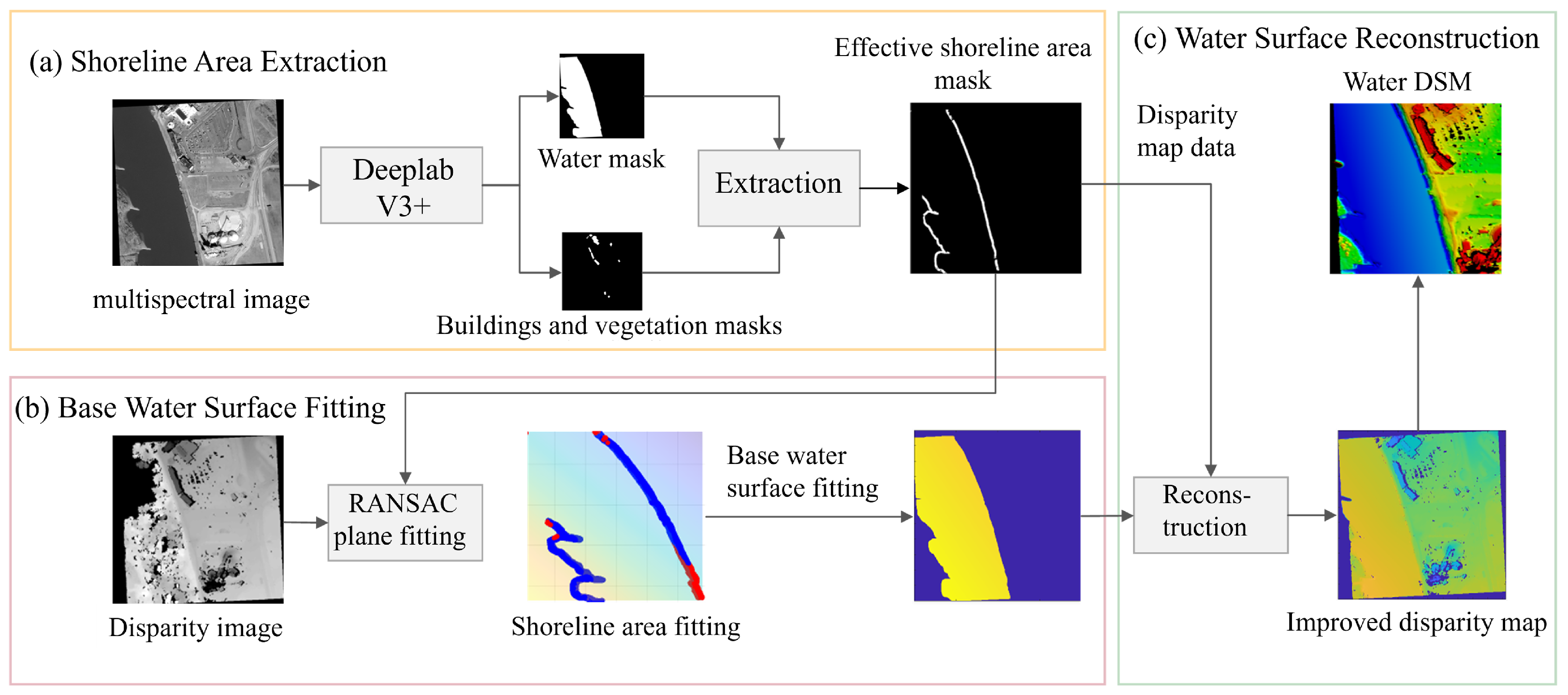
The overall framework of our algorithm is demonstrated in Figure 1. The algorithm comprises the following three parts, and the time complexity of our algorithm is , where n represents the number of pixels in the disparity image of the target water region:
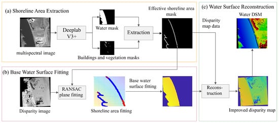
Figure 1.
Overall framework of our algorithm: (a) Effective shoreline area extraction: The multispectral image includes the R, G, and B bands, which are useful to semantic segmentation. Multiple strategies are employed to derive an effective shoreline ground mask. (b) Base water surface fitting: On the basis of the effective shoreline data, a RANSAC plane fitting strategy with slope and inclination constraints is applied to assign values to the water surface region according to the fitted plane parameters, resulting in a base water surface. “Disparity image” is generated by SGM [22] (c) Seamless water surface reconstruction: A high-precision water surface DSM is generated on the basis of the optimized disparity map.
- Effective shoreline area extraction: this article uses the DeepLabV3+ [18] pretrained model to extract water surfaces, buildings, and vegetation masks from multispectral satellite imagery corresponding to the target locations. After morphological processing, an initial shoreline area is obtained. Multiple strategies are employed to derive an effective shoreline ground mask.
- Base water surface fitting: On the basis of the effective shoreline data, a RANSAC [35] plane fitting strategy with slope and inclination constraints is applied to assign values to the water surface region according to the fitted plane parameters, resulting in a base water surface. The original disparity image is generated by SGM [22]. The time complexity of this part is , where n denotes the number of pixels in the disparity image of the target water region. This complexity arises because, after the plane is fitted using a small set of control points (whose number is negligible relative to n), each pixel within the target water region is assigned a disparity value based on a simple planar equation. This per-pixel assignment requires constant time, leading to a total linear complexity with respect to the number of pixels.
- Seamless water surface reconstruction: Starting with the base water surface as the initial value, a second-order smoothing water surface reconstruction model is established to obtain a seamlessly connected disparity-optimized result. A high-precision water surface DSM is generated on the basis of the optimized disparity image. This part achieves linear time complexity , with n representing the pixel count in the water region’s disparity image. The linear complexity arises because the reconstruction model operates directly on each pixel in the disparity map using local neighborhood information (e.g., second-order derivatives or convolutional filters). These operations involve a fixed number of computations per pixel, resulting in a total processing time that scales linearly with the number of pixels in the target region.
3.1. Shoreline Area Extraction
3.1.1. Water, Vegetation, and Building Mask Extraction
This article uses the DeepLabV3+ neural network [18] to perform semantic segmentation on satellite stereo imagery, obtaining masks for water bodies, vegetation, and building areas. Segmentation is conducted using pretrained models from OpenMMlab on the LoveDA [36] dataset. To validate the accuracy of water body extraction, experiments were conducted on test data and compared with manually drawn water body areas, achieving an accuracy of 96%, an Intersection over Union (IoU) score of 0.88, and an F1 score of 0.94. Given the distinctiveness of water body features and the high accuracy, the extraction of water body regions is considered reliable and provides a foundation for subsequent water surface DSM optimization work without manual editing. However, since the LoveDA [36] dataset was not specifically designed for water mask extraction, the generalization capability of its pretrained models for water body segmentation across other satellite imagery requires further validation.
3.1.2. Effective Shoreline Area Extraction
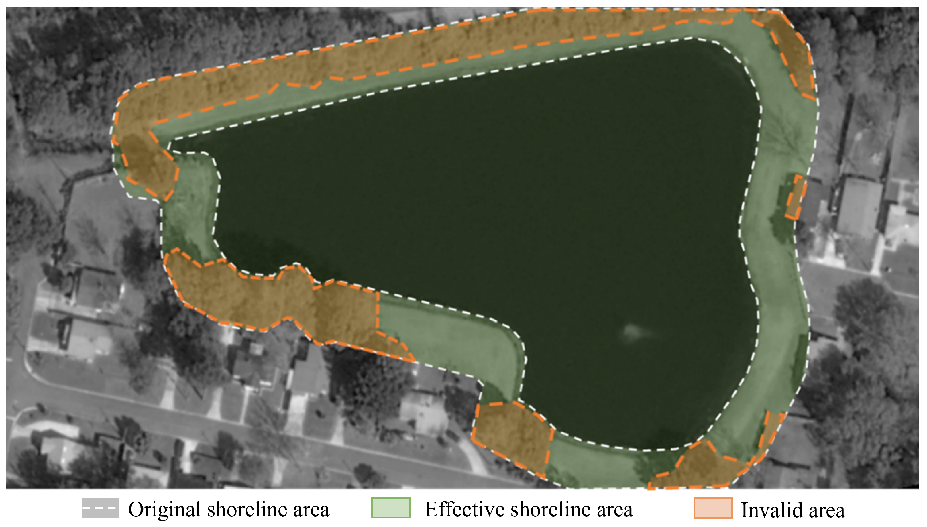
To extract the effective shoreline area, this article first performs dilation in morphological processing to expand the connected water body regions and obtain preliminary shoreline areas by subtracting these areas from the original region. Then, vegetation and building masks are applied to filter the shoreline areas, retaining only the shoreline ground regions. This step reduces the impact of abnormal elevations from vegetation and buildings on water surface plane fitting, addressing the issue of water surface overestimation. Figure 2 shows the effective shoreline area extraction under ideal conditions. The white dashed line represents the extracted preliminary shoreline area, with the orange region indicating the excluded invalid areas and the green region denoting the retained effective shoreline area. Given that the extraction accuracy of vegetation or building masks may be limited and considering the smoothing characteristics of actual shoreline ground region disparity, slope and inclination thresholds for regional disparity are set to eliminate outliers.
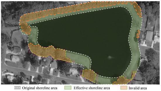
Figure 2.
Effective shoreline area extraction under ideal conditions. The white dashed line represents the extracted preliminary shoreline area, the orange region indicates the excluded invalid areas, and the green region denotes the retained effective shoreline area.
3.2. Base Water Surface Fitting
The original disparity image in Figure 1b is generated by SGM [22]. Given the approximately planar nature of water surfaces and their comparable elevation to adjacent shorelines, this article fully utilizes the effective shoreline area. For each water body connectivity region, the effective shoreline area is fitted to a plane to calculate the plane fitting parameters of the water body region. Considering that there may still be some outliers in the effective shoreline area, the RANSAC algorithm [35] is employed to robustly estimate the plane equation parameters of the water body. Additionally, since the inclination angle of the water surface plane is relatively small, inequality constraints are further set to limit the inclination angle of the fitting plane. The fitting of the effective shoreline plane area is achieved by solving the following minimization problem:
where n represents the number of points in the valid shoreline area; , , and represent the coordinates of each point; and a, b, and c are the parameters of the fitted plane.
In addition, the model mentioned above is subject to the following conditions to prevent excessive tilt during the plane-fitting process:
where represents the preset angle threshold for the plane inclination. This constraint ensures that the fitted plane will not be overly inclined. Through deduction, it is determined that the angle threshold equals 1°. The deduction process is as follows.
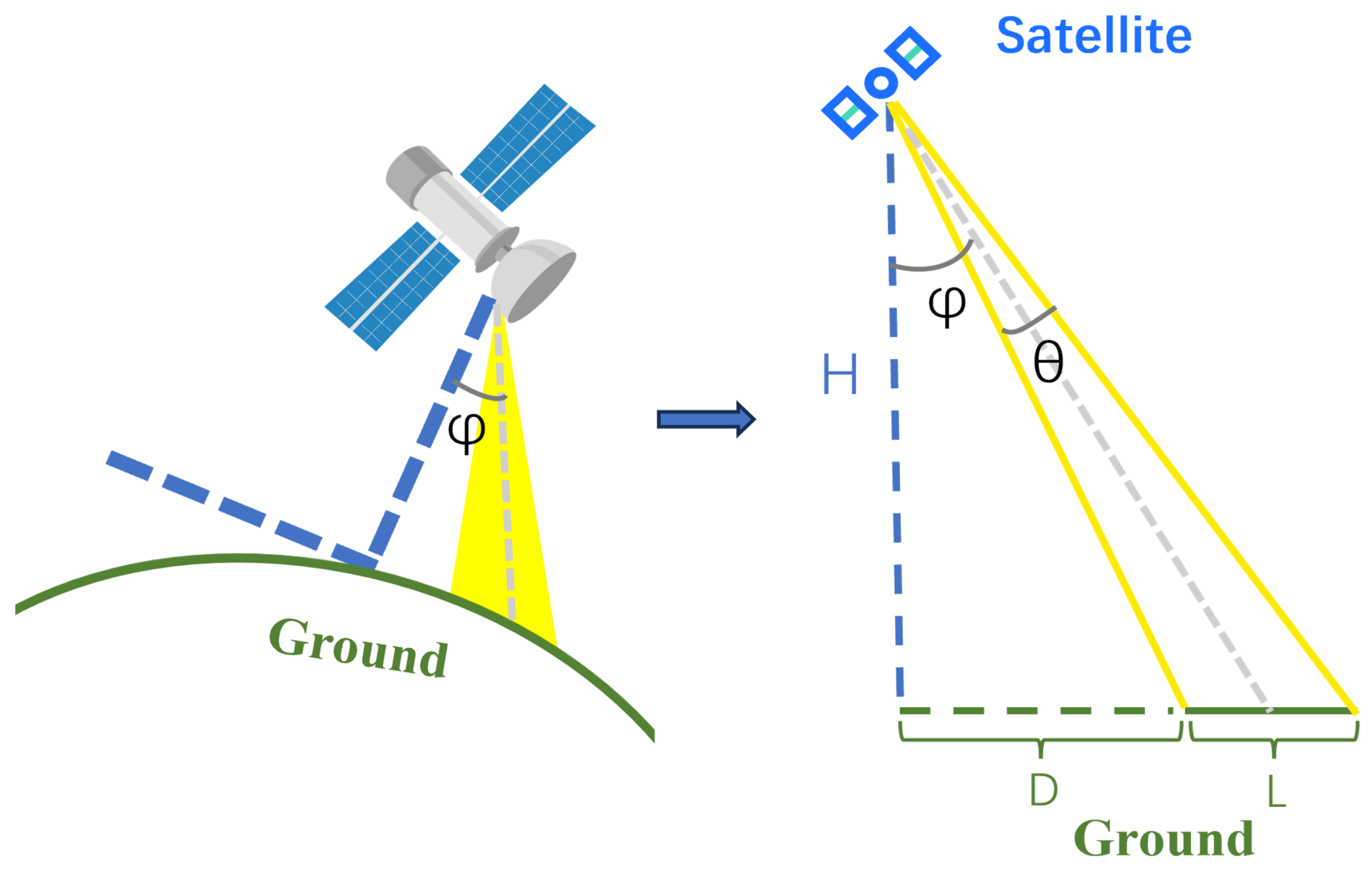
We can see from Figure 3 that
where H denotes the satellite’s orbital altitude, D represents the horizontal distance, and L refers to a line segment within the ground imaging plane. The maximum value of L is used for simplicity. is the off-nadir angle or backward angle, and is the angle formed by the light entering the satellite camera. It can be observed that L is roughly the same. As the angle increases, the depth variation between the near and far points becomes more pronounced, and the value in disparity also increases accordingly, leading to a greater inclination angle of the fitted reference plane. By calculating the first-order derivative of the right side of Equation (4) with respect to , it can be determined that, when reaches its minimum value of 5°, reaches its maximum value of 0.6°. When is sufficiently small, can be approximated as the slope of the fitted water surface. After rounding, is set to 1° as the threshold constraint for the plane slope. While satellite imaging inevitably introduces tilt angles that vary across regions, our boundary constraints demonstrate robust adaptability to diverse geographical conditions. The specific parameter values automatically adjust according to sensor characteristics and image dimensions, ensuring consistent performance.
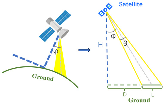
Figure 3.
Angle threshold deduction process. The left side represents a schematic diagram of the satellite’s flight process, whereas the right side shows a planar diagram for easier calculation. H denotes the satellite’s orbital altitude, D represents the horizontal distance, and L refers to a line segment within the ground imaging plane. For simplicity in the calculations, the maximum value of L is used, corresponding to the ground length of the image diagonal. is the off-nadir angle or backward angle, and is the angle formed by the light entering the satellite camera during the imaging process.
In this work, the RANSAC algorithm [35] is used to enforce the angle constraint during plane fitting. Finally, by assigning values to the corresponding connected regions of the water surface, the initial values for the water surface to be reconstructed are obtained.
Our algorithm can perform individual plane fitting for each connected water region. However, certain special cases may lead to an insufficient number of pixels in valid coastal areas, such as water bodies with bridges on one side or lakes surrounded by trees, as shown in Figure 4. Therefore, this article proposes a “global plane fitting” strategy; when there is a lack of effective shoreline areas, our algorithm automatically identifies and applies integrated plane fitting to all connected water regions. For regions with insufficient effective shoreline areas, the inner boundaries are assigned the parameters of the globally fitted plane, and the corresponding base water surface is also assigned the global plane parameters.
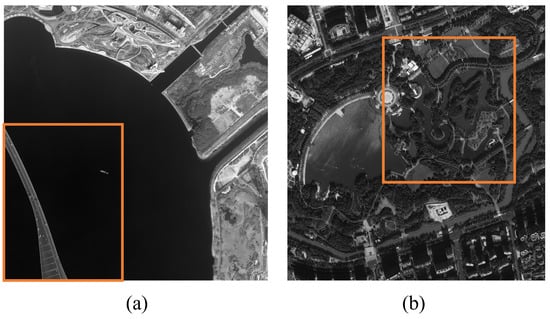
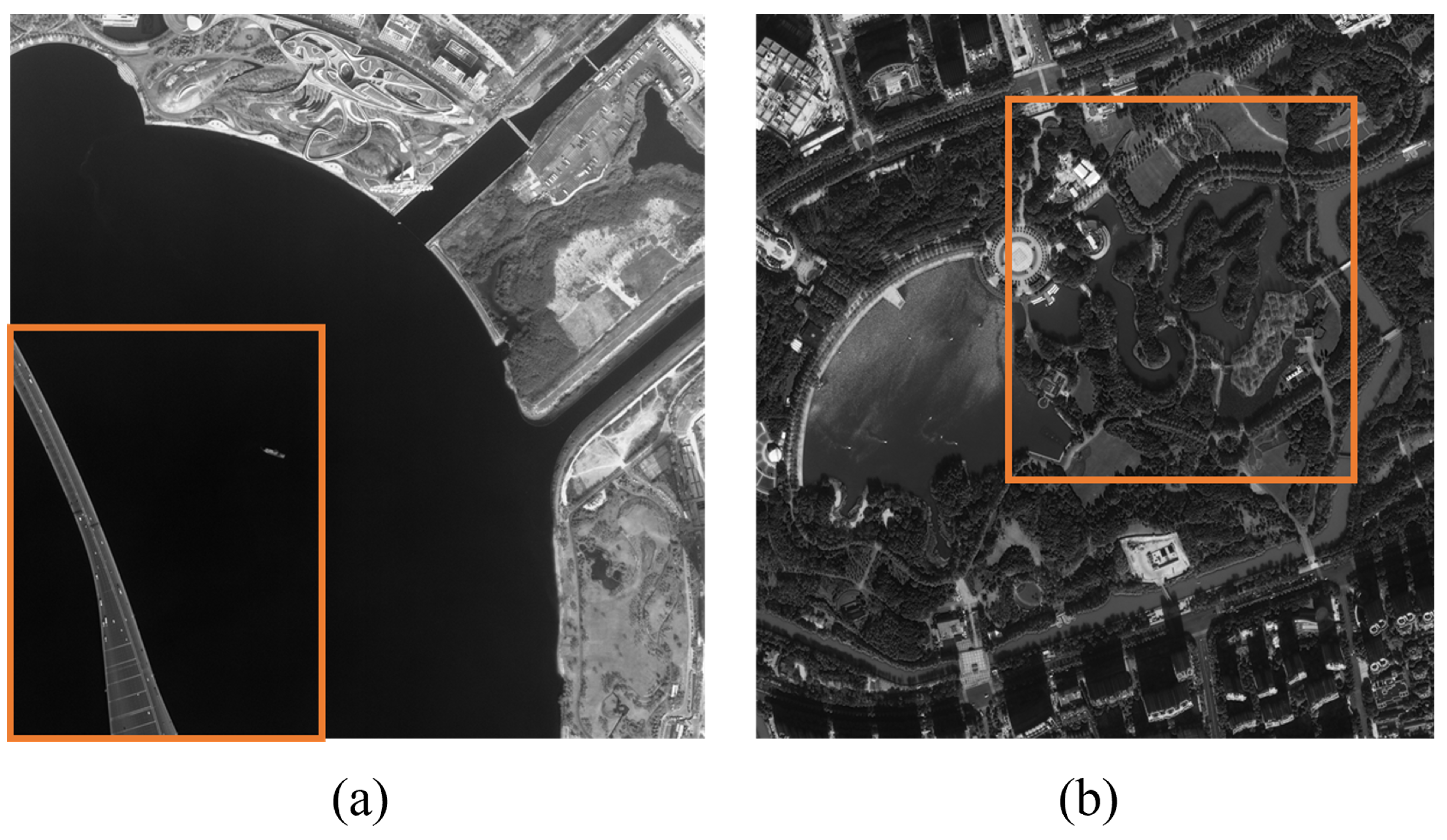
Figure 4.
The orange box contains examples of special cases: (a) water bodies with a bridge on one side and (b) lakes surrounded by trees.
3.3. Seamless Water Surface Reconstruction
Directly applying the base water surface obtained from plane fitting can lead to noticeable seams between the water surface and the shoreline. To achieve a smooth transition between the water surface and the shoreline, the proposed disparity optimization follows the principle of Poisson blending [37], enforcing gradient field preservation and boundary consistency to achieve seamless reconstruction across weak texture regions, applying plane conditions and boundary conditions in a reasonable manner, namely maintaining consistent disparity at the interface between the water surface and the shoreline to eliminate linear artifacts. The preliminary model is given below:
where represents the optimized disparity value for the water surface area, I represents the disparity value of the unoptimized region, x and y represent the plane coordinates, represents the water surface area, represents the boundary of the water surface area, ∇ represents the Laplace operator, and E represents the constructed energy function, with the goal of minimizing this energy function. Experimental validation confirms the boundary constraints’ effectiveness in different water bodies, including river, lake, and sea. The algorithm maintains stability despite variations in water surface characteristics and surrounding terrain.
In this model, the plane constraint is represented by a zero second-order gradient, reflecting that the calm water surface under normal conditions closely approximates a planar geometry. When the second-order gradient of a region is zero, the image within that region is smooth, without edges or textures, which is equivalent to a plane. At the same time, the condition for seamless boundary connection is retained, meaning that the values in the boundary region remain unchanged. This is then combined with the results of plane fitting under the plane angle constraint to ensure that the final water surface area result avoids excessive plane tilt and seamlessly connects with the shoreline.
For the water bodies at the edges of the images, our proposed algorithm automatically uses the shoreline fitting plane parameters corresponding to the individual connected water regions to assign values to the image edge areas, constructing a “virtual shoreline” to prevent the excessive warping of the plane from single-sided effects. This article assigns the disparity values from whole effective shoreline areas in the image to water regions at the image edges. In summary, by optimizing the water surface area in the disparity map through water surface reconstruction, the reconstructed water body area DSM is effectively optimized.
4. Experiments
4.1. Datasets
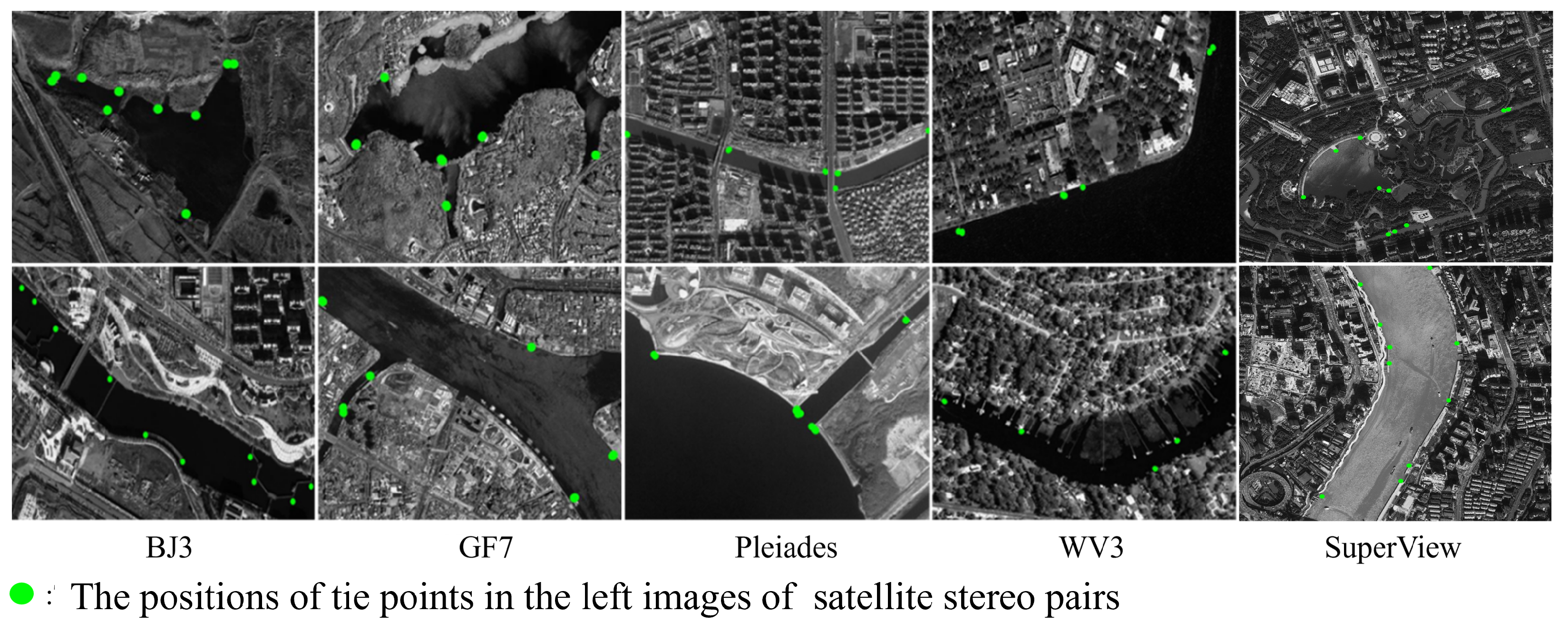
In our experiment, 10 high-resolution satellite stereo image pairs are used to verify the effectiveness of our algorithm. The satellite images were acquired under conditions absent of both wave activity and ice coverage. While wave activity and ice coverage may degrade water surface DSM reconstruction in other methods mentioned in this article, our algorithm remains unaffected by these disturbances. Compared to conventional optical satellite imagery, this dataset offers superior resolution and provides same-orbit stereo pairs, making it particularly suitable for high-accuracy dense matching applications. It includes Beijing-3 images with 0.3 m spatial resolution from Taian City, Shandong Province; GaoFen-7 (GF-7) images with 0.65 m spatial resolution from Guangzhou City, Guangdong Province; Pleiades images with 0.5 m spatial resolution from Shanghai and Shenzhen; Superview images with 0.5 m spatial resolution from Shanghai, China; and WorldView-3 (WV-3) images with 0.3 m spatial resolution from Jacksonville, FL, USA. As shown in Figure 5, the satellite images cover common water body types such as lakes, rivers, and seas, making them representative for water area reconstruction. Meanwhile, multispectral satellite images of the same regions are also utilized for effective shoreline area extraction. In the following section, we primarily introduce the use of panchromatic stereo satellite imagery for image dense matching.
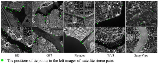
Figure 5.
For each high-resolution satellite stereo pair, the left-view image is presented. Tie points are selected from effective shoreline area near each connected water body region, and the distribution of tie points is marked with green circles. The extraction of tie points is influenced by key imaging parameters, including resolution, viewing geometry, scene extent, and noise characteristics, which collectively determine both the quantity and matching reliability.
4.1.1. Beijing-3 Images
We use Beijing-3B’s panchromatic images of 0.3 m spatial resolution from a lake and a river in Taian City, Shandong Province. The pixel sizes of the two types of images are 3087 × 3193 and 3086 × 3193. The satellite’s off-nadir angle and orbital altitude are 53° and 620 km [38], respectively. The data in Figure 5 shows that there are buildings, vegetation, and bridges near the water body in the Beijing-3 images; for these areas, multiple strategies are used to cull them.
4.1.2. GF-7 Images
We use GF-7 images with 0.65 m resolution from a lake and a river in Guangzhou City, Guangdong Province. The pixel sizes of the two types of images are 3579 × 3490 and 3558 × 3486. The satellite’s backward angle and orbital altitude are 5° and 645 km [39], respectively.
4.1.3. Pleiades Images
We use Pleiades panchromatic images of 0.5 m spatial resolution from a river in Shanghai and sea near Shenzhen. The pixel sizes of the two types of images are 2766 × 2895 and 3029 × 3092. The satellite’s off-nadir angle and orbital altitude are 47° and 694 km [40].
4.1.4. SuperView Images
We use SuperView images with 0.5 m resolution from a river and a lake in Shanghai City. The pixel sizes of the two types of images are 3871 × 4386 and 3704 × 4316. The satellite operates at an orbital altitude of approximately 530 km, with an off-nadir angle ranging between 6° and 10° [41].
4.1.5. WV-3 Images
We use WV-3 panchromatic images from a river and sea in Jacksonville, FL, USA. The pixel sizes of the two types of images are 2993 × 3070 and 3013 × 3072. The satellite’s off-nadir angle and orbital altitude are 70° and 617 km [42].
4.2. Implementation and Evaluation Metrics
4.2.1. Implementation Details
To assess the accuracy of the water body area reconstruction, tie points are selected from effective shoreline areas near each connected water body region in satellite stereo pairs due to the lack of reliable tie points on the water surfaces, and obtain their elevations via forward intersection. To better fit the ground truth data, the tie points must be extracted from the shoreline–water interface where distinctive matching features exist and the results show that the number of tie points selected is enough. Given the fact that the elevation of the shoreline regions closely approximates water surface elevation, the water surface elevation is determined by fitting a plane to discrete data points for accuracy validation. As shown in Figure 5, the distribution of tie points is marked with green circles.
To validate accuracy, this study compares the DSMs generated by SGM [22], DSMs generated by ACVNet [14], GwcNet [43], HFF [44], PSMNet [45], ASF [46], and IGEV++ [13] with high-precision registration, the DSMs generated by Reconstruction Master version 6.0 [34], and the DSMs generated by the proposed BPC-SWSR.
4.2.2. Evaluation Metrics
To evaluate the performance of the proposed method, this article first manually obtains the masks of the water regions, then three common metrics are used: the root mean square error (RMSE) in water surface region, the mean error (ME) in water surface region, and the variance (VAR) in water surface region. The first two metrics assess the accuracy of the reconstruction results, and VAR is calculated to assess the smoothness of the water surface reconstruction. On the basis of the fitted truth plane above, the DSM results and the manually delineated water mask, the RMSE is calculated via the following formula:
where n represents the number of pixels in the water mask, represents the observed evaluation, and represents the true evaluation in the DSM. The ME is derived using the following equation:
where n represents the number of pixels in the water mask, represents the observed evaluation, and represents the true evaluation in the DSM. The VAR is calculated via the following formula:
where n represents the number of pixels in the water mask, represents the observed evaluation, and represents the mean of the observed evaluation in the water mask.
4.3. Comparison with Other Methods
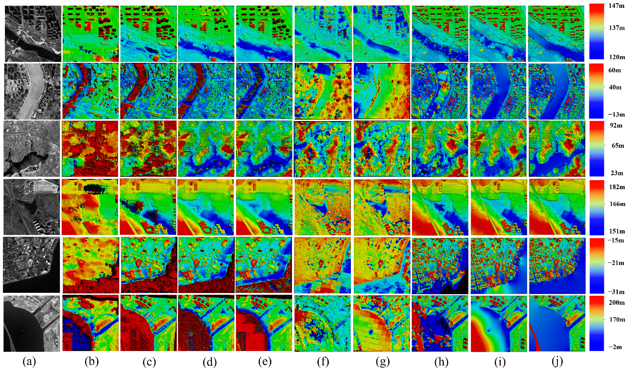
The proposed BPC-SWSR is compared with our baseline SGM [22] and several existing advanced algorithms, including Reconstruction Master version 6.0 [34], ACVNet [14], GwcNet [43], HFF [44], PSMNet [45], ASF [46], and IGEV++ [13]. All comparative methods were configured with their current state-of-the-art default parameters to ensure fair benchmarking. Figure 6 shows the DSMs generated by different algorithms, demonstrating the superiority of the reconstruction results of the proposed algorithm. Table 1 quantifies the results presented in Figure 6 by calculating three metrics. The performance of the first four methods is notably poor in sea environments, whereas our algorithm exhibits strong universality across various water bodies.
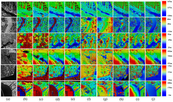
Figure 6.
DSMs generated by different algorithms. (a) Image. The first row and the fourth row are Beijing-3 images, the second row is Superview image, the third row is a GF-7 image, the fifth row is a WV-3 image, and the third row is a Pleiades image. (b) ACVNet [14]. (c) GwcNet [43]. (d) HFF [44]. (e) PSMNet [45]. (f) ASF [46]. (g) IGEV++ [13]. (h) SGM [22]. (i) Reconstruction Master version 6.0 [34]. (j) Ours. Our proposed BPC-SWSR has superior performance in water surface optimization.

Table 1.
Comparison of DSM in different methods.
4.3.1. Quantitative Comparison
To validate the accuracy of our results, tie points are manually selected in satellite stereo pairs for plane fitting, assume that it is the real water surface, and then calculate the RMSE, ME, and VAR of the reconstruction results under different methods in turn. As shown in Table 1, the results generated by the proposed BPC-SWSR show improvements in accuracy and smoothness compared with the results of the commercial software Reconstruction Master version 6.0 [34], and the results of this algorithm are the best in each set of test data.
The RMSE of the method proposed in this article is within 4 m. The mean RMSE of our method is 2.279 m, which is significantly lower than the average RMSE of 229.2 m achieved by the other methods. The ME of our method is within 3 m, with a mean ME of 1.971 m, which is significantly lower than the mean ME of 223.8 m for the other methods. The VAR of our method is within 1.5 m2, with a mean VAR of 0.6613 m2, which is significantly lower than the mean VAR of 522.5 m2 for existing methods.
Moreover, the four methods, namely ACVNet [14], GWC [43], HFF [44], and PSM [45], show a notably suboptimal performance in the context of sea environments. With the exception of the Reconstruction Master version 6.0 [34] and our proposed method, all the other methodologies exhibit a progressive decline in efficacy when transitioning from river to lake to sea scenarios. This trend can be attributed to the increasing difficulty in identifying effective tie points as the water body increases.
4.3.2. Qualitative Comparison
The DSMs generated by different algorithms are shown in Figure 6. The reconstruction outcomes of ACVNet [14] and GWC [43] scarcely reveal the characteristics of water bodies. HFF [44] and PSM [45] yield relatively favorable results at the margins of rivers and lakes; however, their reconstructions are marred by a significant prevalence of invalid values and voids at the center, with the proportion of such anomalies reaching their zenith in sea environments. The SGM [22] reconstruction is beset by numerous anomalous undulations in rivers and lakes due to the influence of shorelines and is further compromised by extensive voids in the sea. The Reconstruction Master version 6.0 [34], while second only to our method, results in protrusions at the juncture of shorelines and is most severely impacted by edge effects in the sea.
The data in Figure 6 shows that, among the 8 methods compared with our method, the reconstruction effectiveness in the sea, which represents a large-scale water body, is significantly inferior to that in rivers and lakes, which are smaller in scale. In contrast, our algorithm, which is distinguished by its “virtual shoreline” strategy, demonstrates remarkable adaptability across water bodies of varying sizes.
5. Discussion
5.1. Effect of Removing Shoreline Vegetation and Buildings Areas
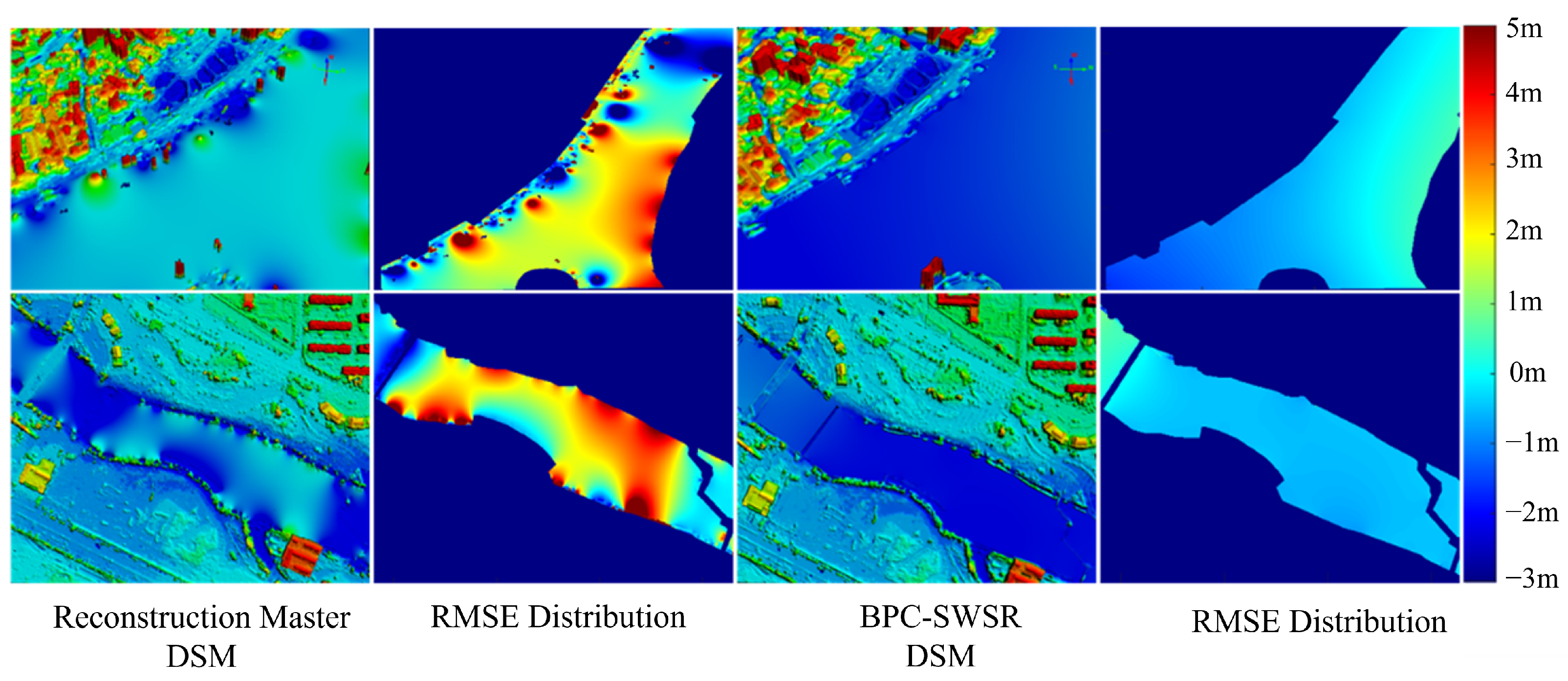
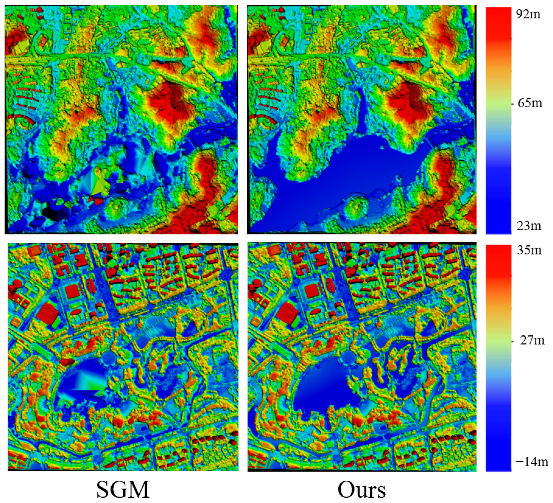
To evaluate the effects of removing shoreline vegetation and building areas, this article compares the experimental data obtained via direct water surface fitting with those obtained via water surface fitting after boundary filtering, which involves removing ineffective shoreline areas prior to fitting. As seen in the second and third rows of Table 2, the RMSE decreased to 1/3 of its original value after applying boundary filtering, whereas the variance decreased to 1/4 of its original value. Moreover, by drawing RMSE distribution maps generated by Reconstruction Master version 6.0 [34] and the proposed BPC-SWSR, which can be seen in Figure 7, we find that Reconstruction Master version 6.0 [34] will create trees or buildings and the water surface abnormally connected in the shore area, resulting in abnormal water surface undulations. However, the optimization algorithm in this study does not cause the water surface to be abnormally higher than the ground because we use masks to exclude interference from shore vegetation and building elevations when extracting the effective shoreline area.
Table 2.
Ablation study.
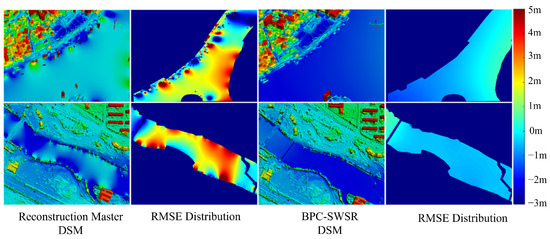
Figure 7.
DSM results and RMSE distribution maps generated by the Reconstruction Master version 6.0 [34] and the proposed BPC-SWSR. The second column is generated by Reconstruction Master version 6.0 [34] and the fourth column is generated by ours. The first row shows the reconstruction results from the GF-7 images. The second row shows the reconstruction results from the Beijing-3 images. Reconstruction Master version 6.0 [34] makes trees or buildings and the water surface abnormally connected in the shore area, resulting in abnormal water surface undulations.
5.2. Effect of Seamless Water Surface Reconstruction
The algorithm uses the idea of Poisson blending [37] to achieve seamless water surface reconstruction. We can see in the third and fourth rows of Table 2 that, with Poisson blending, the RMSE and variance are reduced by 2.1%, and the mean error is decreased by 3.6%.
5.3. Influence of the Global Plane Fitting Strategy
The data in Figure 8 show that the DSM results generated by SGM [22] contain many anomalous undulations in the lakes surrounded by vegetation and buildings. Moreover, selecting effective shoreline areas for these lakes is challenging. Our proposed “global plane fitting” strategy ensures that the reconstruction results are not affected by vegetation and buildings, preventing anomalous undulations.
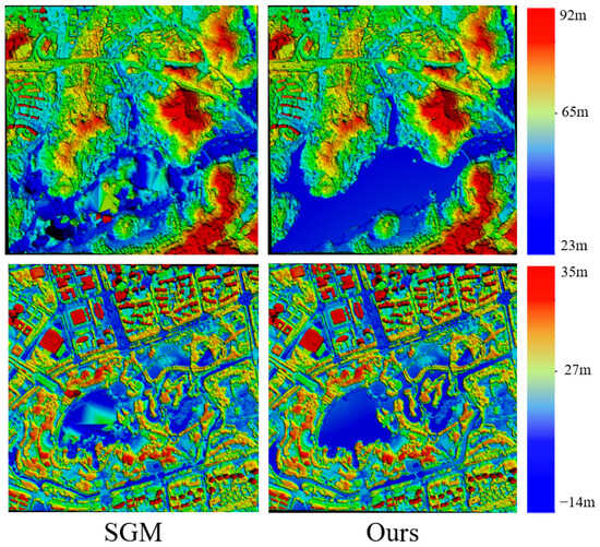
Figure 8.
The reconstruction results of SGM [22] and our algorithm for lakes with shorelines predominantly covered by vegetation and buildings.
5.4. Influence of the Virtual Shoreline Strategy
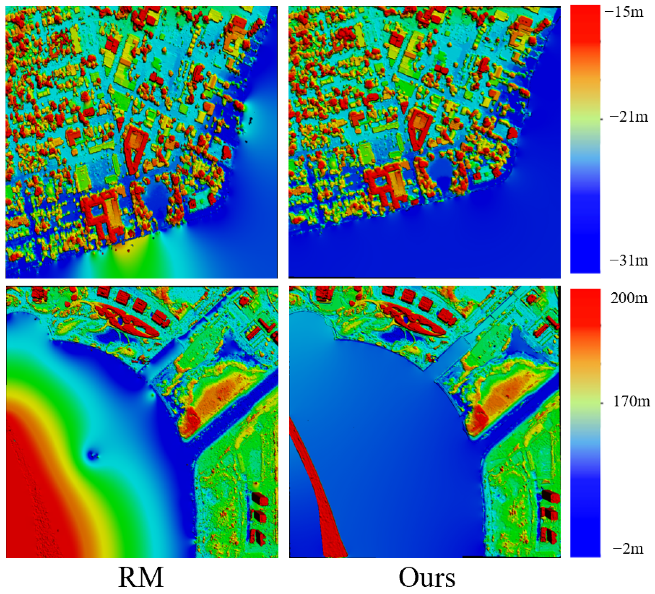
As shown in Figure 9, due to the large water surface area, finding effective tie points is challenging, leading to inflated readings and the excessive warping of the plane from single-sided effects in the results of Reconstruction Master version 6.0 [34]. In contrast, the “virtual shoreline” strategy in our approach enhances the accuracy and smoothness of the reconstruction results on the sea.
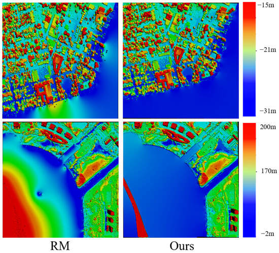
Figure 9.
The reconstruction results of Reconstruction Master version 6.0 [34] and our algorithm in large-scale sea environments.
5.5. Advantages and Limitation Analysis
Compared to satellite altimetry’s along-track observations with inherent spatial sparsity, our stereo-image-based approach generates continuous and high-resolution water surface elevation models. While optical data alone lacks three-dimensional information, our BPC-SWSR method effectively bridges this gap through constrained stereo reconstruction, enabling comprehensive water surface modeling at landscape scales. However, there are still limitations in our algorithm. First, the accuracy of extracting effective water bodies and shoreline areas needs to be improved, as this affects the reconstruction results. Second, although the assumption is that the entire water body area is poorly matched, there may actually be some correctly matched information. Fully utilizing this information may lead to a better results. Thirdly, the water surface DSMs generated by our algorithm remain stable because they are based on the effective shoreline area. However, in real-world conditions, water surfaces are often dynamic due to waves or currents, which may introduce variability not fully captured in the current model.
6. Conclusions
In this work, this article proposes a water surface stereo reconstruction algorithm based on boundary plane constraints that uses effective shoreline tie points to optimize the reconstruction of weak texture regions, resulting in smoother and more accurate water surface reconstructions. Through plane and tilt angle constraints, the seamless planar reconstruction of water areas is achieved, effectively addressing common issues in past reconstruction, such as voids, irregular gaps, and abnormal undulations. The proposed method demonstrates superior performance in estimating water surface elevation, achieving a mean RMSE of 2.279 m, which is significantly lower than the average RMSE of 229.2 m obtained by existing methods. Similarly, the mean ME of our method is 1.971 m, compared to 223.8 m for other approaches. In terms of variance, our method also outperforms others, with a mean VAR of 0.6613 m2, substantially lower than the 522.5 m2 reported by other state-of-the-art methods. However, abnormal undulations exist in the DSMs generated by existing methods. If they are not invalid values, they will be included in the metric evaluations. This may be one of the reasons why all three metrics of the existing methods are relatively high. In the meanwhile, there is still room for improvement in water surface reconstruction work. This study utilizes only panchromatic imagery. Future work could consider combining with shoreline and other ancillary data sources and we will explore more methods to increase the accuracy and efficiency of water surface reconstruction.
Author Contributions
Conceptualization, X.H.; methodology, J.Y. and X.H.; software, J.Y. and R.X.; validation, J.Y. and R.X.; formal analysis, R.X.; investigation, J.Y. and R.X.; resources, X.H.; data curation, R.X.; writing—original draft preparation, J.Y. and R.X.; writing—review and editing, R.X. and Y.W.; visualization, R.X.; supervision, X.H. All authors have read and agreed to the published version of the manuscript.
Funding
This research was funded by Fundamental Research Funds for the Central Universities, Sun Yat-sen University (grant number 24xkjc002).
Institutional Review Board Statement
Not applicable.
Informed Consent Statement
Not applicable.
Data Availability Statement
The satellite images used in this study, including those from Beijing-3, GF-7, Pleiades, SuperView, and WV-3, were obtained from commercial or restricted sources and are not publicly available due to licensing constraints. No new publicly shareable datasets were generated in this study.
Acknowledgments
The authors gratefully acknowledge the use of Reconstruction Master version 6.0 software for digital surface model generation. We also thank the providers of satellite imagery, including Beijing-3, GF-7, Pleiades, SuperView, and WV-3, for supporting the experiments conducted in this study. During the preparation of this manuscript, the authors used DeepSeekto assist with phrasing suggestions. The authors have reviewed and edited the output and take full responsibility for the content of this publication.
Conflicts of Interest
The authors declare no conflicts of interest.
Abbreviations
The following abbreviations are used in this manuscript:
| BPC-SWSR | boundary plane-constrained surface water stereo reconstruction |
| RM | Reconstruction Master version 6.0 |
| RMSE | Root mean squared error |
| ME | Mean error |
| VAR | Variance |
| DSM | Digital surface model |
References
- El Garouani, A.; Alobeid, A.; El Garouani, S. Digital surface model based on aerial image stereo pairs for 3D building. Int. J. Sustain. Built Environ. 2014, 3, 119–126. [Google Scholar] [CrossRef]
- Guerin, C.; Binet, R.; Pierrot-Deseilligny, M. Automatic Detection of Elevation Changes by Differential DSM Analysis: Application to Urban Areas. IEEE J. Sel. Top. Appl. Earth Obs. Remote Sens. 2014, 7, 4020–4037. [Google Scholar] [CrossRef]
- Zhou, Q. Digital elevation model and digital surface model. Int. Encycl. Geogr. People Earth Environ. Technol. 2017, 1–17. [Google Scholar] [CrossRef]
- Yuan, X.; Tian, J.; Reinartz, P. A Self-Training Approach Using Benchmark Dataset and Stereo-DSM for Building Extraction. IEEE J. Sel. Top. Appl. Earth Obs. Remote Sens. 2024, 17, 11352–11364. [Google Scholar] [CrossRef]
- Brunn, A.; Weidner, U. Extracting buildings from digital surface models. Int. Arch. Photogramm. Remote Sens. 1997, 32, 27–34. [Google Scholar]
- Altmaier, A.; Kany, C. Digital surface model generation from CORONA satellite images. ISPRS J. Photogramm. Remote Sens. 2002, 56, 221–235. [Google Scholar] [CrossRef]
- White, J.C.; Wulder, M.A.; Vastaranta, M.; Coops, N.C.; Pitt, D.; Woods, M. The utility of image-based point clouds for forest inventory: A comparison with airborne laser scanning. Forests 2013, 4, 518–536. [Google Scholar] [CrossRef]
- Zhang, L. Automatic Digital Surface Model (DSM) Generation from Linear Array Images; ETH: Zurich, Switzerland, 2005. [Google Scholar]
- Zheng, Y.; Yang, S.; Li, Y.; Wu, J.; Shi, Z.; Kou, R. A Heterogeneous Remote Sensing Image Matching Method for Urban Areas with Complex Terrain Based on 3D Spatial Relationship Constraints. IEEE J. Sel. Top. Appl. Earth Obs. Remote Sens. 2024, 17, 6791–6804. [Google Scholar] [CrossRef]
- Adhyapak, S.A.; Kehtarnavaz, N.; Nadin, M. Stereo matching via selective multiple windows. J. Electron. Imaging 2007, 16, 013012. [Google Scholar] [CrossRef]
- Huang, X.; Zhang, Y.; Yue, Z. Image-guided non-local dense matching with three-steps optimization. ISPRS Ann. Photogramm. Remote Sens. Spat. Inf. Sci. 2016, 3, 67–74. [Google Scholar]
- Wu, B.; Zhang, Y.; Zhu, Q. A triangulation-based hierarchical image matching method for wide-baseline images. Photogramm. Eng. Remote Sens. 2011, 77, 695–708. [Google Scholar] [CrossRef]
- Xu, G.; Wang, X.; Zhang, Z.; Cheng, J.; Liao, C.; Yang, X. IGEV++: Iterative Multi-range Geometry Encoding Volumes for Stereo Matching. IEEE Trans. Pattern Anal. Mach. Intell. 2025, 1–15. [Google Scholar] [CrossRef]
- Xu, G.; Cheng, J.; Guo, P.; Yang, X. Attention concatenation volume for accurate and efficient stereo matching. In Proceedings of the IEEE/CVF Conference on Computer Vision and Pattern Recognition, New Orleans, LA, USA, 18–24 June 2022; pp. 12981–12990. [Google Scholar]
- Chen, K.; Chen, B.; Liu, C.; Li, W.; Zou, Z.; Shi, Z. Rsmamba: Remote sensing image classification with state space model. IEEE Geosci. Remote Sens. Lett. 2024, 21, 8002605. [Google Scholar] [CrossRef]
- Zheng, S.; Lu, C.; Wu, Y.; Gupta, G. SAPNet: Segmentation-aware progressive network for perceptual contrastive deraining. In Proceedings of the IEEE/CVF Winter Conference on Applications of Computer Vision, Waikoloa, HI, USA, 3–8 January 2022; pp. 52–62. [Google Scholar]
- Li, X.; Xu, F.; Liu, F.; Tong, Y.; Lyu, X.; Zhou, J. Semantic segmentation of remote sensing images by interactive representation refinement and geometric prior-guided inference. IEEE Trans. Geosci. Remote Sens. 2023, 62, 5400318. [Google Scholar] [CrossRef]
- Chen, L.C.; Zhu, Y.; Papandreou, G.; Schroff, F.; Adam, H. Encoder-decoder with atrous separable convolution for semantic image segmentation. In Proceedings of the European Conference on Computer Vision (ECCV), Munich, Germany, 8–14 September 2018; pp. 801–818. [Google Scholar]
- Scharstein, D.; Szeliski, R. A taxonomy and evaluation of dense two-frame stereo correspondence algorithms. Int. J. Comput. Vis. 2002, 47, 7–42. [Google Scholar] [CrossRef]
- Sha, H.; Yuan, X. The Review and Prospect of Dense Matching Methods for Stereo Imagery. Geomat. Inf. Sci. Wuhan Univ. 2023, 48, 1813–1833. [Google Scholar]
- Zhu, C.T.; Chang, Y.Z.; Wang, H.M.; He, K.; Lee, S.T.; Lee, C.F. Efficient stereo matching with decoupled dissimilarity measure using successive weighted summation. Math. Probl. Eng. 2014, 2014, 127284. [Google Scholar] [CrossRef]
- Huang, X.; Han, Y.; Hu, K. An improved semi-global matching method with optimized matching aggregation constraint. In IOP Conference Series: Earth and Environmental Science; IOP Publishing: Bristol, UK, 2020; Volume 569, p. 012050. [Google Scholar]
- Xiang, J.; Li, Z.; Kim, H.S.; Chakrabarti, C. Hardware-efficient neighbor-guided SGM optical flow for low power vision applications. In Proceedings of the 2016 IEEE International Workshop on Signal Processing Systems (SiPS), Dallas, TX, USA, 26–28 October 2016; IEEE: Piscataway, NJ, USA, 2016; pp. 1–6. [Google Scholar]
- Hirschmüller, H.; Buder, M.; Ernst, I. Memory efficient semi-global matching. ISPRS Ann. Photogramm. Remote Sens. Spat. Inf. Sci. 2012, 1, 371–376. [Google Scholar] [CrossRef]
- Kanade, T.; Okutomi, M. A stereo matching algorithm with an adaptive window: Theory and experiment. IEEE Trans. Pattern Anal. Mach. Intell. 1994, 16, 920–932. [Google Scholar] [CrossRef]
- Zhang, K.; Lu, J.; Lafruit, G. Cross-based local stereo matching using orthogonal integral images. IEEE Trans. Circuits Syst. Video Technol. 2009, 19, 1073–1079. [Google Scholar] [CrossRef]
- Emlek, A.; Peker, M.; Dilaver, K.F. Variable window size for stereo image matching based on edge information. In Proceedings of the 2017 International Artificial Intelligence and Data Processing Symposium (IDAP), Malatya, Turkey, 16–17 September 2017; IEEE: Piscataway, NJ, USA, 2017; pp. 1–4. [Google Scholar]
- Huang, X.; Liu, W.; Qin, R. A window size selection network for stereo dense image matching. Int. J. Remote Sens. 2020, 41, 4838–4848. [Google Scholar] [CrossRef]
- Gan, Y.; Hamzah, R.; Anwar, N.N. Local stereo matching algorithm based on pixel difference adjustment, minimum spanning tree and weighted median filter. In Proceedings of the 2018 IEEE Conference on Systems, Process and Control (ICSPC), Melaka, Malaysia, 14–15 December 2018; IEEE: Piscataway, NJ, USA, 2018; pp. 39–43. [Google Scholar]
- Mozerov, M.G.; Van De Weijer, J. Accurate stereo matching by two-step energy minimization. IEEE Trans. Image Process. 2015, 24, 1153–1163. [Google Scholar] [CrossRef] [PubMed]
- Zhang, Y. A Multi-Primitive Multi-View Image Matching Method with Adaptive Triangular Constraints. Ph.D. Thesis, Wuhan University, Wuhan, China, 2011. [Google Scholar]
- Wu, B.; Zhang, Y.; Zhu, Q. Integrated point and edge matching on poor textural images constrained by self-adaptive triangulations. ISPRS J. Photogramm. Remote Sens. 2012, 68, 40–55. [Google Scholar] [CrossRef]
- Deng, C.; Liu, D.; Zhang, H.; Li, J.; Shi, B. Semi-global stereo matching algorithm based on multi-scale information fusion. Appl. Sci. 2023, 13, 1027. [Google Scholar] [CrossRef]
- Jia, L.; Wang, C.; Wang, H. Comparative Analysis of 3D Modeling Software for Drone Oblique Photography. Geomat. Spat. Inf. Technol. 2024, 47, 176–179. [Google Scholar]
- Yang, L.; Li, Y.; Li, X.; Meng, Z.; Luo, H. Efficient plane extraction using normal estimation and RANSAC from 3D point cloud. Comput. Stand. Interfaces 2022, 82, 103608. [Google Scholar] [CrossRef]
- Wang, J.; Zheng, Z.; Ma, A.; Lu, X.; Zhong, Y. LoveDA: A remote sensing land-cover dataset for domain adaptive semantic segmentation. arXiv 2021, arXiv:2110.08733. [Google Scholar]
- Morel, J.M.; Petro, A.B.; Sbert, C. Fourier implementation of Poisson image editing. Pattern Recognit. Lett. 2012, 33, 342–348. [Google Scholar] [CrossRef]
- Zhang, J.; Liu, Y.; Chen, L. Research and Application of Large-Scale Mapping Technology Based on Beijing-3 Stereo Imagery. Bull. Surv. Mapp. 2024, 49–52. [Google Scholar]
- Zhou, P.; Tang, X. Geometric Accuracy Verification of GF-7 Satellite Stereo Imagery without GCPs. IEEE Geosci. Remote Sens. Lett. 2022, 19, 6509105. [Google Scholar] [CrossRef]
- Boissin, M.B.; Gleyzes, A.; Tinel, C. The pléiades system and data distribution. In Proceedings of the 2012 IEEE International Geoscience and Remote Sensing Symposium, Munich, Germany, 22–27 July 2012; pp. 7098–7101. [Google Scholar] [CrossRef]
- Liu, Y.K.; Ma, L.L.; Wang, N.; Qian, Y.G.; Zhao, Y.G.; Qiu, S.; Gao, C.X.; Long, X.X.; Li, C.R. On-orbit radiometric calibration of the optical sensors on-board SuperView-1 satellite using three independent methods. Opt. Express 2020, 28, 11085–11105. [Google Scholar] [CrossRef] [PubMed]
- Tong, F.; Tong, H.; Mishra, R.; Zhang, Y. Delineation of Individual Tree Crowns Using High Spatial Resolution Multispectral WorldView-3 Satellite Imagery. IEEE J. Sel. Top. Appl. Earth Obs. Remote Sens. 2021, 14, 7751–7761. [Google Scholar] [CrossRef]
- Guo, X.; Yang, K.; Yang, W.; Wang, X.; Li, H. Group-wise correlation stereo network. In Proceedings of the IEEE/CVF Conference on Computer Vision and Pattern Recognition, Long Beach, CA, USA, 15–20 June 2019; pp. 3273–3282. [Google Scholar]
- Fei, B.; Yang, W.; Chen, W.; Ma, L.; Hu, X. Hff-net: Hierarchical feature fusion network for point cloud generation with point transformers. In Proceedings of the 2022 IEEE International Conference on Multimedia and Expo (ICME), Taipei, Taiwan, 18–20 July 2022; IEEE: Piscataway, NJ, USA, 2022; pp. 1–6. [Google Scholar]
- Chang, J.R.; Chen, Y.S. Pyramid stereo matching network. In Proceedings of the IEEE Conference on Computer Vision and Pattern Recognition, Salt Lake City, UT, USA, 18–23 June 2018; pp. 5410–5418. [Google Scholar]
- Wei, K.; Huang, X.; Li, H. Stereo Matching Method for Remote Sensing Images Based on Attention and Scale Fusion. Remote Sens. 2024, 16, 387. [Google Scholar] [CrossRef]
Disclaimer/Publisher’s Note: The statements, opinions and data contained in all publications are solely those of the individual author(s) and contributor(s) and not of MDPI and/or the editor(s). MDPI and/or the editor(s) disclaim responsibility for any injury to people or property resulting from any ideas, methods, instructions or products referred to in the content. |
© 2025 by the authors. Licensee MDPI, Basel, Switzerland. This article is an open access article distributed under the terms and conditions of the Creative Commons Attribution (CC BY) license (https://creativecommons.org/licenses/by/4.0/).