Gravity-Aided Navigation Underwater Positioning Confidence Study Based on Bayesian Estimation of the Interquartile Range Method

Abstract

In this study, we improve the matching accuracy of underwater gravity-matching navigation and use this method to further analyze the confidence of the matching accuracy. An interquartile range (IQR)-matching approach based on Bayesian estimation, referred to as BEIQR, is proposed in this study. The method uses the correlation of the Terrain Contour Matching (TERCOM) algorithm as the a priori estimation and calculates the probability weights of the points to be matched by Bayesian a posteriori probability estimation. Additionally, it analyzes the distribution of the to-be-matched points to obtain the final matching results based on the accuracy requirements. Furthermore, a novel interquartile range confidence analysis method based on Bayesian estimation (BEIQRC) is proposed to assess the matching results. This method defines the matching point as the center and the accuracy requirement as the radius, analyzing the measurement weight and distance weight of the to-be-matched points within the accuracy circle. Based on this analysis, the final matching point is projected with the true position probability. The experimental results demonstrate that the proposed method is independent of the preorder matching results. By utilizing data from a single matching process, it effectively obtains the confidence of the matching results, providing a reliable reference for the accuracy assessment of gravity-matching outcomes.

1. Introduction

Underwater navigation plays a critical role in submarine operations, resource exploration, marine scientific investigations, and autonomous underwater vehicle (AUV) missions. Inertial navigation systems (INS), which operate solely based on internal inertial parameters without requiring external information, offer autonomous, continuous, and all-weather navigation capabilities, making them widely applicable in underwater environments [1,2]. However, due to inherent limitations in the principle design of the inertial navigation system, the navigation error of the inertial guidance output accumulates over time, making it unsuitable for long-duration and long-range navigation and positioning [3,4]. To overcome these limitations, many passive navigation technologies have been developed that use INS output as a reference and incorporate geophysical information to improve positioning accuracy. Among them, gravity-aided inertial navigation has received increasing attention due to the advantages of the gravity field; it is passive, highly stable, immune to electromagnetic interference, and well-suited for long-duration, stealthy underwater missions [5,6].

A gravity-aided inertial navigation system consists of the following four components: gravity anomaly map, inertial navigation system, gravimeter, and matching algorithm [7]. The inertial navigation system provides the initial state and position for the whole gravity-aided navigation system, and the gravimeter offers real-time data acquisition and output. The matching positioning algorithm utilizes the output data of the inertial navigation system and the gravimeter, combined with the benchmark provided by the gravity anomaly map, to realize high-precision navigation and positioning work [8]. Gravity measurements are not directly measured by the gravimeter but are calculated by using the measured raw gravity data and further corrections. The following content is designed to refer to the gravimetric measurement data, which are the result of further calculations.

Gravity-matching algorithms and gravity field characterization studies are both critical components of achieving efficient, high-precision, and high-reliability gravity-aided inertial navigation systems [9,10,11,12]. However, significant differences exist among various matching algorithms in terms of gravity field data extraction and utilization, robustness, and adaptability to varying patterns of the gravity field. To prevent mismatches in the output of gravity-aided inertial navigation systems, numerous researchers have conducted extensive analyses. Most existing analytical approaches focus on gravity anomaly map feature extraction to assess whether interference affects matching accuracy [13,14,15]. Building on an analysis of the mechanism underlying TERCOM mismatch generation, a TERCOM mismatch diagnosis algorithm based on similarity extreme detection is proposed [16]. First, the optimal positioning of horizontal and vertical pre-matched lines is utilized. Then, based on the domain center index value transferred online, a new re-matching grid domain is adaptively generated, and the optimal matching position is re-located and updated according to the optimization principle of the matching indexes. This approach enhances the matching efficiency and improves the out-of-domain localization reliability for underwater gravity-matching navigation [17]. A new soft-edge local semicircular domain re-search model is proposed. The optimal matching points in this semicircular domain are obtained using the optimization principle of the matching index, and then they are compared and updated to determine the final best matching position of the semicircular domain re-search model [18]. A mismatch diagnostic method based on a restricted spatial-order-constraint algorithm for image alignment was proposed to assess the matching accuracy of the TERCOM algorithm. This method assumes the precondition that the match prior to diagnosis must be a high-precision matching trajectory [19]. To prevent the mean square difference (MSD) algorithm from mismatching due to the search interval and range, the search accuracy is progressively refined using cross-line adaptive domains until the similarity falls below a threshold, thus completing the search [20]. The confidence level of the current results was determined by performing a polynomial regression on the historical TERCOM results. The distribution of the dataset used to be applied more to determine the confidence level of the current results [21]. The triangle-similarity-based mismatching algorithm calculates the edge length ratio and angle ratio, setting a threshold to determine whether the matching result is acceptable. It also uses the shape of the INS trajectory to correct incorrect matching points [11]. The to-be-matched points are analyzed at a single time, and the global optimum is selected using the correlations among all nodes. Due to the lack of constraints on heading information and range information, the accuracy of the matching result is greatly affected. The heading and range information of the points before and after the matching result and the inertial guidance result is calculated, the difference between the measured gravity anomaly and the matched gravity anomaly is added, and the weights are set to circumvent the error caused by mismatching [22]. Based on the spatial vector features of the gravity field, a bidirectional strategy involving scale constraints and direction constraints is employed for outlier detection. A mismatching correction method based on this bidirectional strategy of spatial vector features is proposed [23]. The ICCP algorithm alone typically converges to a local optimum, leading to mismatches or even divergence. To address this, the ICCP mismatch judgment rule is established using a probabilistic data association filter to assess the matching reliability [24]. An a priori recursive-iterative least-squares mismatch correction method was proposed to investigate the reliability of underwater gravity-matching navigation [25].

Despite these advancements, most existing approaches still rely heavily on sequential matching results to estimate the confidence of current matches. Such reliance can cause error propagation; once an incorrect match occurs, subsequent confidence assessments may be distorted, particularly during long-duration underwater missions where cumulative error poses a significant challenge.

To address these issues, this paper proposes a novel independent confidence evaluation framework for underwater gravity-matching navigation. The main contributions of this study are as follows:

(1)

An interquartile range (IQR) processing method combined with Bayesian estimation of the mean square difference (MSD) correlation is developed to select candidate matching points with an independent confidence assessment;

(2)

A dynamic confidence evaluation framework is established by integrating spatial distribution and probabilistic weight distributions of candidate points, enabling robust matching even in the presence of outliers;

(3)

The proposed method is validated using multiple sets of measured data, demonstrating its effectiveness in improving gravity-matching accuracy and reliability for long-duration underwater navigation.

The remainder of this paper is organized as follows: Section 2 introduces the theoretical framework and methodology of the proposed approach. Section 3 presents the confidence evaluation algorithm. Section 4 provides the experimental validation and analysis. Finally, Section 5 summarizes the conclusions and suggests directions for future work.

2. Matching Algorithm and Confidence Calculation

In 2D gravity-aided navigation, the TERCOM algorithm grids the state space [26]. Sequential matching selects the correlation extreme point as the optimal point; however, due to the influence of the measurement noise and map value variations, the correlation extreme point may not be the closest to the actual position but rather near one of the to-be-matched points in the preceding correlation sequence. Therefore, the information of all to-be-matched points needs to be further analyzed. First, the a priori probability is defined for the last point of the to-be-matched trajectory. Then, the mean-variance correlation degree is used as the a priori probability, which is normalized backward to obtain the a priori weight of each of the to-be-matched points. The a priori weights and backward normalization are calculated by Equations (1) and (2), respectively, as follows:

$${\overline{P}}_{norm}={\displaystyle \frac{J_{i,j}}{S}},S={\displaystyle \sum _{i=1}^n{\displaystyle \sum _{j=1}^n{J}_{i,j}}}$$

(1)

$$\overline{P}=1-{\overline{P}}_{norm}$$

(2)

where $J_{i,j}$ represents the mean square deviation (MSD) correlation between the to-be-matched trajectory and the measured gravity sequence at the $i$-th row and $j$-th column. This step reflects the spatial fluctuations of the gravity anomaly map presented as sequence values, serving as another sequence representation of the complexity of the gravity anomaly background field.

The gravity anomaly measurement data of the last point of the trajectory is obtained. Then, by comparing these measurement data with the gravity anomaly value of the last point of each to-be-matched trajectory, the probability density function of each to-be-matched point is derived as follows [27]:

$$e_{i,j}=G-g(L_i,{\lambda }_j)$$

(3)

$$P_r(e_{i,j})={\displaystyle \frac{1}{\sqrt{2\pi }{\sigma }_r}}\exp \left(-{\displaystyle \frac{{\left(e_{i,j}\right)}^2}{2{\sigma }_r^2}}\right)$$

(4)

where ${\sigma }_r$ is the standard deviation of the observation error of the gravimeter, $g(L_i,{\lambda }_j)$ is the gravity anomaly map value of the to-be-matched point in the $i$-th row and $j$-th column, and $G$ is the current moment value, calculated using the measured raw gravity data and further corrections.

The probability density function of each to-be-matched point is calculated from the carrier’s true position and the inertial navigation position, assuming that each to-be-matched point is a potential true position $\left[\begin{array}{l}L\mathrm{on}\\ Lat\end{array}\right]$. The distances, ${\epsilon }_{i,j}$, from it for all of the to-be-matched points are calculated and used to calculate the probability density function for each to-be-matched point as follows:

$${\epsilon }_{i,j}=\left[\begin{array}{l}L\mathrm{on}\\ Lat\end{array}\right]-\left[\begin{array}{l}{L}_i\\ {\lambda }_j\end{array}\right]$$

(5)

$$P_w({\epsilon }_{i,j})={\displaystyle \frac{1}{\sqrt{2\pi }{\sigma }_w}}\exp \left(-{\displaystyle \frac{{‖{\epsilon }_{i,j}‖}^2}{2{\sigma }_w^2}}\right)$$

(6)

where $\left[\begin{array}{l}{L}_i\\ {\lambda }_j\end{array}\right]$ is the coordinate position of the to-be-matched point in the $i$-th row and $j$-th column at the current moment, and ${\sigma }_w$ is determined by the inertial navigation displacement output accuracy together with the working time.

The posterior probability of each to-be-matched point is extrapolated from its prior probability as follows [28]:

$$P\left(X_k^{i,j}/Y_{k-1}\right)={\displaystyle \sum _{i=1}^n{\displaystyle \sum _{j=1}^n{P}_w\left({\epsilon }_{i,j}\right)P\left(X_{k-1}^{i,j}/Y_{k-1}\right)}}$$

(7)

$$\eta ={\displaystyle \sum _{i=1}^n{\displaystyle \sum _{j=1}^n{P}_r\left(e_{i,j}\right)P\left(X_k^{i,j}/Y_{k-1}\right)}}$$

(8)

$$P\left(X_k^{i,j}/Y_k\right)={\eta }^{-1}{P}_r\left(e_{i,j}\right)P_w\left({\epsilon }_{i,j}\right)P\left(X_{k-1}^{i,j}/Y_{k-1}\right)$$

(9)

Determine the number of valid to-be-matched points. The a posteriori probability estimation of the to-be-matched points is realized using the above equation. According to the requirements for the matching and positioning error accuracy, the confidence range is plotted with the true position point as the center and the error accuracy as the radius, encompassing a certain number of to-be-matched points. That is, the range error accuracy requirement can be achieved if the final match point lies within the range. For ease of calculation, square areas are used instead of circular ranges in this paper. Therefore, using the error precision radius, $R$, as the desired accuracy and the grid spacings, $d$, among the to-be-matched points, the number of to-be-matched points, $n$, included in the confidence range can be calculated as follows:

$$n={\left(round({\displaystyle \frac{R}{d}})\right)}^2$$

(10)

The MSD-based correlation extremum algorithm selects the sequence with the highest degree of similarity as the final matching sequence, disregarding the zero bias of the gravimeter, measurement noise, and the map-value noise in the gravity anomaly map. Therefore, the matching point closest to the real position is not necessarily the one with the highest degree of similarity. For the selection of matching points, the positions of the first $n$ to-be-matched points can be analyzed based on error accuracy requirements to determine the final matching points.

2.1. Interquartile Range Screening of To-Be-Matched Points

Since the first $n$ to-be-matched points are not exactly distributed in the form of a regular rectangle, matches surrounding the neighborhood of the true location are then concentrated with high probability, and a small number of matches are dispersed in location. In this paper, the interquartile range method is employed to analyze the coordinate positions of the first $n$ to-be-matched points, identifying a more concentrated set of to-be-matched points while discarding those that deviate significantly from the central position.

Suppose the series has a total of $n$ numbers. The division is carried out by the following equation:

$$\left[\begin{array}{l}{Q}_1\\ Q_2\\ Q_3\end{array}\right]=\left(n+1\right)\left[\begin{array}{l}1/4\\ 1/2\\ 3/4\end{array}\right]$$

(11)

The coordinates of the first $n$ to-be-matched points are divided using the interquartile range method. That is, the $n$ to-be-matched points are sorted from smallest to largest in terms of longitude and latitude, respectively, and the interquartiles in the direction of the longitude and latitude are computed ($L_{Q_1}$, $L_{Q_2}$, and $L_{Q_3}$ and ${\lambda }_{Q_1}$, ${\lambda }_{Q_2}$, and ${\lambda }_{Q_3}$). Based on the interquartile method, the $n$ to-be-matched points are filtered, and the following formula is used to determine the point located in the median to-be-matched point, the point between $Q_1$ and $Q_3$.

$$L_{Q_1}<L_k<L_{Q_3}$$

(12)

$${\lambda }_{Q_1}<{\lambda }_k<{\lambda }_{Q_3}$$

(13)

The median to-be-matched points is retained as the most probable match, and the posterior probability of the corresponding matching point is calculated using Equation (9).

The probabilities of the median to-be-matched points are normalized as follows:

$$P_k={\displaystyle \frac{p_k}{{\displaystyle \sum p_k}}}$$

(14)

Determine the coordinates of the matching point. The final matched point coordinates are obtained using the latitude and longitude coordinates of the median to-be-matched point and the normalized probability as follows:

$$\left[\begin{array}{l}Lo{n}_m\\ La{t}_m\end{array}\right]={\displaystyle \sum _{i=1}^k{P}_i\left(X/Y\right)\left[\begin{array}{l}{L}_i\\ {\lambda }_i\end{array}\right]}$$

(15)

The probability weights of all of the to-be-matched points are calculated according to Equations (9) and (10), determining the number of the first $n$ to-be-matched points to be analyzed. As shown in Figure 1, the blue hollow dots indicate the positional distribution of the first to-be-matched points, and the four red dotted lines are determined by Equation (11). The blue solid dots indicate the median points retained according to the interquartile range method, as per Equations (12) and (13), and the red crosses indicate the matching result points obtained by utilizing Equation (18)’s calculation.

2.2. Confidence Analysis of the Matching Results

Take the final matching point as the center of the circle and the localization error requirement as the radius, $R$, to construct the range circle, and then count the number of the first $n$ to-be-matched points within the range circle. All of these points are likely to be located near the true location. The greater the number of to-be-matched points in the range, the greater the probability that the error of the final matched point will be within the demand range. Second, each to-be-matched point has a different probability. Therefore, the greater the probability of a single to-be-matched point within the range circle, the greater the cumulative range probability sum will be. Also, the closer the to-be-matched point with a higher probability is to the final matching point, the higher the accuracy probability of the final matching point.

The black circle indicates that the range circle is plotted with the matching result point as the center and the error radius, $R$, as shown in Figure 1. Therefore, the accuracy confidences of the final matching points are jointly analyzed by identifying the to-be-matched points within the range circle, determining the probability of each to-be-matched point and evaluating the distance between each to-be-matched point and the final matching point. The acquisition of the probability weights for the to-be-matched points is explained in the previous section. The following section describes the number and distance of the to-be-matched points located within the range circle.

The distance between each of the first $n$ to-be-matched points and the final matching point, $D$, is calculated as follows:

$$D_i=sqrt\left({\left(Lon-L_i\right)}^2+{\left(Lat-{\lambda }_i\right)}^2\right)$$

(16)

The to-be-matched points at a distance less than the radius, $R$, of the error demand is determined, and the conditions for satisfying the range is set as follows:

$$D_i<R$$

(17)

Given that the distance between the to-be-matched point and the final matching point is greater, if the to-be-matched point is closest to the true coordinates, this indicates that the accuracy of the final matching point is worse. Therefore, the distance weights need to be back-normalized. In this paper, a novel one-step back-normalization approach is proposed, as outlined below.

$$w\left(D_i\right)={\displaystyle \frac{sum(D_i)-D_i}{\left(n-1\right)sum(D_i)}}$$

(18)

Combine the probability, $P\left(X_k^i/Y_k\right)$, of the to-be-matched points and the distance weight, $w\left(D_i\right)$, to obtain the probability of the influence of the first $n$ to-be-matched on the final matching points, and normalize it as follows:

$$P(E_i)=P\left(X_k^i/Y_k\right)w\left(D_i\right)$$

(19)

The first $n$ to-be-matched points are all likely to be closest to the true position. Therefore, the higher the probability of a single to-be-matched point contained within a range circle centered on the final matching point, the higher the cumulative probability sum and, consequently, the higher the matching accuracy. The confidence level for the final match is obtained by calculating it according to Equation (20).

$$P={\displaystyle \frac{{\displaystyle \sum P(E_j)}}{{\displaystyle \sum _{i=1}^{n}P(E_i)}}}$$

(20)

where $P(E_i)$ denotes the probability between the first $n$ to-be-matched points and the final match, and $P(E_j)$ is the probability of the to-be-matched points within the range circle.

The MSD correlation extremes are utilized as the a priori probability of the points to be-matched. The posterior probability of the points to be-be-matched is calculated by Bayesian estimation based on the gravimetric probability density and the positional probability density. According to the requirement of the matching accuracy, the coordinate positions of the first $n$ points in the sequence of the a posteriori probabilities are obtained. The median point among them is selected using the interquartile range, and the final matching point is obtained based on the normalized a posteriori probability of the median point. The distance weights between the to-be-matched points and the final matching points are calculated, and the a posteriori probabilities of the to-be-matched points are combined to obtain the joint probability weights of the preceding $n$ to-be-matched points to the final matching point. According to the matching accuracy requirement, the ratio of the joint probability weight of the to-be-matched points to the total probability weight of the $n$ to-be-matched points within the circle centered on the final matching point and with the matching accuracy as the radius is calculated as the confidence level of the final matching point. A flow chart is shown in Figure 2.

A simplified description of the BEIQRC confidence analysis process is as follows:

(1)

The prior probability of a point is given by Equation (1);

(2)

Extrapolation of the posterior probability of each point is given by Equation (9);

(3)

The core point coordinates and posterior probabilities determine the final match, as given by Equation (15);

(4)

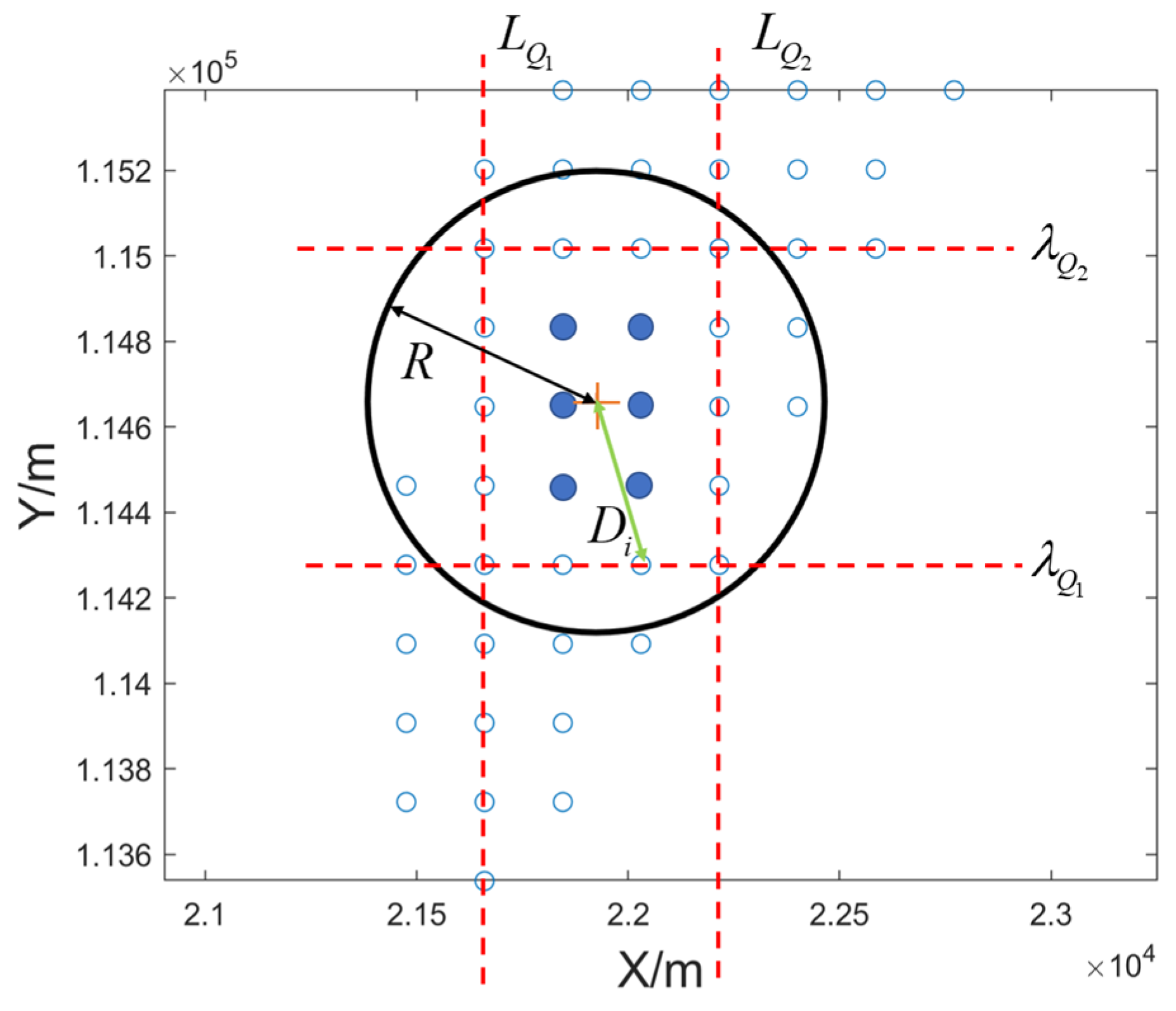
The point within the range circle and its weight relative to the overall point weight share are given by Equation (20).

3. Confidence Testing

To verify the generalization ability of the method, six groups of different gravity feature backgrounds were selected for the experiment, with a duration of 90 min for each voyage. The confidence level was also verified, the confidence intervals were calculated, and the robustness of the method was tested through 1000 iterations of sampling with hypothesis testing to prove the statistical significance of the results.

3.1. Relevance Calculation

The confidence level of the matching algorithm reacts to the reliability of the matching position, the larger the confidence level, the higher the reliability of the matching result, and the smaller the confidence level, the lower the reliability of the matching result. Therefore, there is a negative correlation with the matching position error. The validity of the proposed confidence method is verified by calculating the correlation between the confidence level and the matching error. The Spearman rank correlation coefficient was used to indicate the degree of correlation between the two sets of discrete data.

$$\begin{array}{l}P=(P_1, P_2,\dots ,P_n)\\ d=(d_1, d_2,\dots ,d_n)\end{array}$$

(21)

$$t_i=P_i^{\prime }-d_i^{\prime } \left(i=1,2,\dots n\right)$$

(22)

$${\rho }_s=1-{\displaystyle \frac{6{\displaystyle \sum t_i^2}}{t(t^2-1)}}$$

(23)

where $P$ is the confidence sequence, $d$ is the matching error size sequence, and $t$ denotes the length of the two columns of data. Ranking the values of $P$ and $d$. yields a ranking, $p_i^{\prime }$, corresponding to each $p_i$, and a ranking, $d_i^{\prime }$, corresponding to each $d_i$. Equation (22) calculates the difference between the ranking positions, and, finally, the degree of correlation between the two sets of data is obtained according to Equation (23). The correlation coefficient takes the range of [−1, 1], a correlation coefficient, $\rho$, of 1 means that the two columns of data are perfectly positively correlated, and a correlation coefficient of −1 means that they are perfectly negatively correlated.

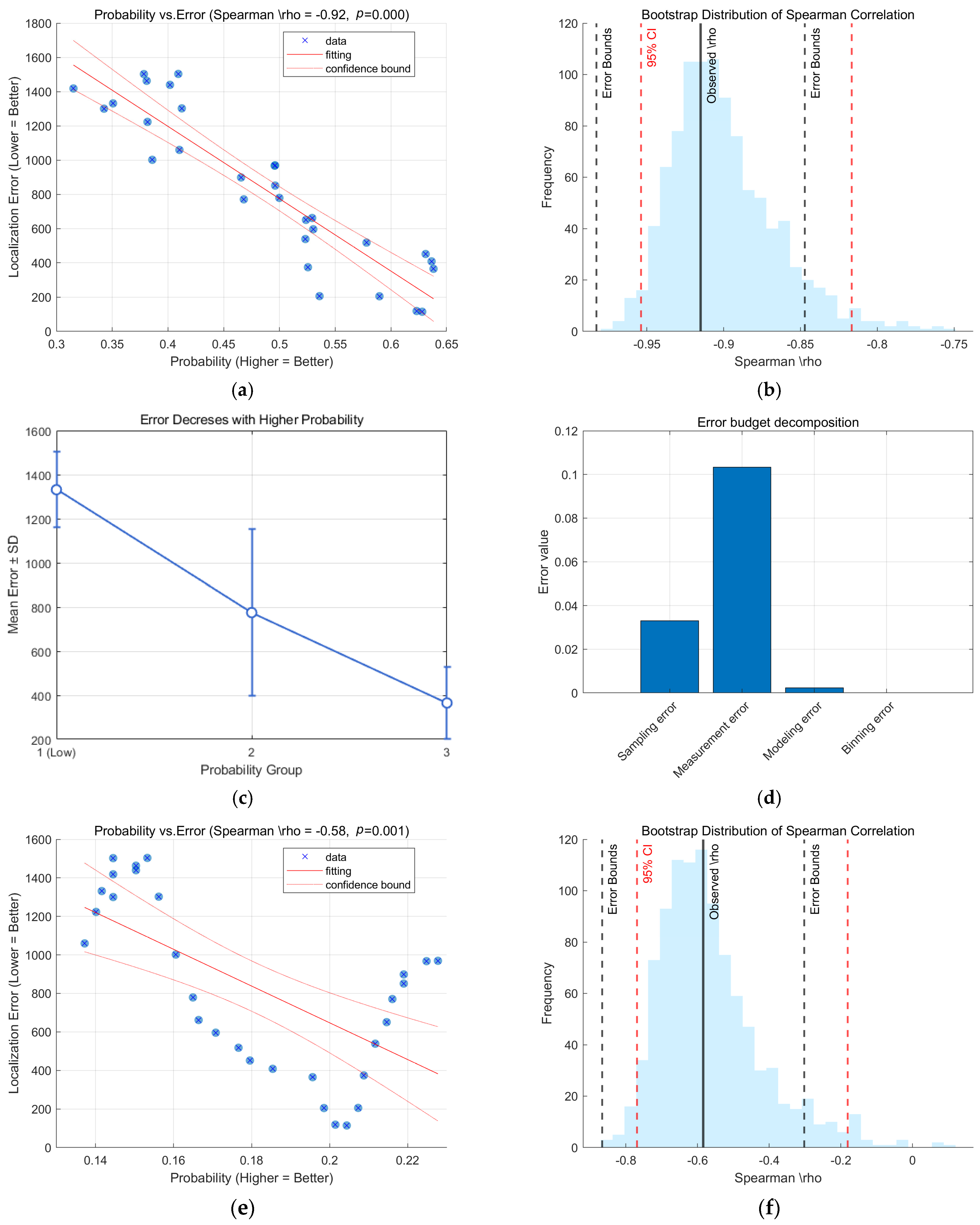
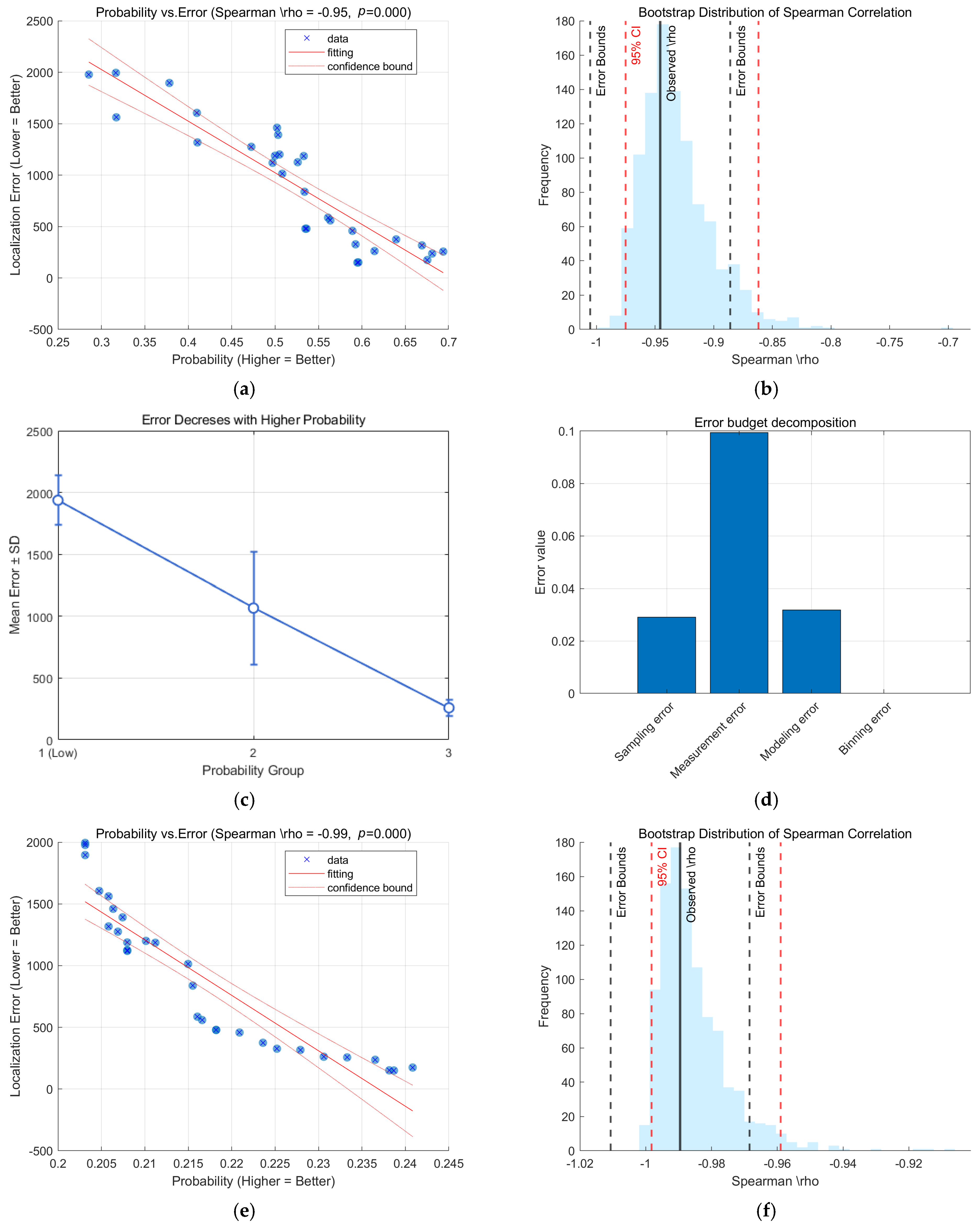
3.2. Hypothesis Testing

Original hypothesis: $H_0:{\rho }_s=0$ (no monotonic correlation).

Alternative assumptions: $H_1:{\rho }_s<0$ (negative correlation).

Test statistic:

$$Z={\rho }_s\sqrt{{\displaystyle \frac{n-2}{1-{\rho }_s^2}}}\sim t\left(n-2\right)$$

(24)

Bootstrap confidence intervals are used to verify the robustness of the correlation coefficients. The steps are as follows:

(1)

Resampling: $n$ samples are taken from the original data with putbacks and repeated $B=1000$ times to obtain $\left\{{\rho }_s^{\left(1\right)},{\rho }_s^{\left(2\right)},\dots ,{\rho }_s^{\left(B\right)}\right\}$;

(2)

Calculate the 95% confidence intervals: $CI=\left[{\rho }_s^{\left(B\times 0.025\right)},{\rho }_s^{\left(B\times 0.975\right)}\right]$;

(3)

If $CI$ does not contain 0, reject $H_0$.

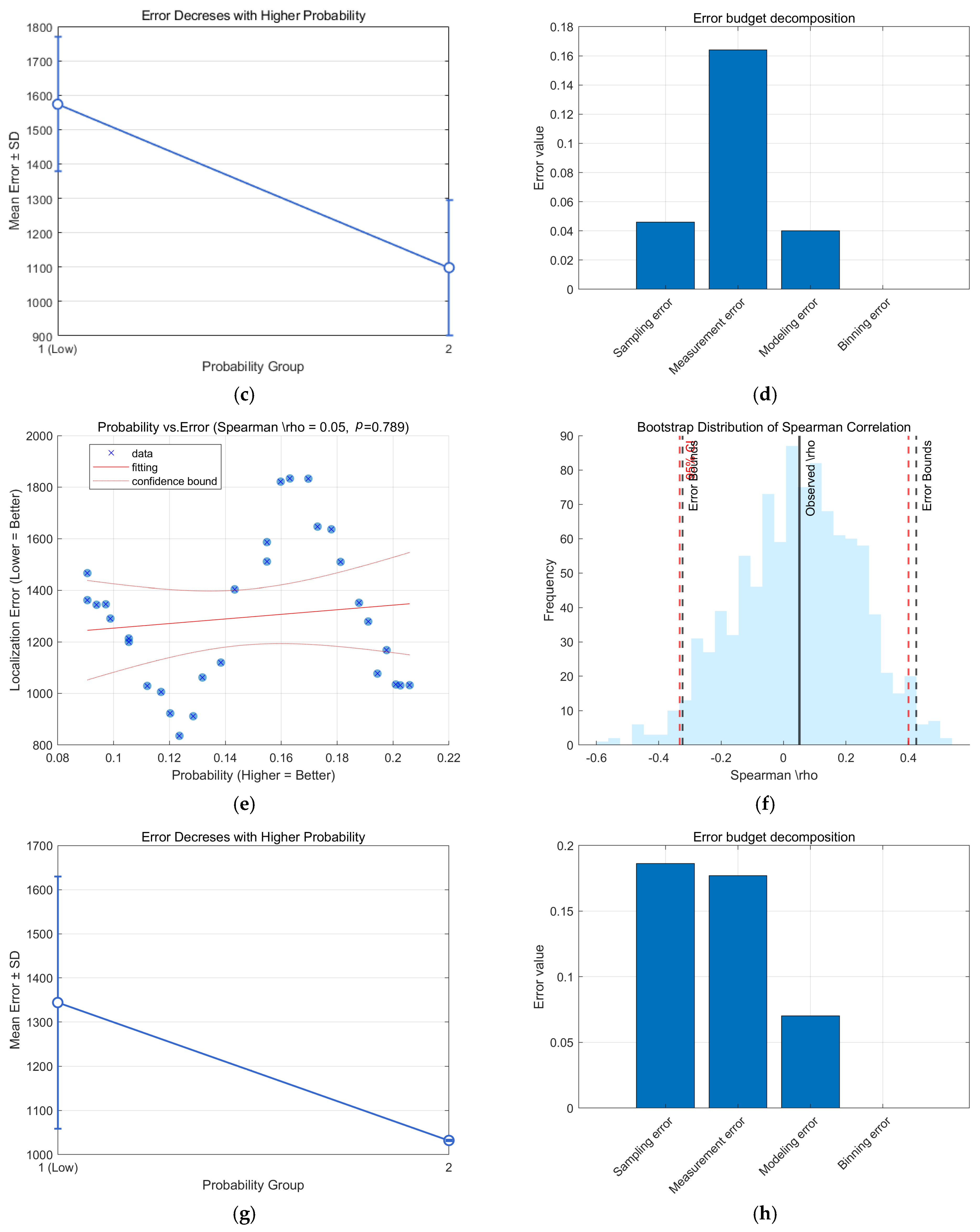
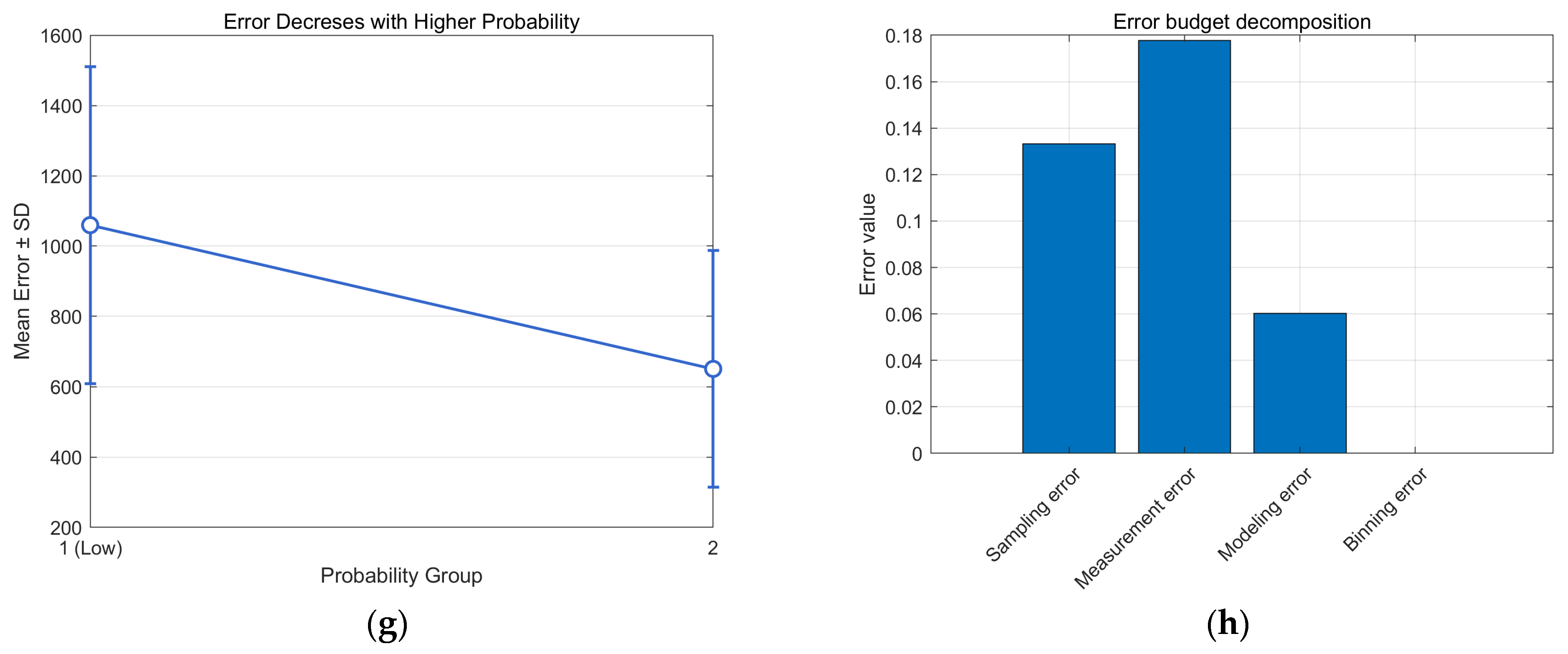
3.3. Trend Analysis of Split-Box

Boxed trend analysis involves dividing the range of values of a continuous variable into several intervals and then counting the number of data points in each interval for the statistical analysis.

Grouping method: $P$ was discretized into 5 groups by quartiles (0–20%, 20–40%, …, 80–100%).

The within-group error statistic with the mean is determined as per Equation (25) and the standard deviation as per Equation (26). Also, the median of each group was counted as an error characteristic.

$${\overline{d}}_k={\displaystyle \frac{1}{n_k}}{\displaystyle \sum _{i\in k}{d}_i}\left(k=1,2,\dots ,5\right)$$

(25)

$${\sigma }_k=\sqrt{{\displaystyle \frac{1}{n_k-1}}{{\displaystyle \sum _{i\in k}\left(d_i-{\overline{d}}_k\right)}}^2}$$

(26)

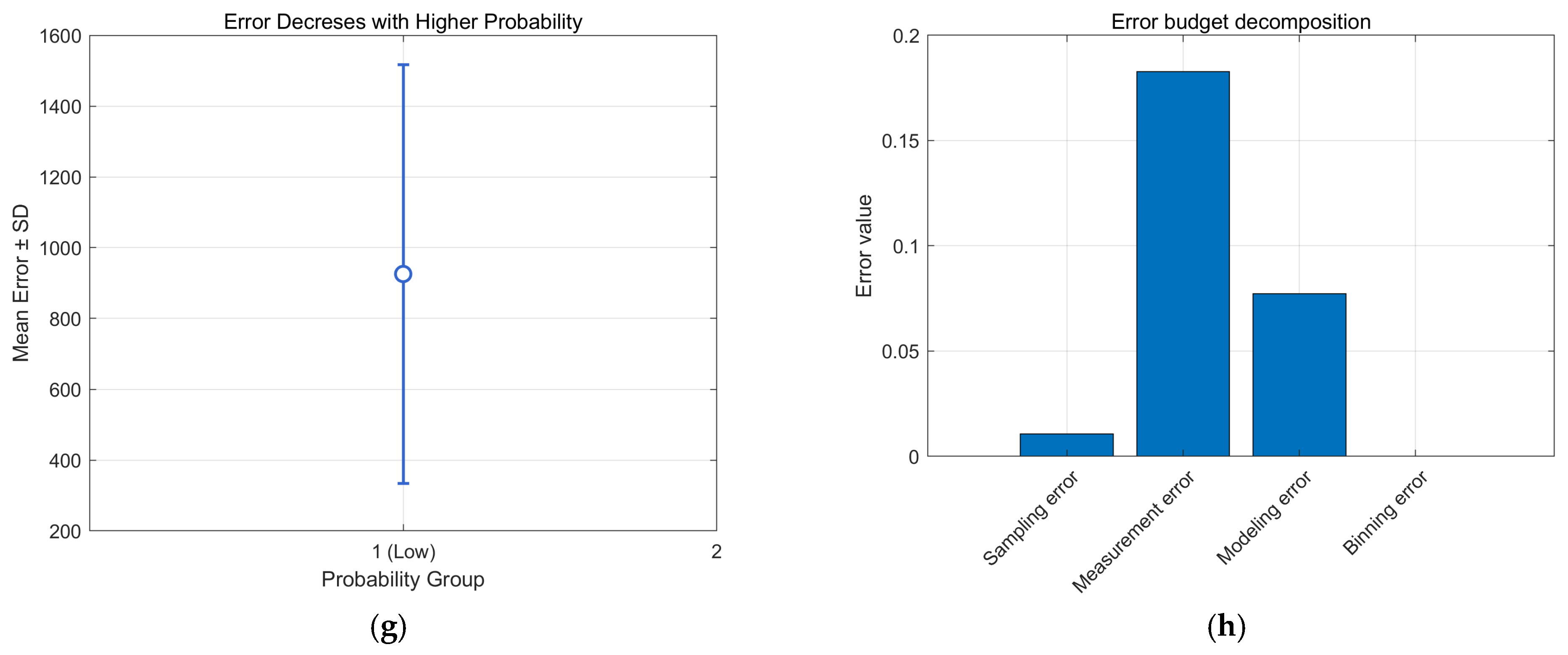
3.4. Error Bounds and Error Budget

Error bounds are used to quantify the range of uncertainty in the correlation estimates and are often used in conjunction with confidence intervals. The distribution of the correlation coefficients is calculated using the existing bootstrap sample (assuming it has been generated). The specific methodology is described below:

(1)

The median Spearman correlation coefficient is extracted from the bootstrap sample as a point estimate;

(2)

Its standard deviation is calculated as a benchmark for the error boundaries;

(3)

The error bound is defined as the point estimate ± k × SD, where k is chosen according to the confidence level (e.g., 95% corresponds to 1.96). SD is the standard deviation

The error budget is used to decompose the sources of total error and to specify the proportion of the contribution of different factors to the uncertainty of the results. In this paper, four errors are analyzed in terms of the sampling error, measurement error, modeling error, and binning error. The sampling error takes the bootstrap standard deviation. The measurement error, on the other hand, adds standard deviations to the confidence and matching errors, and the effect on the correlation is estimated by the covariance propagation formula. The modeling errors are analyzed by comparing the difference between the Spearman and Pearson correlation coefficients to assess the model fit. The binning errors were analyzed to determine the volatility of the results by comparing the changes in the different bins.

4. Experimental Results

The experimental data were from measured shipboard observations in the Pacific Ocean., in which a SAG-2M Jetlink gravimeter was used. The SAG-2M marine gravimeter is jointly developed by multiple Chinese institutions. With this data processing subsystem, filtered gravity anomalies can be output in real time and navigation information can be computed. At the same time, an onboard Global Navigation Satellite System (GNSS) provided the reference position. The DGM used in the experiment was from the Global Ocean Gravity Field $1\prime \times 1\prime$ model, produced by Sandwell which from Scripps Institution of Oceanography, University of California San Diego [29]. The performance parameters of the main sensors are shown in

Table 1. Main measuring equipment’s parameters.

Main Measuring Equipment Parameters
Parameter	Value
Gyro constant drift	$0.003°/\mathrm{h}$
Gyro random error	$0.0005°/\sqrt{\mathrm{h}}$
Accelerometer zero bias	10 µg
Accelerometer random drift	$3\mathrm{mGal}/\sqrt{\mathrm{hz}}$

. The data were all sampled at a frequency of $1\mathrm{Hz}$, and the resolution of the gravity anomaly map required for the match was $1^{\prime }\times 1^{\prime }$. Matching is carried out by extracting the inertial navigation position and measured gravity anomaly information at intervals of 180s, with every 10 intervals constituting a matching sequence. The matching process was carried out continuously by a sliding window, the search radius was $1^{\prime }$, and the sampling interval of the positions of the to-be-matched trajectories within the search range was $1^{\prime }/10$. With the final matching point as the center, and the precision error setting at $1^{\prime }/10\times 3$ as the radius of the drawing range circle, the first 49 trajectories of the similarity sequence were selected for analysis. The dataset consisted of ocean gravity anomaly maps, inertial navigation track coordinates, GNSS navigation track coordinates, and a sequence of gravity anomalies measured in real time by a gravimeter and then processed. The GNSS navigation track coordinates were used to validate the accuracy of the matching algorithm’s results.

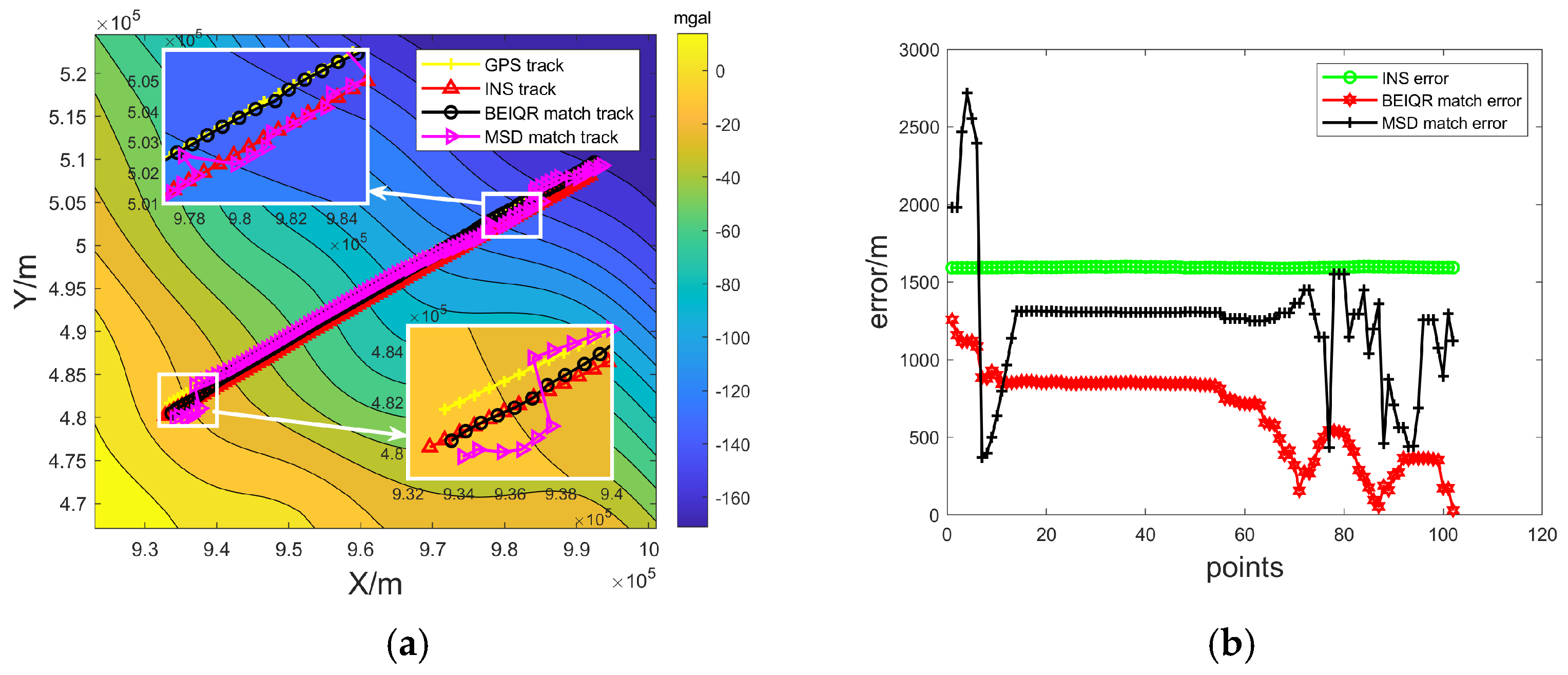
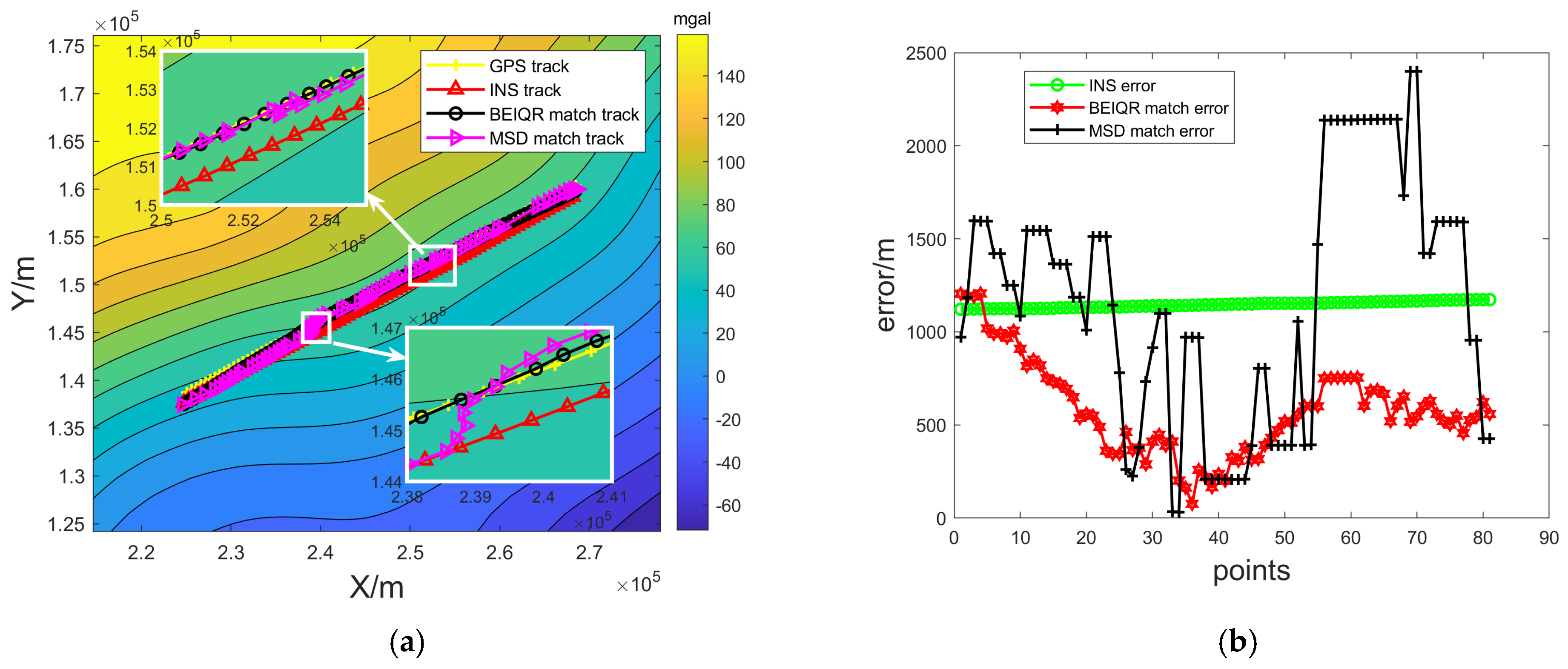
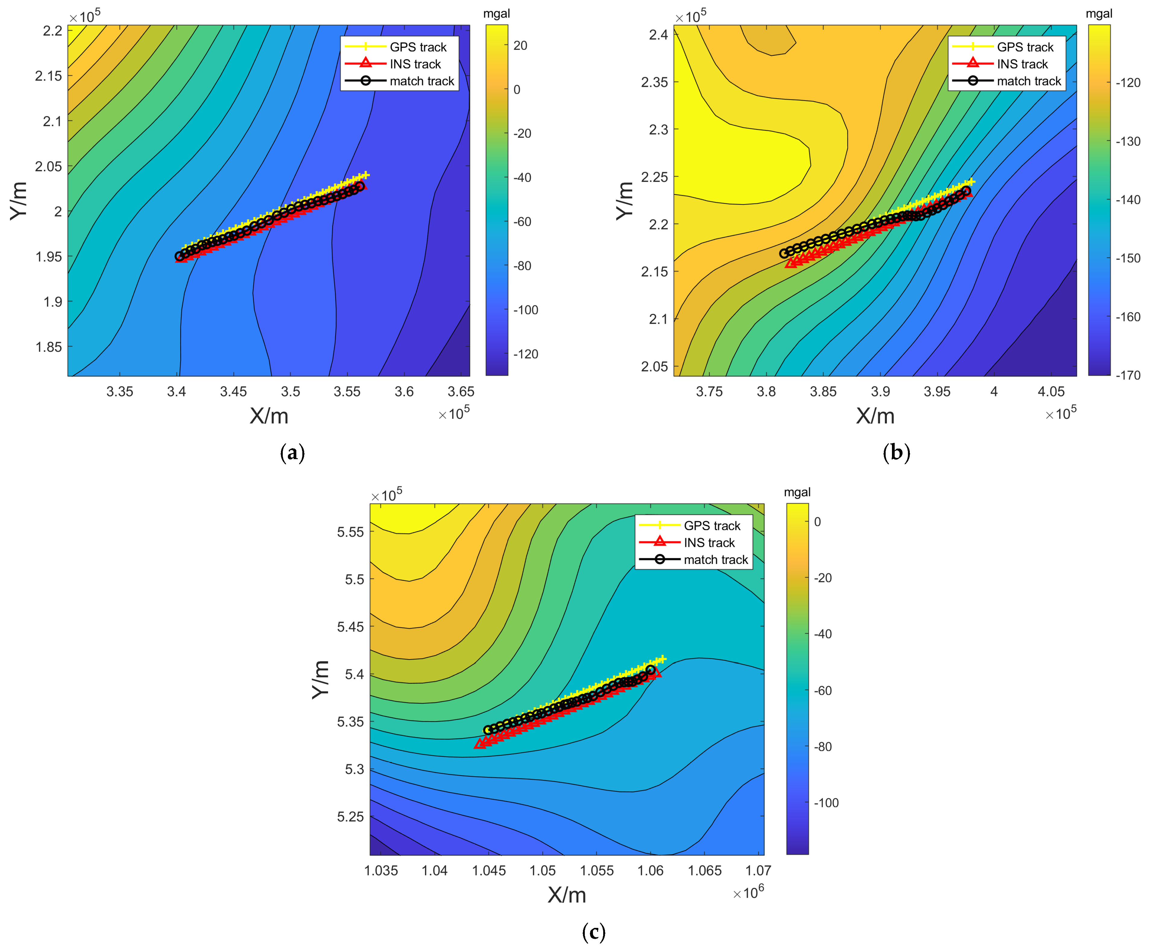
4.1. Experiments to Verify the Effectiveness of the Matching Algorithm

Two sets of trajectories in the different gravity field background headings were selected for experimental illustration. The first set of trajectory headings was selected to be perpendicular to the contour, as shown in Figure 3a, and the submersible was affected more by the noise of the gravimeter’s measurement in this case. The matching error is shown in Figure 3b. The second set of trajectory headings was selected parallel to the contour, as shown in Figure 4a, and the submersible was affected more by the zero-bias error of the gravimeter in this case. The matching error is shown in Figure 4b. The first set of experiments can avoid the defect of the single-point matching method being affected by the measurement noise, to a certain extent, by sequence matching, so the overall error of the MSD method is smaller than the inertial navigation. However, compared with the method proposed in this paper, the selection of the extreme point cannot avoid the interference of the zero bias of the measurement. The second group of experiments was greatly disturbed by the zero bias of the gravimeter, which led to the large fluctuation in the error of the MSD method, while the method proposed in this paper effectively avoided this situation, and the matching trajectory was stable, with a small and stable error.

From the two sets of matching results, it can be seen that the interquartile-range-matching method based on Bayesian estimation avoids the occurrence of large fluctuations in error. The reason for this is precisely that the algorithm does not use a single extreme point as the matching result but considers the positional distribution of multiple to-be-matched points, as well as the probabilistic weighting relationship of the to-be-matched points. Therefore, considering the final matching position, it has good stability.

4.2. Experiments to Verify the Validity of the Confidence Level

Confidence intervals, hypothesis testing, error bounds, and error budgets are also analyzed via the contents of Section 3 to verify the statistical significance of the results. Finally, the method in this paper is compared with the confidence method [21], which is also based on the TERCOM algorithm.

The different gravity field backgrounds selected for the six sets of experiments, along with the degree of correlation between the matching error and the confidence level, calculated using Equation (23), are listed in

Table 2. Experimental background and results.

Experiment	Variance	Information Entropy	Correlation Coefficient	Degree of Relevance		Confidence Interval
				BEIQRC	KTERCOMC	BEIQRC	KTERCOMC
1	1033.43	7.1843	−0.0076	−0.90	0.05	[−0.76, −0.95]	[0.32, 0.40]
2	358.68	7.6207	−0.1537	−0.92	−0.58	[−0.81, −0.95]	[−0.24, −0.75]
3	681.03	7.2725	0.2254	−0.95	−0.99	[−0.85, −0.97]	[−0.96, −0.99]
4	2562.93	7.5286	0.6596	−0.93	−0.97	[−0.83, −0.95]	[−0.88, −0.99]
5	13.03	7.3913	−0.4203	−0.92	−0.81	[−0.82, −0.96]	[−0.62, −0.92]
6	58.74	7.6711	−0.2576	−0.91	0.66	[−0.77, −0.97]	[0.26, 0.84]

. Due to space constraints, only the first three sets of experiments are visualized in this paper. To understand the experiments in different contexts, the characteristics of the trajectories of the first three sets of experiments and the environment of the gravity field in which they are located are given, as shown in Figure 5.

In experiment 1, a region with a large span of gravity field variation is selected, with a variance of 1033 mgal², information entropy of 7.1843, and correlation coefficient of −0.2276. The latitude and longitude correlation coefficients are low, as shown in Figure 5a. The horizontal coordinate is the confidence level, and the vertical coordinate is the matching error, which demonstrate the negative correlation between the matching error and its confidence level, as shown in Figure 6a, where the solid red line is the fitted curve, and the dashed line is the confidence interval of its fitted curve. As can be seen from Figure 6a, the first group of experiments selects points with confidence levels all less than 0.5, and as the confidence level increases, the matching error decreases accordingly, showing a significant negative correlation. The correlation between the two reaches −0.9, and its $p$ is 0, which is less than 0.05. This shows that the confidence level is significantly negatively correlated with the error. The bootstrap confidence intervals, obtained through hypothesis testing with 1000 resampling iterations with put-back, are shown in Figure 6b. To verify the robustness of the correlation coefficients, it reflects the reliability of the obtained correlation coefficients. The red dashed lines indicate confidence intervals, and the black dashed lines indicate error bounds with uncertainty ranges, where the lower limit of the error bounds exceeds −0.8. The error bounds are $-0.887\pm 0.090$. A trend analysis by the split-box method was conducted to validate the feasibility and robustness of the calculations and to reduce the complexity of the data, as shown in Figure 6c. The first set of experimental data is in split-box Group I and Group II, where the mean value within 20–40% of the domain of Group I is 1586.5m, the standard deviation is 194.98 m, and the median is 1573.68 m. The mean value within the second set of domains (40–60%) is 1149.9 m, the standard deviation is 197.02 m, and the median is 1098.33 m. It is demonstrated that as the confidence trend increased, the error trend decreased, which aligns with the original intention of the confidence design in this paper, as shown in Figure 6.

In this paper, we also conduct a confidence method comparison experiment based on the literature [22], which is referred to as KTERCOMC for ease of expression. The degree of correlation was calculated using Spearman, and Figure 6e shows that the experimental results do not present a correlation. The method requires a high distribution of the preorder matching error. However, the preorder matching error is not well and evenly distributed between the maximum and minimum of the error range, resulting in the inability to reflect the correlation between the two.

In experiment 2, the variance of the gravity field features is 358.68 mgal², the information entropy is 7.6207, and the correlation coefficient is −0.1537. The trajectory position corresponds to a smaller span of the gravity field, sailing at a 45° angle to the contour, as shown in Figure 5b. A trend relationship between the matching confidence and matching accuracy is similarly demonstrated, with a Spearman’s correlation of −0.92 and a p-value of 0, which is less than 0.05, as shown in Figure 7a. It shows that the confidence level is significantly negatively correlated with the error. The minimum value of the confidence interval was verified to be greater than 80% via 1000 hypothesis tests. The minimum value of the uncertainty range error bound is close to −0.85, as shown in Figure 7b. The error bounds is $-0.901\pm 0.065$. The split-box method demonstrates the mean and standard deviation of the corresponding errors over the three confidence level value domains, as shown in Figure 7c. The mean value of the error contained in 20–40% of the first domain is 1320.2 m, the standard deviation is 170.66 m, and the median is 1331.43 m. The mean value of the error contained in the second domain of 40–60% is 793.97 m, with a standard deviation of 376.79 m, and the median is 774.92 m. The mean value of the error contained in the third domain 60–80% is 291.59 m, with a standard deviation of 162.68 m, and the median is 365.04 m. The comparison from domain to domain significantly illustrates that the confidence level is a good reflection of the trend in the error.

In [21], comparison experiments similar to that shown in Figure 7e can be seen, where the confidence level is less than 0.2. The confidence feedback of the error is more obvious, showing a more significant negative correlation trend. However, the portion higher than 0.2 does not correctly illustrate the negative correlation law between the error and the confidence level.

In experiment 3, the variance in the gravity field’s features is 681.03 mgal², the information entropy is 7.2725, and the correlation coefficient is 0.2254. A section of the trajectory is selected to sail from a dense region of contours to a sparse region of contours, with the heading ranging from parallel to the contours to a 45° angle with the contours. The gravity field in the direction of the latitude and longitude exhibits a positive correlation, as shown in Figure 5c. The relationship between the matching results and the confidence level of the aforementioned method is depicted, showing a strong linear trend, with nearly all points falling within the confidence interval, as shown in Figure 8a. The error confidence levels for less than 550 m were all greater than 50% and reached −0.95 between the two, as determined by Spearman’s correlation, and had a $p$ of 0, which is less than 0.05. It shows that the confidence level is significantly negatively correlated with the error. The minimum value of the validation confidence interval exceeds −0.85, and the minimum value of the uncertainty error bound is close to −0.9 via 1000 hypothesis tests, as shown in Figure 8b. The error bounds are $-0.932\pm 0.057$. The split-box method demonstrates the mean and standard deviation of the corresponding error over the three confidence-level value domains, as shown in Figure 8c. The mean value of the error contained in the first domain of 20–40% is 1857.5 m, the standard deviation is 201.87 m, and the median is 1936.85 m. The mean value of the error contained in the second domain of 40–60% is 895.43 m, the standard deviation is 456.23 m, and the median is 1066.38 m. The mean value of the error contained in the third domain 60–80% is 270.15 m, the standard deviation is 68.862 m, and the median is 258.98 m.

Compared with the literature [21], in the experiment, as shown in Figure 8e, the method achieved a more significant confidence law feature in experiment 3, and Spearman’s correlation coefficient showed a correlation between the error and the confidence level as high as −0.99. The lower limit of the confidence interval in Figure 8f reaches −0.96, which significantly reflects the strong negative correlation between the confidence and error. However, observation of the confidence values reveals that the large span of errors corresponds to a very small span of confidence levels, all of which are concentrated between 0.2 and 0.25. Although it shows a changing trend, the confidence level with less than a 500 m matching error is less than 0.3. The relationship between the error and confidence cannot be effectively reflected in a confidence range of 0 to 1.

A gravity field with a large latitude and longitude correlation coefficient and a variance of 2562.93 mgal² was selected for experiment 4. The trajectory travels in a region where the gravity field spans a large area; the contours change in a gradient with the latitude and longitude; and the heading is in the same direction as the gradient descent, but it is disturbed by noise, which tends to produce a matching deviation parallel to the heading. The correlation coefficient between the matching error and confidence level is as high as −0.95, reflecting the fact that the method proposed in this paper is able to represent the error variations well through the confidence level. A region with a gravity field variance of only 13.03 mgal² was selected for experimental validation in experiment 5, with gravity anomalies spanning from 4 to 18 mgal². The submarine navigates in a region where the fluctuations of the gravity field vary particularly gently, and the gravity measurement noise tends to produce large disturbances, such that there is no effective directionality between consecutive matching points and it is impossible to judge using conventional confidence methods. The method proposed in this paper verifies that the correlation coefficient between the matching error and confidence level is as high as −0.92, which is also able to reflect the error changes effectively. Experiment 6 selects a region with a small gravity field variance of only 58.74 mgal², a gravity anomaly spanning from −30 to −10 mgal², and an information entropy of 7.6711 for the experiment. The submarine heading is parallel to the gravity anomaly contour, which is interfered with by the zero bias of the gravimeter, leading to a match bias parallel to the contour. The correlation coefficient between the matching error and the confidence level is as high as −0.91.

As shown in

Table 3. Error budget decomposition.

		Sampling Error	Measurement Error	Modeling Error	Binning Error	Total Error
	1	0.04596	0.16408	0.04008	0	0.17505
BEIQRC	2	0.03300	0.10337	0.00234	0	0.10854
	3	0.02902	0.09939	0.03177	0	0.10831
	1	0.18619	0.17713	0.07029	0	0.26643
KTERCOMC	2	0.13328	0.17763	0.06016	0	0.23008
	3	0.01066	0.18277	0.07719	0	0.19869

, in both the BEIQRC and KTERCOMC methods, the results of the three strategies of binning for the three sets of experiments are consistent for all three strategies, so there is no binning error. Comparing the sampling errors, it can be seen that the BEIQRC method’s error is significantly better than the KTERCOMC method’s for the first two sets of experiments. For the third set of experiments, the correlation coefficient of the KTERCOMC method is extremely high, and, therefore, its sampling error is small. The stability of the BEIQRC method is better than that of the KTERCOMC method in terms of both the measurement error and modeling error.

The confidence method proposed in this paper circumvents the risk introduced by previous scholars using pre-matching results to analyze the accuracy of current matching results. Avoiding erroneous confidence judgments on subsequent matches due to preorder mismatching is an independent evaluation method based on the characteristics of the algorithm itself.

5. Conclusions

By calculating the Bayesian posterior probability of the to-be-matched points, the prior coordinate distribution of the similarity sequence is investigated, and the interquartile range method is used to perform position correction for gravity-aided inertial navigation. Using these coordinates as the center of the circle and the accuracy requirement as the radius, the to-be-matched points within its range are calculated. The distance of the to-be-matched points is analyzed along with the weight of the measurement to obtain the confidence level of the matching results. The results of multiple sets of experiments in Section 2 and Section 4 show that the interquartile range localization algorithm based on Bayesian estimation proposed in this paper, as well as its underwater localization confidence method research, are effective. The reliability analysis of the matching results is better realized under the preliminaries of improving the matching accuracy. The degree of confidence reliability is verified by a confidence test. The algorithm in this paper provides an effective reference for gravity-aided inertial navigation positioning accuracy. In future work, we will consider more factors that interfere with the matching process, such as accelerometer fixation errors, as well as analyze the gravimeter measurement noise and gravity field noise separately in order to conduct a more informative study.

References

1. Liu, B.; Wei, S.; Lu, J.; Wang, J.; Su, G. Fast Self-Alignment Technology for Hybrid Inertial Navigation Systems Based on a New Two-Position Analytic Method. IEEE Trans. Ind. Electron. 2020, 67, 3226–3235. [Google Scholar] [CrossRef]
2. Zhao, S.; Zheng, W.; Li, Z.; Xu, A.; Zhu, H. Improving Matching Accuracy of Underwater Gravity Matching Navigation Based on Iterative Optimal Annulus Point Method with a Novel Grid Topology. Remote Sens. 2021, 13, 4616. [Google Scholar] [CrossRef]
3. Jia, Y.; Li, S.; Qin, Y.; Cheng, R. Error Analysis and Compensation of MEMS Rotation Modulation Inertial Navigation System. IEEE Sens. J. 2018, 18, 2023–2030. [Google Scholar] [CrossRef]
4. Ma, T.; Ding, S.; Li, Y.; Fan, J. A Review of Terrain Aided Navigation for Underwater Vehicles. Ocean Eng. 2023, 281, 114779. [Google Scholar] [CrossRef]
5. Xiong, C.; Wu, L.; Liu, S.; Mao, G.; Wu, P.; Ji, B.; Bao, L.; Wang, Y. A Novel Eötvös Correction Method Based on Passive Velocity Compensated INS. IEEE Trans. Instrum. Meas. 2025, 74, 1–12. [Google Scholar] [CrossRef]
6. Wang, S.; Zheng, W.; Li, Z. Optimizing Matching Area for Underwater Gravity-Aided Inertial Navigation Based on the Convolution Slop Parameter-Support Vector Machine Combined Method. Remote Sens. 2021, 13, 3940. [Google Scholar] [CrossRef]
7. Zhao, S.; Xiao, X.; Pang, X.; Wang, Y.; Deng, Z. Gravity Matching Algorithm Based on Backtracking for Small Range Adaptation Area. IEEE Trans. Instrum. Meas. 2024, 73, 1–13. [Google Scholar] [CrossRef]
8. Wang, Z.; Huang, Y.; Wang, M.; Wu, J.; Zhang, Y. A Computationally Efficient Outlier-Robust Cubature Kalman Filter for Underwater Gravity Matching Navigation. IEEE Trans. Instrum. Meas. 2022, 71, 1–18. [Google Scholar] [CrossRef]
9. Zou, J.; Cai, T. Improved Particle Swarm Optimization Screening Iterative Algorithm in Gravity Matching Navigation. IEEE Sens. J. 2022, 22, 20866–20876. [Google Scholar] [CrossRef]
10. Mao, N.; Li, A.; Xu, J.; Li, F.; Qin, F.; He, H.; Li, J.; Zhu, B. Adaptive Gravity-Aided Inertial Navigation Based on Characteristic Analysis of Marine Gravity Anomaly From Satellite Altimetry. IEEE Trans. Geosci. Remote Sens. 2024, 62, 1–13. [Google Scholar] [CrossRef]
11. Zhao, S.; Xiao, X.; Deng, Z.; Shi, L. Gravity Matching Algorithm Based on Correlation Filter. IEEE Sens. J. 2023, 23, 2618–2629. [Google Scholar] [CrossRef]
12. Zhao, X.; Zheng, W.; Xu, K.; Zhang, H. Optimizing the Matching Area for Underwater Gravity Matching Navigation Based on a New Gravity Field Feature Parameters Selection Method. Remote Sens. 2024, 16, 2202. [Google Scholar] [CrossRef]
13. Wang, B.; Zhu, Y.; Deng, Z.; Fu, M. The Gravity Matching Area Selection Criteria for Underwater Gravity-Aided Navigation Application Based on the Comprehensive Characteristic Parameter. IEEE/ASME Trans. Mechatron. 2016, 21, 2935–2943. [Google Scholar] [CrossRef]
14. Wang, B.; Li, T.; Deng, Z.; Fu, M. Wavelet Transform Based Morphological Matching Area Selection for Underwater Gravity Gradient-Aided Navigation. IEEE Trans. Veh. Technol. 2023, 72, 3015–3024. [Google Scholar] [CrossRef]
15. Wang, C.; Wang, B.; Deng, Z.; Fu, M. A Delaunay Triangulation-Based Matching Area Selection Algorithm for Underwater Gravity-Aided Inertial Navigation. IEEE/ASME Trans. Mechatron. 2021, 26, 908–917. [Google Scholar] [CrossRef]
16. Wang, S.; Cheng, G.; Zhao, J. The Study on the TERCOM Mismatch Diagnostic Based on Detecting the Extreme Value of Similarity. In Proceedings of the 2011 Second International Conference on Mechanic Automation and Control Engineering, Inner Mongolia, China, 15–17 July 2011; pp. 4623–4626. [Google Scholar]
17. Zhao, S.; Zheng, W.; Li, Z.; Zhu, H.; Xu, A. Improving Matching Efficiency and Out-of-Domain Positioning Reliability of Underwater Gravity Matching Navigation Based on a Novel Domain-Center Adaptive-Transfer Matching Method. IEEE Trans. Instrum. Meas. 2023, 72, 1–11. [Google Scholar] [CrossRef]
18. Zhao, S.; Zheng, W.; Li, Z.; Zhu, H.; Xu, A. Improving Matching Efficiency and Out-of-Domain Reliability of Underwater Gravity Matching Navigation Based on a Novel Soft-Margin Local Semicircular-Domain Re-Searching Model. Remote Sens. 2022, 14, 2129. [Google Scholar] [CrossRef]
19. Han, Y.; Wang, B.; Deng, Z.; Wang, S.; Fu, M. A Mismatch Diagnostic Method for TERCOM-Based Underwater Gravity-Aided Navigation. IEEE Sens. J. 2017, 17, 2880–2888. [Google Scholar] [CrossRef]
20. Zhao, S.; Zheng, W.; Li, Z.; Zhu, H.; Xu, A. A Novel Cross-Line Adaptive Domain Matching Algorithm for Underwater Gravity Aided Navigation. IEEE Geosci. Remote Sens. Lett. 2024, 21, 1–5. [Google Scholar] [CrossRef]
21. Gao, S.; Cai, T. A Confidence Assessment Method for Positioning Errors in Gravity-Aided Navigation. In Proceedings of the 2023 International Conference on Ocean Studies (ICOS), Vladivostok, Russia, 3–6 October 2023; pp. 007–010. [Google Scholar]
22. Han, Y.; Wang, B.; Deng, Z.; Fu, M. An Improved TERCOM-Based Algorithm for Gravity-Aided Navigation. IEEE Sens. J. 2016, 16, 2537–2544. [Google Scholar] [CrossRef]
23. Ma, Z.; Wang, B.; Bi, R. A Mismatch Correction Method Based on Two-Way Strategies of Spatial Vector Feature. In Proceedings of the 2024 IEEE 18th International Conference on Control & Automation (ICCA), Reykjavík, Iceland, 18–21 June 2024; pp. 573–578. [Google Scholar]
24. Yang, Y.; Wang, K. Mismatching Judgment Using PDAF in ICCP Algorithm. In Proceedings of the 2008 Fourth International Conference on Natural Computation, Jinan, China, 18–20 October 2008; Volume 4, pp. 172–176. [Google Scholar]
25. Li, Z.; Zheng, W.; Wu, F. Improving the Reliability of Underwater Gravity Matching Navigation Based on a Priori Recursive Iterative Least Squares Mismatching Correction Method. IEEE Access 2020, 8, 8648–8657. [Google Scholar] [CrossRef]
26. Yoo, Y.M.; Lee, W.H.; Lee, S.M.; Park, C.G.; Kwon, J.H. Improvement of TERCOM Aided Inertial Navigation System by Velocity Correction. In Proceedings of the 2012 IEEE/ION Position, Location and Navigation Symposium, Myrtle Beach, SC, USA, 23–26 April 2012; pp. 1082–1087. [Google Scholar]
27. Wang, B.; Cai, T.; Fang, K. Observation-Differenced Point Mass Filter in Gravity-Aided Inertial Navigation. IEEE/ASME Trans. Mechatron. 2024, 29, 1601–1606. [Google Scholar] [CrossRef]
28. Yurong, H.; Bo, W.; Zhihong, D.; Mengyin, F. Point Mass Filter Based Matching Algorithm in Gravity Aided Underwater Navigation. J. Syst. Eng. Electron. 2018, 29, 152–159. [Google Scholar] [CrossRef]
29. Sandwell, D.T.; Mueller, R.D.; Smith, W.H.F.; Garcia, E.; Francis, R. New Global Marine Gravity Model from CryoSat-2 and Jason-1 Reveals Buried Tectonic Structure. Science 2014, 346, 65–67. [Google Scholar] [CrossRef]
Figure 1. Schematic diagram of the single matching.
Remotesensing 17 02137 g001
Figure 2. Flow chart.
Remotesensing 17 02137 g002
Figure 3. Analysis of the results of the first group of BEIQR matches: (a) matching trajectories; (b) error diagram.
Remotesensing 17 02137 g003
Figure 4. Analysis of the results of the second group of BEIQR matches: (a) matching trajectories; (b) error diagram.
Remotesensing 17 02137 g004
Figure 5. Gravity field of the trajectory: (a) experiment 1’s matching trajectories and gravity fields; (b) experiment 2’s matching trajectories and gravity fields; (c) experiment 3’s matching trajectories and gravity fields.
Remotesensing 17 02137 g005
Figure 6. Illustration of experiment 1: (a) BEIQRC confidence and error relationships; (b) BEIQRC hypothesis test confidence intervals; (c) BEIQRC split-box trend analysis; (d) BEIQRC error budget decomposition; (e) KTERCOMC confidence and error relationships; (f) KTERCOMC hypothesis test confidence intervals; (g) KTERCOMC split-box trend analysis; (h) KTERCOMC error budget decomposition.
Remotesensing 17 02137 g006aRemotesensing 17 02137 g006b
Figure 7. Illustration of experiment 2: (a) BEIQRC confidence and error relationships; (b) BEIQRC hypothesis test confidence intervals; (c) BEIQRC split-box trend analysis; (d) BEIQRC error budget decomposition; (e) KTERCOMC confidence and error relationships; (f) KTERCOMC hypothesis test confidence intervals; (g) KTERCOMC split-box trend analysis; (h) KTERCOMC error budget decomposition.
Remotesensing 17 02137 g007aRemotesensing 17 02137 g007b
Figure 8. Illustration of experiment 3: (a) BEIQRC confidence and error relationships; (b) BEIQRC hypothesis test confidence intervals; (c) BEIQRC split-box trend analysis; (d) BEIQRC error budget decomposition; (e) KTERCOMC confidence and error relationships; (f) KTERCOMC hypothesis test confidence intervals; (g) KTERCOMC split-box trend analysis; (h) KTERCOMC error budget decomposition.
Remotesensing 17 02137 g008aRemotesensing 17 02137 g008b