Abstract
A linear frequency modulation (LFM) signal and its corresponding de-chirp operation are one of the basic methods for wideband radar signal processing, which can reduce the burden of the radar system sampling rate and is more suitable for large-bandwidth signal processing. More importantly, most existing methods against interrupted sampling repeater jamming (ISRJ) are based on time–frequency (TF) or frequency domain analysis of the de-chirped signal. However, the above anti-ISRJ methods cannot be directly applied to multiple-input multiple-output (MIMO) radar with multiple beams, because the angular waveform (AW) in mainlobe directions does not possess the TF properties of the LFM signal. Consequently, this work focuses on the co-optimization of transmit beampattern and AW similarity in wideband MIMO radar systems. Different from the existing works, which only concern the space–frequency pattern of the transmit waveform, we recast the transmit beampattern and AW expressions for wideband MIMO radar in a more compact form. Based on the compact expressions, a co-optimization model of the transmit beampattern and AWs is formulated where the similarity constraint is added to force the AW to share the TF properties of the LFM signal. An algorithm based on the alternating direction method of multipliers (ADMM) framework is proposed to address the aforementioned problem. Numerical simulations show that the optimized waveform can form the desired transmit beampattern and its AWs have similar TF properties and de-chirp results to the LFM signal.
1. Introduction
Compared with conventional radar, the main advantage of multiple-input multiple-output (MIMO) radar is its capacity for waveform diversity at the transmitter, which provides enhanced performance of parameter estimation, the transmit beampattern, and target detection [1,2,3]. Therefore, waveform design is an important topic for MIMO radar systems. In this paper, we focus on the waveform design for the desired transmit beampattern and angular waveform (AW) synthesis.
For narrowband MIMO radar, there are extensive works on the design of the transmit beampattern [4,5,6,7,8,9,10,11,12,13]. According to the waveform generation steps, these methods can be divided into two categories. The first category is the two-step method [4,5,6]. Because the transmit beampattern is determined by the waveform correlation matrix, this type of method first obtains the optimal correlation matrix and then generates constant-modulus (CM) waveforms according to the optimal correlation matrix. The second category is the one-step method, which directly generates CM waveforms by advanced non-convex optimization algorithms [7,8,9,10,11,12,13]. For wideband MIMO radar, there is little research focused on the transmit beampattern design, and most works focus on the spatial-frequency pattern of the transmit waveform [14,15,16,17]. Based on an exhaustive review of the existing literature, it seems that only the work in [18] considered the transmit beampattern design in wideband MIMO radar, where the beampattern matching error and the AW power spectral density (PSD) matching error were jointly minimized. Other work [14,15,16,17] mainly considered CM waveform optimization for spatial-frequency pattern matching or space–frequency nulling, using techniques such as the alternating direction method of multipliers (ADMM), alternating iteration, and majorization–minimization to obtain CM waveforms.
According to the beampattern shape, transmit beampatterns can be divided into wide-beam beampatterns or multi-beam beampatterns. A wide-beam beampattern has a large radiation space, which is more suitable for the search stage and scene information acquisition [19,20]. A multi-beam beampattern has multiple mainlobes with high transmit gain, which is more suitable for multiple target tracking or imaging and can improve the date rate and dwell time [18,21,22]. For the multi-beam beampattern situation, the target directions are known. Therefore, a corresponding signal processing strategy was proposed in [23,24], where receive beamforming is first performed, and then the pulse compression operation for AWs is performed. Consequently, the characteristics of AWs, rather than the waveform from each transmit element, are directly related to the target detection performance of radar. For narrowband MIMO radar, most works considered the quasi-orthogonality design of AWs to obtain a low range sidelobe level and avoid mutual interference between different AWs [8,9,10]. In [24], the PSD shape of AWs and the ambiguity function of AWs were also considered for narrowband MIMO radar. To the best of our knowledge, for wideband MIMO radar, only the work in [18] considered the design of AWs, where the PSD matching error of AWs was minimized in the objective function.
A transmit waveform with a large time–bandwidth product can enable the radar to achieve high range resolution, which has important applications in high-precision ranging and imaging fields [25,26]. The linear frequency modulation (LFM) signal is one of the most frequently used large time–bandwidth product signals in modern high-resolution radar systems, which also benefits from the de-chirp operation of the LFM signal, which can reduce the computation burden of pulse compression. Recently, a novel mainlobe jamming strategy named interrupted sampling repeater jamming (ISRJ) was proposed, which can not only raise the sidelobe level but also form false targets to mislead the radar [27]. In [28,29,30,31,32,33], based on the time–frequency (TF) analysis of a de-chirped signal, the anti-ISRJ strategy was proposed, and a frequency filter or TF filter was constructed to extract the real target echo. For the multiple target tracking situation, the ISRJ can serve as a self-defensive jammer to protect targets. However, because the TF properties of AWs are inconsistent with those of LFM, the above anti-ISRJ can not be directly applied to multi-beam scenarios.
Motivated by the problems in existing wideband MIMO radar waveform design, this work proposes a co-optimization framework for transmit beampattern and AW similarity in wideband MIMO radar systems. The main contributions of this paper can be summarized as follows:
- Different from the existing works where only the space–frequency pattern is considered, in this paper, the transmit beampattern and AW expressions for wideband MIMO radar are recast as a more compact form.
- Based on the compact forms of the transmit beampattern and AW, we extend the design concept of the transmit beampattern and the similarity analysis of the AW in narrowband MIMO radar to the wideband MIMO radar model. Then, a transmit beampattern design problem under AM similarity and CM constraints is formulated.
- An algorithm based on the ADMM framework is proposed to address the aforementioned problem. Some improvements are proposed to reduce the computational complexity, and the final computational complexity analysis is given. Numerical simulations show that the optimized waveform can form the multi-beam beampattern and its AWs can realize the de-chirp operation.
The rest of this paper is organized as follows. Section 2 introduces the signal model of wideband MIMO radar. In Section 3, the cost function of the joint design of transmit beampattern and AW similarity is proposed. In Section 4, the algorithm for the proposed joint optimization model is introduced and the computational complexity is given. Several simulation results are shown in Section 5. In Section 6, some discussions are given to further clarify the performance of the proposed method. Conclusions are drawn in Section 7.
Notation: Standard-case letters stand for scalars. Bold uppercase letters and bold lowercase letters denote matrices and vectors, respectively. The notations , , and denote the transpose, the conjugate, and the conjugate transpose, respectively. denotes the vectorization matrix operation. represents a diagonal matrix with its main diagonal filled with . ⊗ denotes the Kronecker product and ⊙ denotes the Hadamard product. The subscript denotes the Euclidean vector norm. is the imaginary part of the complex variable and is the real part of the complex variable. denotes the modulus operation. For a vector, the operations , , and are imposed in an elementwise way. denotes an identity matrix and denotes an vector of ones. j denotes the imaginary unit.
2. Signal Model
Consider a colocated wideband MIMO radar system with M transmit elements. The signal transmitted by the m-th element can be written as
where is the baseband signal, is the carrier frequency, and is the pulse duration.
It is assumed that the bandwidth of baseband signal is , and it is discretized by the sampling period . Then, the baseband signal can be expressed as , where denotes the code length. Let be the l-th sample of the M transmit waveforms, and the transmit waveform matrix can be written as . The discrete frequency spectrums of the transmit waveform matrix can be written as
where and the discrete Fourier transform (DFT) matrix can be expressed as . It is known that .
Considering a uniform linear array (ULA) with element spacing d, the transmit steering vector at frequency can be written as
and the frequency spectrums of the AW at the angle can be represented as
Let
and (4) can be rewritten in a more compact form as follows:
where . Then, the transmit beampattern of wideband MIMO radar can be defined as
where .
3. Problem Formulation
In this section, a co-optimization model of the transmit beampattern and AWs is formulated.
3.1. Multi-Beam Beampattern Design
In this subsection, the idea of conservation of energy is utilized to design a transmit beampattern with multiple beams. Following this idea, the beampattern optimization can be reduced to a three-point matching problem to satisfy the transmit gain and beamwidth requirements. It is supposed that there are N beams pointing at , respectively. For a ULA with element spacing , where denotes the speed of light, the Rayleigh beamwidth (distance from peak to first null) is about . Therefore, to control the beamwidth, it is desired that
Next, we will find a proper desired transmit gain value to guarantee the transmit gain. It is assumed that and the total transmit power can be calculated by
Under the assumption of allocating 100% transmitted power to the mainlobe angular sectors, we have
where denotes the power proportion of the n-th mainlobe. Let denote the LFM signal, and we construct the following transmit waveform matrix:
where . It can be seen that the above transmit waveform matrix can achieve the maximum transmit power gain at angle , and its beam has the most intense directivity compared with that of other waveforms. Therefore, the desired transmit gain value can be obtained by the transmit waveform in (13). Let denote the transmit beampattern of the transmit waveform in (13), and it can be calculated that
Then, according to (11), we have
Therefore, for each beam, a proper transmit gain value can be set as , where can be obtained by (14) so that the designed beampattern can obtain the desired directivity.
Finally, for each beam, we can approach the desired beampattern through three key points, which are , , and , respectively. The beamwidth is controlled by the first two points and the beam directivity is guaranteed by the last point.
3.2. Proposed Model for Co-Optimization of Transmit Beampattern and AWs
From the above analysis, it can be inferred that , where . Let denote an auxiliary variable. Then, we have
where can be considered as the difference between and the desired beam gain. It is hard to force . Therefore, a parameter is proposed to denote the gain of relative to . Then, we have
In order to give the designed AWs the desired waveform properties, the following similarity expression is proposed:
where stands for the reference frequency spectrums for the AW at angle , and .
According to (8), we have
Then, we have
Based on the Cauchy inequality, we have
Therefore, compared with , a more accurate upper bound can be obtained for the above similarity expression, where denotes the similarity parameter. Then, the final similarity constraint can be formulated as
Combining formulas (16), (18), and (24), the final co-optimization model can be formulated as
where the first two constraints are used to control the beams gain and width, respectively, the third constraint is to force the AWs to approach the reference signal, and the last constraint is the CM constraint.
4. Proposed Algorithm and Computational Complexity Analysis
In this section, by variable substitution, model (25) is transformed into a more compact form, addressed via our proposed ADMM-LBFGS algorithm. Then, some complexity analysis is given for the proposed algorithm.
4.1. Proposed Algorithm
First, the model (25) is rewritten as a more compact form, and we construct the following vectors:
and
Then, the model (25) can be rewritten as
where , is the auxiliary variable, is the phase of the transmit waveform and , and .
The problem with the form (29) can be solved by ADMM efficiently, and the ADMM framework for problem (29) can be described as
where ℓ denotes the iteration number and
is the augmented Lagrangian function. In (33), is the Lagrange multiplier and is the penalty parameter.
- (1)
- The solution to subproblem (30)It can be noticed that subproblem (30) is a unconstrained problem with respect to . Therefore, the L-BFGS is adopted to solve (30), and the gradient with respect to is given:where . According to (7) and (8), we can calculate the gradient of the transmit beampattern and AW about as follows:and we have
- (2)
- The solution to subproblem (31)
- (3)
- UpdateAfter obtaining the updated and , we can calculate according to (32). Then, the ADMM iteration can be carried out by setting the initial point . Finally, the proposed algorithm is summarized in Algorithm 1.
4.2. Computational Complexity Analysis
Because the total iteration number, which is determined by the stop condition of the algorithm and the convergence speed, is hard to obtain, the computational complexity of a single iteration is analyzed. Observing the proposed algorithm, it can be found that the computational cost mainly depends on the calculation of and . For , the calculation cost mainly depends on , , , and , where . We first use fast Fourier transform (FFT) to obtain , and then (4) is used to obtain AWs. Therefore, the cost of calculation and is about . Then, we can use (8) to obtain and , and the calculation cost is . In summary, the computational cost of obtaining is about .
For , the calculation mainly includes and . The computational complexity of is about . can be rewritten as
where denotes the l-th element of . Then, for all matching points, the computational complexity of is . In summary, the computational cost of obtaining is about .
5. Simulation Results
In this section, we will show some simulation results of the transmit beampattern, the power distribution in the space–frequency domain, and the TF distribution of AWs for the optimized transmit waveform. Additionally, the convergence performance of the proposed algorithm is also presented. Unless otherwise specified, in the following simulations, the simulation parameters in Table 1 are adopted. For the proposed algorithm, the termination condition is set as or the iteration number reaches , and the penalty parameter is set as 10. All numerical experiments are conducted using MATLAB 2017b (MathWorks) on a Windows 11 workstation with a 2.1 GHz processor and 32 GB system memory.

Table 1.
Simulation parameters.
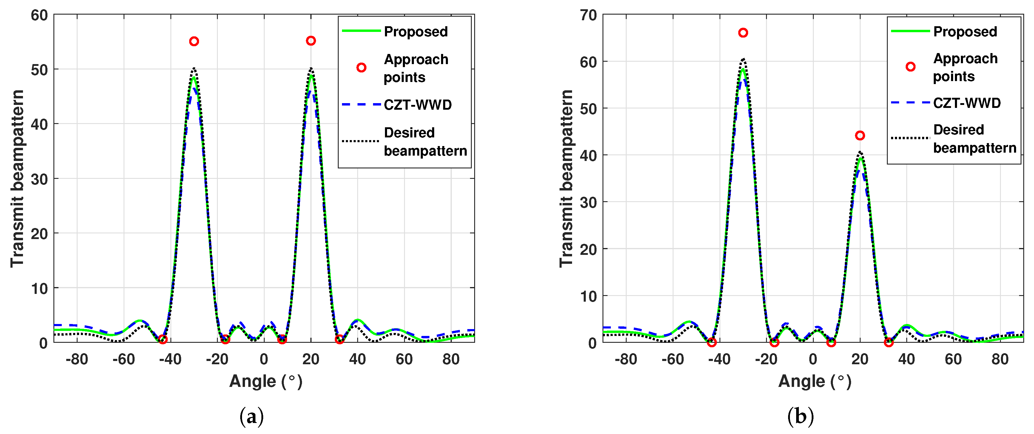
First, we show the transmit beampattern performance of the optimized waveforms. It is assumed that there are two beams pointing at and . For transmit beampattern performance comparison, the CZT-WWD in [18] is adopted. Though some other works have also considered the transmit waveform design for wideband MIMO radar [14,15,16,17], to the best of our knowledge, only CZT-WWD considered the transmit beampattern match rather than the space–frequency pattern match. Therefore, for transmit beampattern design, CZT-WWD is an “apple-to-apple” comparison. In Figure 1, the transmit beampattern results of optimized waveforms are shown. The matching points for the proposed method are calculated according to the analysis in Section 3.1. The desired beampattern for CZT-WWD is a liner combination of two phased-array beams. It can be seen that both methods can form the desired transmit beampattern and can adjust the power of each beam. However, the beams produced by the proposed method have a higher transmit gain, which may be because the proposed method focuses more on approximating the approach points rather than matching the entire desired beampattern.
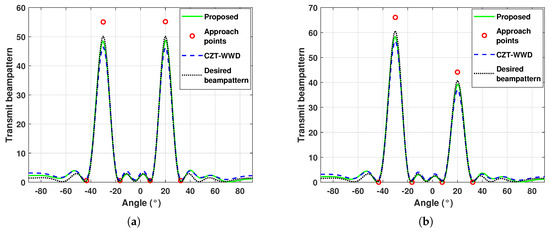
Figure 1.
Transmit beampattern performance comparison. (a) . (b) .
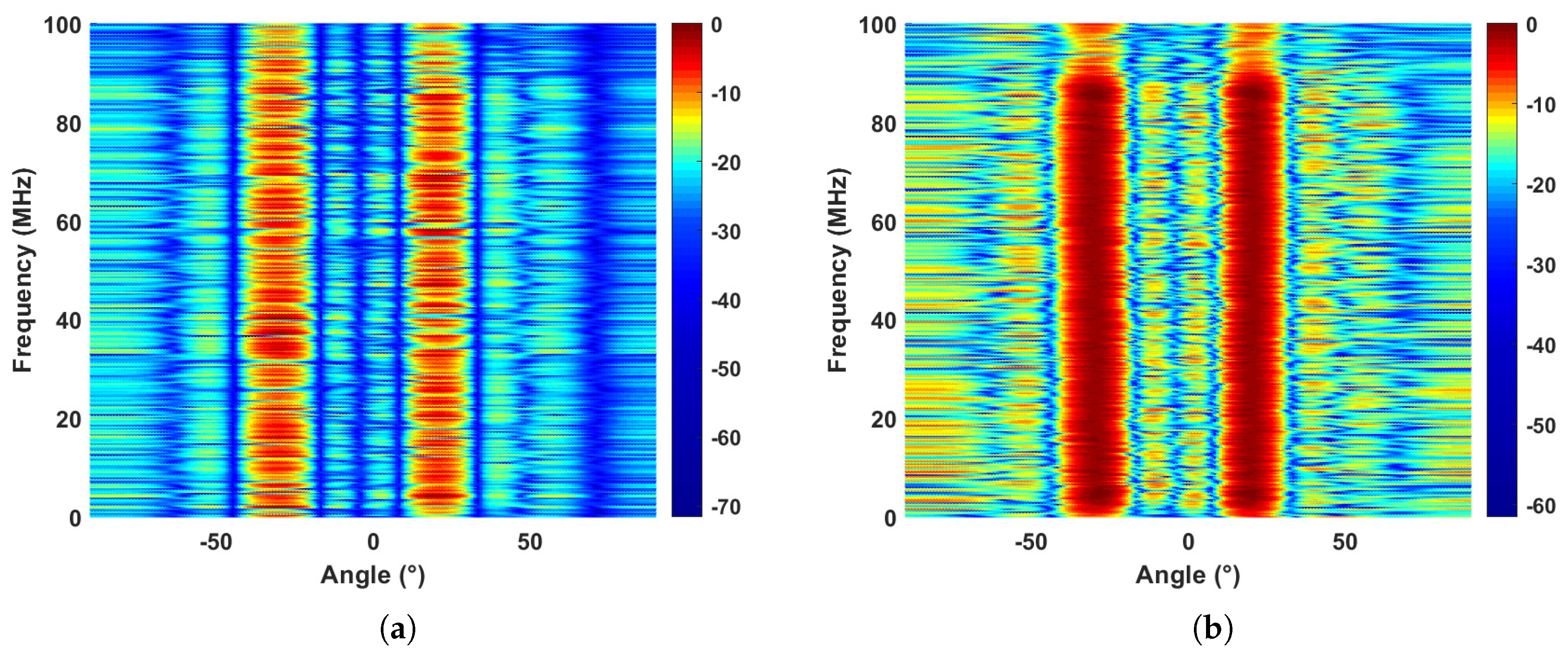
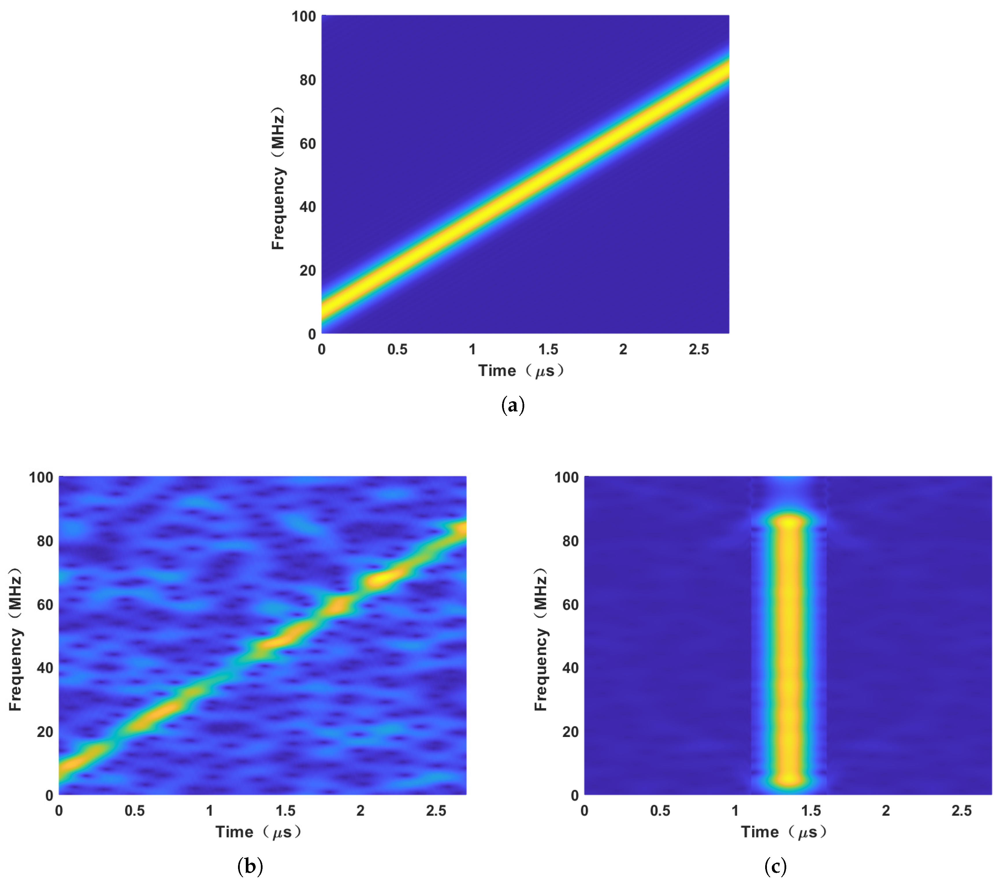
For AW design, the proposed method considers the matching for the reference signal frequency spectrums, including the amplitude and phase. However, CZT-WWD only considered the matching for the reference PSD. Therefore, the AWs produced by CZT-WWD cannot share all the TF characteristics of the reference signal. In Figure 2, we show the normalized space–frequency pattern corresponding to the result in Figure 1a, where the LFM signal with a chirp rate of is set as the reference signal, and the similarity parameter is set as 5. For CZT-WWD, the weight coefficient for the compromise between transmit beampattern and PSD matching is set as 1, and the reference PSD is the PSD of the above LFM signal. It can be seen that both methods can concentrate energy on the AWs of interest, and the proposed method has a lower sidelobe level. To verify the effectiveness of the similarity constraint, Figure 3 shows the TF distribution of the AWs at , corresponding to the result in Figure 2. It can be seen that the AWs produced by the proposed method share similar TF characteristics to the reference signal. Additionally, it is interesting that most of the energy of the AW produced by CZT-WWD is concentrated in the middle of the pulse, similar to an impulse function.
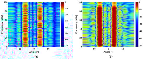
Figure 2.
The normalized space–frequency pattern corresponding to the result in Figure 1a. (a) The result of the proposed method. (b) The result of CZT-WWD.

Figure 3.
The TF distribution of AWs at . (a) The reference signal. (b) The result of the proposed method. (c) The result of CZT-WWD.
The motivation of our work is to realize de-chirp operation under the simultaneous multiple-beam case for wideband MIMO radar. Therefore, the de-chirp operation is implemented for the AWs produced by the proposed method. The de-chirp operation can be expressed as
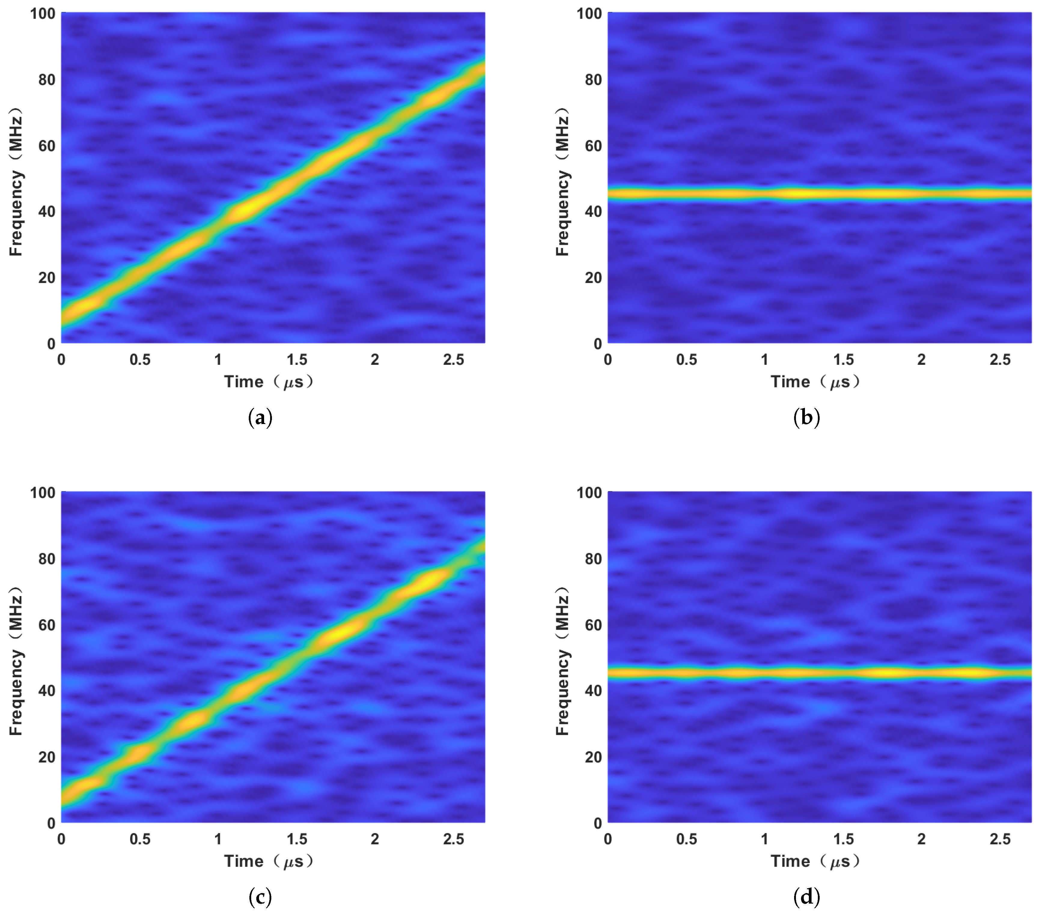
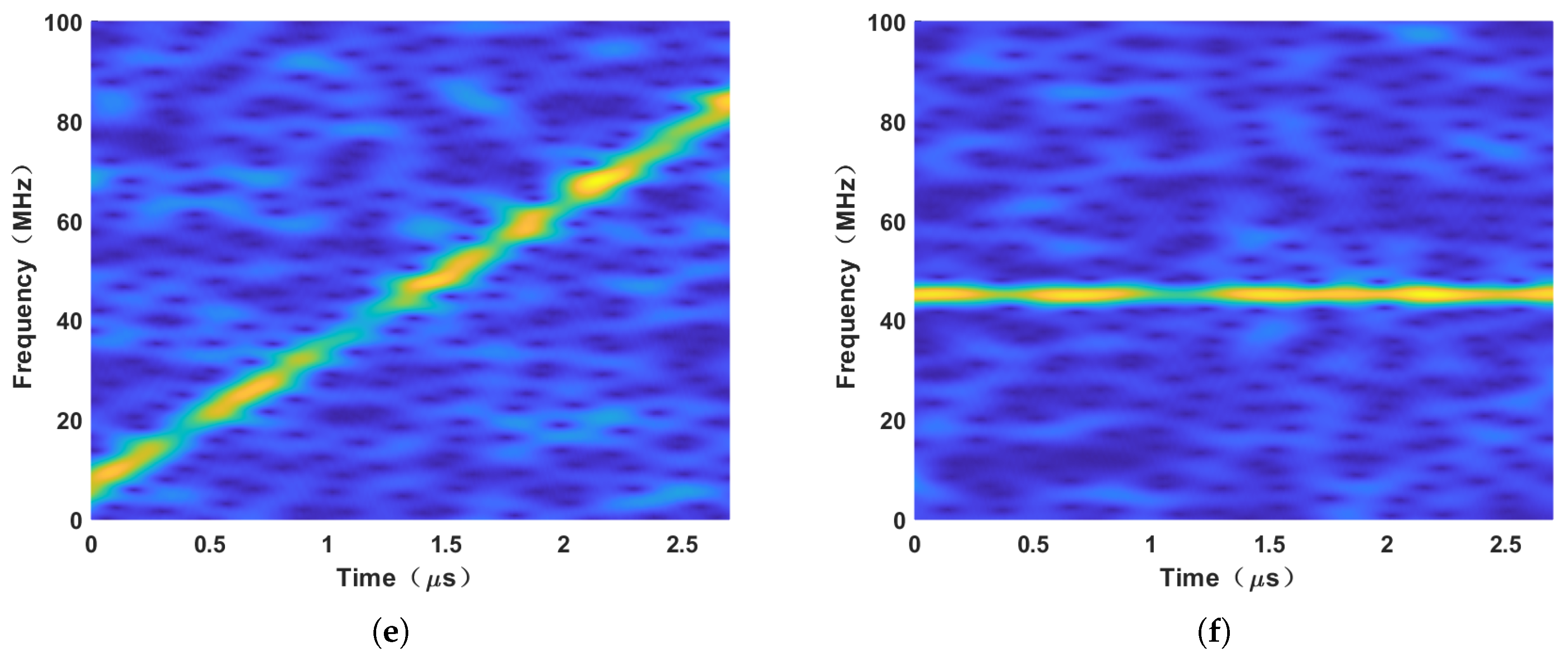
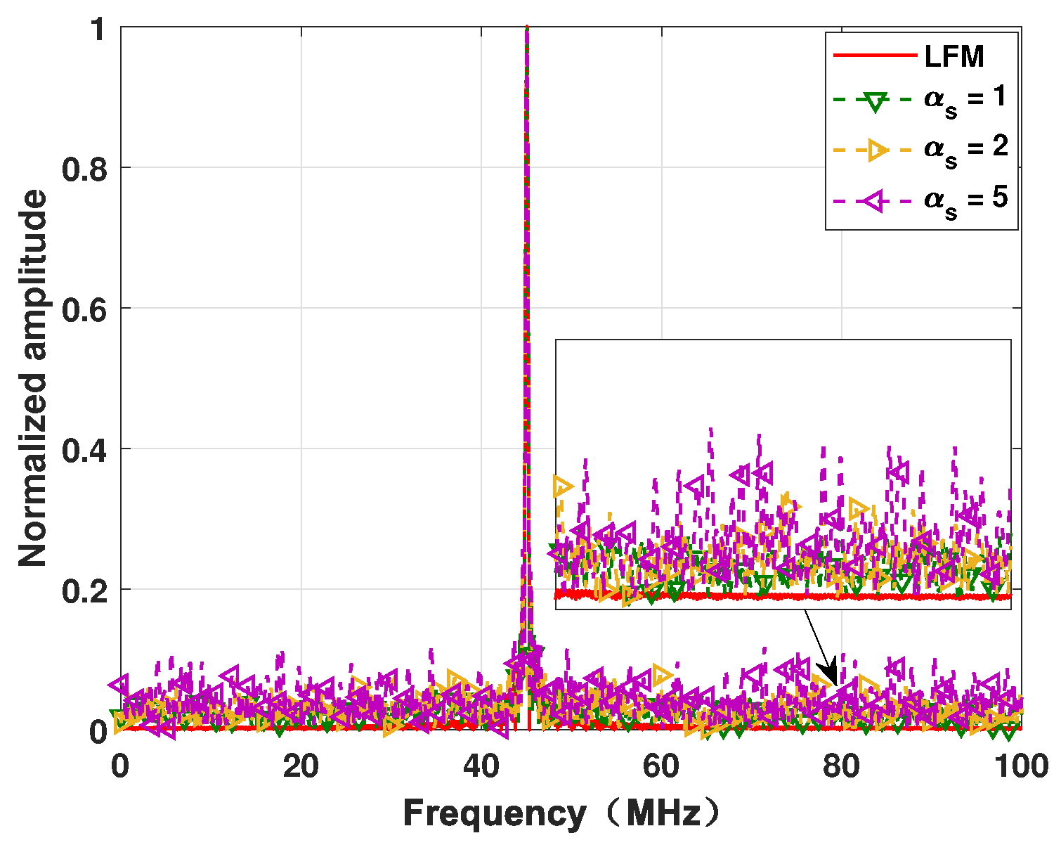
where is the inverse DFT of denoting the temporal expression of the AW at and denotes the discrete form of the above reference LFM signal after delay . Figure 4 shows the TF distribution of the AWs at when is set as 1, 2, and 5, and the corresponding TF distributions of the de-chirped signal are also shown. In Figure 4, the delay in the reference LFM signal is set as . Therefore, the ideal de-chirped signal will be a single-frequency signal at 45 MHz. From Figure 4, we can find that as the similarity parameter increases, the TF distribution of the AW gradually deviates from the reference signal. However, the de-chirped signals produced by (39) are nearly single-frequency signals, even if . Figure 5 shows the FFT result of the de-chirped signals, where the legend LFM denotes the FFT results of the reference LFM signal after the de-chirp operation. From Figure 5, it can be observed that though all AWs can form a single-frequency signal after the de-chirp operation, the frequency sidelobe level increases with the increase in . Therefore, a smaller similarity parameter means better target detection performance. It should be noted that the transmit gain is 47.23, 48.39, and 48.45, respectively, when the similarity parameter is 1, 2, and 5. This is because as the similarity parameter decreases, the feasible region of problem (29) is reduced and the transmit beam gain decreases. Therefore, the selection of the similarity parameter requires comprehensive consideration of the transmit gain and sidelobe level.
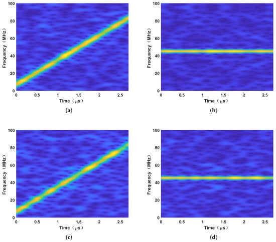

Figure 4.
The TF distributions of the AWs at and the TF distributions of corresponding de-chirped signals: (a) The AW when . (b) The de-chirped signal when . (c) The AW when . (d) The de-chirped signal when . (e) The AW when . (f) The de-chirped signal when .
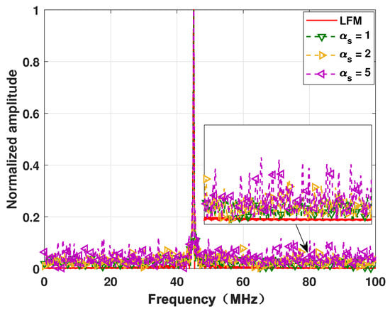
Figure 5.
The FFT result of the de-chirped signals.
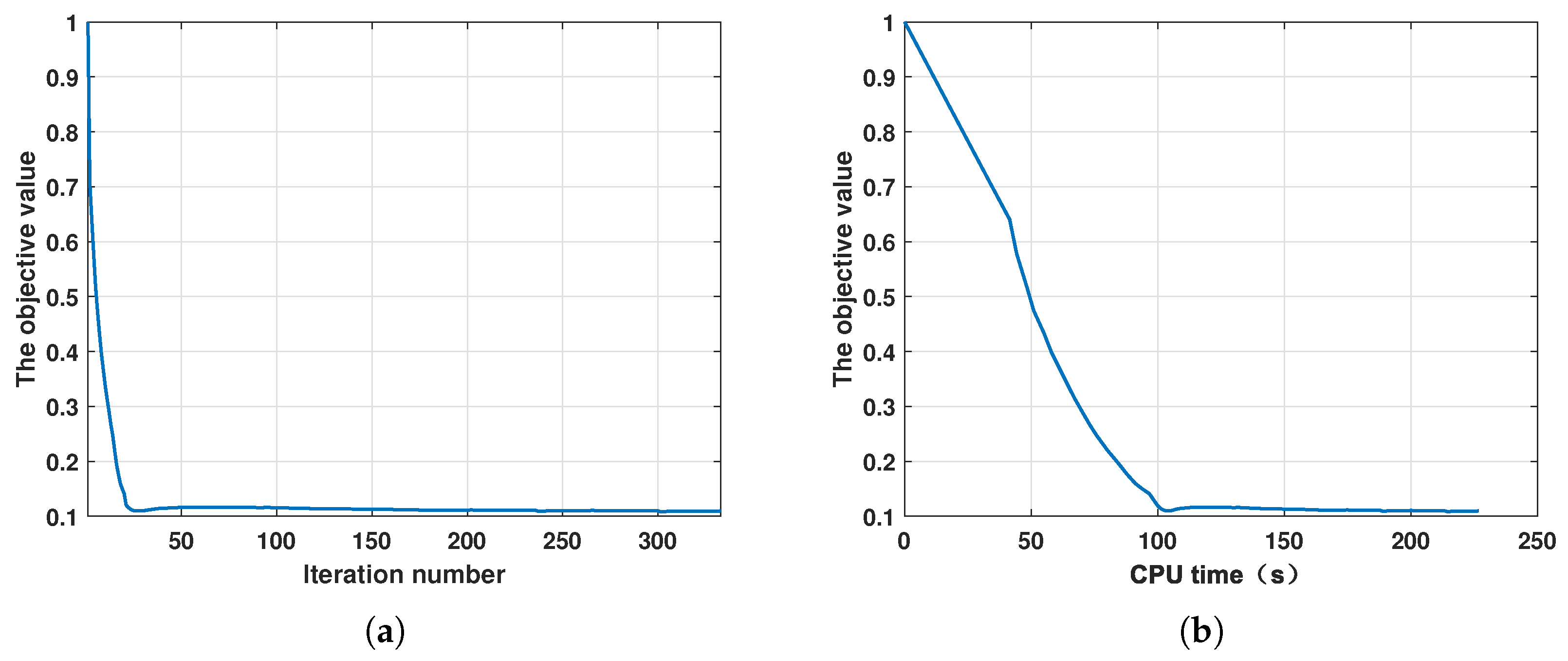
To empirically validate the convergence properties of the proposed method, we present the evolution of the objective function value with respect to both iteration number and computational time. It should be noted that the following curves were recorded when generating the results in Figure 1a. From Figure 6, it can be found that the proposed algorithm can still converge fast under wideband models.
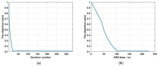
Figure 6.
versus: (a) iteration number and (b) time.
6. Discussion
In this section, we further explore the performance of the proposed method. There are three parts in this section. In the first part, we quantitatively describe the transmit beampattern performance and AW similarity of the generated waveform and investigate the influence of beam number on proposed algorithm feasibility and performance. The second part shows the suppression effect of receive beamforming on the mutual interference between AWs. An anti-ISRJ example using the proposed waveform is shown in the third part.
6.1. Quantitative Description of Waveform Performance
In this subsection, we quantitatively show the performance of the generated waveform. To evaluate the similarity of AWs, we define the following average normalized similarity:
To evaluate the beam gain of the transmit beampattern, we define the following average beam gain:
It should be noted that for the following results, is set as 2 and other radar parameters are the same as those in Table 1. Moreover, in order to evaluate the robustness of the proposed algorithm to the beam number, we show the results under different beam numbers and directions. Reviewing the constraints in problem (25), we consider the extreme situation that . In this extreme situation, the constraint regarding similarity can be ignored and the first two constraints regarding beampattern can be simplified as
It can be found that problem (25) has at least one feasible solution when [34]. According to the conclusion in this extreme situation, it can be inferred that each beam occupies three degrees of freedom in the proposed method. However, it is difficult to prove this conclusion in theory.
In Table 2, we show the quantitative results when . It can be found that the proposed waveform has better similarity performance than the CZT-WWD waveform. However, the beam gain performance of the proposed method becomes worse when the beam number is greater than three. In Table 3 and Table 4, we show the quantitative results of and , respectively. It can be observed that for , the beam gain performance of the proposed method becomes worse when the beam number is greater than four, and the beam gain performance of the proposed method is better than that of CZT-WWD for all considered beam numbers when . The above results can provide supporting evidence that the performance of the proposed algorithm is stable when .
Table 2.
The results when .
Table 3.
The results when .
Table 4.
The results when .
6.2. The Role of Receive Beamforming
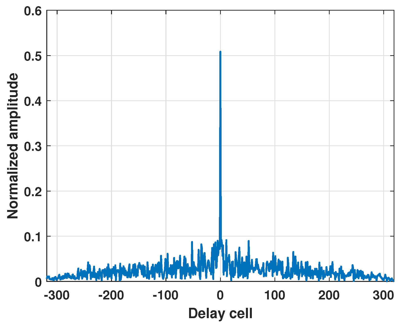
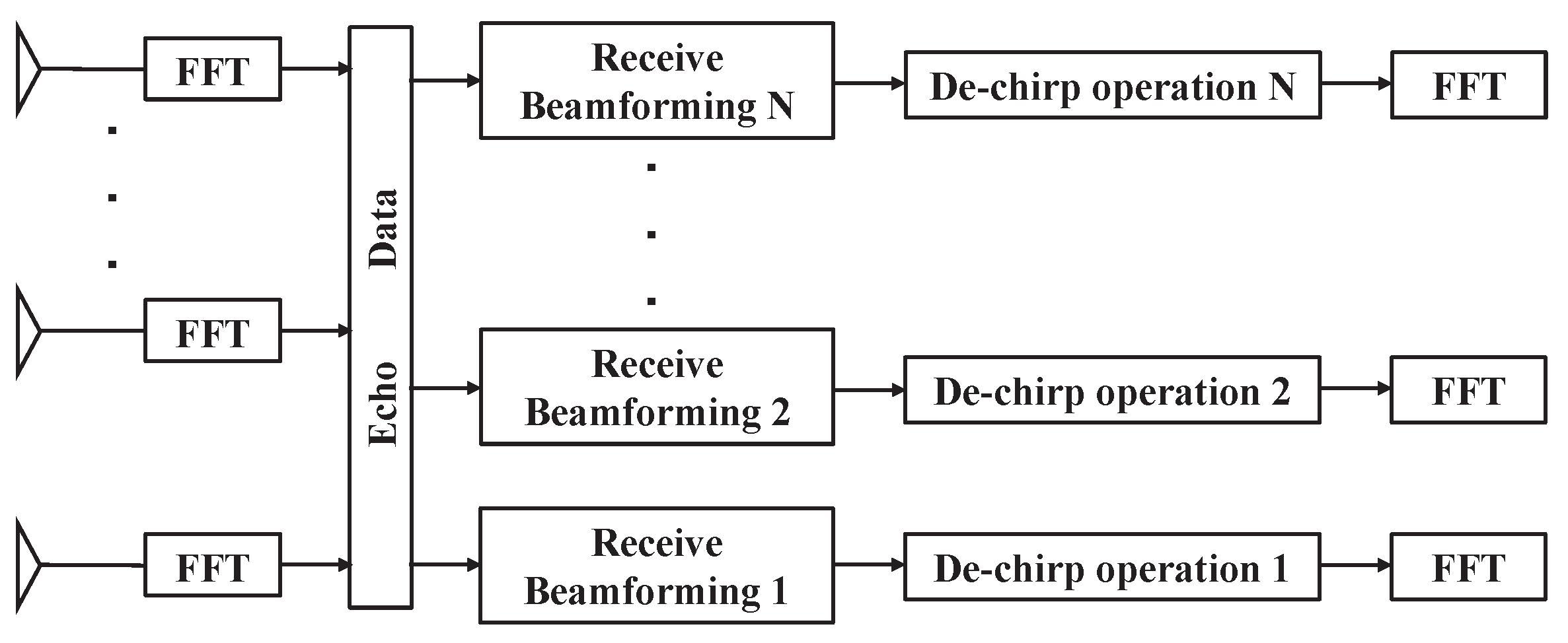
As shown in Figure 2, the AWs in different directions cover the same spectrum range, which inevitably causes interference between AWs. In Figure 7, we show the cross-correlation level between AWs, where the waveform results in Figure 2a are used. It can be found that the cross-correlation level at zero delay cell is too high to be used. However, it can be noticed that the AWs can be separated in the spatial domain. Therefore, the signal processing strategy in Figure 8 is adopted, where the receive beamforming is performed first and then the de-chirp and FFT operations follow to realize pulse compression (PC).

Figure 7.
The cross-correlation level between AWs.
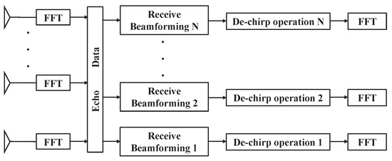
Figure 8.
The adopted signal processing strategy.
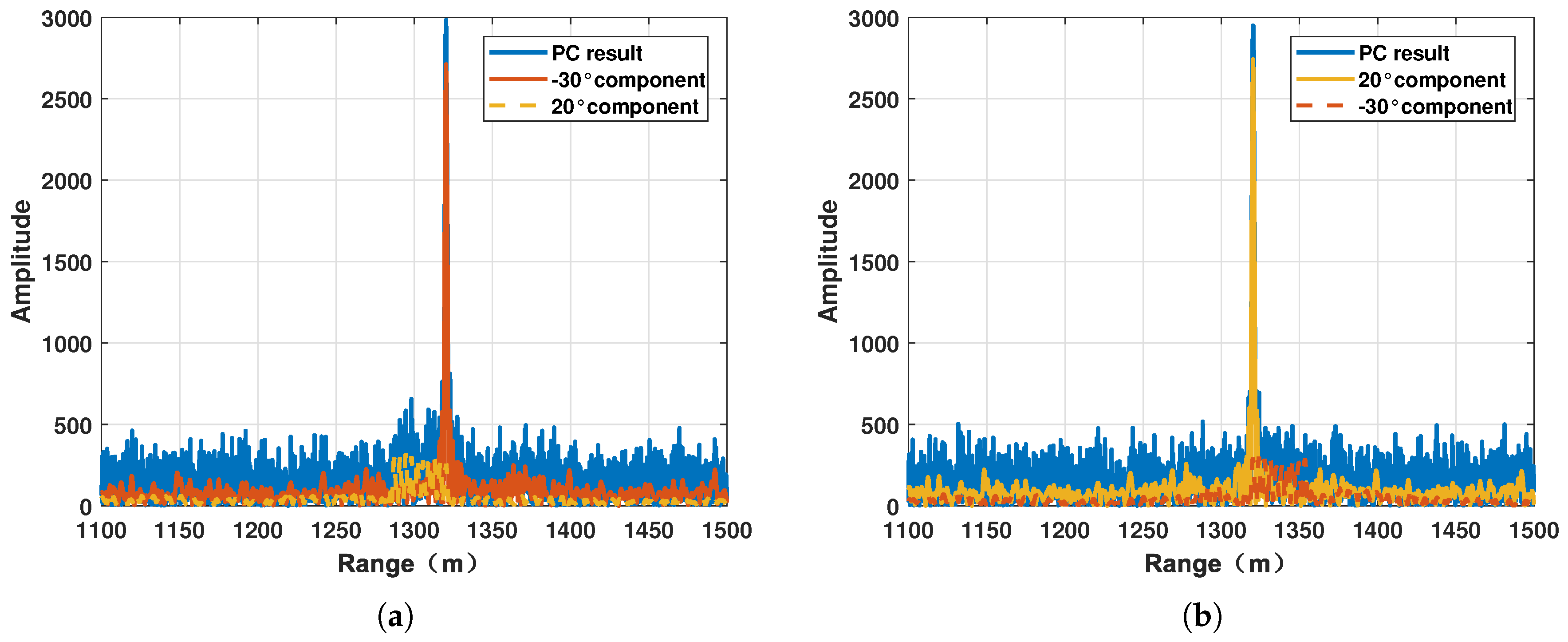
In order to more realistically demonstrate the effect of receiving beamforming, in the following simulations, we assume that there are two targets located at and 20° respectively, and the ranges of the two targets are both 1320 m and the input signal-to-noise ratios (SNRs) are both 0 dB. In Figure 9, the receive beamforming output and the components of echoes from different directions are shown. It can be seen that after receive beamforming, the components of echoes from undesired directions have been suppressed at the noise level. In Figure 10, we shown the PC results of the receive beamforming output and the PC results of the components of echoes from different directions. It can be seen that the echo component from the desired direction can form a peak, while the echo component from the undesired direction has been suppressed below the noise level. The above simulation results verify that the receive beamforming operation can suppress the mutual interference between AWs. To achieve a better suppression effect, adaptive beamforming technology can be further adopted here.
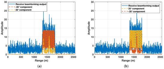
Figure 9.
The receive beamforming output. (a) The receive beamforming output at . (b) The receive beamforming output at 20°.
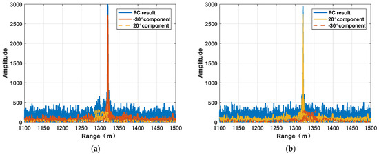
Figure 10.
The PC results. (a) The PC results of receive beamforming output. (b) The PC results of 20° receive beamforming output.
6.3. An Anti-ISRJ Example
In this subsection, an anti-ISRJ example is presented to show the anti-jamming performance of the waveform generated by the proposed method. The radar parameters are the same as those in Table 1, and the radar receive end shares the same array as the transmit end. For the mechanism of ISRJ, readers can refer to reference [27]. In this example, the parameters of ISRJs and targets are shown in Table 5.
Table 5.
The parameters of ISRJs and targets.
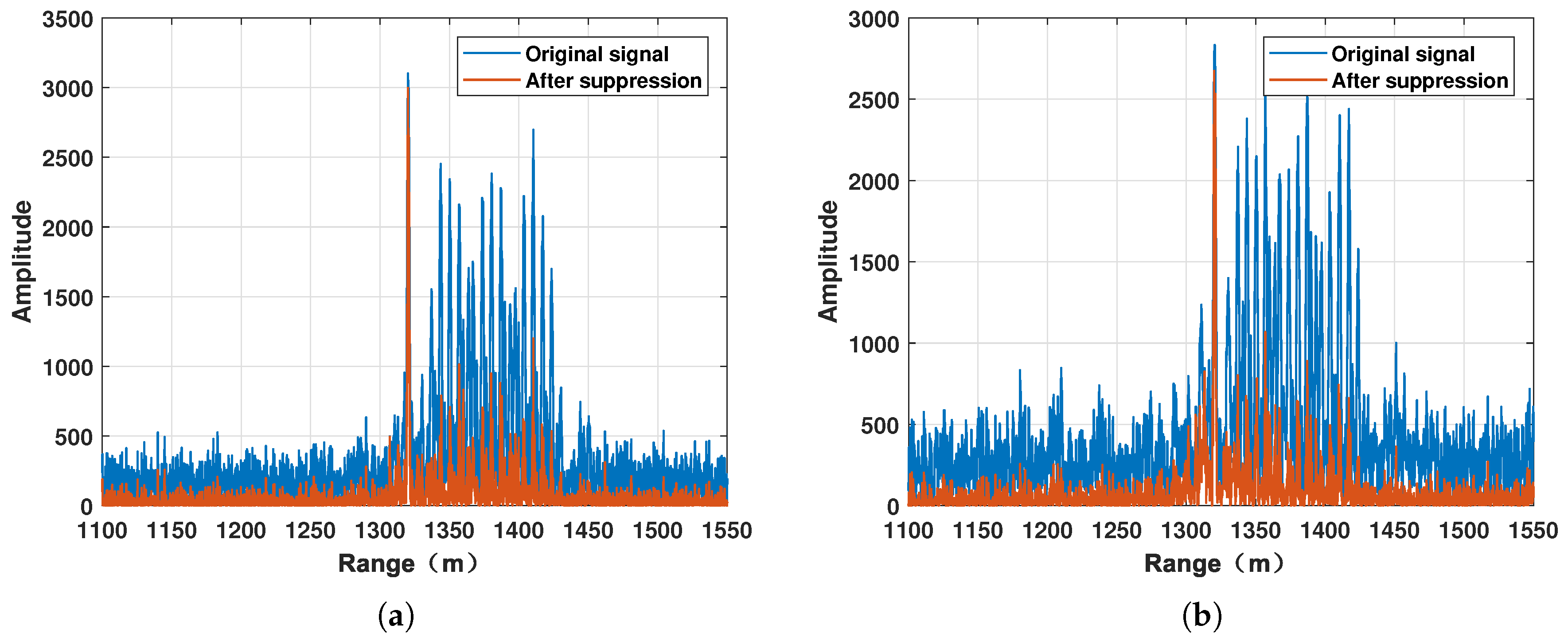
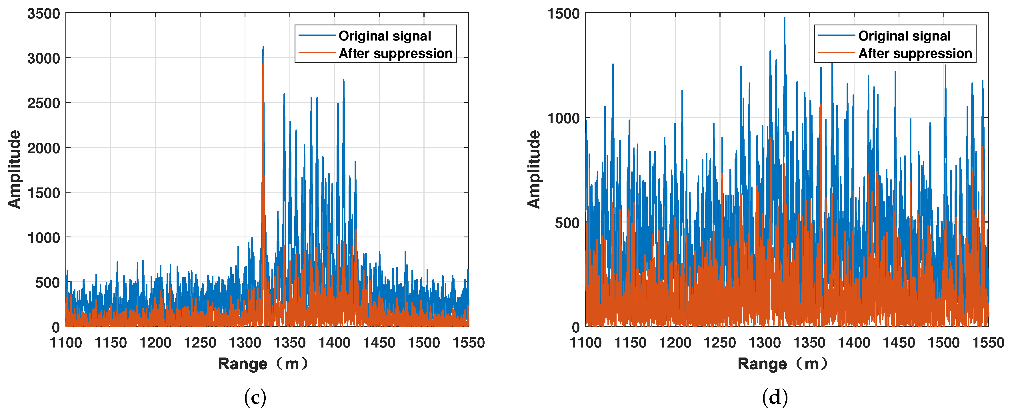
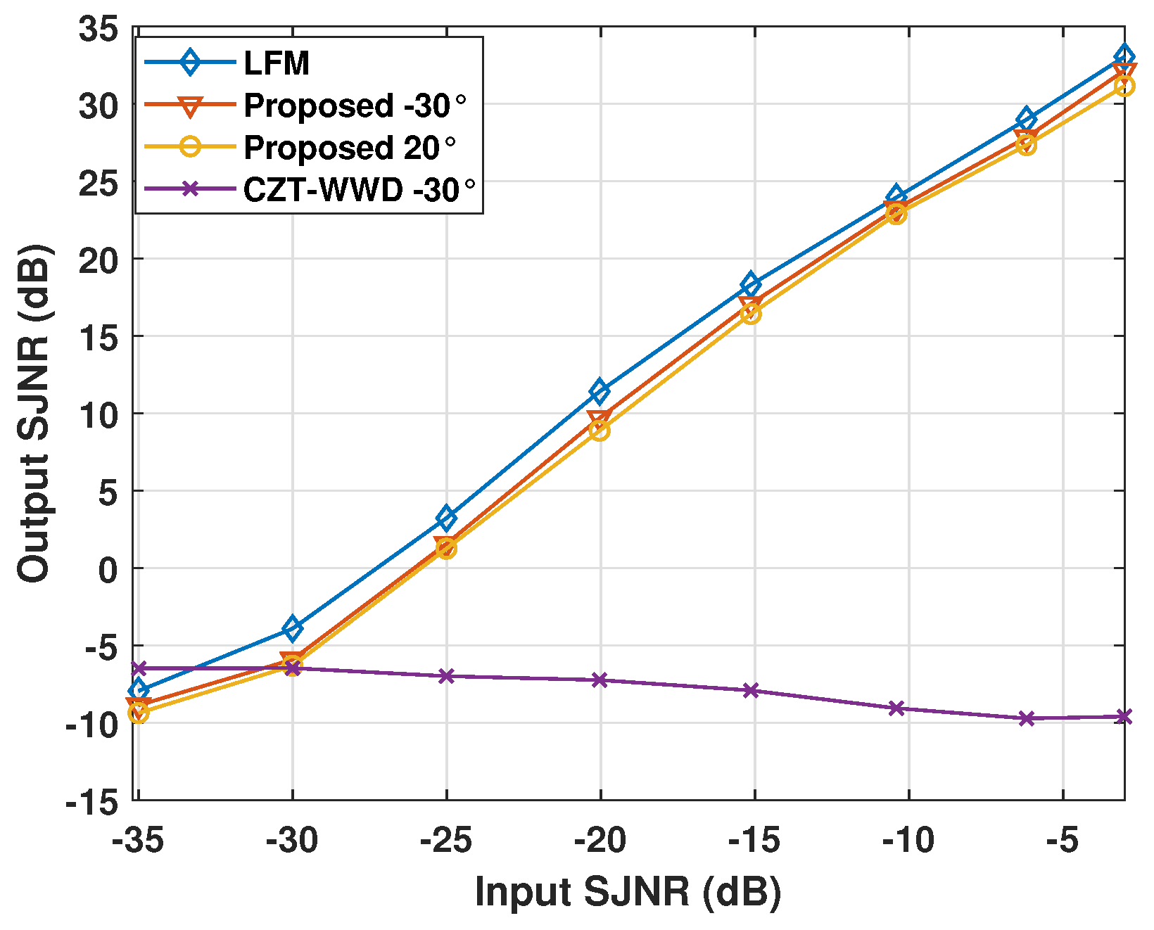
It should be noted that the waveform in the previous subsection is adopted here. Therefore, there are two targets located at and 20°, respectively, and they are protected by ISRJs. The anti-ISRJ method in [30] is adopted, which utilizes the de-chirped signal of LFM. In Figure 11, we show the ISRJ suppression results corresponding to the waveforms generated by different methods. For the waveforms generated by the proposed method and CZT-WWD, the signal processing strategy in Figure 8 is adopted. The reference LFM signal forms a single beam at , and only the receive beamforming output at is considered. Because the ISRJ suppression results corresponding to the CZT-WWD waveform are chaotic, we only show the ISRJ suppression results at . From Figure 11, it can be seen that both the AWs of the proposed method share a similar anti-ISRJ performance to the LFM signal, but the waveform generated by CZT-WWD does not have similar capabilities. Essentially, this is because the waveform generated by CZT-WWD cannot undergo the de-chirp operation. In Figure 12, we show the output signal-to-jamming-plus-noise ratio (SJNR) versus the input SJNR for different waveforms. Each curve is the average result of 200 random trials. It can be found that the proposed waveform has a similar output SJNR performance to the reference LFM signal. Because the waveform generated by CZT-WWD cannot share the TF characteristic of LFM, it can be seen that the output SJNR of CZT-WWD waveform is unconventional and relatively stable.
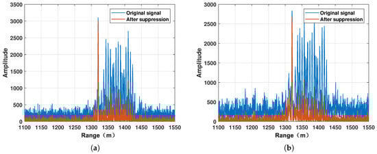
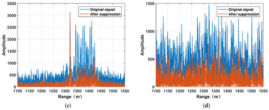
Figure 11.
The ISRJ suppression results. (a) The reference LFM signal. (b) The AW at of the proposed waveform. (c) The AW at 20° of the proposed waveform. (d) The AW at of the CZT-WWD waveform.
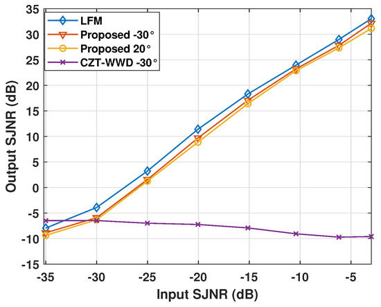
Figure 12.
The output SJNR versus the input SJNR.
7. Conclusions
In this paper, we consider the joint design of transmit beampattern and AW similarity for wideband MIMO radar. Compact formulations of the transmit beampattern and AW are constructed. Based on the proposed signal model, an optimization model for joint design is formulated under the CM constraint, and an existing algorithm is extended to the wideband case. The motivation of this paper is to design AWs that can share the TF characteristics of LFM and can realize the de-chirp operation. Simulation results demonstrate that the proposed method can generate the desired multi-beam beampattern and the AWs in mainlobe directions can perform the de-chirp operation.
Author Contributions
Conceptualization, H.Z.; methodology, H.Z.; software, H.Z. validation, H.Z. and S.W.; investigation, H.Z. and J.Y.; writing—original draft preparation, H.Z.; writing—review and editing, H.Z. and X.Z.; supervision, H.Z. All authors have read and agreed to the published version of the manuscript.
Funding
This work was supported by the National Natural Science Foundation of China under grants 62361046, 62461047 and 62371264, the Natural Science Foundation of Inner Mongolia Autonomous Region of China under grants 2023QN06003 and 2021JQ07, the Young Talents of Science and Technology in Universities of Inner Mongolia Autonomous Region under grant NJYT22109, the Training Plan for Young Innovative of Grassland Talents Project in Inner Mongolia Autonomous Region under grant Q2022003, the Innovation Capability Support Program of Shaanxi under grant 2023KJXX-015, and the Science and Technology Project of Henan Province under grant 252102210246.
Data Availability Statement
The original contributions presented in the study are included in the article; further inquiries can be directed to the corresponding author.
Conflicts of Interest
The authors declare no conflicts of interest.
References
- Fuhrmann, D.; San Antonio, G. Transmit beamforming for MIMO radar systems using partial signal correlation. In Proceedings of the Conference Record of the Thirty-Eighth Asilomar Conference on Signals, Systems and Computers, Pacific Grove, CA, USA, 7–10 November 2004; Volume 1, pp. 295–299. [Google Scholar] [CrossRef]
- Fishler, E.; Haimovich, A.; Blum, R.; Cimini, R.; Chizhik, D.; Valenzuela, R. Performance of MIMO radar systems: Advantages of angular diversity. In Proceedings of the Conference Record of the Thirty-Eighth Asilomar Conference on Signals, Systems and Computers, Pacific Grove, CA, USA, 7–10 November 2004; Volume 1, pp. 305–309. [Google Scholar] [CrossRef]
- Robey, F.; Coutts, S.; Weikle, D.; McHarg, J.; Cuomo, K. MIMO radar theory and experimental results. In Proceedings of the Conference Record of the Thirty-Eighth Asilomar Conference on Signals, Systems and Computers, Pacific Grove, CA, USA, 7–10 November 2004; Volume 1, pp. 300–304. [Google Scholar] [CrossRef]
- Stoica, P.; Li, J.; Xie, Y. On Probing Signal Design for MIMO Radar. IEEE Trans. Signal Process. 2007, 55, 4151–4161. [Google Scholar] [CrossRef]
- Stoica, P.; Li, J.; Zhu, X. Waveform Synthesis for Diversity-Based Transmit Beampattern Design. IEEE Trans. Signal Process. 2008, 56, 2593–2598. [Google Scholar] [CrossRef]
- Yu, X.; Cui, G.; Zhang, T.; Kong, L. Constrained transmit beampattern design for colocated MIMO radar. Signal Process. 2018, 144, 145–154. [Google Scholar] [CrossRef]
- Li, H.; Zhao, Y.; Cheng, Z.; Feng, D. Correlated LFM Waveform Set Design for MIMO Radar Transmit Beampattern. IEEE Geosci. Remote Sens. Lett. 2017, 14, 329–333. [Google Scholar] [CrossRef]
- Zhou, S.; Lu, J.; Varshney, P.K.; Wang, J.; Liu, H. Colocated MIMO radar waveform optimization with receive beamforming. Digit. Signal Process. 2019, 98, 102635. [Google Scholar] [CrossRef]
- Wang, Y.C.; Xu, W.; Liu, H.; Luo, Z.Q. On the Design of Constant Modulus Probing Signals for MIMO Radar. IEEE Trans. Signal Process. 2012, 60, 4432–4438. [Google Scholar] [CrossRef]
- Wang, J.; Wang, Y. On the Design of Constant Modulus Probing Waveforms with Good Correlation Properties for MIMO Radar via Consensus-ADMM Approach. IEEE Trans. Signal Process. 2019, 67, 4317–4332. [Google Scholar] [CrossRef]
- Cheng, Z.; He, Z.; Zhang, S.; Jian, L. Constant Modulus Waveform Design for MIMO Radar Transmit Beampattern. IEEE Trans. Signal Process. 2017, 65, 4912–4923. [Google Scholar] [CrossRef]
- Aldayel, O.; Monga, V.; Rangaswamy, M. Tractable Transmit MIMO Beampattern Design Under a Constant Modulus Constraint. IEEE Trans. Signal Process. 2017, 65, 2588–2599. [Google Scholar] [CrossRef]
- Imani, S.; Nayebi, M.M.; Ghorashi, S. Transmit Signal Design in Co-located MIMO Radar Without Covariance Matrix Optimization. IEEE Trans. Aerosp. Electron. Syst. 2017, 53, 2178–2186. [Google Scholar] [CrossRef]
- Mccormick, P.M.; Blunt, S.D.; Metcalf, J.G. Wideband MIMO Frequency Modulated Emission Design with Space-Frequency Nulling. IEEE J. Sel. Top. Signal Process. 2016, 11, 363–378. [Google Scholar] [CrossRef]
- Yu, X.; Cui, G.; Yang, J.; Kong, L.; Li, J. Wideband MIMO Radar Waveform Design. IEEE Trans. Signal Process. 2019, 67, 3487–3501. [Google Scholar] [CrossRef]
- He, H.; Stoica, P.; Li, J. Wideband MIMO Systems: Signal Design for Transmit Beampattern Synthesis. IEEE Trans. Signal Process. 2011, 59, 618–628. [Google Scholar] [CrossRef]
- Tang, Y.; Zhang, Y.D.; Amin, M.G.; Sheng, W. Wideband Multiple-Input Multiple-Output Radar Waveform Design with Low Peak-to-Average Ratio Constraint; IET: Washington, DC, USA, 2016. [Google Scholar]
- Liu, H.; Wang, X.; Jiu, B.; Yan, J.; Wu, M.; Bao, Z. Wideband MIMO Radar Waveform Design for Multiple Target Imaging. IEEE Sens. J. 2016, 16, 8545–8556. [Google Scholar] [CrossRef]
- Friedlander, B. On Transmit Beamforming for MIMO Radar. IEEE Trans. Aerosp. Electron. Syst. 2012, 48, 3376–3388. [Google Scholar] [CrossRef]
- Shi, J.; Bo, J.; Liu, H.; Ming, F.; Yan, J. Transmit design for airborne MIMO radar based on prior information. Signal Process. 2016, 128, 521–530. [Google Scholar] [CrossRef]
- Yan, J.; Liu, H.; Jiu, B.; Chen, B.; Liu, Z.; Bao, Z. Simultaneous Multibeam Resource Allocation Scheme for Multiple Target Tracking. IEEE Trans. Signal Process. 2015, 63, 3110–3122. [Google Scholar] [CrossRef]
- Yan, J.; Jiu, B.; Liu, H.; Chen, B.; Bao, Z. Prior Knowledge-Based Simultaneous Multibeam Power Allocation Algorithm for Cognitive Multiple Targets Tracking in Clutter. IEEE Trans. Signal Process. 2015, 63, 512–527. [Google Scholar] [CrossRef]
- Zhou, S.; Liu, H.; Hongtao Su, H.Z. Doppler sensitivity of MIMO radar waveforms. IEEE Trans. Aerosp. Electron. Syst. 2016, 52, 2091–2110. [Google Scholar] [CrossRef]
- Zheng, H.; Jiu, B.; Li, K.; Liu, H. Joint Design of the Transmit Beampattern and Angular Waveform for Colocated MIMO Radar under a Constant Modulus Constraint. Remote Sens. 2021, 13, 3392. [Google Scholar] [CrossRef]
- Lazecky, M.; Hlavacova, I.; Bakon, M.; Sousa, J.J.; Perissin, D.; Patricio, G. Bridge Displacements Monitoring Using Space-Borne X-Band SAR Interferometry. IEEE J. Sel. Top. Appl. Earth Obs. Remote Sens. 2017, 10, 205–210. [Google Scholar] [CrossRef]
- Zhou, X.; Chong, J.; Yang, X.; Li, W.; Guo, X. Ocean Surface Wind Retrieval Using SMAP L-Band SAR. IEEE J. Sel. Top. Appl. Earth Obs. Remote Sens. 2017, 10, 65–74. [Google Scholar] [CrossRef]
- Wang, X.S.; Liu, J.C.; Zhang, W.M.; Qixiang, F.U.; Liu, Z.; Xie, X.X. Mathematic principles of interrupted-sampling repeater jamming (ISRJ). Sci. China 2007, 50, 113–123. [Google Scholar] [CrossRef]
- Gong, S.; Wei, X.; Li, X. ECCM scheme against interrupted sampling repeater jammer based on time-frequency analysis. J. Syst. Eng. Electron. 2014, 25, 996–1003. [Google Scholar] [CrossRef]
- Chen, J.; Wu, W.; Xu, S.; Chen, P.; Zou, J.W. A Band Pass Filter Design against Interrupted-Sampling Repeater Jamming based on Time-Frequency Analysis. IET Radar Sonar Navig. 2019, 13. [Google Scholar] [CrossRef]
- Yuan, H.; Wang, C.; Li, X.; An, L. A Method against Interrupted-Sampling Repeater Jamming Based on Energy Function Detection and Band-Pass Filtering. Int. J. Antennas Propag. 2017, 2017, 6759169. [Google Scholar] [CrossRef]
- Wang, Z.; Li, J.; Yu, W.; Luo, Y.; Zhao, Y.; Yu, Z. Energy function-guided histogram analysis for interrupted sampling repeater jamming suppression. Electron. Lett. 2023, 59, e12778. [Google Scholar] [CrossRef]
- Meng, Y.; Yu, L.; Wei, Y. Interrupted Sampling Repeater Jamming Suppression Based on Time-frequency Segmentation Network and Target Signal Reconstruction. In Proceedings of the 2023 IEEE International Radar Conference (RADAR), Sydney, Australia, 6–10 November 2023; pp. 1–5. [Google Scholar] [CrossRef]
- Duan, L.; Du, S.; Quan, Y.; Lv, Q.; Li, S.; Xing, M. Interference Countermeasure System Based on Time–Frequency Domain Characteristics. IEEE J. Miniat. Air Space Syst. 2023, 4, 76–84. [Google Scholar] [CrossRef]
- Trees, H.L.V. Optimum Array Processing; John Wiley & Sons, Ltd.: Hoboken, NJ, USA, 2002; Chapter 7; pp. 710–916. [Google Scholar] [CrossRef]

Disclaimer/Publisher’s Note: The statements, opinions and data contained in all publications are solely those of the individual author(s) and contributor(s) and not of MDPI and/or the editor(s). MDPI and/or the editor(s) disclaim responsibility for any injury to people or property resulting from any ideas, methods, instructions or products referred to in the content. |
© 2025 by the authors. Licensee MDPI, Basel, Switzerland. This article is an open access article distributed under the terms and conditions of the Creative Commons Attribution (CC BY) license (https://creativecommons.org/licenses/by/4.0/).