
Super Resolution Reconstruction of Mars Thermal Infrared Remote Sensing Images Integrating Multi-Source Data


Abstract
1. Introduction
2. Related Works
2.1. Reconstruction-Based Method
2.2. Learning-Based Method
3. Methods
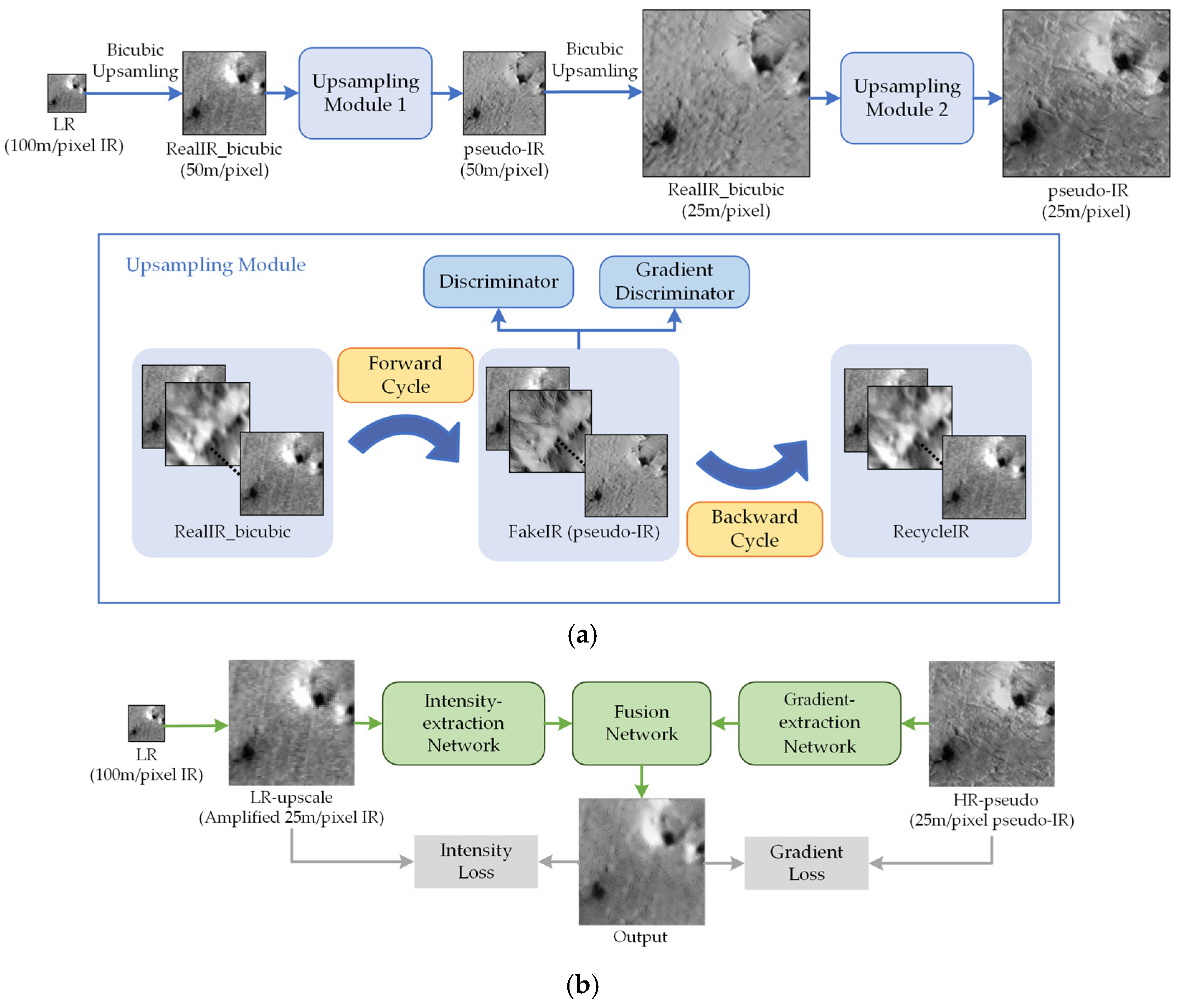
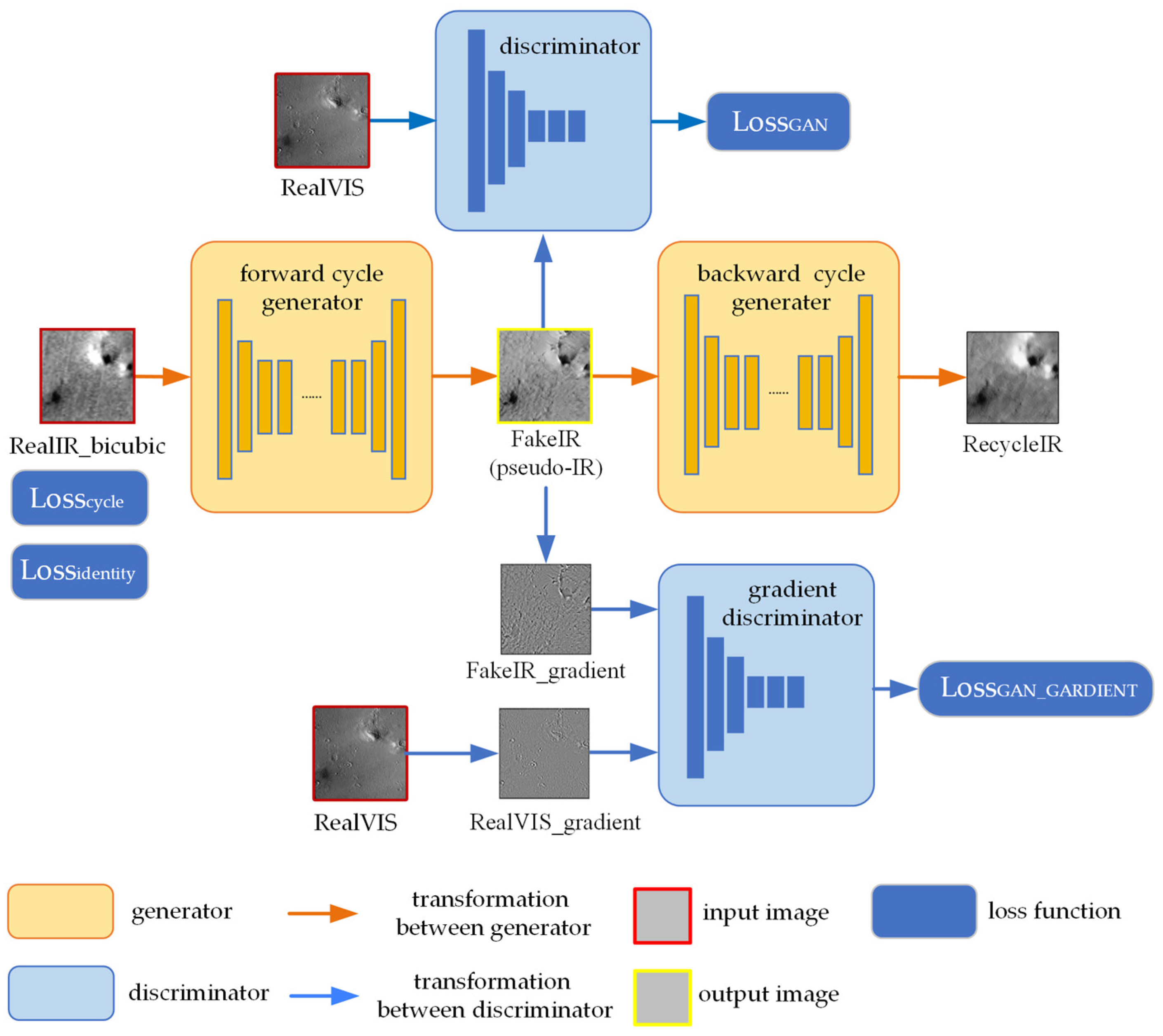
3.1. Super-Resolution Reconstruction of Thermal Infrared Images with Visible Light Texture Reference
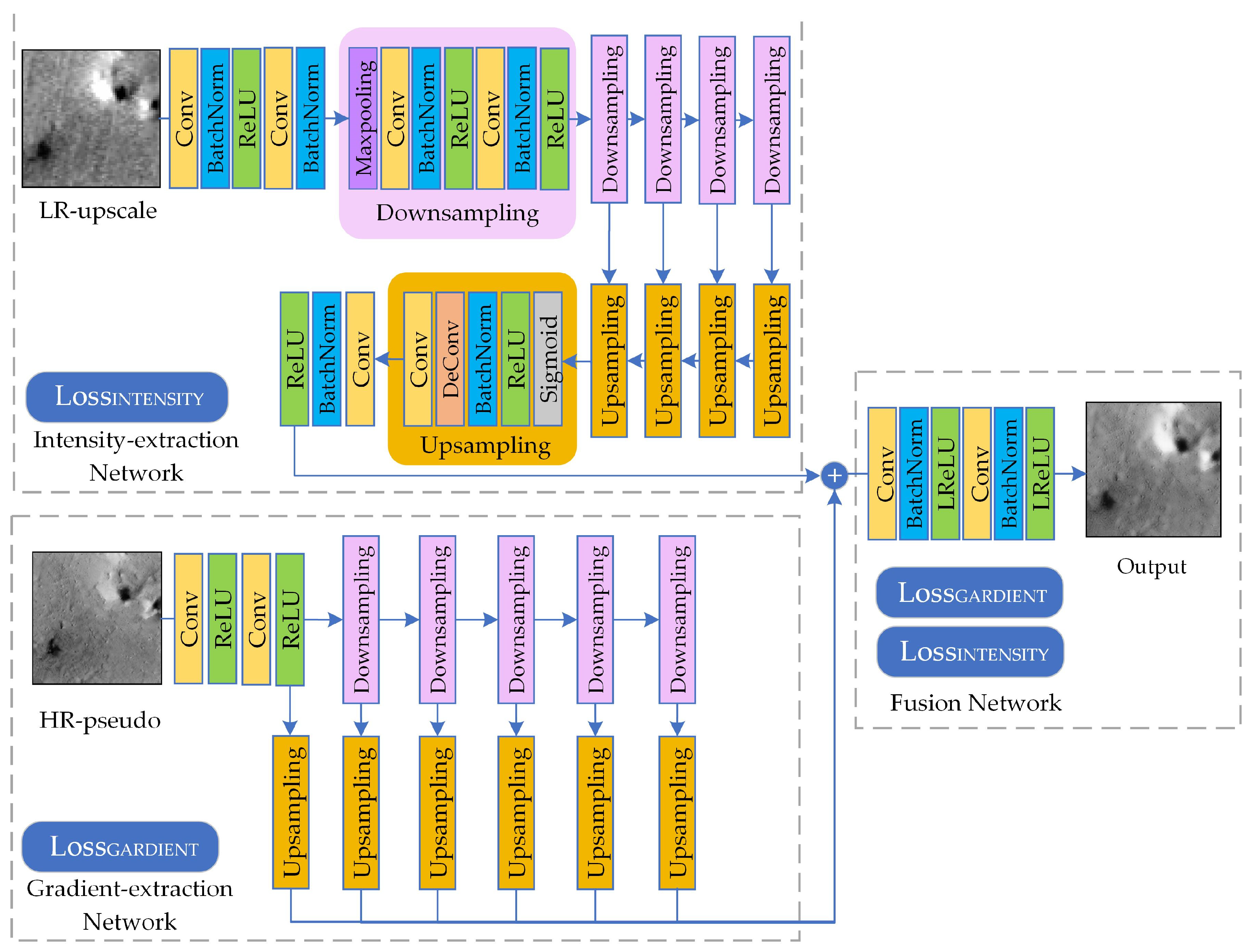
3.2. Consistency Constraints on Thermal Radiation Flux
3.2.1. Intensity-Extraction Network
3.2.2. Gradient-Extraction Network
3.2.3. Fusion Network
4. Experiment
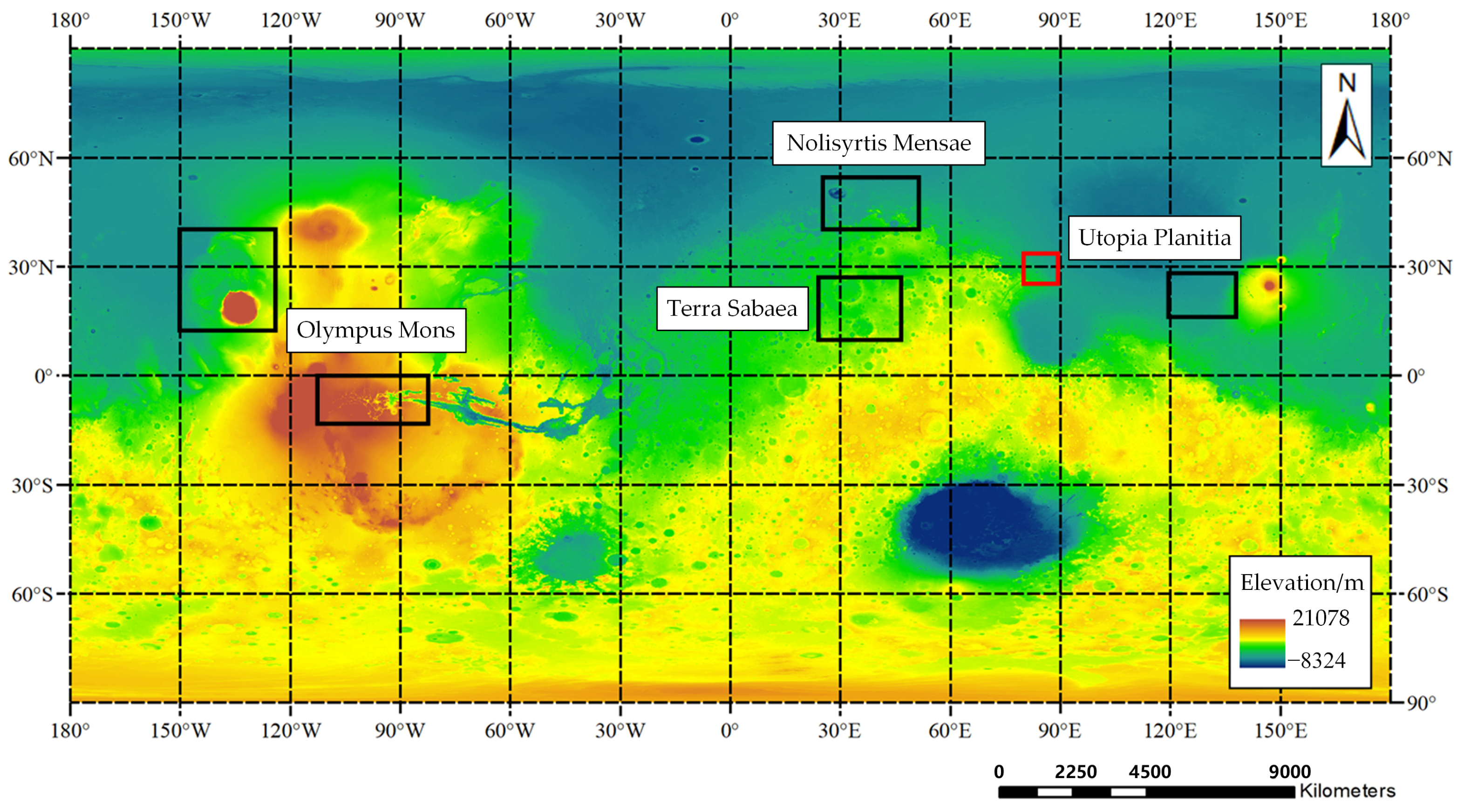
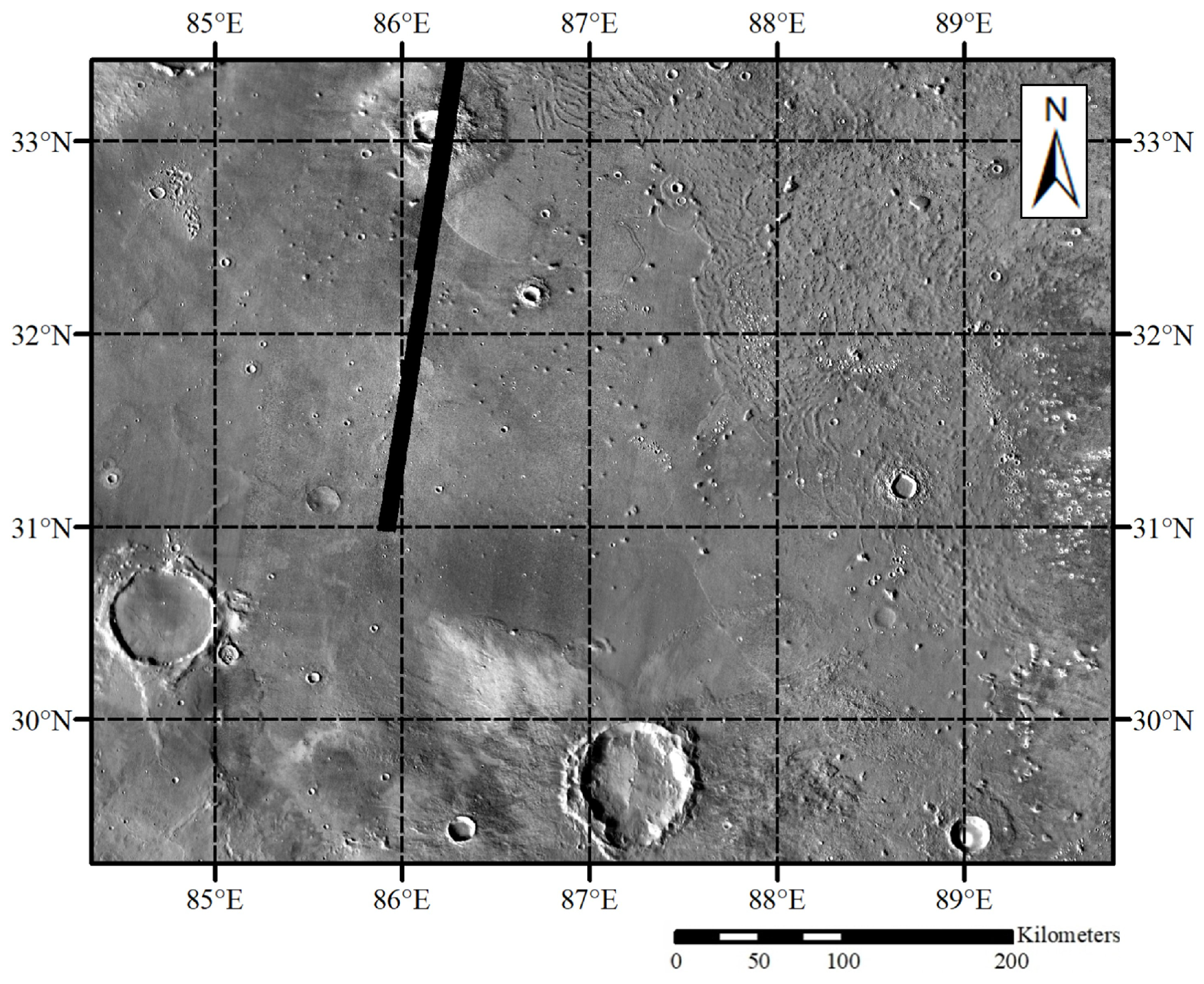
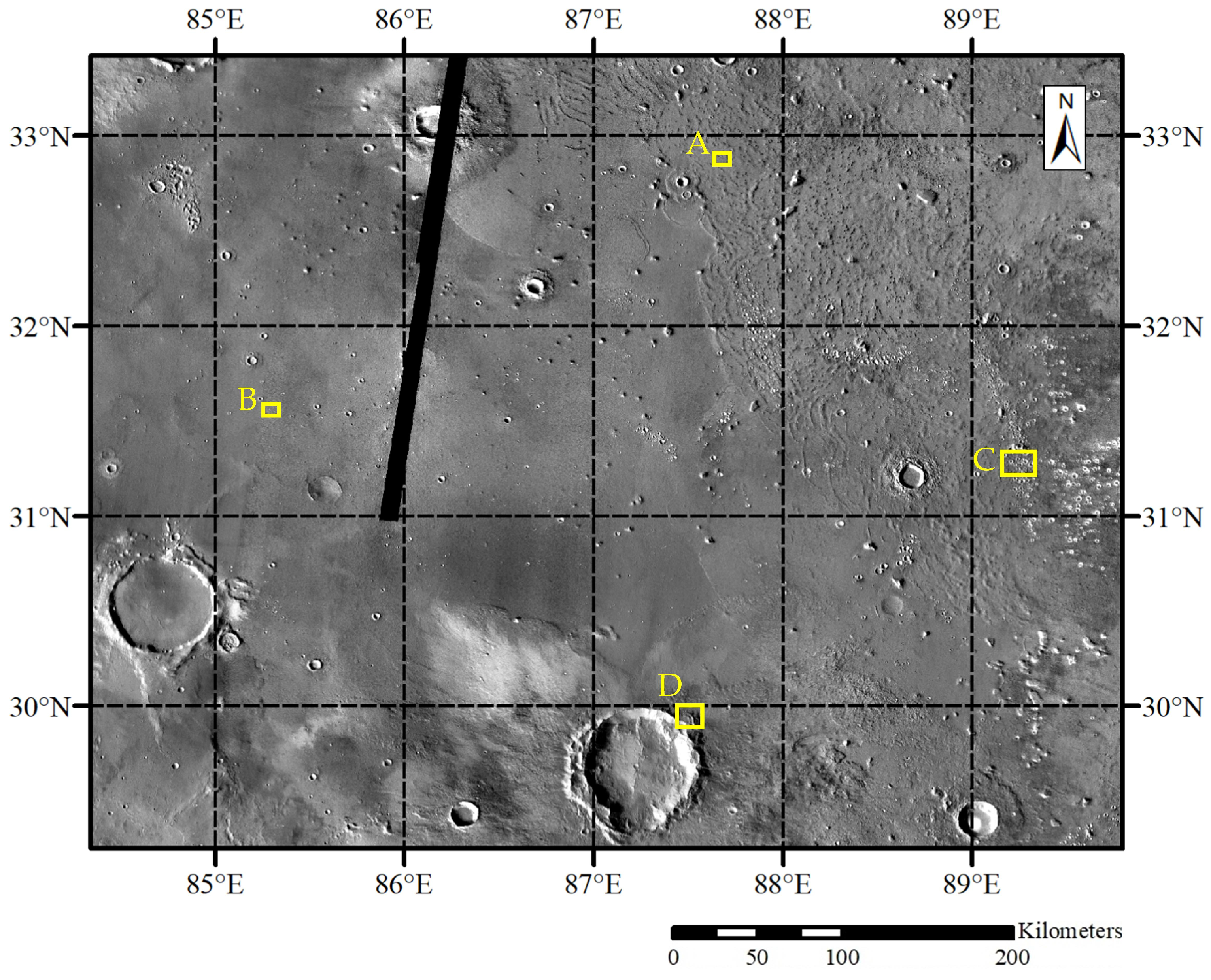
4.1. Study Area
4.2. Dataset
4.3. Comparisons
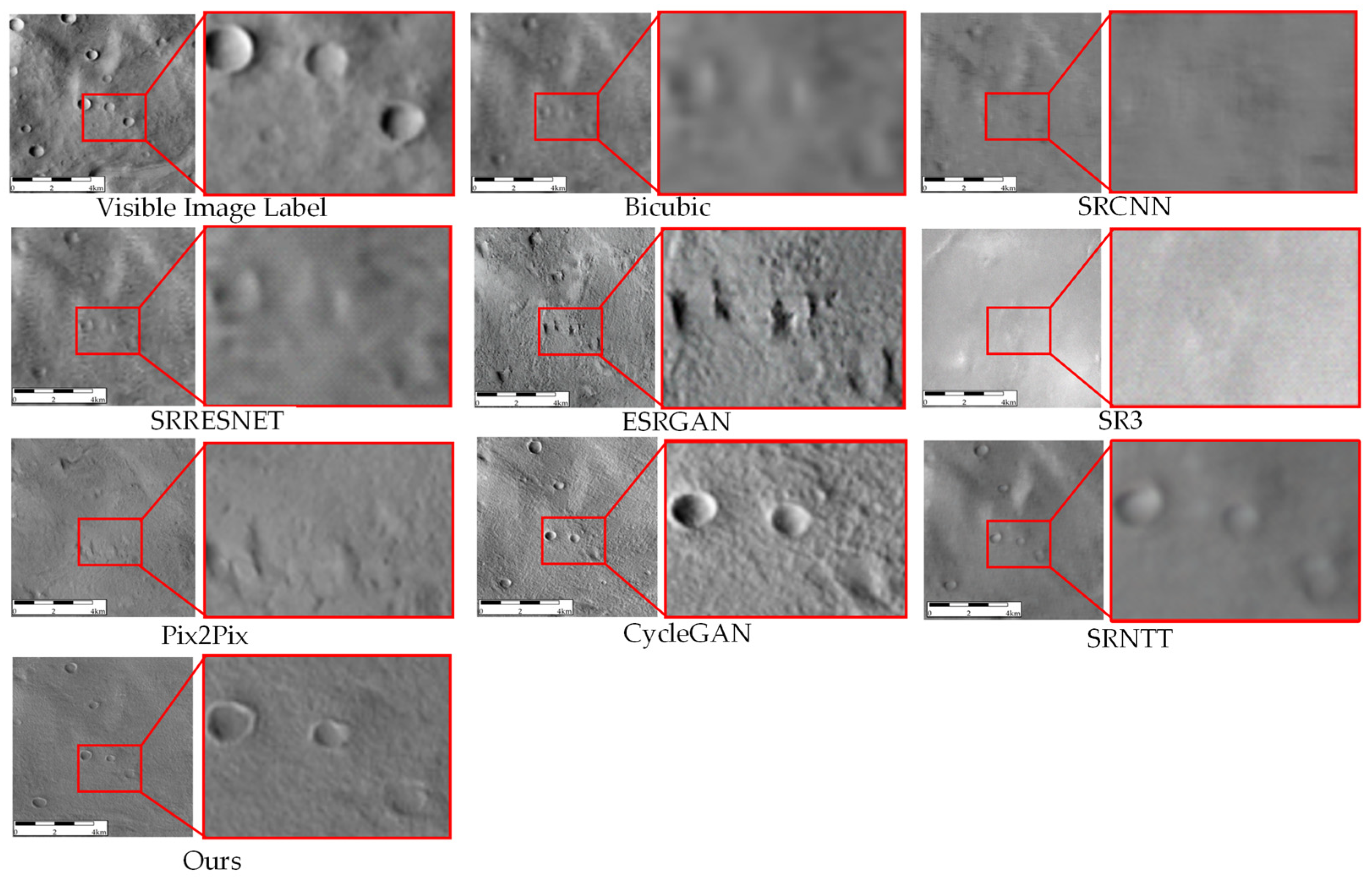
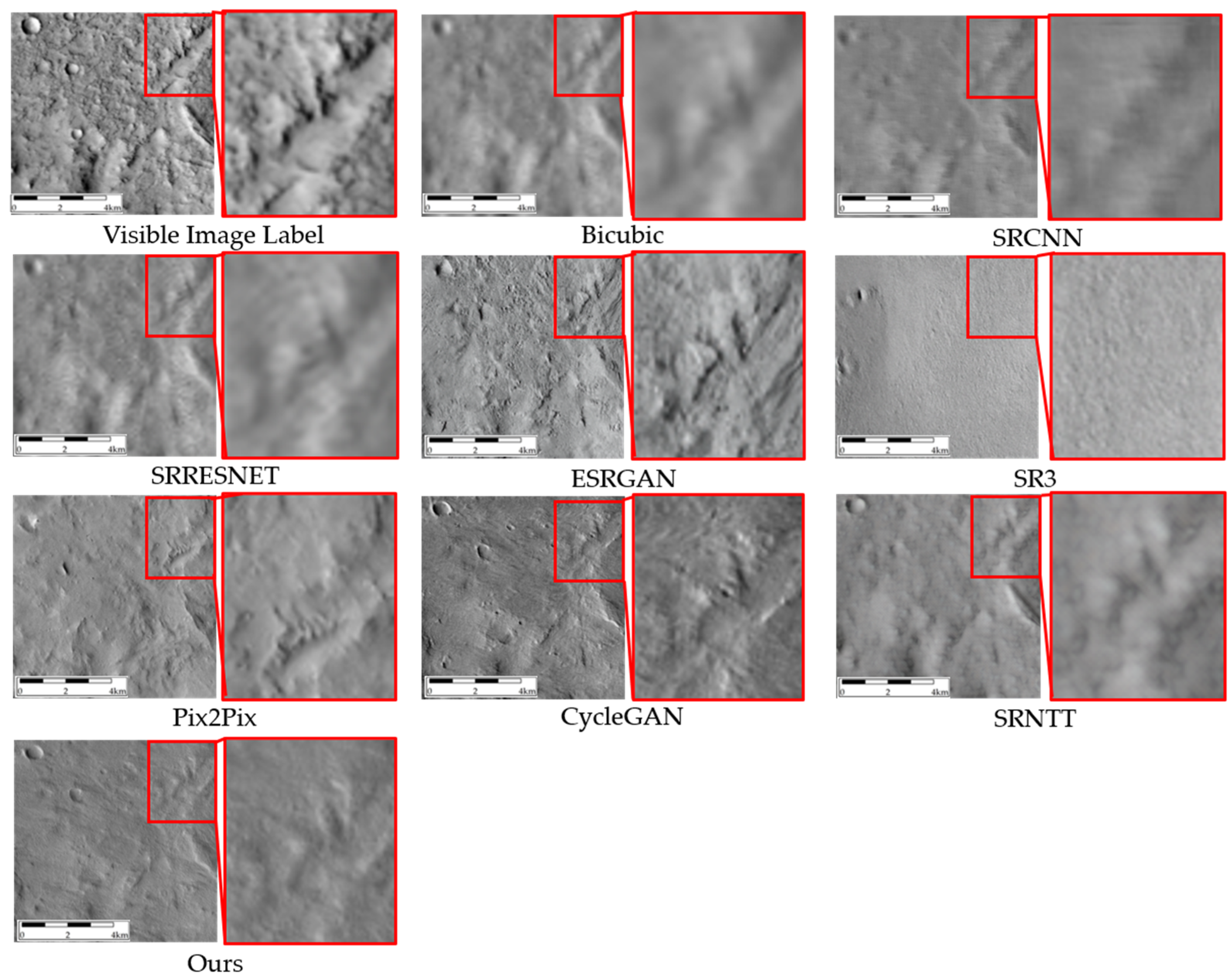
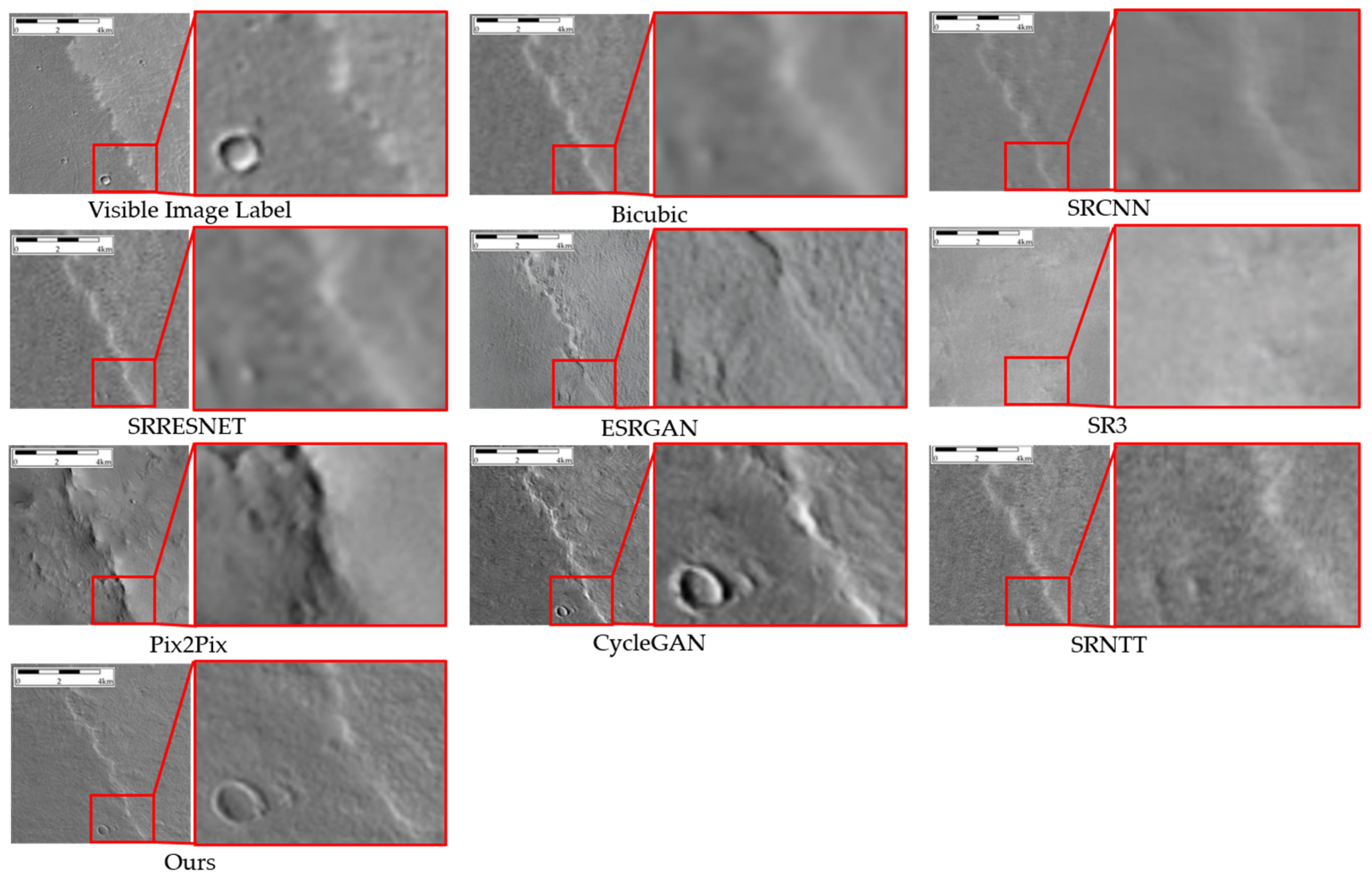
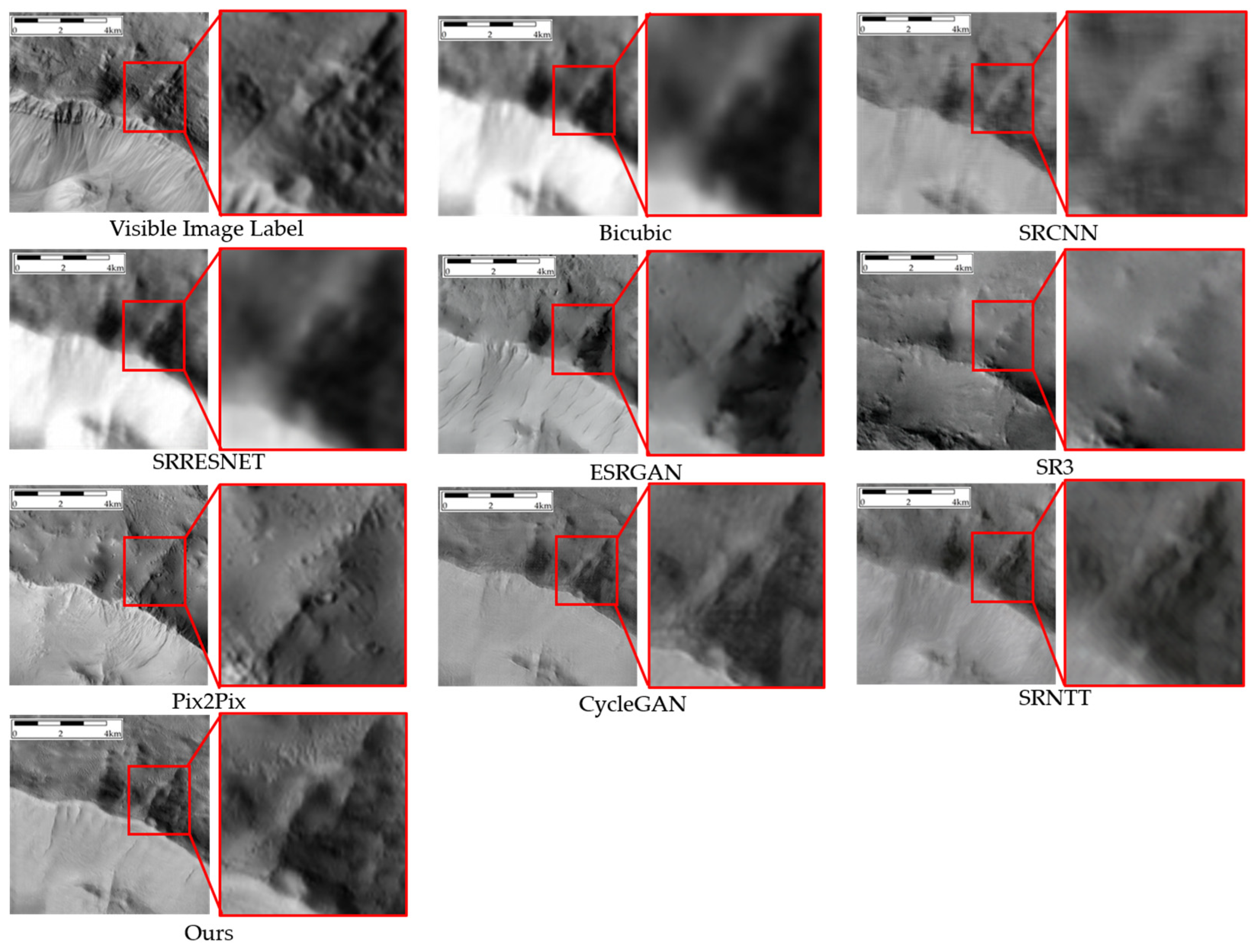
4.3.1. Comparison Between Proposed Thermal Infrared Image Super-Resolution Reconstruction Method and Comparing Methods
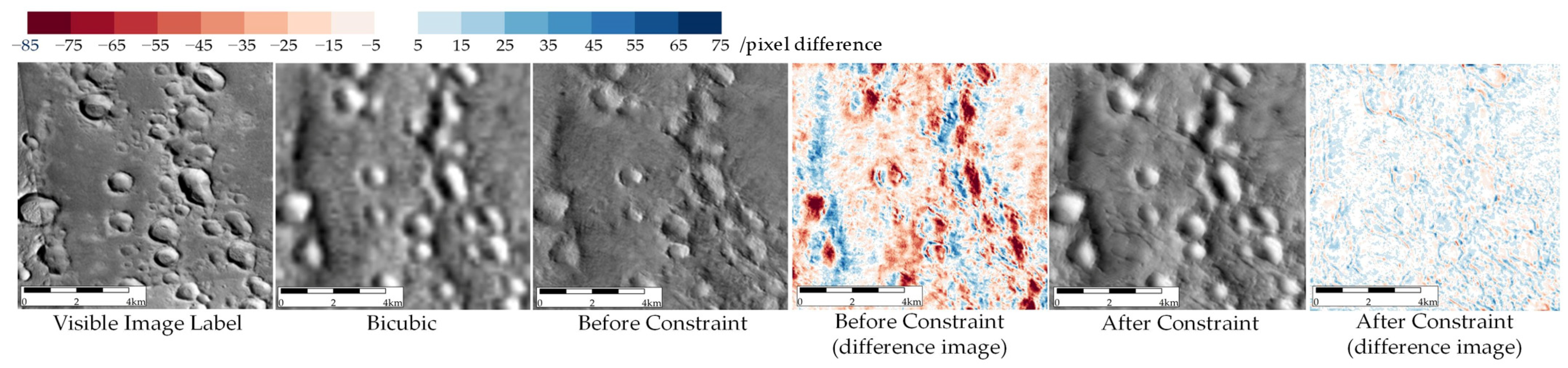
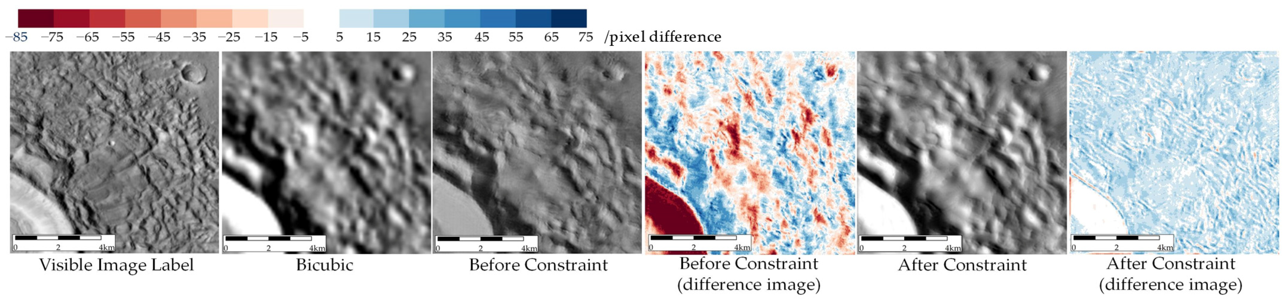
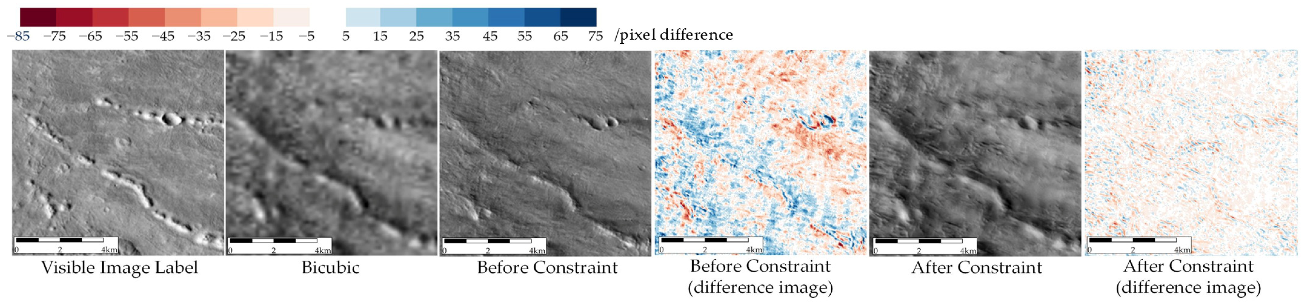
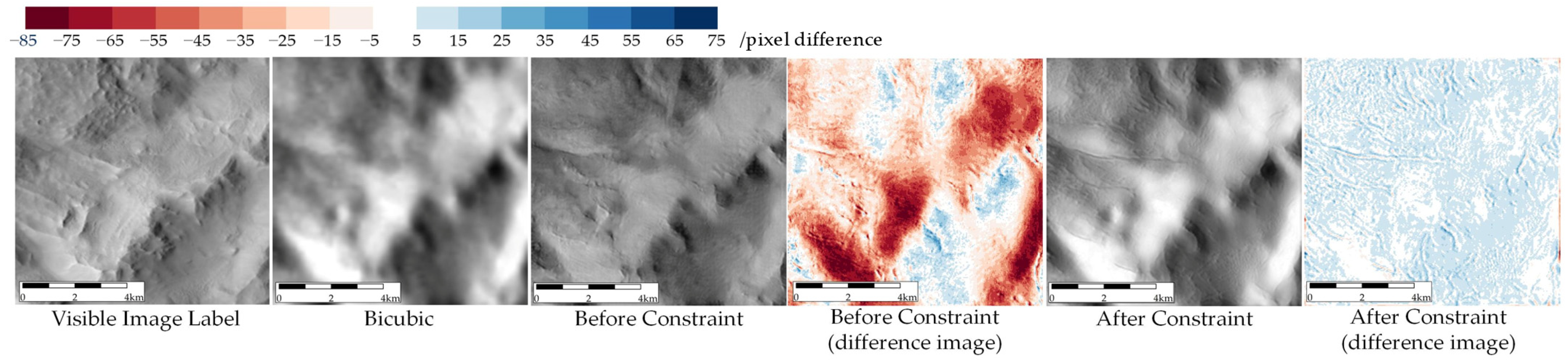
4.3.2. Comparison Before and After Thermal Radiation Flux Constraints
5. Results and Discussion
5.1. Discussion on Experimental Results of Thermal Infrared Image Super-Resolution Reconstrction
5.2. Discussion on Experimental Results of Thermal Radiation Flux Constraint
5.3. Application
6. Conclusions
- A super-resolution reconstruction method referenced by visible light image is proposed. Based on the principle of domain adaptation, a super-resolution network with a two-stage upsampling structure is designed, which utilizes visible light image textures as references. This network is trained on unpaired datasets with distinct domain characteristics, which employed to enable cross-domain representation alignment. Experimental results demonstrate that the proposed method significantly improves the visual quality of Mars thermal infrared imagery and maintains its correlation with the original imagery at the same time.
- A thermal radiation flux consistency constraint method is proposed. Based on the original low-resolution thermal infrared image, a Gradient-extraction network and an Intensity-extraction network are designed to separate the high-frequency boundary information and low-frequency background information in the original image. The consistency of the thermal radiation flux is then constrained by controlling the sum of pixel values between the resulting image and the original thermal infrared image within the same coverage. Experimental results demonstrate that this method can ensure the consistency of thermal radiation flux, making the resulting images more suitable for scientific research related to thermal radiation properties.
Author Contributions
Funding
Data Availability Statement
Conflicts of Interest
References
- Yu, D.; Sun, Z.; Meng, L.; Shi, D. Development History and Future Prospects of Mars Exploration. J. Deep Space Explor. 2016, 3, 108–113. (In Chinese) [Google Scholar] [CrossRef]
- Gou, S.; Yue, Z.; Di, K.; Zhang, X. Progress in the Detection of Hydrous Minerals on the Martian Surface. J. Remote Sens. 2017, 21, 531–548. (In Chinese) [Google Scholar] [CrossRef]
- Tao, Y.; Conway, S.J.; Muller, J.-P.; Putri, A.R.D.; Thomas, N.; Cremonese, G. Single Image Super-Resolution Restoration of TGO CaSSIS Colour Images: Demonstration with Perseverance Rover Landing Site and Mars Science Targets. Remote Sens. 2021, 13, 1777. [Google Scholar] [CrossRef]
- Li, C.; Zhang, R.; Yu, D.; Dong, G.; Liu, J.; Geng, Y.; Sun, Z.; Yan, W.; Ren, X.; Su, Y.; et al. China’s Mars Exploration Mission and Science Investigation. Space Sci. Rev. 2021, 217, 57–81. [Google Scholar] [CrossRef]
- Malin, M.C.; Bell, J.F.; Cantor, B.A.; Caplinger, M.A.; Calvin, W.M.; Clancy, R.T.; Edgett, K.S.; Edwards, L.; Haberle, R.M.; James, P.B.; et al. Context Camera Investigation on Board the Mars Reconnaissance Orbiter. J. Geophys. Res. 2007, 112, 1–25. [Google Scholar] [CrossRef]
- Wilhelm, T.; Geis, M.; Püttschneider, J.; Sievernich, T.; Weber, T.; Wohlfarth, K.; Wöhler, C. DoMars16k: A Diverse Dataset for Weakly Supervised Geomorphologic Analysis on Mars. Remote Sens. 2020, 12, 3981. [Google Scholar] [CrossRef]
- Christensen, P.R.; Jakosky, B.M.; Kieffer, H.H.; Malin, M.C.; McSween, H.Y., Jr.; Nealson, K.; Mehall, G.L.; Silverman, S.H.; Ferry, S.; Caplinger, M.; et al. The Thermal Emission Imaging System (Themis) for the Mars 2001 Odyssey Mission. In Mars Odyssey Mission; Springer: Dordrecht, The Netherlands, 2004; pp. 85–130. [Google Scholar] [CrossRef]
- Jakosky, B.M.; Lin, R.P.; Grebowsky, J.M.; Luhmann, J.G.; Beutelschies, G.; Priser, T.; Acuna, M.; Andersson, L.; Baird, D.; Baker, D.; et al. The Mars Atmosphere and Volatile Evolution (MAVEN) Mission. Space Sci. Rev. 2015, 195, 3–48. [Google Scholar] [CrossRef]
- Edwards, C.S.; Nowicki, K.J.; Christensen, P.R.; Hill, J.; Gorelick, N.; Murray, K. Mosaicking of Global Planetary Image Datasets: 1. Techniques and Data Processing for Thermal Emission Imaging System (THEMIS) Multi-Spectral Data. J. Geophys. Res. 2011, 116, 3755–3772. [Google Scholar] [CrossRef]
- Christensen, P.R.; Bandfield, J.L.; Hamilton, V.E.; Ruff, S.W.; Kieffer, H.H.; Titus, T.N.; Malin, M.C.; Morris, R.V.; Lane, M.D.; Clark, R.L.; et al. Mars Global Surveyor Thermal Emission Spectrometer Experiment: Investigation Description and Surface Science Results. J. Geophys. Res. Atmos. 2001, 106, 1370. [Google Scholar] [CrossRef]
- Christensen, P.R.; Bandfield, J.L.; Bell, J.F., III; Gorelick, N.; Hamilton, V.E.; Ivanov, A.; Jakosky, B.M.; Kieffer, H.H.; Lane, M.D.; Malin, M.C.; et al. Morphology and composition of the surface of Mars: Mars Odyssey THEMIS results. Science 2003, 300, 2056–2061. [Google Scholar] [CrossRef]
- Christensen, P.R. Formation of recent martian gullies through melting of extensive water-rich snow deposits. Nature 2003, 422, 45–48. [Google Scholar] [CrossRef] [PubMed]
- Sharma, R.; Srivastava, N. Detection and Classification of Potential Caves on the Flank of Elysium Mons, Mars. Res. Astron. Astrophys. 2022, 22, 10–21. [Google Scholar] [CrossRef]
- Hughes, C.G.; Ramsey, M.S. Super-resolution of THEMIS thermal infrared data: Compositional relationships of surface units below the 100 meter scale on Mars. Icarus 2010, 208, 704–720. [Google Scholar] [CrossRef]
- Wang, Q.; Ma, W.; Liu, S.; Tong, X.; Atkinson, P.M. Data Fidelity-Oriented Spatial-Spectral Fusion of CRISM and CTX Images. ISPRS J. Photogramm. Remote Sens. 2025, 220, 172–191. [Google Scholar] [CrossRef]
- Cheng, K.; Rong, L.; Jiang, S.; Zhan, Y. Overview of Remote Sensing Image Super-Resolution Reconstruction Technology Based on Deep Learning. J. Zhengzhou Univ. (Eng. Ed.) 2022, 43, 8–16. (In Chinese) [Google Scholar] [CrossRef]
- Chen, H.; He, X.; Qing, L.; Wu, Y.; Ren, C.; Sheriff, R.E.; Zhu, C. Real-World Single Image Super-Resolution: A Brief Review. Inf. Fusion 2022, 79, 124–145. [Google Scholar] [CrossRef]
- Liu, H.; Qian, Y.; Zhong, X.; Chen, L.; Yang, G. Research on super-resolution reconstruction of remote sensing images: A comprehensive review. Opt. Eng. 2021, 60, 100901. [Google Scholar] [CrossRef]
- Tao, H.; Tang, X.; Liu, J.; Tian, J.; Ungar, S.G.; Mao, S.; Yasuoka, Y. Superresolution Remote Sensing Image Processing Algorithm Based on Wavelet Transform and Interpolation. In Proceedings of SPIE, Hangzhou, China, 24–26 October 2002. [Google Scholar] [CrossRef]
- Kim, S.P.; Su, W.-Y. Recursive High-Resolution Reconstruction of Blurred Multiframe Images. IEEE Trans. Image Process. 1994, 2, 534–539. [Google Scholar] [CrossRef]
- Wang, W. Research on Infrared Super-Resolution Algorithms Based on Generative Adversarial Networks. Ph.D. Dissertation, University of Electronic Science and Technology of China, Chengdu, China, 2021. (In Chinese). [Google Scholar]
- Keys, R. Cubic Convolution Interpolation for Digital Image Processing. IEEE Trans. Acoust. Speech Signal Process. 1981, 29, 1153–1160. [Google Scholar] [CrossRef]
- Hou, H.; Andrews, H. Cubic Splines for Image Interpolation and Digital Filtering. IEEE Trans. Acoust. Speech Signal Process. 1978, 26, 508–517. [Google Scholar] [CrossRef]
- Zhang, X.; Wu, X. Image Interpolation by Adaptive 2-D Autoregressive Modeling and Soft-Decision Estimation. IEEE Trans. Image Process. 2008, 17, 887–896. [Google Scholar] [CrossRef] [PubMed]
- Teoh, K.K.; Ibrahim, H.; Bejo, S.K. Investigation on Several Basic Interpolation Methods for the Use in Remote Sensing Application. In Proceedings of the Conference on Innovative Technologies in Intelligent Systems and Industrial Applications, Cyberjaya, Malaysia, 12–13 July 2008; IEEE: Piscataway, NJ, USA, 2008; pp. 60–65. [Google Scholar] [CrossRef]
- Henry, S.; Peyma, O. High-Resolution Image Recovery from Image-Plane Arrays, Using Convex Projections. J. Opt. Soc. Am. A 1989, 6, 1715–1726. [Google Scholar] [CrossRef]
- Yang, X. Research on Frequency Domain and Spatial Domain Super-Resolution Reconstruction Technology of Remote Sensing Images. Ph.D. Dissertation, Harbin Institute of Technology, Harbin, China, 2024. (In Chinese). [Google Scholar]
- Patti, A.J.; Sezan, M.I.; Tekalp, A.M. Robust Methods for High-Quality Stills from Interlaced Video in the Presence of Dominant Motion. IEEE Trans. Circuits Syst. Video Technol. 1997, 7, 328–342. [Google Scholar] [CrossRef]
- Shang, L.; Liu, S.-F.; Sun, Z.-L. Image Super-Resolution Reconstruction Based on Sparse Representation and POCS Method. In Proceedings of the International Conference on Intelligent Computing, Fuzhou, China, 20–23 August 2015; Springer: Cham, Switzerland, 2015; pp. 348–356. [Google Scholar] [CrossRef]
- Dong, C.; Loy, C.C.; He, K.; Tang, X. Learning a Deep Convolutional Network for Image Super-Resolution. In Proceedings of the European Conference on Computer Vision (ECCV), Zurich, Switzerland, 6–12 September 2014; Springer: Cham, Switzerland, 2014; pp. 184–199. [Google Scholar] [CrossRef]
- Wang, Z.; Chen, J.; Hoi, S.C.H. Deep Learning for Image Super-Resolution: A Survey. IEEE Trans. Pattern Anal. Mach. Intell. 2021, 43, 3365–3387. [Google Scholar] [CrossRef] [PubMed]
- Anwar, S.; Khan, S.; Barnes, N. A Deep Journey into Super-Resolution: A Survey. ACM Comput. Surv. 2020, 53, 1–34. [Google Scholar] [CrossRef]
- Kim, J.; Lee, J.K.; Lee, K.M. Accurate Image Super-Resolution Using Very Deep Convolutional Networks. In Proceedings of the IEEE Conference on Computer Vision and Pattern Recognition (CVPR), Las Vegas, NV, USA, 27–30 June 2016; IEEE: Piscataway, NJ, USA, 2016; pp. 1646–1654. [Google Scholar]
- Lim, B.; Son, S.; Kim, H.; Nah, S.; Lee, K.M. Enhanced Deep Residual Networks for Single Image Super-Resolution. In Proceedings of the IEEE Conference on Computer Vision and Pattern Recognition Workshops (CVPRW), Honolulu, HI, USA, 21–26 July 2017; IEEE: Piscataway, NJ, USA, 2017; pp. 1132–1140. [Google Scholar] [CrossRef]
- Ahn, N.; Kang, B.; Sohn, K.-A. Fast, Accurate, and Lightweight Super-Resolution with Cascading Residual Network. In Proceedings of the European Conference on Computer Vision (ECCV), Munich, Germany, 8–14 September 2018; IEEE: Piscataway, NJ, USA, 2018. [Google Scholar]
- Tong, T.; Li, G.; Liu, X.; Gao, Q. Image Super-Resolution Using Dense Skip Connections. In Proceedings of the 2017 IEEE International Conference on Computer Vision (ICCV), Venice, Italy, 22–29 October 2017; IEEE: Piscataway, NJ, USA, 2017. [Google Scholar]
- Kim, J.; Lee, J.K.; Lee, K.M. Deeply Recursive Convolutional Network for Image Super-Resolution. In Proceedings of the Conference on Computer Vision and Pattern Recognition (CVPR), Las Vegas, NV, USA, 27–30 June 2016; IEEE: Piscataway, NJ, USA, 2016; pp. 4809–4817. [Google Scholar] [CrossRef]
- Zhang, Y.; Li, K.; Li, K.; Wang, L.; Zhong, B.; Fu, Y. Image Super-Resolution Using Very Deep Residual Channel Attention Networks. In Proceedings of the European Conference on Computer Vision (ECCV), Munich, Germany, 8–14 September 2018; Springer: Cham, Switzerland, 2018; pp. 294–310. [Google Scholar]
- Ledig, C.; Theis, L.; Huszár, F.; Caballero, J.; Cunningham, A.; Acosta, A.; Aitken, A.P.; Tejani, A.; Totz, J.; Wang, Z.; et al. Photo-Realistic Single Image Super-Resolution Using a Generative Adversarial Network. In Proceedings of the Conference on Computer Vision and Pattern Recognition Workshops (CVPRW), Honolulu, HI, USA, 21–26 July 2017; IEEE: Piscataway, NJ, USA, 2017; pp. 105–114. [Google Scholar] [CrossRef]
- Wang, X.; Yu, K.; Wu, S.; Gu, J.; Liu, Y.; Dong, C.; Qiao, Y.; Change Loy, C. ESRGAN: Enhanced Super-Resolution Generative Adversarial Networks. In Proceedings of the European Conference on Computer Vision (ECCV), Munich, Germany, 8–14 September 2018; Springer: Berlin/Heidelberg, Germany, 2018; pp. 63–79. [Google Scholar] [CrossRef]
- Li, J.; Zi, S.; Song, R.; Li, Y.; Hu, Y.; Du, Q. A Stepwise Domain Adaptive Segmentation Network with Covariate Shift Alleviation for Remote Sensing Imagery. IEEE Trans. Geosci. Remote Sens. 2022, 60, 5618515. [Google Scholar] [CrossRef]
- Yuan, Y.; Liu, S.; Zhang, J.; Zhang, Y.; Dong, C.; Lin, L. Unsupervised Image Super-Resolution Using Cycle-in-Cycle Generative Adversarial Networks. In Proceedings of the Conference on Computer Vision and Pattern Recognition Workshops (CVPRW), Salt Lake City, UT, USA, 18–22 June 2018; IEEE: Piscataway, NJ, USA, 2018; pp. 81401–81409. [Google Scholar] [CrossRef]
- McGill, G.E. Buried Topography of Utopia, Mars; Persistence of a Giant Impact Depression. Geophys. Res. Lett. 1989, 94, 2753–2759. [Google Scholar] [CrossRef]
- Séjourné, A.; Costard, F.; Gargani, J.; Soare, R.J.; Marmo, C. Evidence of an Eolian Ice-Rich and Stratified Permafrost in Utopia Planitia, Mars. Planet. Space Sci. 2012, 60, 248–254. [Google Scholar] [CrossRef]
- Wu, B.; Dong, J.; Wang, Y.; Li, Z.; Chen, Z.; Liu, W.C.; Zhu, J.; Chen, L.; Li, Y.; Rao, W. Characterization of the Candidate Landing Region for Tianwen-1—China’s First Mission to Mars. Earth Space Sci. 2021, 8, e2021EA001670. [Google Scholar] [CrossRef]
- Isola, P.; Zhu, J.-Y.; Zhou, T.; Efros, A.A. Image-to-Image Translation with Conditional Adversarial Networks. In Proceedings of the Conference on Computer Vision and Pattern Recognition Workshops (CVPRW), Honolulu, HI, USA, 21–26 July 2017; IEEE: Piscataway, NJ, USA, 2017; pp. 1125–1134. [Google Scholar] [CrossRef]
- Zhu, J.Y.; Park, T.; Isola, P.; Efros, A.A. Unpaired Image-to-Image Translation Using Cycle-Consistent Adversarial Networks. In Proceedings of the International Conference on Computer Vision (ICCV), Venice, Italy, 22–29 October 2017; IEEE: Piscataway, NJ, USA, 2017; pp. 2223–2232. [Google Scholar] [CrossRef]
- Saharia, C.; Ho, J.; Chan, W.; Salimans, T.; Fleet, D.J.; Norouzi, M. Image Super-Resolution via Iterative Refinement. IEEE Trans. Pattern Anal. Mach. Intell. 2023, 45, 4713–4726. [Google Scholar] [CrossRef]
- Zhang, Z.; Wang, Z.; Lin, Z.; Qi, H. Image super-resolution by neural texture transfer. In Proceedings of the IEEE/CVF Conference on Computer Vision and Pattern Recognition (CVPR), Long Beach, CA, USA, 15–20 June 2019; pp. 7982–7991. [Google Scholar] [CrossRef]


| Mission | Launch Time | Mission Goal | Sensors | Spatial Resolution |
|---|---|---|---|---|
| 2001 Mars Odyssey Mission | 2001.4 | Draw a global map depicting distribution of minerals on Mars | Thermal Emission Imaging System (THEMIS) | VIS: 18 m IR: 100 m |
| Mars Reconnaissance Orbiter | 2005.8 | Obtaining high-resolution images of the Martian surface. | Context Imager (CTX) | VIS: 5–6 m |
| Topographic Unit | Image Band | Image Size | Image Resolution | Channel | Image Number |
|---|---|---|---|---|---|
| Crater | VIS | 256 × 256 | 25 m | 1 | 4881 |
| IR | 64 × 64 | 100 m | 1 | 4881 | |
| Smooth Surface | VIS | 256 × 256 | 25 m | 1 | 5280 |
| IR | 64 × 64 | 100 m | 1 | 5280 | |
| Rough Surface | VIS | 256 × 256 | 25 m | 1 | 6942 |
| IR | 64 × 64 | 100 m | 1 | 6942 | |
| Ridge | VIS | 256 × 256 | 25 m | 1 | 8003 |
| IR | 64 × 64 | 100 m | 1 | 8003 |
| Category | Network | Parameter Counts | |
|---|---|---|---|
| Comparisons | spatial interpolation | Bicubic | - |
| CNN-based SISR | SRCNN | 57,281 | |
| SRRESNET | 1,536,384 | ||
| GAN-based SISR | ESRGAN | 16,697,987 (generator only) | |
| Pix2Pix | 54,407,809 (generator only) | ||
| CycleGAN | 11,365,633 (generator only) | ||
| Diffusion model-based SISR | SR3 | 27,436,547 (generator only) | |
| RefSR | SRNTT | 5,746,246 | |
| Ours | Ours | 11,365,633 (step1) + 49,868,971(step2) |
| Criterions | Equation | Parameters | Description | |
|---|---|---|---|---|
| Image Quality | Entropy (EN) | N is the gray scale of the image; is the probability of the gray scale; | Measures the complexity of the information in the image | |
| Spatial Frequency (SF) | RF is the row change rate; CF is the column change rate; H/W is the length and width of resulting image; is the value of pixel (i, j); | Measures the sharpness of the texture | ||
| Correlation with the Original Image | Peak Signal-to-Noise Ratio (PSNR) | X is the target image, is the resulting image; L is the maximum value of color contained in the image; | Calculates the ratio between the energy of the peak signal and the energy of the noise | |
| Structural Similarity Index Measure (SSIM) | X is the target image; is the resulting image; / are the mean and standard deviation of the image, is the covariance between X and ; C1/C2 are constant for result stability | Measures the similarity between two images. Average represents brightness, standard deviation represents contrast, correlation coefficient represents the structure similarity. | ||
| Image Fusion Quality Index of Wang And Bovik | a/b represent two images for fusion; ω is the sliding window; s represents the significance; is the local evaluation index between and ; represents the sum of the quality evaluations in the sliding window represents the significance of image a in the window ω | Measures the relative amount of edge information transferred from the original image to the resulting image; Evaluates the fusion quality based on sliding window. | ||
| EN_dist- (Output—vis) | SF_dist- (Output—vis) | SSIM+ | PSNR+ | + | |
|---|---|---|---|---|---|
| Bicubic | −0.0628 | −8.6128 | 0.4282 | 16.7767 | 0.1526 |
| SRCNN | 0.5942 | −5.8568 | 0.3488 | 15.7262 | 0.1584 |
| SRRESNET | 0.9095 | −3.5941 | 0.3150 | 15.3814 | 0.1708 |
| ESRGAN | 0.6023 | 2.5644 | 0.3504 | 15.3241 | 0.1679 |
| SR3 | 0.4175 | −3.5102 | 0.3347 | 15.2946 | 0.1559 |
| Pix2Pix | 0.1269 | −2.8519 | 0.3475 | 17.0112 | 0.1625 |
| CycleGAN | 0.3247 | −2.8792 | 0.2724 | 16.7694 | 0.1775 |
| SRNTT | 0.8408 | −5.5545 | 0.5935 | 16.6444 | 0.1722 |
| Ours | 0.0421 | −0.4089 | 0.3344 | 17.9100 | 0.1778 |
| MSE- | EN+ | SF+ | SSIM+ | PSNR+ | + | |
|---|---|---|---|---|---|---|
| Before Constraint | 0.0090 | 5.2781 | 9.7518 | 0.4547 | 18.7514 | 0.1868 |
| After Constraint | 0.0010 | 6.1784 | 12.7308 | 0.5444 | 20.6517 | 0.2021 |
Disclaimer/Publisher’s Note: The statements, opinions and data contained in all publications are solely those of the individual author(s) and contributor(s) and not of MDPI and/or the editor(s). MDPI and/or the editor(s) disclaim responsibility for any injury to people or property resulting from any ideas, methods, instructions or products referred to in the content. |
© 2025 by the authors. Licensee MDPI, Basel, Switzerland. This article is an open access article distributed under the terms and conditions of the Creative Commons Attribution (CC BY) license (https://creativecommons.org/licenses/by/4.0/).
Share and Cite
Lu, C.; Su, C. Super Resolution Reconstruction of Mars Thermal Infrared Remote Sensing Images Integrating Multi-Source Data. Remote Sens. 2025, 17, 2115. https://doi.org/10.3390/rs17132115
Lu C, Su C. Super Resolution Reconstruction of Mars Thermal Infrared Remote Sensing Images Integrating Multi-Source Data. Remote Sensing. 2025; 17(13):2115. https://doi.org/10.3390/rs17132115
Chicago/Turabian StyleLu, Chenyan, and Cheng Su. 2025. "Super Resolution Reconstruction of Mars Thermal Infrared Remote Sensing Images Integrating Multi-Source Data" Remote Sensing 17, no. 13: 2115. https://doi.org/10.3390/rs17132115
APA StyleLu, C., & Su, C. (2025). Super Resolution Reconstruction of Mars Thermal Infrared Remote Sensing Images Integrating Multi-Source Data. Remote Sensing, 17(13), 2115. https://doi.org/10.3390/rs17132115