Abstract
To effectively utilize the rich spectral information of hyperspectral remote sensing images (HRSIs), the fractional Fourier transform (FRFT) feature of HRSIs is proposed to reflect the time-domain and frequency-domain characteristics of a spectral pixel simultaneously, and an FRFT order selection criterion is also proposed based on maximizing separability. Firstly, FRFT is applied to the spectral pixels, and the amplitude spectrum is taken as the FRFT feature of HRSIs. The FRFT feature is mixed with the pixel spectral to form the presented spectral and fractional Fourier transform mixed feature (SF2MF), which contains time–frequency mixing information and spectral information of pixels. K-nearest neighbor, logistic regression, and random forest classifiers are used to verify the superiority of the proposed feature. A 1-dimensional convolutional neural network (1D-CNN) and a two-branch CNN network (Two-CNNSF2MF-Spa) are designed to extract the depth SF2MF feature and the SF2MF-spatial joint feature, respectively. Moreover, to compensate for the defect that CNN cannot effectively capture the long-range features of spectral pixels, a long short-term memory (LSTM) network is introduced to be combined with CNN to form a two-branch network C-CLSTMSF2MF for extracting deeper and more efficient fusion features. A 3D-CNNSF2MF model is designed, which firstly performs the principal component analysis on the spa-SF2MF cube containing spatial information and then feeds it into the 3-dimensional convolutional neural network 3D-CNNSF2MF to extract the SF2MF-spatial joint feature effectively. The experimental results of three real HRSIs show that the presented mixed feature SF2MF can effectively improve classification accuracy.
1. Introduction
Hyperspectral remote sensing images (HRSIs) are continuous, multi-band, high-resolution image data with rich and unique spectral features and spatial information [1,2]. HRSIs are widely used in various domains, especially agriculture, vegetation monitoring, and geological surveys [3,4,5].
HRSIs have rich spectral information, but with the increase in dimensionality, the spectral information is richer, the data amount also rises sharply, and complex mathematical calculations and model training are needed for classification, which makes it easier to appear the “Hughes” phenomenon [6]. Thus, dimensionality reduction operations are usually performed before HRSI classifications, such as principal components analysis (PCA) and linear discriminant analysis (LDA) [7,8,9]. After completing the dimensionality reduction operation to obtain the low-dimensional spatial data, some specific methods can be applied for clustering. For instance, Wang et al. [2] proposed a projection clustering approach for large-scale hyperspectral images. Their method simultaneously learns a pixel–anchor map and an anchor–anchor map in the projection space while introducing double stochastic constraints to optimize the anchor–anchor map, enabling efficient clustering of large-scale HRSI datasets. Beyond clustering, classification represents another crucial task in HRSI processing. HRSIs have rich spectral information, so networks such as deep belief networks (DBNs) and stacked auto-encoders (SAEs) have also been widely used for HRSI classifications [10,11]. However, both DBN and SAE can only process one-dimensional sequences, and convolutional neural networks (CNNs) can extract not only spectral features but also spatial features and thus gradually replace DBN and SAE as widely used deep learning models in HRSI classifications [12,13,14]. Hu designed a multilayer 1-dimensional CNN (1D-CNN) to classify the spectral pixel characteristics of HRSIs, and although it did not make use of the spatial information of HRSIs, its use of CNN to classify spectral pixels opened a new way of HRSI classifications, which greatly contributed to the development of HRSI classifications [15]. At the same time, because the same kind of features tend to show clustered distribution, there is a high possibility that features in neighboring areas are similar, and making full use of the spatial information of feature distribution is a major trend in the classification of HRSIs. Yue et al. used a 2-dimensional CNN (2D-CNN) to extract the spatial neighborhood features of HRSIs. They first applied PCA to HRSIs to reduce the dimensionality and eliminate the complex redundant information of the spectral and then extracted the spatial features of HRSI. The method did not fully use the spectral information of the pixels [16]. In addition, Yang proposed a two-channel deep CNN (Two-CNN), in which one branch used 1D-CNN to extract pixel spectral information, the other branch used 2D-CNN to extract neighborhood spatial information, and both spectral and spatial features were learned through two channels simultaneously [17].
CNNs are also often used in combination with other networks to compensate for the disadvantages that CNN cannot capture long-range features and the inadequacy of labeled samples. By introducing generative adversarial networks (GANs), a series of “deception-discrimination” game processes generate new samples that match the characteristics of a category with fewer labeled samples, which increases the number of labeled samples of that category for improving the classification accuracy [18]. Recurrent neural networks (RNNs) are adopted to capture the relationships of dependencies between the spectra in HRSIs, through which contextual information is extracted and combined with CNNs to improve classification accuracy [19]. Zhou proposed a two-branch spectral–spatial long- and short-term memory network, in which one branch extracted the long-time dependencies using a long short-term memory (LSTM) network for the spectral pixels, and the other branch first extracted the first principal component, expanded the pixel-centered neighborhood into a vector form, and then learned the spatial features of the central pixel one by one using LSTM to obtain the joint spectral–spatial results [20].
Three-dimensional CNNs (3D-CNNs) suit the three-dimensional structure of HRSIs and extract both spectral and neighborhood spatial information. Roy combined 3D-CNN with 2D-CNN to construct the hybrid spectral CNN (HybridSN) model, which reduced the number of parameters and model optimization time while greatly improving the classification accuracy [21]. Huang proposed Densely Connected Convolutional Network (DenseNet), which connects the feature maps of all previous layers to the current layer at each layer to enhance feature reuse [22]. The spectral–spatial feature tokenization transformer (SSFTT) model is a novel lightweight network consisting of only one 3D convolutional layer and one 2D convolutional layer. By integrating this module with an attention mechanism, this framework can fully leverage the spectral–spatial information of HRSIs and effectively improve the classification accuracy [23]. Deep learning methods have been pushing forward in the field of hyperspectral image processing, such as Wang et al.’s capsule attention network (CAN) [24]. By combining the attention mechanism with the activity vectors of the capsule network, CAN effectively improves the feature representation of hyperspectral images and enhances computational efficiency.
Due to the influence of observation technology, environmental conditions, vegetation growth stage, and other factors, the spectral curves of different features may appear similar, increasing the difficulty of classifying HRSIs [25]. Notably, in the fields of signal detection and radar waveform identification, fractional Fourier transform (FRFT) has been proven to be an effective tool to analyze signals from multiple angles by introducing the rotation angle parameter, which breaks through the limitation of the traditional Fourier transform of observing signals only in the time or frequency domain. In signal detection, the energy-focusing effect is shown in a specific fractional order prediction domain to verify the effectiveness of FRFT in detecting the signal at the receiver [26]. The FRFT has also been widely used in radar waveform recognition. FRFT can handle radar waveforms with similar recognition distributions and improve recognition accuracy by mapping the signals to fractional-order Fourier domains [27]. These applications show that the multi-angle analysis capability of FRFT can provide new perspectives for the feature extraction of complex signals, and the problem of highly similar spectral profiles in HRSIs is essentially a challenge of signal feature extraction and separation. Therefore, the introduction of FRFT into the field of hyperspectral image classification is expected to alleviate the classification confusion due to spectral similarity by observing the signal characteristics from multiple perspectives.
With a change in the observation angle, the difference in the spectral curves of different features may become more obvious, and the phenomenon can thus be improved. The FRFT is a special form of Fourier transform. When the signal makes a Fourier transform, the observation angle of the signal will convert from the time domain to the frequency domain; however, the FRFT, in contrast to the conventional Fourier transform, introduces a rotation angle parameter, i.e., the order, whose transform domain is neither in the time domain nor in the frequency domain but at an arbitrary angle between the two and is at a new perspective when observing the signal. In addition, the Fourier transform is a global transform, which obtains the overall spectrum of the signal after the transformation, so the time-domain information of the signal will be lost. However, FRFT can reflect not only the characteristics of the time domain but also the characteristics of the frequency domain [28,29].
In this paper, fractional Fourier transform is applied to HRSIs’ feature extraction; this has the following advantages:
- (1)
- The Fourier transform can convert the observation angle of spectral pixels to the frequency domain and reflect the differences among the spectral bands of spectral pixels by the spectra of the pixels. However, the fractional Fourier transform, as a special Fourier transform with variable order, can amplify the differences among different spectral pixels at a suitable observation angle by adjusting the order of the fractional Fourier transform.
- (2)
- The Fourier transform results in global frequency characteristics of spectral pixels, which will lose the time-domain information, while the FRFT is between the time domain and the frequency domain, which can reflect both the time-domain and frequency-domain characteristics of spectral pixels.
CNNs can represent local features well, but the global relationship of spectral bands is lost in the limit of convolutional kernel size. Therefore, in this paper, we introduce LSTM to be combined with CNN, which can solve the problem of long-time dependence, interpret the intrinsic connection of different spectral bands of the pixels, and improve the discriminability of the features.
In this paper, a new feature, i.e., the FRFT feature of the spectral pixels of HRSIs, is presented, and a criterion for selecting the order of fractional Fourier transform is also proposed based on maximizing discriminability. Firstly, the fractional Fourier transform is applied to the spectral pixels, and the amplitude spectrum is taken as the FRFT feature of HRSIs. The FRFT feature is combined with the original spectral pixels to form the presented spectral and fractional Fourier transform mixed feature (SF2MF), which contains time–frequency mixing information and spectral information of pixels.
Four network models were also designed based on CNN and LSTM for further deep feature extraction and classification. In addition to the base 1D-CNN, we have designed two 2-branch networks, C-CLSTMSF2MF and Two-CNNSF2MF-Spa, and a 3D-CNNSF2MF model. C-CLSTMSF2MF introduces LSTM to learn the long-time dependency between spectral bands to compensate for the defect that CNN can only capture local features within the receptive field; one branch of Two-CNNSF2MF-Spa learns the spectral-FRFT features, the other branch learns the spatial neighborhood features, and the resulting deep features of the two branches are fed jointly to a fully connected layer for classification. For reducing the computing complexity, the SF2MF features are processed by PCA for dimensionality reduction before input into the 3D-CNNSF2MF network, and the deep features are further extracted for classification to validate the effectiveness of the presented FRFT features.
Experiments were first conducted on four measured hyperspectral datasets using three traditional shallow classifiers—K-nearest neighbor (K-NN), logistic regression (LR), and random forest (RF)—followed by classification experiments on the four proposed networks—1D-CNN, C-CLSTMSF2MF, Two-CNNSF2MF-Spa, and 3D-CNNSF2MF—and the 3D-CNNSF2MF network was compared with existing HybridSN [21], DenseNet [22], and SSFTT [23] methods for comparison experiments. The experimental results show that the introduction of FRFT features can bring more discriminative information for classification, and the introduction of SF2MF into deep networks can further improve classification accuracy, especially when the percentage of training samples is small.
2. Spectral and Fractional Fourier Mixed Feature (SF2MF)
2.1. Fractional Fourier Transform
The FRFT can be defined from different perspectives. Currently, the commonly used definitions are those given by Ozaktas in terms of the integral transform and Namias in terms of the eigen-decomposition [30,31]. In this paper, the FRFT principle is described using the definition of the angle of integration given by Ozaktas.
In contrast to the fast Fourier transform (FFT), the FRFT introduces an angular rotation parameter, and the FRFT of a time-domain signal x(t) can be defined from the integration point of view as [32]
where the kernel function is
where δ(t) is the impulse function, , , n is an integer, is the angle of rotation of the time–frequency plane, and v is the order of the FRFT; we have
Equation (3) shows that for angles α that are not integer multiples of π, the computation of the FRFT of signal x(t) includes the following steps: multiply x(t) by a chirp, a Fourier transform, another multiplication by a chirp, and multiplication by a complex amplitude factor. It can be concluded that the inverse of an FRFT with the angle of α is the FRFT with the angle −α, that is,
We can see from Equation (4) that the FRFT of signal x(t) consists of the expression of x(t) on a set of basis functions , where u acts as a parameter to span the basis functions. The basis functions are orthonormal and are chirps, i.e., complex exponentials with linear frequency modulations [32]. Therefore, under certain order v, FRFT is a linear transformation that projects a signal to a functional space supported by . When v = 0, the functional space supported by represents the time domain, and v = 1 represents the frequency domain. When the order v of the FRFT gradually increases from 0 to 1, the result of the FRFT correspondingly transforms from the pure time-domain form of the signal to the pure frequency-domain form step by step. When the order v is a fraction between 0 and 1, the transformed signal is in the cross-plane of the time domain and the frequency domain, which is a mixed signal containing both time-domain and frequency-domain information, with the ability of joint time–frequency analysis.
Assuming that the spectral resolution of an HRSI is B, let denote an original spectral pixel. The FRFT of a pixel x can be expressed by [33]
where is the k-th fractional Fourier spectrum component of pixel x of order v and is the k-th Fourier spectrum component of x. Take the FRFT amplitude spectrum to obtain the fractional Fourier feature of pixel x. is the fractional spectrum of the original spectral pixel with angle α = vπ/2; it can be regarded as the expression of the spectral pixel on the set of basis chirps function . When the order v is in the fraction between 0 and 1, contains both time-domain and frequency-domain information, which is more beneficial for classification than a pure Fourier frequency spectrum. is concatenated with the spectral feature of pixel x to form the presented spectral and fractional Fourier mixture feature (SF2MF)
Direct feature splicing can obtain richer feature expression and is conducive to further deep feature extraction by CNN. SF2MF contains time–frequency mixing information and spectral information of pixels, thus having more interclass separability information than pure frequency and spectral features. In contrast to the spectral and frequency spectrum mixed feature (SFMF) [34], the SF2MF has a variable order, and the spectral curves are transformed differently with different orders of transformation so that the best viewing angle can be selected to distinguish the features. SF2MF contains the ability of time–frequency joint analysis, which Fourier transform does not have; it can better identify the category of pixels and improve the classification accuracy.
2.2. Optimal Order Selection for FRFT
Spectral information is an important feature of HRSI classification. However, two pixels of different classes may present the same spectral features. It can be solved by the shift of observation perspective, such as the Fourier transform, while the traditional Fourier transform will lose the local details of the time domain. As a special case of Fourier transform, FRFT can preserve the time-domain details while changing the viewing angle, and the smaller the order, the more details of the time domain are preserved. Therefore, it can be selected to retain appropriate time-domain details by changing the order to ensure that the resulting FRFT features contain both time-domain and frequency-domain features that comprise more separability information, which is a way to improve the classification accuracy.
Figure 1 shows the FRFT amplitude spectrums of different orders of a particular pixel of the Botswana dataset. The original spectral pixel curve is at v = 0, and the Fourier transform amplitude spectrum curve is at v = 1. It can be seen that the feature curve gradually changes from the original spectral pixel curve to the Fourier spectrum curve as the order increases. When the order v is small, the feature curve still retains the shape of the original spectral curve, which keeps fewer global features in the frequency domain while retaining more details in the time domain; when the order v is large, the FRFT amplitude spectrum curve tends to be in the shape of the Fourier amplitude spectrum curve, which enhances the global features while retaining fewer local details. When the FRFT order is 0 < v < 1, the proposed fractional Fourier feature has the joint time–frequency analysis capability to contain discriminative information for the phenomena of the same subject with different spectra and the different objects with the same spectrum simultaneously, which is effective for HSRI classification.
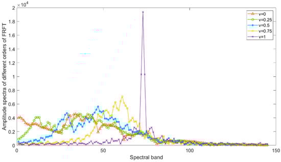
Figure 1.
Plots of FRFT of different orders.
An FRFT order selection criterion is presented based on maximizing separability. Assume that an HSRI dataset has a total of samples, , and C categories, the number of samples in the j-th category is ; then the intra-class scatter matrix is
and the interclass scattering matrix is
where denotes the v-order FRFT feature of the k-th sample in the j-th class of data, is the prior probability of class j, is the mean of the v-th order FRFT features of class j, and is the overall mean of the v-th order FRFT features, where , .The separability of the FRFT features is evaluated by
measures the distance between the mean of each category and the global mean. A larger indicates longer distances among different categories and better interclass separability. measures the degree of dispersion of the samples within classes, and a smaller means the samples within classes scatter more compactly, i.e., the samples of the same class are more similar. Thus, the separability of the data can be evaluated by J. Maximizing J can maximize the separability, leading to better classification results.
Thus, the optimal order v of the FRFT can be chosen by
In this paper, the order step in calculating the separability value of the FRFT of each order is 0.01, and the order v corresponding to the maximum separability value is selected. The selected FRFT order guarantees that the FRFT feature has a characteristic of more compactness within classes and more dispersion between classes and thus has better separability. Figure 2 shows the plot of separability value J varying with FRFT order v for four real HSRI datasets.
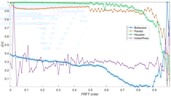
Figure 2.
Curves of separability value J varying with FRFT order v.
As can be seen in Figure 2, when FRFT order 0 < v < 1, the Botswana dataset has a very distinct peak near 1, the Indian Pines dataset has a distinct peak near 0, and the Houston and Pavia University datasets are more fluctuating but also have more distinct peaks, which further validates the validity of the selected FRFT orders. As the order changes, the separability value also changes, and the optimal order of each dataset is different due to the sample differences. In this paper, the order step is 0.01, and the optimal order for each dataset is selected according to the separability values of the FRFT features of different orders v. The optimal orders of the Botswana, Pavia University, Houston, and Indian Pines datasets are 0.98, 0.48, 0.09, and 0.02. The results of the MD classifier showed that the optimal classification results were in the vicinity of the selected order.
The Indian Pines dataset was obtained by imaging a patch of Indian Pines in Indiana, U.S.A. Most of the objects in the imaged area were crops, and the plants were in the growing season at the time, so the spectral curves of each object were very similar. Figure 3 shows the difference curves of the original means compared to the difference curves of the FRFT means of two objects having very similar original spectral curves. The difference curves of the means between classes 2 and 11 and those between classes 3 and 11 are shown in Figure 3, where class 2 is Corn-notill, class 3 is Corn-mintill, and class 11 is soybean-mintill. In Figure 3, 2&11-spe-MDC denotes the difference curves of the spectral means of classes 2 and 11, and 2&11-FRFT-MDC denotes the difference curves of the FRFT means of classes 2 and 11. The difference curves are normalized for better observation. Figure 3 shows that the FRFT difference curve has a larger mean and a more significant variance. The mean value of the difference curve represents the overall difference between two similar classes, and the larger the mean value, the more the difference between the two classes; the variance of the difference curve reflects the degree of fluctuation of the difference curve between the two classes, and the larger the variance, the more obvious the difference between the two classes, which is more conducive to classification. The mean and variance of the difference curves after the FRFT are larger, indicating that the overall differences in the characteristics of the two classes were greater after FRFT, which is beneficial for classification.
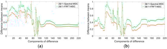
Figure 3.
Difference curves of Indian Pines dataset: (a) normalized difference curve between the mean values of Class 2 and Class 11; (b) normalized difference curve between the mean values of Class 3 and Class 11.
3. Network Models
To further extract deep features, this paper designs four network models for deep feature extraction and terrain classification, which verifies that introducing the proposed SF2MF feature into CNN can improve the classification accuracy. The four network models used are a 1-dimensional convolutional neural network (1D-CNN); two 2-branch CNN networks, C-CLSTMSF2MF and Two-CNNSF2MF-Spa; and a 3D-CNN after spectral PCA dimensionality reduction (3D-CNNSF2MF).
3.1. 1D-CNN
To obtain better classification performance, 1D-CNN is used to extract SF2MF depth features and perform classification. As shown in Figure 4, SF2MF is fed to the 1D-CNN for deep feature extraction and classification. When SF2MF is fed into 1D-CNN, the j-th feature map of the l-th layer after convolution is
where is the i-th feature map of layer , which is connected to the j-th feature map of layer l; ‘’ means convolution operation; is the convolution kernel corresponding to ; is the bias of the convolution kernel ; and represents the activation function.
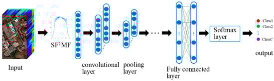
Figure 4.
Schematic diagram of 1D-CNN structure.
The 1D-CNN model contains multiple fully connected layers, where the last fully connected layer is used for classification. The feature vector learned by the l-th fully connected layer is
where is the feature vector of layer , is the weight matrix connecting layer l and layer , and is the bias vector of layer l.
Introducing SF2MF into CNN can extract SF2MF depth features and improve the classification accuracy.
3.2. C-CLSTMSF2MF
In hyperspectral data, the spectral energy of each band collectively forms the spectral features. However, 1D-CNNs have limited receptive fields, which leads to the loss of long-range dependency between bands when extracting spectral depth features. This deficiency may lead to suboptimal performance of 1D-CNNs in classification tasks utilizing spectral information. LSTM can achieve unique memory retention and forgetting functions through memory cells and gate structures, selectively preserving input information. When learning the t-th band, LSTM utilizes the information from the previous bands to update its internal state. Therefore, LSTM can utilize all spectral information and learn the relations between each spectral band and the bands ahead of it.
To compensate for the deficiency of limited local receptive fields in CNNs and to effectively extract long-range dependencies among spectral bands, a dual-branch network called C-CLSTMSF2MF is designed, which combines LSTM and CNN. C-CLSTMSF2MF extracts SF2MF-spectral fusion depth features through the fusion of two branches to provide richer feature expression and improve the classification performance.
Figure 5 shows the schematic diagram of the presented C-CLSTMSF2MF model. Two branches are 1D-CNN and CLSTM branches, which respectively take SF2MF and original spectral features as inputs.
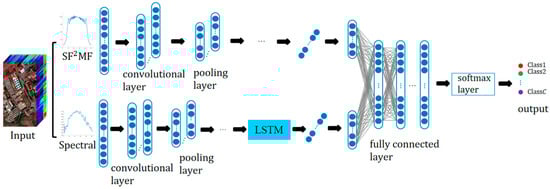
Figure 5.
Schematic diagram of C-CLSTMSF2MF structure.
In the 1D-CNN branch, the input SF2MF is for the n-th pixel. is the output after l convolutional and pooling operations, which is the SF2MF depth feature. The input of the CLSTM branch is the original spectral feature, and to compensate for the deficiency of CNN that can only extract local features, this branch combines CNN with LSTM to capture the inner correlation among spectral bands by using the memory-forgetting function of LSTM. The spectral feature of the n-th pixel input to this branch is , and is the output of after l convolution and pooling operations. Then, is fed into the LSTM to extract the long-distance relationship.
As shown in Figure 6, LSTM has three gate structures, called input gate, forget gate, and output gate, and its data processing and transmission process are completed by the three gate control structures. The computation process after the depth feature fed into the LSTM unit is
where represents the input data of the current LSTM unit, and , respectively, represent the cell state and hidden state at the t-th component. w and b represent the corresponding weights and biases, respectively; i, f, and o represent the input gate, forget gate, and output gate, respectively.
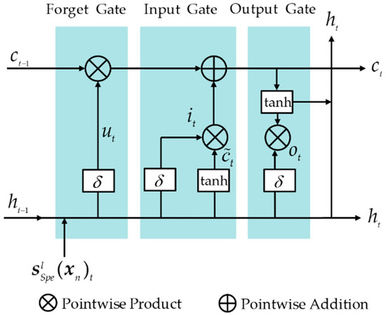
Figure 6.
Schematic structure of LSTM unit.
Figure 7 shows the schematic structure of LSTM. The input of the input gate is and the hidden state of the previous component is . The activation function causes the input gate to output a value between 0 and 1, controlling the selective retention of the new information . If the output is 0, no new information is retained at all. The input of the forget gate is , and the hidden state of the previous component is . If the output is 0, the cell state of the previous band is completely retained without any forgetting, and the current cell state is updated. The input of the output gate contains the current input , the hidden state of the previous component , and the current cell state . If the output value is 0, it means that no current information is output. The current hidden state is obtained by multiplying the output gate value with the current cell state and passing it through the tanh function.
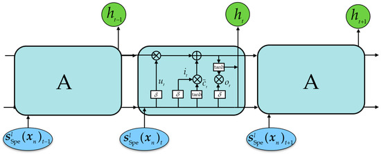
Figure 7.
Schematic structure of LSTM.
For spectral pixels, the receptive field of CNNs is constrained by their convolutional kernel size. This limitation leads to extracted features representing only localized spectral information within a finite neighborhood of each band while failing to capture global inter-band correlations across the entire spectral dimension. In contrast, LSTM can solve these limitations through the gating mechanism by dynamically learning the long-term dependencies of the spectral sequence through Equation (13), such that the final hidden state not only contains the local information of the current t-th band but also accumulates the global information from the previous (t − 1) bands into the cell state , thereby capturing the long-term dependencies of the entire spectral sequence . This mechanism enables LSTM to go beyond the local receptive field limitation of CNN and directly model the continuous trend of spectral curves and cross-band correlations.
On the other hand, if LSTM directly processes high-dimensional HRSI spectral pixels, it would encounter problems that include an excessive number of units, an oversized parameter quantity, and an overwhelming computational load. Therefore, the proposed CLSTM branch first employs CNN to perform deep feature extraction and dimensionality reduction on the original spectral pixels. The resulting low-dimensional deep spectral features containing neighborhood characteristics are fed into the LSTM, enabling further learning of deep features incorporating long-range dependencies.
The LSTM unit can retain and discard the hidden state of the previous component and the information of the current component through the cooperation of the three gate structures. By repeating the above process, the long-term dependencies among the components of can be learned. The sequence feature resulting from multiple convolution and pooling layers of CNN is fed into the LSTM network, and after memory-forget learning by B cascaded LSTM units, the output is obtained, where . Each component preserves the local deep independent characteristics of spectral bands through CNN. More importantly, it also captures long-range cross-band dependencies via the recursive transfer of LSTM’s hidden states. The LSTM model effectively mitigates the problems of gradient explosion and vanishing gradients, delivering robust and superior memory performance—this is the core advantage of LSTM.
To obtain the SF2MF–Spe depth feature, and are concatenated and sent to the fully connected layer. The output of the first fully connected layer can be expressed as
where W and b are the weight matrix and bias vector of the first fully connected layer, respectively. After several fully connected layers, a softmax regression layer completes the classification.
The input of the 1D-CNN branch is SF2MF. FRFT can perform a joint time–frequency analysis that contains time- and frequency-domain information. Thus, SF2MF is a feature with global information, so the deep features extracted by this branch contain global information. For the original spectral pixels, CNN can learn band context information by stacking convolutional layers to some extent. However, the ability to obtain long-distance information between bands is still limited. Therefore, the CLSTM branch utilizes LSTM to extract long-distance information between bands, but directly feeding high-dimensional spectral features into LSTM for deep feature extraction is very complex. Thus, in the CLSTM branch, the LSTM follows CNN, which can extract the depth features, reduce dimensionality, and improve computational efficiency. After multiple layers of CNN convolution and pooling, LSTM is employed for feature extraction. This approach leverages CNN’s ability to extract local features within the receptive field of the convolution kernel while utilizing LSTM to learn the long-range dependencies of deep spectral features, enabling comprehensive deep feature extraction of spectral pixels.
The presented two-branch network, C-CLSTMSF2MF, captures the long-distance band information with the help of LSTM to compensate for the global information that CNN lacks due to the limitations of receptive fields. Meanwhile, SF2MF depth features are concatenated with the depth spectral feature to extract SF2MF-spectral fusion depth features.
3.3. Two-CNNSF2MF-Spa
HRSIs belong to a special kind of image data and contain rich spectral and spatial information. Spectral information and spatial information correspond to the physical properties and distribution characteristics of the corresponding objects, respectively. These two types of information complement each other and constitute a comprehensive and accurate depiction of objects. The individual spectral or spatial information alone cannot accurately characterize the objects. To fully utilize the spatial information of HRSIs, a dual-branch network called Two-CNNSF2MF-Spa is designed based on 1D-CNN and 2D-CNN.
The structure of the presented Two-CNNSF2MF-Spa is shown in Figure 8. One branch is a 1D-CNN structure with the input SF2MF. The SF2MF of the n-th pixel is . is the output after l convolution and pooling operations, which can be regarded as the deep features of SF2MF. Another branch is the 2D-CNN structure, where the input is the spatial features of HRSIs. Therefore, the convolutional and pooling layers in this branch are all two-dimensional operations.
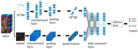
Figure 8.
Schematic diagram of Two-CNNSF2MF-Spa structure.
The experiment fuses information from all spectral bands and reduces noise by averaging the spectral bands of HRSIs. Then, cutting the adjacent pixels of the n-th pixel obtains the spatial pixel block of size as the input for the spatial branch.
The two branches obtain SF2MF depth feature and spatial depth feature after l convolution and pooling operations, respectively. To fully utilize the SF2MF depth feature and the spatial depth feature, and are directly concatenated, and the concatenated feature has a richer representation. To obtain the SF2MF-Spa fusion depth feature, is fed into the fully connected layer, and the output after the first fully connected layer is
After several fully connected layers, a softmax regression layer completes the classification.
The presented dual-branch network, Two-CNNSF2MF-Spa, can extract the SF2MF-Spa depth feature, which provides more accurate and sufficient ground object expression information and improves classification accuracy.
3.4. 3D-CNNSF2MF
HRSIs are three-dimensional images that not only cover the continuous spectral information of the target object but also contain its spatial information. Although Two-CNNSF2MF-Spa utilizes SF2MF information and spatial information, 3D-CNN can simultaneously apply convolutional operations to hyperspectral image data from three dimensions, extracting SF2MF and spatial depth features and improving the classification accuracy effectively.
The structure of the proposed 3D-CNNSF2MF is shown in Figure 9. To reduce the redundant information between bands and enhance the computational speed, the SF2MF cube that contains the spatial information is performed PCA first along the SF2MF dimension. The image after PCA contains most of the information of the original image. The pixel cube (h, q, and d are the height, width, and depth of the cube, respectively) composed of the n-th pixel and adjacent pixels is taken as the input to the 3D-CNN.
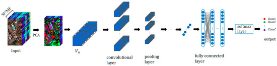
Figure 9.
Schematic diagram of 3D-CNNSF2MF structure.
The 3D-CNNSF2MF model can extract deep SF2MF and spatial features by utilizing 3D convolution operations on SF2MF and spatial dimensions. The convolution operation of 3D-CNNSF2MF is
where is the neuron at position of the j-th feature map of layer i; k is the number of channels connected to each other in the front and back layers; Hi and Qi represent the height and width of the convolution kernel, respectively; and Di is the scale size of the convolution kernel in the SF2MF dimension. is the weight of the convolution kernel for the k-th channel of the j-th feature map in layer i at position (h, q, d), and b is the bias of the j-th feature map on the neuron in layer i.
For the n-th pixel, is the SF2MF-spatial joint feature extracted after l layers of convolution and pooling operations. The output of the first fully connected layer obtained by feeding it to the fully connected layers for deep feature extraction is
where is the deeper SF2MF-spatial joint feature obtained, and after several fully connected layers, the probability of each category can be predicted through the softmax layer, thus completing the classification.
The 3D-CNNSF2MF model can obtain the SF2MF-space depth joint features through 3D convolution operation. This capability of deep joint feature extraction makes it possible to obtain richer and more accurate object description information compared to Two-CNNSF2MF-Spa, which can effectively improve classification accuracy.
4. Experimental Results
The optimal FRFT order v is selected for each HSRI using the divisibility value J. The orders selected for the Botswana, Pavia University, Houston, and Indian Pines datasets are 0.98, 0.48, 0.04, and 0.02, respectively. Three traditional shallow classifiers and four network models are adopted in this paper to validate the effectiveness of SF2MF.
4.1. Experimental Datasets
Four real hyperspectral datasets were used for the experiments in this paper, namely Botswana, Pavia University (PaviaU), Houston, and Indian Pines, shown in Figure 10, Figure 11, Figure 12 and Figure 13.
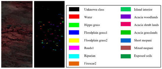
Figure 10.
False color image and ground truth of Botswana dataset.
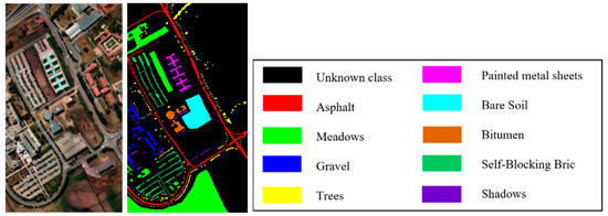
Figure 11.
False color image and ground truth of Pavia University dataset.
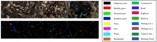
Figure 12.
False color image and ground truth of Houston dataset.
Figure 13.
False color image and ground truth of Indian Pines dataset.
The Botswana dataset imaging the Botswana area has a total of 242 bands, with 145 bands used in the experiment, excluding uncalibrated and noisy bands covering water absorption features. The image size is , with 14 classes and 3248 terrain pixels, excluding background pixels.
The Pavia University dataset imaging the University of Pavia, Italy, contains nine classes. Excluding the bands affected by noise, 103 bands were used in the experiment. The image has a size of 610 340 and contains 42,776 terrain pixels, excluding background pixels.
The Houston dataset, obtained by the ITRES CASI-1500 sensor, has a size of 349 1905, containing 144 bands. In addition to background pixels, it has 15,029 terrain pixels belonging to 15 terrain classes.
The Indian Pines dataset has 16 terrain classes with 220 spectral bands. The image size is 145 145, of which 10,249 pixels are terrain pixels.
4.2. Network Structure and Parameter Settings
Table 1 shows the CNN architecture for each of the four real datasets, i.e., Botswana, Pavia University, Houston, and Indian Pines, in this paper. I, C, S, F, and O represent the input, convolutional, pooling, fully connected, and output layers, respectively. For example, C2 is the convolutional layer, the second layer in the entire neural network. The learning rate is a key hyperparameter that controls the step size of the model parameter update. In this paper, the Adam optimizer is employed to dynamically adjust the parameter update direction using its adaptive learning rate property. Through experimental verification, the initial learning rate is set to 0.005. The batch size directly affects the stability of gradient update and memory occupation. Multiple experiments show that when the batch size is 10, the model can efficiently utilize GPU memory while ensuring gradient stability. All experiments are run independently 10 times, and the mean and standard deviation of the results are taken as the final evaluation index.

Table 1.
CNN parameter settings for four datasets.
Table 2 shows the CNN feature map size for each dataset.
Table 2.
CNN feature map size for four datasets.
4.3. Classification Results of Traditional Shallow Classifiers
In this paper, the K-NN, LR, and RF classifiers are adopted to complete the classification comparison experiments of Spe, SFMF, and SF2MF features. In this case, 20% of the data samples were randomly selected as training data, and the rest were testing data. The average overall accuracy (AOA) and the standard deviation (SD) are the results of ten runs. The classification results are shown in Table 3, where the optimal classification results for each classifier have been bolded, and K = 5 for the K-NN classifier.
Table 3.
Classification results of Botswana dataset on shallow classifiers.
As can be seen from Table 3, with 20% training samples in Botswana dataset, compared to the original spectral features Spe, the presented SF2MF improved the AOAs on K-NN, LR, and RF classifiers by 3.10%, 0.48%, and 1.36%, respectively; compared to SFMF, SF2MF improved the AOAs on K-NN, LR, and RF classifiers by 0.89%, 0.40%, and 0.19%, respectively. The classification accuracy of the proposed SF2MF is higher compared to the other two features, indicating that SF2MF has more accurate terrain description information that improves the classification accuracy of the Botswana dataset.
As can be seen from Table 4, with 20% of the training samples, compared to the original spectral feature Spe, SF2MF improved the AOAs on the K-NN, LR, and RF classifiers by 1.62%, 3.79%, and 1.55%, respectively. Compared to SFMF, SF2MF improved the AOAs on the K-NN, LR, and RF classifiers by 0.95%, 1.11%, and 0.33%, respectively. Compared to the other two features, the classification accuracy improvement of SF2MF is very significant, which verifies the effectiveness of SF2MF.
Table 4.
Classification results of PaviaU dataset on shallow classifiers.
As can be seen from Table 5, with 20% of the training samples in the Houston dataset, compared to the original spectral feature Spe, SF2MF improves the AOAs on the K-NN, LR, and RF classifiers by 3.13%, 7.28%, and 2.23%, respectively. SF2MF improved the AOAs on the K-NN, LR, and RF classifiers by 0.42%, 1.12%, and 0.50%, respectively, compared to SFMF. The proposed SF2MF feature improved the classification accuracy, indicating that the presented SF2MF has richer divisibility information and more accurate information on terrain representation than Spe and SFMF, which can effectively improve the classification accuracy.
Table 5.
Classification results of Houston dataset on shallow classifiers.
As can be seen from Table 6, with 20% training samples, compared to the original spectral feature Spe, SF2MF improved the AOAs on the K-NN, LR, and RF classifiers by 2.59%, 3.29%, and 1.33%, respectively. The AOAs of SF2MF are 2.59%, 2.29%, and 2.04% higher than those of SFMF on the K-NN, LR, and RF classifiers, respectively.
Table 6.
Classification results of Indian Pines dataset on shallow classifiers.
From Table 3, Table 4, Table 5 and Table 6, it can be seen that, compared to the original spectral feature Spe and SFMF, the proposed SF2MF has a better classification effect on the shallow classifiers, which indicates that SF2MF has more abundant information on terrain discriminability and superior terrain characterization capability, which can more accurately represent and discriminate the terrains to enhance the classification performance.
4.4. Classification Results of Networks
To verify the effectiveness of the proposed features, four HSRIs, i.e., Botswana, Pavia University, Houston, and Indian Pines, were adopted in the experiments, and 5%, 10%, and 20% of each class’s data were randomly selected as training data, and the remaining data were testing data. Classification experiments were conducted using the proposed networks, 1D-CNN, C-CLSTMSF2MF, Two-CNNSF2MF-Spa, and 3D-CNNSF2MF, and comparison experiments were conducted between 3D-CNNSF2MF and the existing HybridSN, DenseNet, and SSFTT methods. The AOA, Kappa coefficient, and SD were used as evaluation metrics under the same experimental conditions, and the optimal recognition of each column is bolded in Table 7, Table 8, Table 9, Table 10, Table 11, Table 12 and Table 13.
Table 7.
Classification results of Botswana dataset.
Table 8.
Classification results of the Pavia University dataset.
Table 9.
Classification results of the Houston dataset.
Table 10.
Classification results of the Indian Pines dataset.
Table 11.
Classification results of 5% training samples of Botswana, Pavia University, Houston, and Indian Pines datasets.
Table 12.
Classification results of 10% training samples of Botswana, Pavia University, Houston, and Indian Pines datasets.
Table 13.
Classification results of 20% training samples of Botswana, Pavia University, Houston, and Indian Pines datasets.
Table 7 shows the classification results of the Botswana dataset for the proposed features SF2MF with Spe and SFMF on the four network models for 5%, 10%, and 20% of the training samples, respectively. From Table 7, it can be seen that SF2MF has superior classification accuracy on all four networks compared to Spe and SFMF. Especially when the training samples are relatively small, the proposed features show a significant improvement in classification accuracy. In the case of small samples, the network only uses a limited number of samples for training, resulting in limited expression ability of the deep features captured by the network. While SF2MF introduces FRFT features with the ability of the joint analysis of time–frequency information, the expression of terrain characteristics is more abundant and comprehensive, which can effectively improve the classification accuracy. In addition, the SD values of SF2MF are smaller than those of other features, which suggests that SF2MF is more stable in classification tasks.
Figure 14 shows the classification results of the Botswana dataset for the proposed feature SF2MF with Spe and SFMF on the four network models when using 5% training samples. It is evident that SF2MF can provide a superior feature representation for classification compared to Spe and SFMF.
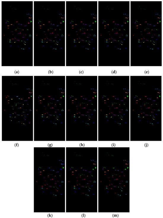
Figure 14.
Botswana dataset classification map: (a) ground truth; (b) spectral feature in 1D-CNN; (c) SFMF in 1D-CNN; (d) SF2MF in 1D-CNN; (e) spectral feature in C-CLSTM; (f) SFMF in C-CLSTM; (g) SF2MF in C-CLSTM; (h) spectral feature in Two-CNN; (i) SFMF in TWO-CNN; (j) SF2MF in Two-CNN; (k) spectral feature in 3D-CNN; (l) SFMF in 3D-CNN; and (m) SF2MF in 3D-CNN.
Table 8 lists the classification results of the Pavia University dataset for SF2MF compared to Spe and SFMF on the four network models using 5%, 10%, and 20% training samples, respectively. Table 8 shows that the proposed feature SF2MF has the optimal AOA and Kappa values in all four network models. In addition, SF2MF has smaller SD values, indicating superior stability of SF2MF and validating its effectiveness in terrain classification. Meanwhile, compared to the other two features, SF2MF has a superior classification effect in the case of small samples.
Table 9 shows the classification results of the Houston dataset for the proposed SF2MF compared to Spe and SFMF on the four network models for 5%, 10%, and 20% of the training samples, respectively. Table 9 shows that SF2MF has the best AOA and Kappa values among all four network models, especially when the size of the training samples is relatively small, SF2MF has a significant improvement in classification accuracy. Moreover, the SD value of SF2MF is smaller than other features and more stable in the classification task, which indicates that the SF2MF method is more stable and can provide more separability information for classification, which validates the effectiveness of SF2MF.
Figure 15 shows the classification results of the Pavia University dataset for the proposed feature SF2MF compared to Spe and SFMF on the four network models when using 5% training samples. It is evident that SF2MF can provide a superior feature representation for classification compared to Spe and SFMF.
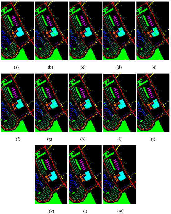
Figure 15.
Pavia University dataset classification map: (a) ground truth; (b) spectral feature in 1D-CNN; (c) SFMF in 1D-CNN; (d) SF2MF in 1D-CNN; (e) spectral feature in C-CLSTM; (f) SFMF in C-CLSTM; (g) SF2MF in C-CLSTM; (h) spectral feature in TWO-CNN; (i) SFMF in Two-CNN; (j) SF2MF in Two-CNN; (k) spectral feature in 3D-CNN; (l) SFMF in 3D-CNN; and (m) SF2MF in 3D-CNN.
Figure 16 shows the classification results of the Houston dataset for the proposed feature SF2MF compared to Spe and SFMF on the four network models when using 5% training samples. It is evident that SF2MF can provide a superior feature representation for feature classification compared to Spe and SFMF.
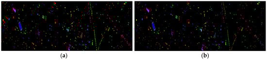
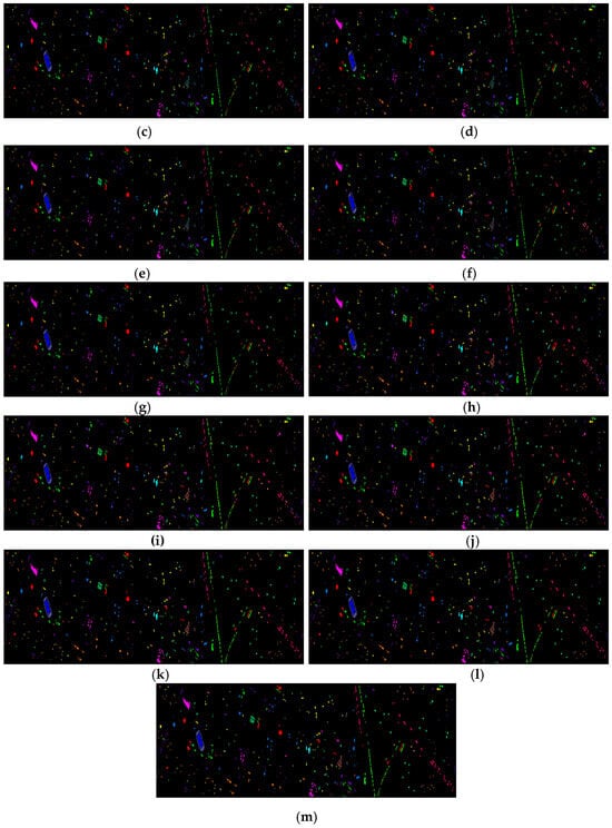
Figure 16.
Houston dataset classification map: (a) ground truth; (b) spectral feature in 1D-CNN; (c) SFMF in 1D-CNN; (d) SF2MF in 1D-CNN; (e) spectral feature in C-CLSTM; (f) SFMF in C-CLSTM; (g) SF2MF in C-CLSTM; (h) spectral feature in Two-CNN; (i) SFMF in Two-CNN; (j) SF2MF in TWO-CNN; (k) spectral feature in 3D-CNN; (l) SFMF in 3D-CNN; and (m) SF2MF in 3D-CNN.
Table 10 shows the results of Spe, SFMF, and SF2MF on the Indian Pines dataset using 5%, 10%, and 20% of the training samples on the four network models. Compared with Spe and SFMF, SF2MF has optimal AOA and Kappa values in all four network models, which is more beneficial for classification. The classification accuracy is significantly improved by SF2MF, especially under small-size training samples. The SF2MF method corresponds to a smaller SD value, which indicates that SF2MF has better stability and can provide more separable information for classification, verifying its effectiveness in feature classification.
Figure 17 shows the classification results of the Indian Pines dataset for the proposed feature SF2MF compared to Spe and SFMF on the four network models when using 10% training samples. Compared to the Spe and SFMF, SF2MF achieves higher classification accuracy among the four network models. Notably, SF2MF significantly improves the AOA and Kappa values with a small training sample size, suggesting that integrating FRFT can enrich the classification description. In the case of small samples, the deep features learned from limited training data are not sufficient to achieve accurate feature representations. The hybrid features of SF2MF provide richer terrain information, which helps the network learn to capture the deep features of the terrain features more accurately.
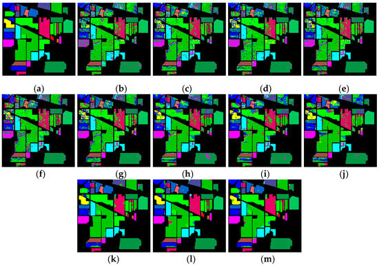
Figure 17.
Indian Pines dataset classification map: (a) ground truth; (b) spectral feature in 1D-CNN; (c) SFMF in 1D-CNN; (d) SF2MF in 1D-CNN; (e) spectral feature in C-CLSTM; (f) SFMF in C-CLSTM; (g) SF2MF in C-CLSTM; (h) spectral feature in TWO-CNN; (i) SFMF in TWO-CNN; (j) SF2MF in TWO-CNN; (k) spectral feature in 3D-CNN; (l) SFMF in 3D-CNN; (m) SF2MF in 3D-CNN.
To verify the effectiveness of the proposed hybrid features on different network models, we use HybridSN, DenseNet, and SSFTT models to complete the relevant comparison experiments. The AOA, average Kappa coefficient (AK), and SD of the ten runs are used to evaluate the effectiveness of the proposed features and the classification reliability. Table 11, Table 12 and Table 13 show the experimental results for each dataset at 5%, 10%, and 20% of the training samples, respectively, and the optimal recognition results are bolded.
As can be seen from Table 11, Table 12 and Table 13, the AOA of the SF2MF feature for the Botswana dataset on the 3D-CNN model is improved by 0.50%, 0.33%, and 0.05% compared to the spectral feature under 5%, 10%, and 20% training samples; the Pavia University dataset on the 3D-CNN model corresponds to the AOA values improved by 0.07%, 0.05%, and 0.01% compared to the spectral feature; in the Houston dataset on the 3D-CNN model, the AOA of the SF2MF feature improves by 0.14%, 0.10%, and 0.02% compared to the spectral feature, and the SD value of the SF2MF feature is smaller, and the AK value is larger; in the Indian Pines dataset compared with the spectral feature, the corresponding AOA values of SF2MF method applying 3D-CNN model are improved by 0.58%, 0.32%, and 0.07%, respectively. Moreover, on HybridSN, DenseNet, and SSFTT models, the SF2MF features show different degrees of improvement in AOA and AK values compared to spectral and SFMF features. The Indian Pines dataset shows the most significant improvement in classification accuracy, followed by the Botswana dataset, and the AOA improvement is the largest in the case of the small size of training samples.
The above experimental results show that compared to the spectral and SFMF features, the SF2MF feature has better classification and recognition accuracy on 1D-CNN, C-CLSTMSF2MF, Two-CNNSF2MF-Spa, 3D-CNNSF2MF, HybridSN, DenseNet, and SSFTT models, which proves that our proposed SF2MF hybrid features can provide richer feature-classification discrimination information and significantly improve the classification accuracy.
4.5. Discussion of Classification Results
From the results of the above experiments, it can be seen that SF2MF can effectively improve the classification accuracy of hyperspectral images. To verify the presented criterion for selecting the FRFT order, Table 14 shows the AOA of SF2MF with the FRFT order varying in 0~0.9 at step 0.1, using the MD classifier as an example. For each dataset, 20% of the samples are randomly selected as training samples; the rest are testing samples, and the optimal result for each dataset is shown in bold.
Table 14.
Classification results of MD classifier with SF2MF order in range of 0~0.9.
Table 14 shows that the FRFT order v corresponding to the highest AOA of each dataset is similar to the peak of the transformation curve of J in Figure 1. It proves the feasibility and accuracy of the presented FRFT order selection criterion. Using the selected FRFT order v provides excellent SF2MF and contributes to higher classification accuracy.
Given the spectral heterogeneity across different HRSIs, applying a fixed FRFT order universally may yield suboptimal classification performance, as the optimal transform order is inherently data-dependent. The experimental results in Table 14 show that the order of FRFT will significantly impact the recognition rate, and improper order selection may lead to a substantial decline in classification performance. Therefore, in practical applications, the proposed FRFT order selection criterion needs to be reapplied according to the specific characteristics of each dataset to obtain the best classification effect.
5. Conclusions
In this paper, a spectral FRFT feature is proposed, and a criterion for selecting the optimal FRFT order is designed based on maximizing data separability. Combining the original spectral feature with the presented FRFT feature forms the SF2MF feature. SF2MF contains the time–frequency mixture information and spectral information of pixels, retains the details of the time domain, and contains the time–frequency joint analysis characteristics of FRFT, which has more abundant expression information.
The classification maps of each model show that SF2MF can effectively improve the phenomenon of heterogeneous objects with the same spectrum and significantly enhance the accuracy of feature classification compared to Spe and SFMF. The comparison results with Spe and SFMF on three classical classifiers and seven network models show that SF2MF has a superior classification effect and can effectively improve the classification accuracy.
However, the current study also has some limitations. The current study utilized moderately sized datasets, which may not fully represent the complexity of real-world hyperspectral imaging scenarios, and when facing large-scale hyperspectral data, the complexity and diversity of the data increase, which may affect the expressiveness of the SF2MF features and classifier performance. Features and classification methods that perform well under moderate-scale datasets may not be applicable in a large-scale data environment, and it remains to be verified whether the optimal FRFT order selection criterion designed based on moderate-scale datasets can accurately maximize data separability in large-scale data scenarios with high spectral variability. Therefore, future research needs to focus more on the in-depth testing and optimization of SF2MF features and their classification methods on large-scale datasets to ensure their reliability in practical large-scale data applications.
Our forthcoming research will focus on developing transformer-based network architectures to advance SF2MF feature processing. The transformer-based network has multi-head self-attention mechanisms that dynamically model global dependencies across the SF2MF feature space and perform hierarchical deep feature extraction from SF2MF representations, thus generating highly discriminative depth features.
Author Contributions
Conceptualization, J.L.; formal analysis, J.L., L.L. and Y.L. (Yuanyuan Li); funding acquisition, Y.L. (Yi Liu) and J.L.; investigation, J.L., L.L.,and Y.L. (Yuanyuan Li); methodology, J.L., L.L. and Y.L. (Yuanyuan Li); project administration, J.L. and Y.L. (Yi Liu); software, L.L. and Y.L. (Yuanyuan Li); supervision, J.L.; validation, J.L.; visualization, L.L. and Y.L. (Yuanyuan Li); writing—original draft, L.L. and Y.L. (Yuanyuan Li); writing—review and editing, J.L. and Y.L. (Yi Liu). All authors have read and agreed to the published version of the manuscript.
Funding
This work was supported in part by the National Natural Science Foundation of China (No. 62077038, No. 61672405) and the Natural Science Foundation of Shaanxi Province of China (No. 2025JC-YBMS-343).
Data Availability Statement
Data are contained within the article.
Acknowledgments
The authors would like to thank the editor and anonymous reviewers who handled our paper.
Conflicts of Interest
The authors declare that there are no conflicts of interest regarding the publication of this paper.
References
- Cao, X.; Yao, J.; Xu, Z.; Meng, D. Hyperspectral image classification with convolutional neural network and active learning. IEEE Trans. Geosci. Remote Sens. 2020, 58, 4604–4616. [Google Scholar] [CrossRef]
- Wang, N.; Cui, Z.; Lan, Y.; Zhang, C.; Xue, Y.; Su, Y.; Li, A. Large-Scale Hyperspectral Image-Projected Clustering via Doubly Stochastic Graph Learning. Remote Sens. 2025, 17, 1526. [Google Scholar] [CrossRef]
- Agilandeeswari, L.; Prabukumar, M.; Radhesyam, V.; Phaneendra, K.L.B.; Farhan, A. Crop classification for agricultural applications in hyperspectral remote sensing images. Appl. Sci. 2022, 12, 1670. [Google Scholar] [CrossRef]
- Lyu, X.; Li, X.; Dang, D.; Dou, H.; Xuan, X.; Liu, S.; Li, M.; Gong, J. A new method for grassland degradation monitoring by vegetation species composition using hyperspectral remote sensing. Ecol. Indic. 2020, 114, 106310. [Google Scholar] [CrossRef]
- Choros, K.A.; Job, A.T.; Edgar, M.L.; Austin, K.J.; McAree, P.R. Can Hyperspectral Imaging and Neural Network Classification Be Used for Ore Grade Discrimination at the Point of Excavation? Sensors 2022, 22, 2687. [Google Scholar] [CrossRef]
- Hughes, G. On the mean accuracy of statistical pattern recognizers. IEEE Trans. Inf. Theory 1968, 14, 55–63. [Google Scholar] [CrossRef]
- Islam, M.R.; Islam, M.T.; Uddin, M.P. Improving hyperspectral image classification through spectral-spatial feature reduction with a hybrid approach and deep learning. J. Spat. Sci. 2024, 69, 349–366. [Google Scholar] [CrossRef]
- Licciardi, G.; Marpu, P.R.; Chanussot, J.; Benediktsson, J.A. Linear Versus Nonlinear PCA for the Classification of Hyperspectral Data Based on the Extended Morphological Profiles. IEEE Geosci. Remote Sens. Lett. 2012, 9, 447–451. [Google Scholar] [CrossRef]
- Bandos, T.V.; Bruzzone, L.; Camps-Valls, G. Classification of Hyperspectral Images with Regularized Linear Discriminant Analysis. IEEE Trans. Geosci. Remote Sens. 2009, 47, 862–873. [Google Scholar] [CrossRef]
- Chen, C.; Ma, Y.; Ren, G. Hyperspectral Classification Using Deep Belief Networks Based on Conjugate Gradient Update and Pixel-Centric Spectral Block Features. IEEE J. Sel. Top. Appl. Earth Obs. Remote Sens. 2020, 13, 4060–4069. [Google Scholar] [CrossRef]
- Chen, Y.; Lin, Z.; Zhao, X.; Wang, G.; Gu, Y. Deep Learning-Based Classification of Hyperspectral Data. IEEE J. Sel. Top. Appl. Earth Obs. Remote Sens. 2014, 7, 2094–2107. [Google Scholar] [CrossRef]
- Paoletti, M.E.; Haut, J.M.; Plaza, J.; Plaza, A. Deep learning classifiers for hyperspectral imaging: A review. ISPRS J. Photogramm. Remote Sens. 2019, 158, 279–317. [Google Scholar] [CrossRef]
- Li, S.; Song, W.; Fang, L.; Chen, Y.; Ghamisi, P.; Benediktsson, J.A. Deep learning for hyperspectral image classification: An overview. IEEE Trans. Geosci. Remote Sens. 2019, 57, 6690–6709. [Google Scholar] [CrossRef]
- Ma, X.; Wang, W.; Li, W.; Wang, J.; Ren, G.; Ren, P.; Liu, B. An ultralightweight hybrid CNN based on redundancy removal for hyperspectral image classification. IEEE Trans. Geosci. Remote Sens. 2024, 62, 5506212. [Google Scholar] [CrossRef]
- Hu, W.; Huang, Y.; Li, W.; Li, H. Deep Convolutional Neural Networks for Hyperspectral Image Classification. J. Sens. 2015, 1, 258619. [Google Scholar] [CrossRef]
- Yue, J.; Zhao, W.; Mao, S.; Liu, H. Spectral-spatial classification of hyperspectral images using deep convolutional neural networks. Remote Sens. Lett. 2015, 6, 468–477. [Google Scholar] [CrossRef]
- Yang, J.; Zhao, Y.; Chan, J.C.W. Hyperspectral image classification using two-channel deep convolutional neural network. In Proceedings of the 2016 IEEE International Geoscience and Remote Sensing Symposium (IGARSS), Beijing, China, 10–15 July 2016; pp. 5079–5082. [Google Scholar]
- Goodfellow, I.; Pouget-Abadie, J.; Mirza, M. Generative adversarial networks. Commun. ACM 2020, 63, 139–144. [Google Scholar] [CrossRef]
- Thilagavathi, K.; Vasuki, A. A novel hyperspectral image classification technique using deep multi-dimensional recurrent neural network. Appl. Math. Inf. Sci. 2019, 13, 955–963. [Google Scholar]
- Zhou, F.; Hang, R.; Liu, Q. Hyperspectral image classification using spectral-spatial LSTMs. Neurocomputing 2019, 328, 39–47. [Google Scholar] [CrossRef]
- Roy, S.K.; Krishna, G.; Dubey, S.R.; Chaudhuri, B.B. HybridSN: Exploring 3-D–2-D CNN feature hierarchy for hyperspectral image classification. IEEE Trans. Geosci. Remote Sens. 2020, 17, 277–281. [Google Scholar] [CrossRef]
- Huang, G.; Liu, Z.; Van Der Maaten, L.; Weinberger, K.Q. Densely connected convolutional networks. In Proceedings of the IEEE Conference on Computer Vision and Pattern Recognition, Honolulu, HI, USA, 21–26 July 2017; pp. 4700–4708. [Google Scholar]
- Sun, L.; Zhao, G.; Zheng, Y.; Wu, Z. Spectral–spatial feature tokenization transformer for hyperspectral image classification. IEEE Trans. Geosci. Remote Sens. 2022, 60, 5522214. [Google Scholar] [CrossRef]
- Wang, N.; Yang, A.; Cui, Z.; Ding, Y.; Xue, Y.; Su, Y. Capsule Attention Network for Hyperspectral Image Classification. Remote Sens. 2024, 16, 4001. [Google Scholar] [CrossRef]
- Bai, J.; Ding, B.; Xiao, Z.; Jiao, L.; Chen, H.; Regan, A.C. Hyperspectral image classification based on deep attention graph convolutional network. IEEE Trans. Geosci. Remote Sens. 2021, 60, 5504316. [Google Scholar] [CrossRef]
- Tao, H.; Yang, J.; Tao, J. A fractional Fourier transform stepwise simplification algorithm for wireless signal detection. Int. J. Inf. Technol. 2024, 16, 753–759. [Google Scholar]
- Xie, C.; Zhang, L.; Zhong, Z. Quasi-LFM radar waveform recognition based on fractional Fourier transform and time-frequency analysis. J. Syst. Eng. Electron. 2021, 32, 1130–1142. [Google Scholar]
- Zhang, L.; Cheng, B. Fractional Fourier transform and transferred CNN based on tensor for hyperspectral anomaly detection. IEEE Trans. Geosci. Remote Sens. 2021, 19, 5505505. [Google Scholar] [CrossRef]
- Zhao, C.; Li, C.; Feng, S.; Su, N.; Li, W. A spectral-spatial anomaly target detection method based on fractional Fourier transform and saliency weighted collaborative representation for hyperspectral images. IEEE J. Sel. Top. Appl. Earth Obs. Remote Sens. 2020, 13, 5982–5997. [Google Scholar] [CrossRef]
- Ozaktas, H.M.; Arikan, O.; Kutay, M.A. Digital computation of the fractional Fourier transform. IEEE Trans. Signal Process. 1996, 44, 2141–2150. [Google Scholar] [CrossRef]
- Namias, V. The fractional order Fourier transform and its application to quantum mechanics. IMA J. Appl. Math. 1980, 25, 241–265. [Google Scholar] [CrossRef]
- Almeida, L.B. The fractional Fourier transform and time-frequency representations. IEEE Trans. Signal Process. 1994, 42, 3084–3091. [Google Scholar] [CrossRef]
- Bultheel, A.; Sulbaran, H.E.M. Computation of the fractional Fourier transform. Appl. Comput. Harmon. Anal. 2004, 16, 182–202. [Google Scholar] [CrossRef]
- Liu, J.; Yang, Z.; Liu, Y.; Mu, C. Hyperspectral Remote Sensing Images Deep Feature Extraction Based on Mixed Feature and Convolutional Neural Networks. Remote Sens. 2021, 13, 2599. [Google Scholar] [CrossRef]
Disclaimer/Publisher’s Note: The statements, opinions and data contained in all publications are solely those of the individual author(s) and contributor(s) and not of MDPI and/or the editor(s). MDPI and/or the editor(s) disclaim responsibility for any injury to people or property resulting from any ideas, methods, instructions or products referred to in the content. |
© 2025 by the authors. Licensee MDPI, Basel, Switzerland. This article is an open access article distributed under the terms and conditions of the Creative Commons Attribution (CC BY) license (https://creativecommons.org/licenses/by/4.0/).