IEAM: Integrating Edge Enhancement and Attention Mechanism with Multi-Path Complementary Features for Salient Object Detection in Remote Sensing Images

Abstract

Prominent target detection in optical remote sensing images (RSI-SOD) focuses on segmenting key targets that capture human attention. However, most SOD methods prioritize detection accuracy at the cost of memory. Complex backgrounds, occlusions, and noise distort segmented target boundaries, while large memory demands increase computational cost, and reduced memory impairs segmentation accuracy. To address these challenges, we integrate edge enhancement and attention mechanisms with multi-path complementary features for salient object detection in remote sensing images (IEAM), aiming to improve salient target accuracy, boundary detection, and memory efficiency. The architecture utilizes a structured feature fusion strategy, combining spatial channel attention mechanisms with adaptive merging to enhance multi-scale feature representation and suppress background noise. The Spatially Adaptive Edge Embedded Module (SAEM) refines object boundary perception, the SCAAP module dynamically selects relevant spatial and channel features while balancing adaptive and maximal pooling, and the Spatial Adaptive Guidance (SAG) module enhances feature localization in cluttered environments to mitigate semantic dilution in U-shaped networks. Extensive experiments on the EORSSD and ORSSD benchmark datasets demonstrate that IEAM outperforms 21 state-of-the-art methods, achieving an inference speed of 48 FPS at 103.2 G FLOP, making it suitable for real-time applications. The proposed model is robust and excels in multiple aspects.

1. Introduction

Salient object detection (SOD) in optical remote sensing images (RSIs) has attracted considerable attention due to its critical role in applications such as environmental monitoring, land cover analysis, and disaster response [1]. Remote sensing images, captured by satellites or aerial platforms, provide valuable information about the Earth’s surface, such as urban areas, natural landscapes, mountains, and rivers, as shown in Figure 1. However, the task remains challenging due to the unique characteristics of RSIs. First, object boundaries in RSIs are often weak or blurred, caused by factors such as shadows, resolution degradation, or camouflage, leading to inaccurate segmentation contours. Second, the complex backgrounds of natural and artificial environments introduce dense textures and clutter that can confuse saliency models and increase false detections. Third, many existing CNN-based SOD methods rely on deep or cascaded architectures with redundant layers, resulting in high computational cost and limited real-time applicability [2,3].

Visual attention mechanisms have been widely applied in computer vision, playing a crucial role in Salient Object Detection (SOD). SOD aims to automatically identify the most prominent regions in an image and is fundamental in tasks such as image segmentation and object recognition [4,5]. Compared to natural scene image SOD (NSI-SOD), salient object detection in remote sensing images (RSI-SOD) faces greater challenges due to multi-target scenarios, small objects, and complex backgrounds [2].

Optical remote sensing images, typically acquired by satellite or airborne sensors, differ significantly from natural images in terms of illumination, scale, and background complexity. To effectively detect salient targets such as airplanes, islands, ships, and buildings, RSI-SOD methods have been specifically designed to address these unique characteristics. Although Convolutional Neural Network(CNN) based approaches have achieved notable success in NSI-SOD [6,7,8], they often underperform when directly applied to remote sensing data due to limitations in detail preservation and background suppression.

The rapid development of CNNs has driven advances in NSI-SOD, with techniques such as multi-scale feature fusion [9], edge guidance [10], attention mechanisms [11,12], and improved loss functions [13,14]. However, due to fundamental differences in image acquisition and scene complexity, these methods often struggle when transferred to remote sensing imagery.

Inspired by NSI-SOD, several CNN-based methods have been adapted for RSI-SOD. For instance, LV-Net [7] uses multi-resolution inputs within a nested architecture for better scale perception. PDF-Net [15] employs five-branch fusion for multi-scale feature integration, while DAF-Net [8,16] enhances detection using edge supervision and dense attention. EMFI-Net [17] integrates multi-resolution inputs, edge-aware supervision, and hybrid loss to improve boundary detection.

Pooling-based strategies have gained attention for their balance between accuracy and efficiency. Real-time methods using simplified pooling mechanisms reduce computational complexity without sacrificing performance [18,19]. AMP-Net [20] combines mean and max pooling to enhance feature extraction and maintain real-time efficiency.

Edge-aware architectures like EAFIN [21,22] preserve structural detail and improve boundary detection, particularly in complex urban scenes. MCC-Net [23] adopts complementary learning to handle variations in illumination, weather, and resolution.

Despite these advances, RSI-SOD still faces challenges such as small object detection and maintaining a balance between accuracy and efficiency on large-scale datasets [24,25,26,27]. Recent approaches focus on integrating global-local context, attention mechanisms, and feature fusion to address these issues [28,29,30], aiming to improve accuracy while reducing model complexity and computational cost [31]. This SOD often suffer from several limitations: insufficient edge-awareness, limited adaptability to multi-scale objects, and excessive computational burden.

To address these challenges, we propose IEAM-Net (Integrating Edge Enhancement and Attention Mechanism with Multi-Path Complementary Features Network), a novel architecture for RSI-SOD. IEAM-Net combines channel attention mechanisms with adaptive pooling to enhance detection accuracy and efficiency [32,33]. Built on the VGG-16 backbone, the tic-tac-toe structured design includes a left-to-right convolutional path, top-down max and adaptive pooling paths, and a right-to-left up-sampling path, enabling effective multi-level feature fusion and fine-grained detail capture. The main contributions of this work are summarized as follows: (1) We design a Spatial-Aware Edge Module (SAEM) that enhances boundary localization through edge-guided feature refinement; (2) We introduce a Spatial-Channel Attention Aggregation Pooling (SCAAP) module to boost model robustness in cluttered and complex backgrounds; (3) We implement a multi-path attention mechanism to achieve a balanced trade-off between precision and efficiency across varying object scales; (4) Extensive experiments on two challenging benchmark datasets demonstrate that our model achieves state-of-the-art performance while significantly reducing model complexity and inference time.

2. Supervised Learning

2.1. Optimization Based on Network Architecture

Salient Object Detection (SOD) has seen significant advancements with the optimization of network architectures to improve detection performance and robustness. The rise of deep learning, particularly Convolutional Neural Networks (CNNs), has led to the widespread use of encoder-decoder architectures like U-Net, which effectively captures multi-scale features and generates high-resolution saliency maps. U-Net, initially proposed for biomedical image segmentation by Ronneberger et al., was later extended by Qin et al. for SOD, improving robustness against target scale variations.

Several innovative architectures have been developed to address different task requirements. For example, ref. [20] introduced a real-time SOD network based on hybrid pooling, balancing global and local feature extraction for improved accuracy and real-time performance. Ref. [23] developed the Multi-Content Complementary Network (MCCN), which integrates multi-scale features to enhance small and fuzzy target detection in remote sensing images.

2.2. Application of Feature Enhancement and Attention Mechanisms

The incorporation of feature enhancement and attention mechanisms has further boosted SOD performance. Zhou et al. proposed EMF-Net, which combines edge-aware and multi-scale features to enhance target boundary clarity in complex remote sensing images [17]. Additionally, [20] developed AMP-Net, which combines average and max pooling to balance global and local information extraction. Attention mechanisms, as seen in [34], further improve detection in challenging scenes by focusing on key regions and enhancing feature extraction through contextual attention [34]. These advancements provide a comprehensive solution for SOD in complex, multi-target environments.

2.3. Innovation and Advantages of IEAM-Net

We propose IEAM-Net (Integrating Edge Enhancement and Attention Mechanism with Multi-Path Complementary Features Network), a novel architecture for salient target detection in optical remote sensing images. Built on the VGG-16 backbone, IEAM-Net integrates channel attention and adaptive pooling to improve accuracy while ensuring computational efficiency.

The network features a tic-tac-toe structure with three components:

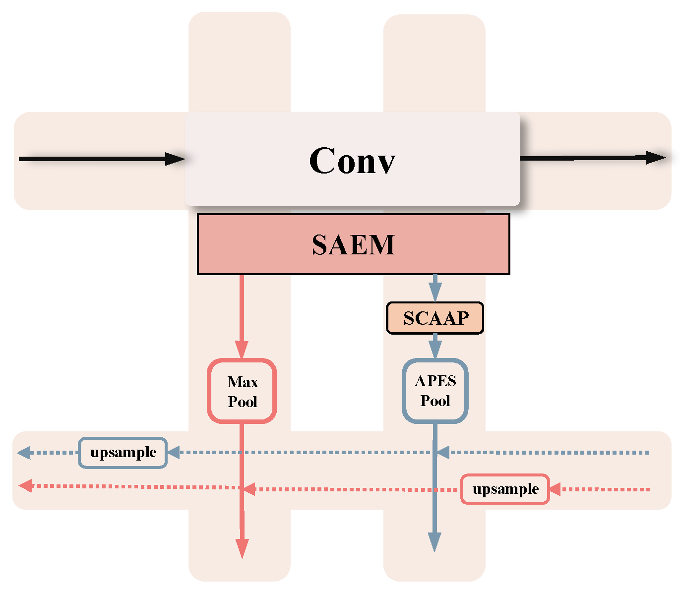
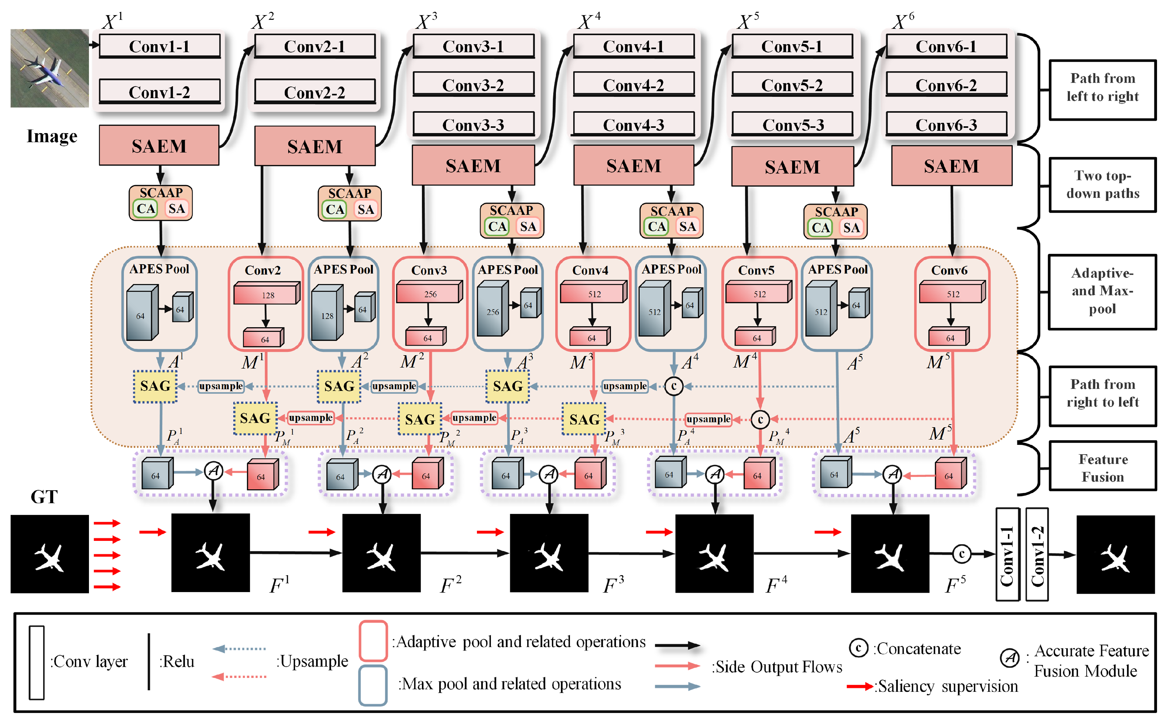
• A convolutional path (left to right) for hierarchical feature extraction;
• A pooling path (top to bottom) combining max and adaptive pooling to adjust receptive fields;
• An up-sampling path (right to left) for reconstructing high-resolution saliency maps.

This grid-like design enables effective local-global feature fusion and preserves fine details. At its core, the SCAAP module combines spatial and channel attention with adaptive pooling, allowing dynamic focus on important regions. This is especially effective in complex scenes and small-object detection, addressing the limitations of conventional pooling in maintaining boundary integrity and saliency.

The design of IEAM-Net integrates three key innovations:

• SCAAP module and adaptive pooling strategy;
  IEAM-Net introduces the SCAAP module, which combines adaptive pooling and channel attention to dynamically adjust pooling sizes and focus on salient areas. Unlike traditional pooling methods, this module better handles multi-target and small-object detection, especially in preserving boundaries and saliency.
• Multi-path feature extraction of Tic-Tac-Toe structure;
  The tic-tac-toe structure is used for grid pooling, which includes a left-to-right convolution path, a top-to-bottom pooling path, and a right-to-left up-sampling path to achieve multi-path feature extraction of Figure 2. Through this multi-level information fusion method, IEAM-Net can capture multi-scale features and improve the detail retention ability of target detection, especially in complex backgrounds and different scale target detection tasks.
• Enhance edge perception and spatial adaptability.
  IEAM-Net incorporates two key modules: SAEM (Spatially Adaptive Edge Embedded Module) and the SAG-Model (spatial adaptive guidance module). SAEM enhances edge detection using multi-scale convolution, while the SAG-Model fuses weighted multi-scale features with spatially guided convolution to better focus on key regions. Together, they improve boundary accuracy and spatial feature extraction for salient target detection.

3. Proposed Method

In this section, we first introduce the general structure of IEAM-Net. We will detail the structure and functions of the Spatially Adaptive Edge Embedded Module (SAEM) module, the Spatial-Channel Attention Adaptive Pooling Module and its three sub-modules, and introduce the mechanism of bidirectional interactions between the CAAS (Channel Attentive Adjustment Sub-module) and the SAAS (Spatial Attentive Adjustment Sub-module) to optimize the feature weights as well as the SAG-Model (Spatial Adaptive Guidance Module). To facilitate more precise feature weighting, we design a bidirectional attention interaction mechanism consisting of two sub-modules: Channel Attention Adjustment Sub-module (CAAS), which emphasizes informative feature channels by learning inter-channel dependencies through global average pooling and fully connected layers; and Spatial Attention Adjustment Sub-module (SAAS), which enhances salient spatial locations by capturing spatial-wise importance through convolutional operations on aggregated feature maps. These two sub-modules interact recursively to refine each other’s attention distribution: CAAS guides SAAS to focus on spatial regions supported by strong channel cues, while SAAS reinforces CAAS by spatially modulating the contribution of channels. This mutual reinforcement strategy allows the network to adaptively recalibrate attention maps across both dimensions. Finally, we propose an accurate feature fusion module to integrate features from different paths, which effectively improves the target detection accuracy, and a deep supervised mechanism to enhance the supervised learning process of IEAM-Net by optimizing the network training through multi-level loss.

3.1. Network Framework

Figure 3 illustrates the overall structure of the IEAM-Net for salient target detection. The network takes the entire image I (top left) as input and produces the final salient map P as the output. IEAM-Net follows a U-Net-like architecture consisting of a left-to-right convolutional path, two top-down paths (max pooling and adaptive pooling), and a right-to-left up-sampling path. This design, highlighted in the first and second parts of Figure 3, allows for the fusion of multiple levels of sub-features, capturing complex details that are otherwise difficult to obtain.

The architecture is based on several key components:

SAEM Module: The Spatial-Aware Edge Module (SAEM) processes edge information and extracts key features through multi-scale convolutions.

Spatial-Channel-Attentive Adaptive Pooling Module: Positioned at the center of the tic-tac-toe structure, this module captures features from multi-level complementary contexts. It uses up-down convolutions to refine features along the left-to-right path in a fine-grained manner.

SAG-Model: The Spatial Adaptive Guidance Model (SAG-Model) enhances spatial details of the image features.

Feature Fusion Module: This module combines local spatial structures with salient regions, resulting in the final output map for salient target detection.

• Left-to-Right Pathway;
  The left-to-right pathway, adapted from VGG-16, is used for hierarchical feature extraction through five convolutional blocks (Conv2 to Conv6). Unlike existing approaches, we extract features from the last convolutional layer of each block, instead of pooling, which retains more spatial, channel, and boundary details. The original three fully connected layers of VGG-16 are replaced with three additional convolutional layers (Conv6) to further refine features after Conv5. This results in five multi-scale feature extractions from Conv2-2, Conv3-3, Conv4-3, Conv5-3, and Conv6-3 layers.
• Two Top-Down Paths;
  • Max-Pool Path; The max-pool path begins with higher-level features from the Conv2-2, Conv3-3, Conv4-3, Conv5-3, and Conv6-3 layers. It first passes through a max-pooling layer to downsample the features, extracting higher-level semantic information. As the features move down, they are restored to the appropriate size via up-sampling and fused with features adaptively pooled through the SCAAP module. This is followed by a refinement convolutional block for further feature extraction and a channel transformation layer that adjusts feature channels for fusion.
  • Adaptive Pool Path; The adaptive pool path starts with features from Conv1-2, Conv2-2, Conv3-3, Conv4-3, and Conv5-3, processed by the SCAAP module. The features undergo spatial and channel attention adjustments before pooling, resulting in feature maps with enhanced representation of the salient target regions. These are then fused with the max-pooling features via up-sampling, concatenation, and convolution, ensuring the combined features accurately represent salient target information.
• Right-to-Left Path.
  The right-to-left path refines hierarchical features that have undergone adaptive and max pooling via the SCAAP module, followed by up-sampling. The features, denoted as Ai and Mi, pass through two distinct pooling paths—adaptive and max pooling—and are fused via up-sampling and convolution operations to produce the final predictive features.

In the leftmost and rightmost paths, the features A5 and M5 are directly used as the top predictive features, refined through max-pooling and adaptive pooling, respectively. For the middle layer, features are integrated through bilinear up-sampling, concatenation, and up-convolution operations from the two independent paths to produce the final prediction.

The predictive features $P_A^i$ and $P_M^i$ can be expressed as follows:

$$P_T^i=\left\{\begin{array}{c}{T}^{i}i=5\hfill \\ UpConv\left(cat\left(T^i,Up\left(P_T^{i+1},T^i\right)\right)\right)i\in [1,4]\hfill \end{array}\right.$$

(1)

where T denotes the adaptive pooling path and the maximal pooling path. A denotes the adaptive pooling path and M denotes the maximal pooling path. Up denotes the bilinear up-sampling operation. $T^i$ denotes the refinement features generated by the average and maximal pooling modules as described later. $Up\left(P_T^{i+1},T^i\right)$ denotes up-sampling the feature map from the upper layer to the size of the current layer’s feature map $T^i$ so that the two can be concatenated. The cat operation connects the refinement features at that level with the up-sampled features from the upper layers. Up-Conv denotes the three kernels of 3 × 3 kernel size of the convolutional layer to enhance the robustness of the connected features. For convenience, we abbreviate the convolution parameters.

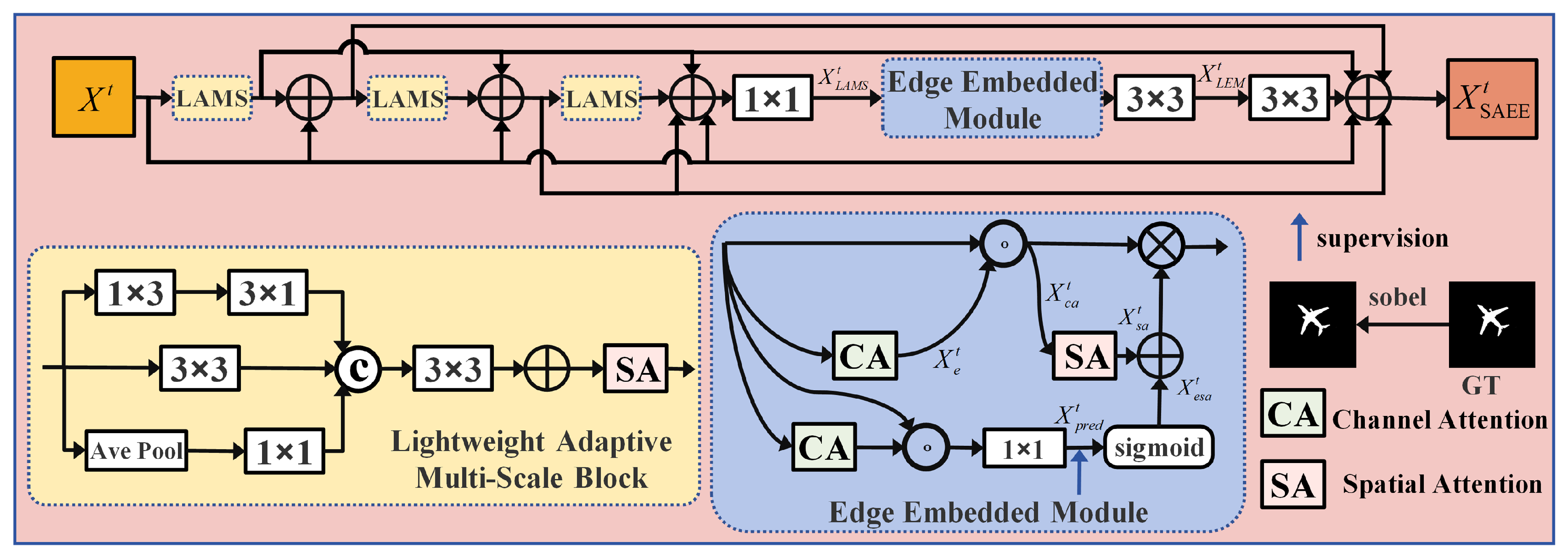
3.2. Structure and Function of the SAEM Module

The Spatially Adaptive Edge Embedded Module (SAEM) is a multi-stage processing module used to process edge information from input images via multi-scale edge enhancement techniques. As shown in Figure 4, the module enhances edge information for input images while considering multiple spatial and contextual relationships within the image, making it adaptive to varying levels of image features. The main components in the SAEM module are the Light Adaptive Multi-Scale (LAM) and Edge Embedding Networks (EEM).

The module operates based on the Region of Spatial Information (RSI), which contains many images with varying levels of details and complexity. In these cases, if the edge information is blurry, it will directly affect the network’s performance. The fast processing of edge-enhanced feature maps helps to focus the network’s attention on these regions, improving both the resolution and accuracy. Therefore, we designed three LAM blocks inside the SAEM module to refine the images with multi-scale features, enhancing its capability to handle images with diverse edge information and improve performance.

3.2.1. LAM (Light Adaptive Multi-Scale Block)

The LAM module provides multi-scale enhancement for input features with different resolutions. Let the input be denoted as X¹. The operation can be expressed as:

$$X_{LAM}^1=\left[\mathrm{Conv}(X^1,1\times 3),\mathrm{Conv}(X^1,3\times 1),\mathrm{Conv}(X^1,3\times 3),\mathrm{Conv}(\mathrm{AvePool}\left(X^1\right),1\times 1)\right]$$

(2)

In the LAM (Lightweight Adaptive Multi-Scale Block), multi-scale contextual features are captured via three parallel branches:

The first branch applies a 1 × 3 convolution followed by a 3 × 1 convolution to extract directional features.The second branch performs a 3 × 3 convolution for standard local feature extraction. The third branch applies average pooling followed by a 1 × 1 convolution to encode global context information.

The outputs of all branches are concatenated along the channel dimension and passed through a 3 × 3 convolution. The number of output channels is adjusted back to 32. An element-wise addition with the input feature map is then performed, followed by a Spatial Attention (SA) module to refine salient features. This architecture allows LAM to expand the receptive field and enhance multi-scale contextual understanding with minimal computation cost.    

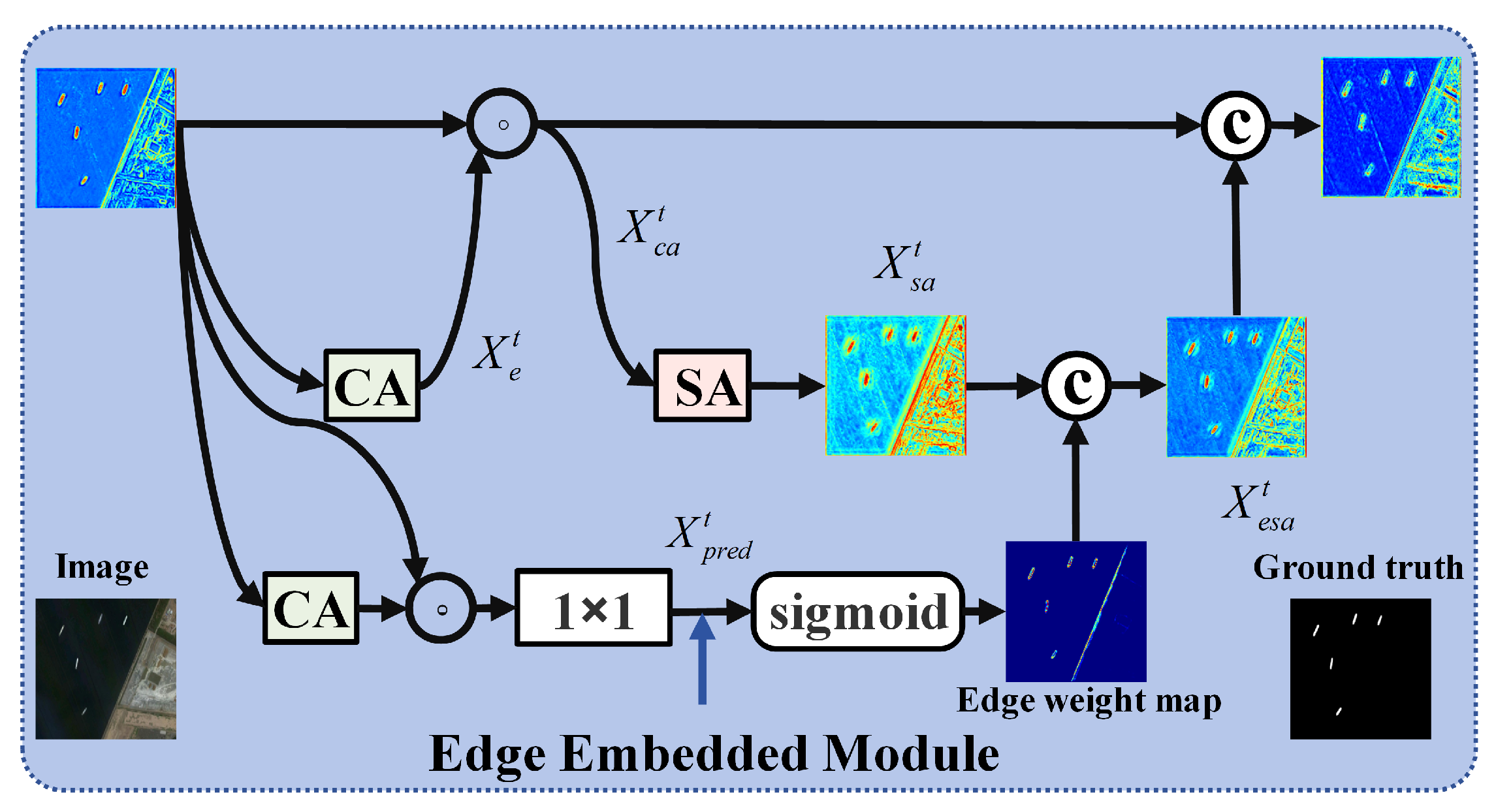
3.2.2. EEM (Edge Embedded Module)

In the Edge Enhancement section, we propose an edge-embedded attention mechanism in order to integrate the edge information into the spatial attention graph to improve the localization accuracy of salient targets. Specifically, we design a new path to learn an edge prediction graph by adding significant edge loss, which extracts the significant edge information from the ground truth image of the salient object through a Sobel filter. This edge prediction map is then combined with channel and spatial attention information to form an edge-embedded attention mechanism to further enhance the model’s ability to perceive edge features.

The purpose of the edge embedding module is to perform edge enhancement of the input image by means of Sobel’s algorithm. Its output is described by the following equation:

$$X_{EM}^1=Sobel\left(X^1\right)\otimes X^1$$

(3)

where ⊗ denotes the element-by-element multiplication operation and the Sobel operator is used to extract the edge information of the image.

As shown in Figure 5, by enhancing the edges of an image, the edge embedding module is able to highlight the contour information of an object, which helps in the recognition and localization of salient targets. Edge information is crucial in vision tasks because edges usually represent structural and semantic information in an image. Conventional convolutional neural networks (CNNs) are usually more limited in the extraction of edge information, whereas by introducing salient edge features through the edge embedding module, the model is able to more accurately localize and identify targets in the image.

The channel attention module generates weights for each channel by global average pooling with the following formula:

$$CA\left(X^1\right)=\sigma \left(W_1·ReLU\left(W_2·AvePool\left(X^1\right)\right)\right)$$

(4)

where $W_1$ and $W_2$ are learnable weight matrices, $\sigma$ is a sigmoid activation function, and Ave-Pool denotes global average pooling. The spatial attention module, on the other hand, focuses on the importance of each spatial location in the image, which is realized by the following equation:

$$SA\left(X^1\right)=\sigma \left(W_3·ReLU\left(W_4·Conv\left(X^1,3\times 3\right)\right)\right)$$

(5)

where $W_1$ and $W_2$ are the learned convolution kernel parameters and Conv denotes the convolution operation.

In the edge embedding module, the channel attention mechanism is used to assign different weights to each channel to highlight the channels that are most critical for target detection. Specifically, the channel attention module computes the average value of each channel through a global average pooling operation to generate a global feature descriptor. This descriptor is tuned by a learnable weight matrix and a sigmoid activation function is used to generate weights for each channel. This operation can dynamically adjust the network’s attention according to the feature importance of different channels, which helps the network to extract the most significant target features among the multi-scale features. After adjusted by channel attention and spatial attention, the input feature maps are fused and output the final prediction results $X_{\mathrm{pred}}^1$, which are fused as follows:

$$X_{\mathrm{pred}}^1=sigmoid\left(\left(X_{CA}^1+X_{SA}^1\right)\otimes X_{EM}^1\right)$$

(6)

where ⊗ is multiplied element by element and finally the sigmoid activation function is used to output the significant target detection results.

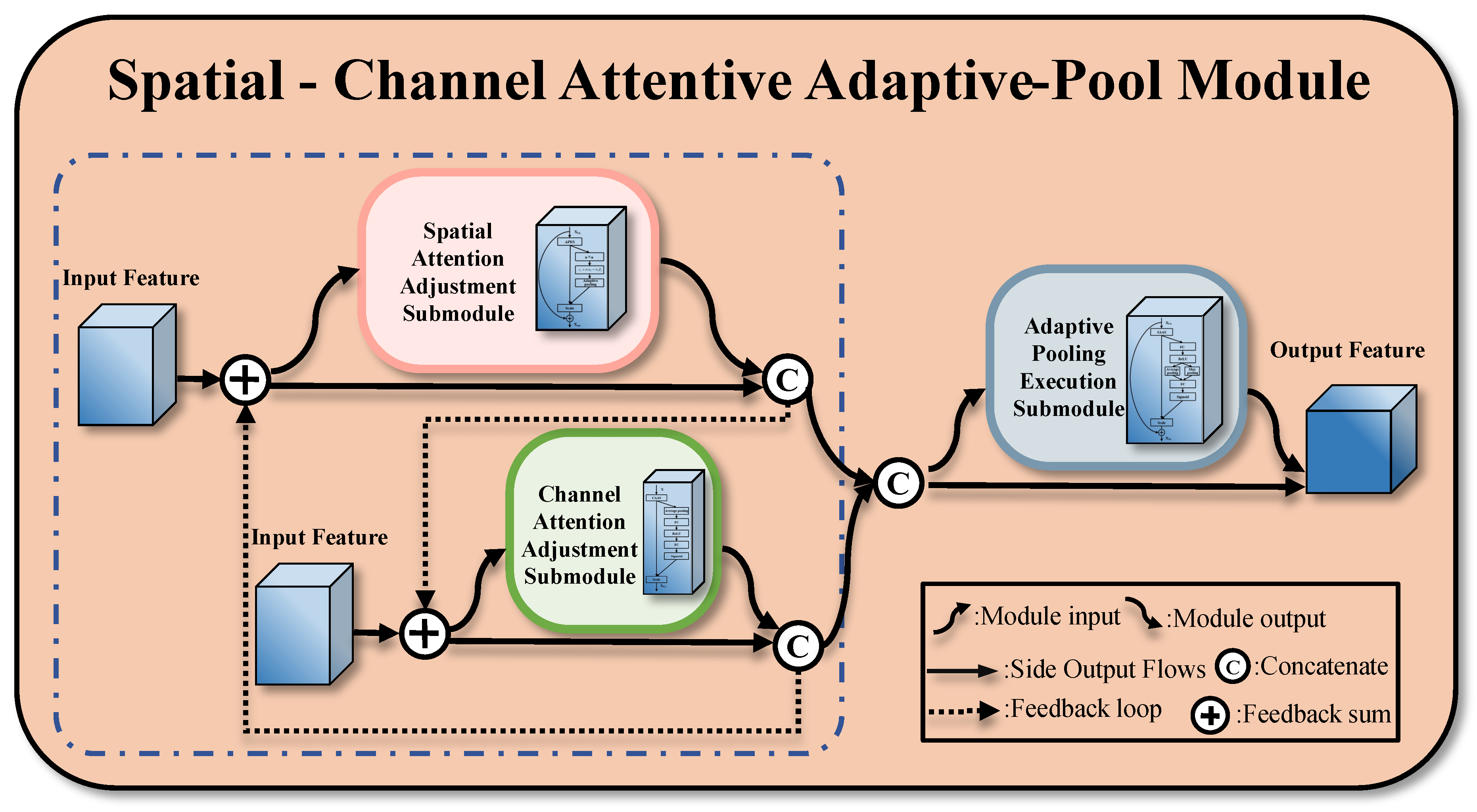
3.3. Spatial-Channel-Attentive Adaptive-Pool

The Spatial-Channel Attention Adaptive Pooling (SCAAP) module is a key point in our proposed network architecture, and the SCAAP module consists of three main sub-modules: the Channel Attention Adjustment Submodule (CAAS): to emphasize important channel features, the Spatial Attention Adjustment Submodule (Spatial Attention Adjustment Submodule (SAAS): highlights important spatial regions, and the Adaptive Pooling Execution Submodule (APES): performs adaptive pooling based on attention weights. It enhances feature representation by combining spatial and channel attention mechanisms. The input feature map first enters the two-way interaction mechanism between CAAS and SAAS, and the core goal of the two-way interaction mechanism is to enhance the feature representation capability of the attention module through the multiple rounds of interactions between the channel attention (CAAS) and the spatial attention (SAAS), so that the two can gradually optimize each other’s weight distribution as shown in Figure 6. In each interaction, Channel Attention helps Spatial Attention focus on more important regions, while Spatial Attention in turn optimizes the selection of Channel Attention, making the final generated attention weights more accurate and robust to adapt to complex scenes and multi-target tasks. The SCAAP pseudocode is as shown in Algorithm 1.

Algorithm 1: Spatial-Channel Attentive Adaptive Pooling (SCAAP)

    Finally, the APES determines the pooling region based on the output of the two-way interaction mechanism and performs the pooling operation to obtain the output feature map. This provides more accurate feature maps for salient target detection. The following is our detailed description of SCAAP module, including the functions, mathematical formulas and parameter settings of each sub-module.

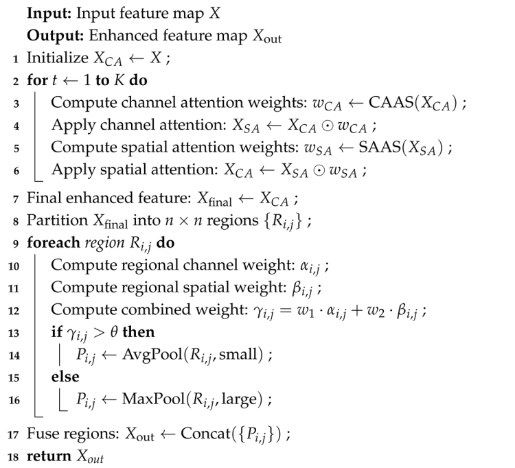
3.3.1. Design Ideas for Two-Way Interaction Mechanisms

The two-way interaction mechanism aims to achieve the following goals through the interaction between channel and spatial attention.

Mutual reinforcement: CAAS provides channel-level attention information to help SAAS focus on more important spatial regions; conversely, the spatial-level attention information provided by SAAS optimizes CAAS’s selection of channel features. Cyclic optimization: Through multiple rounds of interactions, the attention distribution gradually tends to be optimal, and finally outputs more accurate feature representations. Dynamic feedback: The output features of each round of interaction are used as inputs for the next round of computation to dynamically adjust feature selection and attention weights.

Network architecture design: In order to realize the two-way interaction between CAAS and SAAS, this paper adopts the following design.

Step 1: Channel-Space Input feature $X_{input}$. Firstly, through the CAAS module, generate channel attention weight $w_{CA}$: $w_{CA}=CAAS\left(X_{input}\right)$ Use $w_{CA}$ to weight the input feature to get the updated feature $X_{CA}$: $X_{CA}=X_{input}\odot w_{CA}$. Use the updated feature $X_{CA}$ as the input of SAAS.

Step 2: Spatial-Channel Feature $X_{CA}$ passes through the SAAS module, generates spatial attention weight $w_{SA}$:$w_{SA}=SAAS\left(X_{CA}\right)$, weights feature $w_{SA}$ using $X_{CA}$ to get updated feature $X_{SA}$: $X_{SA}=X_{CA}\odot w_{SA}$ inputs updated feature $X_{SA}$ into CAAS again, forming a loop.

Step 3: Multiple Interactions The above two steps form an interaction loop. Repeat the interaction of channel and spatial attention K times ($K=3$), we use 2 rounds in this paper to optimize the attention weights step by step. The formula for the t-th round of multi-round interaction is as follows: $X_{CA}^{\left(t\right)}=X_{SA}^{(t-1)}\odot w_{CA}^{\left(t\right)}$, $X_{SA}^{\left(t\right)}=X_{CA}^{\left(t\right)}\odot w_{SA}^{\left(t\right)}$.

Final Output: After K rounds of interaction, the final output of feature $X_{final}$ is: $X_{final}=X_{SA}^{\left(K\right)}$.

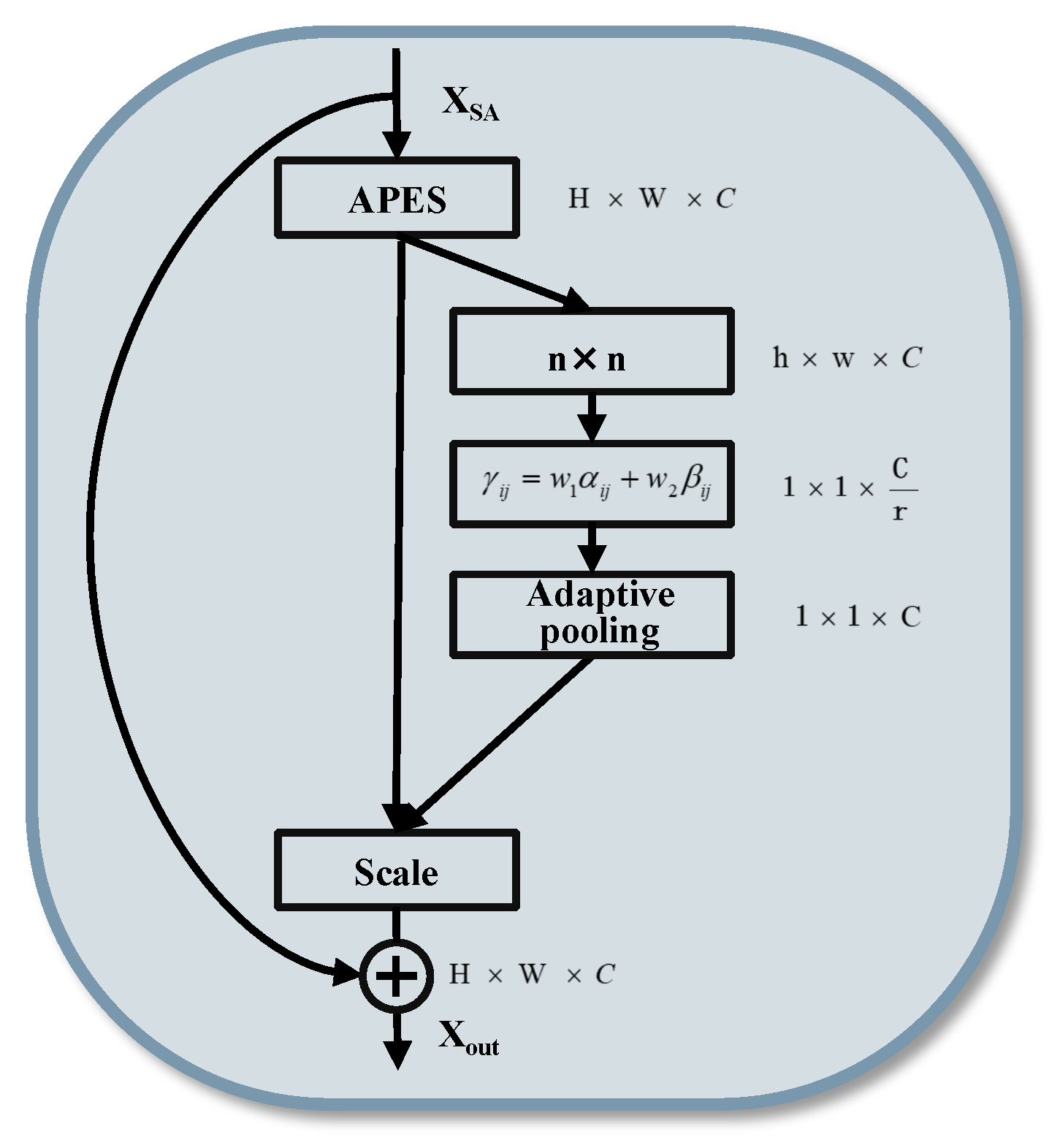
3.3.2. Adaptive Pooling Execution Submodule (APES)

The APES submodule performs adaptive pooling based on the outputs of CAAS and SAAS to integrate the channel and spatial information and generate the final feature map. The spatially attention-adjusted feature map $X_{final}$ is divided into $n\times n$ small regions of equal size (n is flexibly determined based on the size of the input feature map and the desired pooling scale), each of which is of size $h\times w$ (where $h=H/n,w=W/n$) as shown in Figure 7.

For each small region $(i,j)$ $(i=1,2,\dots ,n,j=1,2,\dots ,n)$, compute its integrated attention weight ${\gamma }_{ij}$. The combined attention weight is a combination of the channel attention weight and spatial attention weight in the region, and the weighted summation method is used here, with Equation (7)

$${\gamma }_{ij}=w_1{\alpha }_{ij}+w_2{\beta }_{ij}$$

(7)

where ${\alpha }_{ij}$ is the average of the channel attention weights in the region, ${\beta }_{ij}$ is the average of the spatial attention weights in the region, $w_1$ and $w_2$ are pre-set weighting coefficients.

The size of the pooling region and whether or not to pool are determined based on the combined attentional weights ${\gamma }_{ij}$. If ${\gamma }_{ij}>\theta$ ($\theta$ is a pre-set threshold set to 0.5), a smaller pooling region is used for the region, with average pooling of $h/2\times w/2$. If ${\gamma }_{ij}\le \theta$, a larger pooling region is used for the region, with maximal pooling of $h\times w$

$$P(i,j)=\left\{\begin{array}{cc}{max}_{k,l}{X}^{″}(i,j,k,l)\hfill & \mathrm{if} W(i,j)>\theta \hfill \\ {\displaystyle \frac{1}{k\times k}}{\displaystyle \sum _{m-1}^k}{\displaystyle \sum _{n-1}^k}{X}^{″}(i+m,j+n,:,:)\hfill & \mathrm{otherwise}\hfill \end{array}\right.$$

(8)

Finally, all the small regions that have undergone the pooling operation are recombined to form the output feature map $X_{\mathrm{out}}$.

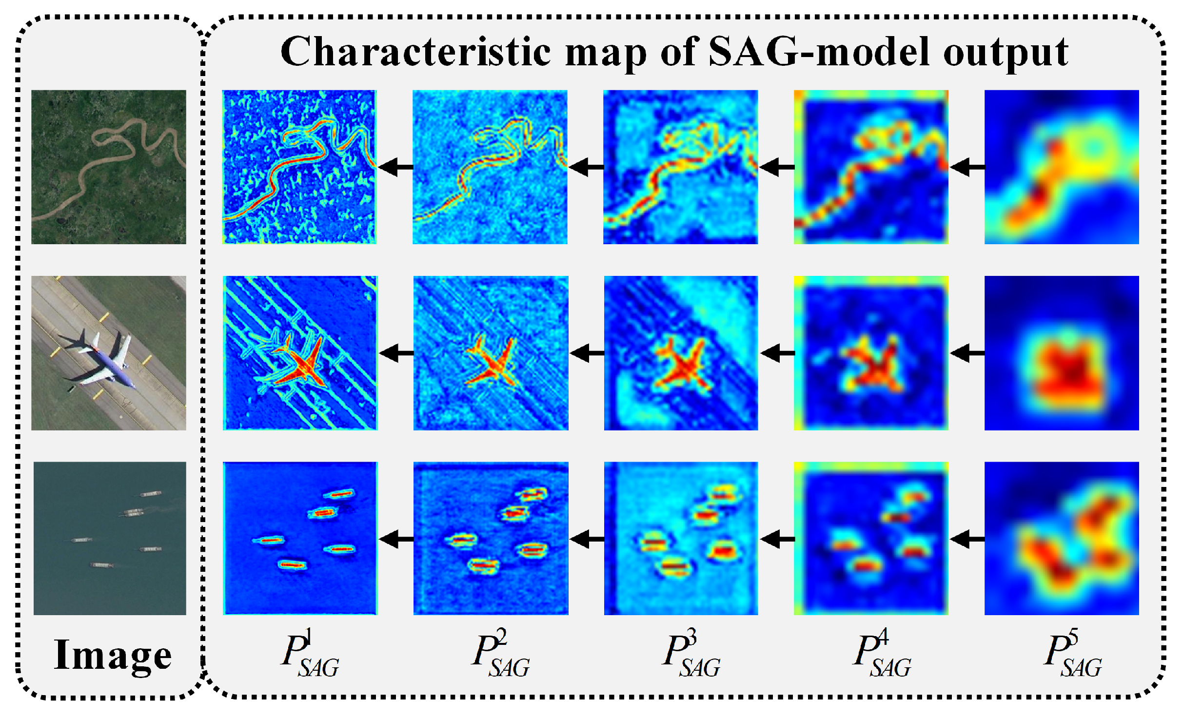
3.4. Structure and Function of the SAG Module

The SAG-Model is mainly used to enhance the spatial adaptation of image features, adaptive pooling paths after SCAAP and maximum pooling paths after the SAEM module to guide the network to better focus on the salient regions in the image. As shown in Figure 8, the core idea of the module is to capture the important spatial information in the image by weighted multi-scale feature maps and spatially guided convolution to improve the accuracy of salient target detection.

SAG-Model receives five input feature maps $P_{T_i}^1,P_{T_i}^2,P_{T_i}^3,P_{T_i}^4,P_{T_i}^5$ (from different layers of the network or multi-scale inputs). These input feature maps are weighted and fused. Each feature map undergoes an element-by-element multiplication operation (⊗) and the contribution of each feature map is adjusted by a weighting factor. The weighted feature maps are fused with spatially guided information to form a more refined feature representation. This process allows the model to dynamically adjust the attention of specific regions in the image according to the importance of different input feature maps. The following equation gives the mathematical expression for weighted fusion:

$$P_{SAG}=\sum _{i=1}^5{\alpha }_i\otimes P_{T_i}^i$$

(9)

where ${\alpha }_i$ is the weighting coefficients of each input feature map, which can be learned by the network. $P_{T_i}^i$ denotes the ith feature map. ⊗ denotes the element-by-element multiplication operation.

Next, spatially guided convolutional operations are applied to each feature map. The spatial information is extracted and enhanced by a 3 × 3 convolution kernel that performs a convolution operation on each input feature map. This spatially guided convolution operation not only extracts fine-grained spatial features in the image, but also enhances the spatial structure of objects in the image. This weighted fusion process ensures that information at different scales and with different features is effectively fused for subsequent spatial guidance. The following equation expresses the process of spatially guided convolution:

$$P_{SAG,\mathrm{conv}}=Conv\left(P_{SAG},3\times 3\right)$$

(10)

The manipulation helps to enhance the spatial structure, allowing the model to more accurately capture salient areas in the image. The SAG pseudocode is as as shown in Algorithm 2.

Algorithm 2: Spatial Adaptive Guidance (SAG)

The fusion process is one of the core steps of SAG-Model. In this process, all the spatially guided convolutionally enhanced feature maps are further fused. A 1 × 1 convolutional layer is used in the fusion operation, which can effectively combine the information from different scales and channels to produce the final output feature maps. Through this fusion method, the SAG-Model integrates the spatial information and details of different feature maps to generate a more adaptive feature map, which provides more accurate inputs for subsequent target detection tasks. The following equation describes this fusion process:

$$P_{SAG}=Conv\left(\left[P_{T_i,\mathrm{conv}}^1,P_{T_i,\mathrm{conv}}^2,P_{T_i,\mathrm{conv}}^3,P_{T_i,\mathrm{conv}}^4,P_{T_i,\mathrm{conv}}^5\right],1\times 1\right)$$

(11)

Finally, the spatially guided and convolutionally fused feature maps $P_{SAG}$ are passed as output to the subsequent target detection network as shown in Figure 9. This output feature map not only contains accurate spatial guidance information, but also ensures that the network can focus on key regions in the image through weighting and multi-scale feature fusion, which improves the detection performance of significant targets.

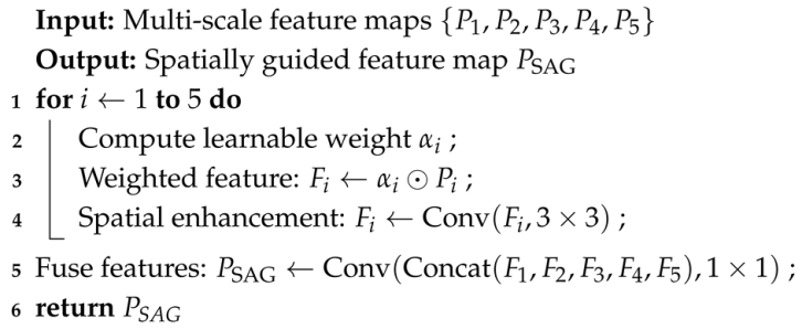
3.5. Accurate Feature Fusion Module

Our proposed network structure is complementarily sampled from maximum pool channels and adaptive pool channels, which are adaptively pooled according to the channel and spatial attention under the SC-AAP module to focus more on the detail features and locally important regions of salient targets. In order to accurately locate the detail features and locally important regions of the salient images in the picture, after sampling, we then propose the accurate feature fusion module maximally adapted to the multi-channel sampling network structure, with the aim of integrating the feature information from two different paths, improving the model’s ability to detect the salient targets and the accuracy of the feature representation. The following describes the accurate feature fusion module specifically.

3.5.1. Feature Adaptation and Fusion

Firstly, before feature fusion, we convolve $F_{max}$ to adjust the number of channels so that it is the same as that of $F_{adaptive}$. This step ensures that the two feature maps can be effectively weighted and summed in the channel dimension in the subsequent feature fusion operation. The adjusted feature map $F_{max}^{\prime }$ is computed as:

$$F_{max}^{\prime }=Conv\left(F_{max},W_1,b_1\right)$$

(12)

where $W_1\in R^{k_1\times k_1\times C_{max}\times C_{\mathrm{adaptive}}}$ is the weight matrix of the convolutional layer, $C_{max}$ is the original number of channels of $F_{max}$ and $b_1\in R^{H\times W}$ is the bias vector, we then, we adopt the multi-scale balancing mechanism approach to fuse the adjusted feature maps $F_{max}^{\prime }$ and $F_{adaptive}$. A learnable weight parameter $\omega$ is introduced, and the fusion weights of the two channels’ features are dynamically adjusted according to the mean values by calculating the global means $\mu \left(F_{\max }^{\prime }\right)$ and $\mu \left(F_{\mathrm{ada}}\right)$ of $F_{\max }^{\prime }$ and $F_{\mathrm{ada}}$. The specific calculation process is as follows.

$$\omega =\sigma \left(W_{\mathrm{bal}}·\left[\mu \left(F_{{max}^{\prime }}\right),\mu \left(F_{\mathrm{ada}}\right)\right]+b_{\mathrm{bal}}\right)$$

(13)

where $\sigma$ is the Sigmoid activation function. In Equation (12), $F_{max}^{\prime }$ and in Equation (13), $F_{\mathrm{ada}}$ are intermediate feature maps used before feature fusion. They are adaptively fused based on a learned weight parameter $\omega$, which is computed from their global mean values. The result of this fusion serves as an input to the spatially guided fusion module, which ultimately produces the final output feature map $P_{SAG}$ in Equation (11).

Therefore, $F_{max}^{\prime }$ and $F_{\mathrm{ada}}$ are important intermediate features that contribute to generating, $P_{SAG}$ which is the spatially guided and convolutionally fused feature map used for improved target detection performance. The fused feature map $F_{fused}$ is calculated as:

$$F_{\mathrm{fised}}=\omega F_{{max}^{\prime }}+(1-\omega )F_{\mathrm{adaptive}}$$

(14)

During the training process, the model automatically learns to adjust these weight parameters to determine the relative importance of the two input feature maps in the fusion process.

3.5.2. Feature Compression and Up-Sampling

Although the fused feature map synthesizes the information from the two inputs, it may have redundancy or an excessive number of channels, which is not conducive to subsequent processing. Therefore, a more compact feature representation is obtained by reducing its number of channels to an appropriate value through a convolutional compression operation. In order to reduce the amount of computation and obtain a more compact feature representation, a convolutional compression operation is performed on the fused feature map $F_{compressed}$. Then the compressed feature map is computed as:

$$F_{compressed}=Conv\left(F_{fused},W_2,b_2\right)$$

(15)

where $W_2\in R^{k_2\times k_2\times C_{fused}\times C_{compressed}}$ is the weight matrix of the convolutional layer, $C_{fused}$ is the number of original channels of $F_{fused}$, $b_2\in R^{Compressed}$ is the bias vector, and finally, we perform an up-sampling operation on the compressed feature map $F_{compressed}$ to restore its size to match the input image to obtain the final output feature map $F_{out}$. The bilinear interpolation up-sampling method is used, and the up-sampling multiplier is determined according to the change of the feature map size in the network, let the up-sampling multiplier be, then the up-sampling operation formula is:

$$F_{out}=Upsample\left(F_{compressed},r\right)$$

(16)

The accurate feature fusion module effectively integrates feature information from two different paths through a carefully designed and fused process, improving the model’s ability to detect salient targets and the accuracy of feature representation.

3.5.3. Deep Supervision Mechanism

In order to optimize our network efficiently, we introduce a deep supervision mechanism, which obtains a multi-level feature representation of the network through multi-level branching outputs and saliency maps. During the training process, we gradually optimize the training parameters of the network by monitoring these intermediate outputs and calculating their cross-entropy losses. The specific loss function can be expressed as.

$$l=-{\displaystyle \frac{1}{W\times H}}\sum _{x=1}^W\underset{y=1}{\sum ^H}[G(x,y)log\left(S(x,y)\right)+(1-G(x,y))log(1-S(x,y))]$$

(17)

where $G(x,y)$ and $S(x,y)$ denote the label value and predicted significance value of a pixel $(x,y)$, respectively, and W and H are the width and height of the input image, respectively. This loss function facilitates the network’s accurate identification of salient regions at all scales by comparing the prediction of each pixel with its true label.

To further improve the performance of the network, we combine the losses from the multi-level branching outputs of the three paths (adaptive pooling path, maximum pooling path, and the fusion of the two) during the training process. The final training loss is defined as the weighted sum of these losses with the following equation.

$$L=\sum _{i=1}^6{\alpha }_i\left(l_A^i+l_M^i+l_{AM}^i\right)$$

(18)

where L is the total network loss, i denotes the different multi-level branch outputs and significance maps (6 branches in total), and ${\alpha }_i$ is the weight of each branch output loss, which takes the following values:

$${\alpha }_i=\left\{\begin{array}{cc}1,\hfill & i=6\hfill \\ 2-i,\hfill & i=5,4,3,2,1\hfill \end{array}\right.$$

(19)

The design of the deep supervision mechanism helps the network to self-regulate and optimize from multiple scales and paths. With this multi-level supervision, the network is able to better capture the details of salient objects in the image while avoiding the limitations associated with single-path supervision. In addition, this mechanism allows the network to obtain more gradient information during training, which accelerates convergence and improves performance.

In the comparative experiments in this paper, we also introduced a non-deep supervision mechanism (single-path supervision) to evaluate the effectiveness of the deep supervision mechanism, further demonstrating the advantages of deep supervision in the saliency detection task. Through these experiments, we are able to more comprehensively verify the contribution of the SCAAP module at different levels and paths, and provide theoretical support for further optimization.

4. Experimental Results and Analysis

4.1. Experimental Setup

4.1.1. Datasets

We use two public optical remote sensing image datasets, ORSSD [8] and EORSSD [7], to thoroughly validate our model. The ORSSD dataset contains 800 images, with 600 used for training and 200 for testing. It features diverse spatial resolutions, object scales, types, and cluttered backgrounds. The EORSSD dataset, an extension of ORSSD, contains 2000 images, with 1400 for training and 600 for testing. Both datasets include pixel-level annotations for each image.

In our experiments, we train the model using 600 images from ORSSD and 1400 from EORSSD, with 200 and 600 images, respectively, used for testing. To expand the training data, we applied rotation (90°, 180°, 270°) and mirror reflection (90°, 180°, 270°) operations, resulting in 4800 training samples for ORSSD and 11,200 for EORSSD. During training, we resized each image to 256 × 256 × 12.

4.1.2. Evaluation Metrics

To quantitatively compare the performance of different salient target detection models on the ORSSD [8] and EORSSD [7] datasets, we use several evaluation metrics: Precision-Recall (PR) curves, F-measure curves, maximum F-measure at different thresholds ($F_{\beta }^{max}$), average F-measure over multiple thresholds ($F_{\beta }^{\mathrm{mean}}$), F-measure with adaptive thresholding ($F_{\beta }^{\mathrm{adp}}$), S-measure ($S\alpha$), maximum E-measure at different thresholds ($E{\xi }^{max}$), average E-measure over multiple thresholds ($E_{\xi }^{\mathrm{mean}}$), E-measure with adaptive thresholding ($E_{\xi }^{\mathrm{adp}}$), and mean absolute error (MAE) ($\mathcal{M}$).

Precision and recall are standard performance metrics. In our experiments, we calculate 256 pairs of mean precision and recall values at thresholds ranging from 0 to 255 and plot PR curves, with precision on the vertical axis and recall on the horizontal axis. The closer the PR curve is to the (1, 1) point, the better the model’s performance.

F-measure, a composite metric, is the harmonic mean of precision and recall, calculated as follows:

$$F_{\beta }={\displaystyle \frac{\left(1+{\beta }^2\right)\cdot \mathrm{Precision}\cdot \mathrm{Recall}}{{\beta }^2\cdot \mathrm{Precision}+\mathrm{Recall}}}$$

(20)

where $\mathrm{Precision}={\displaystyle \frac{TP}{TP+FP}}$, TP is the number of true cases, FP is the number of false-positive cases, $\mathrm{Recall}={\displaystyle \frac{\mathrm{TP}}{\mathrm{TP}+\mathrm{FN}}}$, FN is the number of false-negative cases. $\beta$ is the balancing factor ($\beta$ is set to 0.3 in the experiments in this paper to focus more on the accuracy rate). Our experiments provide maximum F-measure values, average F-measure values, and adaptive F-measure values, and show the maximum F-measure curves at the same time. The F-measure curves are plotted based on the F-scores and thresholds ([0, 255]), and each F-score is calculated using the above formula at each threshold. The larger the area of coordinates covered by an F-score, the larger the area of coordinates covered by an F-measure curve, and the greater the area of coordinates covered by an F-score. The larger the coordinate area covered by the curve, the better the model performance.

$$\mathcal{M}={\displaystyle \frac{1}{W\times H}}\sum _{x=1}^W\sum _{y=1}^H|S(x,y)-G(x,y)|$$

(21)

where W and H denote the width and height of the saliency map, respectively, $S(x,y)$ is the pixel values of the saliency map, and $G(x,y)$ is the pixel value of the true mask.

The S-measure measures the structural similarity of the saliency map, taking into account both region similarity ($S_r$) and object similarity ($S_o$), and is defined as

$$S_{\alpha }=\alpha ·S_o+(1-\alpha )·S_r$$

(22)

$S_o$ is Object-aware S-measure, which measures the totality of saliency objectives. $S_r$ is Region-aware S-measure, which measures the consistency of regional saliency. $\alpha$ is the weighting factor ($\alpha$ set to 0.5 in the experiments of this paper).

The E-measure evaluates the similarity between the predicted saliency map and GT by considering both the local pixel saliency values and the image-level average saliency values, which is calculated as

$$\xi ={\displaystyle \frac{2{\phi }_{GT}{(x,y)}^{\circ }{\phi }_{FM}(x,y)}{{\phi }_{GT}{(x,y)}^{\circ }{\phi }_{GT}(x,y)+{\phi }_{FM}{(x,y)}^{\circ }{\phi }_{FM}(x,y)}},E_{\xi }={\displaystyle \frac{1}{W\times H}}\sum _{x=1}^W\sum _{y=1}^{H}f\left(\xi \right)$$

(23)

where $f(\cdot )$ is a convex function denoting the Hadamard product, and the alignment matrix $\xi$ is constructed based on the deviation matrices ${\phi }_{GT}$ and ${\phi }_{FM}$, which can be regarded as centering operations on GT and binary salient maps, respectively.

While quantitative metrics such as $F_{\beta }^{\max }$, S-measure, E-measure, MAE, and IoU are widely used to assess model performance, interpreting their practical impact is crucial for understanding model behavior in real-world applications.

Table 1. Qualitative interpretation of standard evaluation metrics in saliency detection.

Metric	What It Measures	Practical Interpretation
$F_{\beta }^{\max }$	Trade-off between precision and recall	Higher score means fewer missed objects and reduced false alarms. Even a 0.005 gain indicates noticeable visual improvement in object completeness and fewer background activations.
S-measure	Structural similarity of prediction vs. GT	Captures how well object shapes and contours are preserved, important for elongated/irregular targets.
E-measure	Enhanced alignment of prediction and GT	Measures consistency in spatial and holistic saliency. A higher E-measure implies better edge connectivity and less spatial fragmentation.
MAE	Pixel-wise average error	Indicates how “clean” the prediction is—lower values reflect smoother backgrounds and fewer fuzzy edges.
IoU	Spatial overlap with ground truth	Reflects how well the predicted and true salient regions match, critical for spatial accuracy.

summarizes the functional meaning of each metric and how typical improvements reflect in qualitative outcomes.

For example, as shown in

Table 2. This table presents a comparative performance analysis of IEAM-Net with 21 advanced SOD (Salient Object Detection) methods across four categories on the EORSSD [7] and ORSSD [8] datasets. The symbols ↑ and ↓ indicate that a larger or smaller score is better, respectively.

Methods	EORSSD								ORSSD
	${\mathit{S}}_{\mathit{\alpha }}\mathbf{\uparrow }$	${\mathit{F}}_{\mathit{\beta }}^{\mathbf{max}}\mathbf{\uparrow }$	${\mathit{F}}_{\mathit{\beta }}^{\mathbf{mean}}\mathbf{\uparrow }$	${\mathit{F}}_{\mathit{\beta }}^{\mathbf{adp}}\mathbf{\uparrow }$	${\mathit{E}}_{\mathit{\xi }}^{\mathbf{max}}\mathbf{\uparrow }$	${\mathit{E}}_{\mathit{\xi }}^{\mathbf{mean}}\mathbf{\uparrow }$	${\mathit{E}}_{\mathit{\xi }}^{\mathbf{adp}}\mathbf{\uparrow }$	$\mathcal{M}\mathbf{\downarrow }$	${\mathit{S}}_{\mathit{\alpha }}\mathbf{\uparrow }$	${\mathit{F}}_{\mathit{\beta }}^{\mathbf{max}}\mathbf{\uparrow }$	${\mathit{F}}_{\mathit{\beta }}^{\mathbf{mean}}\mathbf{\uparrow }$	${\mathit{F}}_{\mathit{\beta }}^{\mathbf{adp}}\mathbf{\uparrow }$	${\mathit{E}}_{\mathit{\xi }}^{\mathbf{max}}\mathbf{\uparrow }$	${\mathit{E}}_{\mathit{\xi }}^{\mathbf{mean}}\mathbf{\uparrow }$	${\mathit{E}}_{\mathit{\xi }}^{\mathbf{adp}}\mathbf{\uparrow }$	$\mathcal{M}\mathbf{\downarrow }$
RRWR	0.5994	0.3993	0.3686	0.3344	0.6894	0.5943	0.5639	0.1677	0.6835	0.5590	0.5125	0.4874	0.7649	0.7017	0.6949	0.1324
HDCT	0.5978	0.5407	0.4018	0.2658	0.7861	0.6376	0.5192	0.1088	0.6197	0.5257	0.4235	0.3722	0.7719	0.6495	0.6291	0.1309
SMD	0.7106	0.5884	0.5475	0.4081	0.7692	0.7286	0.6416	0.0771	0.7640	0.6692	0.6214	0.5568	0.8230	0.7745	0.7682	0.0715
RCRR	0.6007	0.3995	0.3685	0.3347	0.6882	0.5946	0.5636	0.1644	0.6849	0.5591	0.5126	0.4876	0.7651	0.7021	0.6950	0.1277
DSS	0.7868	0.6849	0.5801	0.4597	0.9186	0.7631	0.6933	0.0186	0.8262	0.7467	0.6962	0.6206	0.8860	0.8362	0.8085	0.0363
RADF	0.8179	0.7446	0.6582	0.4933	0.9130	0.8567	0.7162	0.0168	0.8259	0.7619	0.6856	0.5730	0.9130	0.8298	0.7678	0.0382
R3Net	0.8184	0.7498	0.6312	0.4165	0.9483	0.8294	0.6462	0.0171	0.8141	0.7456	0.7386	0.7379	0.8913	0.8681	0.8887	0.0399
EGNet	0.8601	0.7880	0.6967	0.5379	0.9570	0.8775	0.7566	0.0120	0.8721	0.8332	0.7500	0.6452	0.9731	0.9013	0.8226	0.0216
PoolNet	0.8207	0.7545	0.6406	0.4613	0.9292	0.8193	0.6836	0.0210	0.8403	0.7706	0.6999	0.6166	0.9343	0.8650	0.8124	0.0358
GCPA	0.8869	0.8347	0.7905	0.6721	0.9524	0.9167	0.8647	0.0102	0.9026	0.8687	0.8433	0.7861	0.9509	0.9341	0.9205	0.0168
ITSD	0.9050	0.8523	0.8271	0.7421	0.9556	0.9407	0.9103	0.0106	0.9050	0.8735	0.8502	0.8068	0.9601	0.9482	0.9335	0.0165
MINet	0.9040	0.8344	0.8174	0.7705	0.9442	0.9346	0.9243	0.0093	0.9040	0.8761	0.8574	0.8251	0.9545	0.9454	0.9423	0.0144
GateNet	0.9114	0.8566	0.8224	0.7109	0.9610	0.9385	0.8909	0.0095	0.9186	0.8871	0.8679	0.8229	0.9664	0.9538	0.9427	0.0137
U2Net	0.9199	0.8732	0.8329	0.7221	0.9649	0.9373	0.8989	0.0076	0.9162	0.8738	0.8492	0.8038	0.9532	0.9387	0.9326	0.0166
PAKRN	0.9192	0.8639	0.8358	0.7993	0.9616	0.9536	0.9416	0.0104	0.9239	0.8890	0.8727	0.8548	0.9680	0.9620	0.9579	0.0139
SUCA	0.8988	0.8229	0.7949	0.7260	0.9520	0.9277	0.9082	0.0097	0.8989	0.8484	0.8237	0.7748	0.9584	0.9400	0.9194	0.0145
CMC	0.5798	0.3268	0.2692	0.2007	0.6803	0.5894	0.4890	0.1057	0.6033	0.3913	0.3454	0.3108	0.7064	0.6417	0.5996	0.1267
SMFF	0.5401	0.5176	0.2992	0.2083	0.7744	0.5197	0.5014	0.1434	0.5312	0.4417	0.2684	0.2496	0.7402	0.4920	0.5676	0.1854
LVNet	0.8630	0.7794	0.7328	0.6284	0.9254	0.8801	0.8445	0.0146	0.8815	0.8263	0.7995	0.7506	0.9456	0.9259	0.9195	0.0207
EMFINet	0.9290	0.8720	0.8508	0.7984	0.9711	0.9604	0.9501	0.0084	0.9366	0.9002	0.9504	0.8617	0.9737	0.9671	0.9654	0.0109
DAFNet	0.9166	0.8614	0.7845	0.6427	0.9861	0.9291	0.8446	0.0060	0.9191	0.8928	0.8511	0.7876	0.9771	0.9539	0.9360	0.0113
Ours	0.9308	0.8905	0.8473	0.8027	0.9737	0.9625	0.9563	0.0071	0.9421	0.9135	0.8856	0.8947	0.9783	0.9742	0.9663	0.0098

, IEAM-Net improves $F_{\beta }^{\max }$ by 0.005–0.012 compared to strong baselines. While these differences appear small numerically, they correspond to visible qualitative improvements such as: (i) better object boundary integrity, (ii) more accurate exclusion of noisy background, and (iii) higher continuity across occluded targets. These enhancements are observable in visual examples (e.g., Figure 12, row 3 vs. row 6), and are particularly meaningful in downstream tasks like urban analysis or change detection.

Therefore, the metric improvements are both statistically and visually significant, validating the real-world effectiveness of our model.

4.1.3. Implementation Details

Our model was implemented using PyTorch 1.13 and trained on a workstation equipped with an NVIDIA RTX 3090 GPU (24 GB VRAM), an Intel i9 CPU, and 128 GB RAM. We used the Adam optimizer with an initial learning rate of 1 × 10⁻⁴, and adopted a cosine annealing learning rate schedule with a warm-up over the first 5 epochs. The network was trained for 100 epochs with a batch size of 8, using Binary Cross-Entropy loss combined with a deep supervision mechanism. The total training time was approximately 11 h on the EORSSD dataset and 5.5 h on the ORSSD dataset. All experiments were conducted under CUDA 11.6 and Python 3.9 environments.

4.2. Comparison Experiments (With Advanced Methods)

Comparing with 21 state-of-the-art SOD methods, we classify these 21 methods into four categories: the first category is natural scene image SOD methods based on classical vision algorithms (HDCT [35], RCRRS [36], SMD [37], RRWR [38]), the second category is natural scene image SOD methods based on convolutional neural networks (R3Net [11], DSS [39], RADF [40], EG-Net [41], GCPA [34], Pool-Net [18], PA-KRN [42], ITSD [29], Gate-Net [28], SUCA [43], MI-Net [44], U2Net [45]), the third category is for remote sensing image-SOD methods based on classical vision algorithms (CMC [46], SMFF [33]), and the fourth category is for remote sensing image-SOD methods based on convolutional neural networks (LV-Net [7], EMFI-Net [17], DAF-Net [8]). During the experimental process, in order to ensure a fair comparison of the 22 algorithms, we uniformly use the saliency maps provided by the public RSI-SOD benchmark dataset or the saliency maps provided by the authors of the corresponding algorithms, and, for the 7 inside the second category of the above-mentioned convolutional neural network-based SOD methods for natural scene images (ITSD [29], MI-Net [44], Gate-Net [28], GCPA [34], U2Net [45], SUCA [43], PA-KRN [42]), using the same training data to re-train the models on the EORSSD [7] and ORSSD [8] datasets with the default settings provided by the authors.

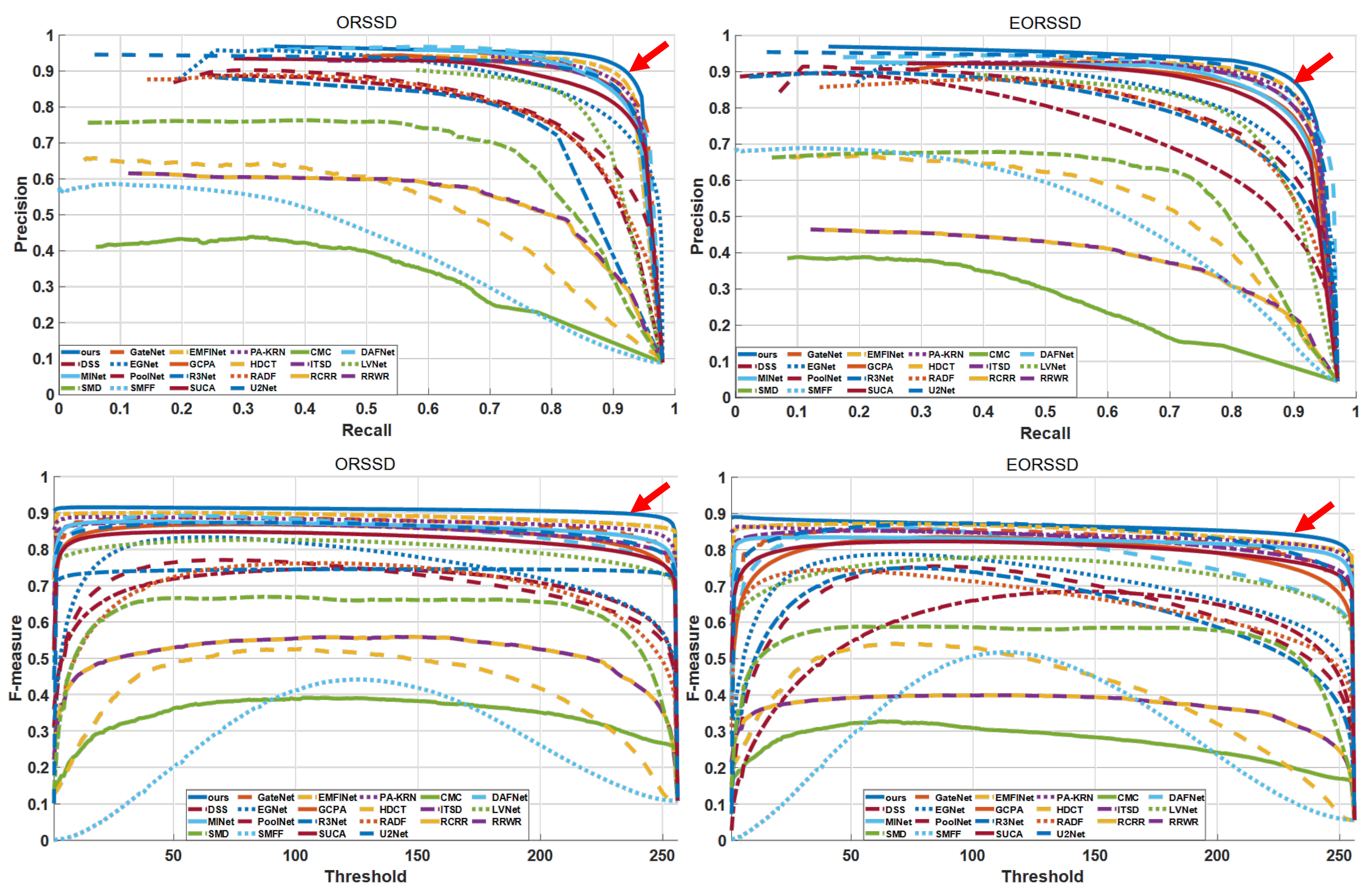
4.2.1. Quantitative Comparison

Table 2 presents a quantitative comparison between IEAM-Net and 21 advanced SOD methods on the EORSSD [7] and ORSSD [8] datasets. The comparison includes traditional and CNN-based SOD methods for both natural and remote sensing images. All methods were evaluated under uniform conditions using saliency maps from the public RSI-SOD dataset or those provided by the authors.

On the EORSSD [7] dataset, IEAM-Net outperforms many methods on several metrics. It achieves 0.9308 on Fmax, surpassing DAF-Net (0.9166) and approaching EMFI-Net (0.9290), showing its accuracy in salient target detection. IEAM-Net also performs well on F-mean with a score of 0.8905, higher than DAF-Net’s 0.8614, demonstrating its stability. For E-max and E-mean, IEAM-Net scores 0.9737 and 0.9625, slightly below DAF-Net’s 0.9861 and 0.9291, but still strong, particularly in complex scenes. Compared to other CNN-based remote sensing image SOD methods (e.g., EMFI-Net and DAF-Net), IEAM-Net excels in metrics like F-adp and M, showing an all-around improvement across multiple evaluation metrics.

Overall, IEAM-Net outperforms most existing methods on the EORSSD [7] dataset, especially in Fmax and F-mean, demonstrating its superiority in salient target detection in remote sensing images. The PR curve (Figure 10) further supports these results, with IEAM-Net’s curve closer to the upper-right corner, indicating excellent performance.

4.2.2. Comparison of Computational Complexity

Computational complexity is typically evaluated based on inference speed (FPS), number of parameters, and floating point operations (FLOPs). Figure 11 provides a comparative analysis of various Salient Object Detection (SOD) methods, including a box plot analysis that further illustrates the distribution and trends of computational efficiency across different approaches. The results demonstrate that IEAM-Net outperforms existing methods in computational efficiency while maintaining high detection accuracy. Most CNN-based methods can run in real-time (16–26 FPS), and IEAM-Net inference speed reaches 48 FPS, which is favorable for practical applications. Its network parameters and FLOPs are at a medium level, compared with the second best EMFI-Net [17], which is 67.65 M (IEAM-Net) less than 107.26 M (EMFI-Net [17]), and the FLOPs are 103.2 G (IEAM-Net) less than 480.9 G (EMFI-Net [17]), which indicates that IEAM-Net is effective and efficient.

Table 3. Comprehensive comparison of IEAM-Net and 21 competing methods on the EORSSD dataset. Metrics include detection accuracy ($F_{\beta }^{\max }$), inference speed (FPS), model size (in millions of parameters), and computational complexity (FLOPs in G). The symbols ↑ and ↓ indicate that a larger or smaller score is better, respectively.

Method	Type	${\mathit{F}}_{\mathit{\beta }}^{\mathbf{max}}$	FPS ↑	Params (M) ↓	FLOPs (G) ↓
RRWR	Traditional	0.3993	5	–	–
UCF	Traditional	0.4521	7	–	–
RBD	Traditional	0.5010	9	–	–
DSS	NSI-CNN	0.6849	22	62.2	130.8
U2Net	NSI-CNN	0.7180	30	44.7	98.5
PoolNet	NSI-CNN	0.7533	22	68.1	150.0
EGNet	NSI-CNN	0.7880	20	94.5	180.6
CPD	NSI-CNN	0.7925	28	47.2	104.3
SCRN	NSI-CNN	0.8010	27	38.7	85.2
MINet	NSI-CNN	0.8127	25	60.3	145.1
ITSD	NSI-CNN	0.8194	24	54.2	131.9
F3Net	NSI-CNN	0.8210	25	52.0	122.4
GCPA	NSI-CNN	0.8347	24	86.7	291.9
PA-KRN	NSI-CNN	0.8639	18	138.3	617.7
DAF-Net	RSI-CNN	0.8614	25	85.4	376.2
DMRA	RSI-CNN	0.8587	20	78.1	330.5
EMFI-Net	RSI-CNN	0.8720	23	107.3	487.3
BLNet	RSI-CNN	0.8704	26	90.2	450.6
RRA-Net	RSI-CNN	0.8673	19	95.0	420.7
CGANet	RSI-CNN	0.8735	21	93.4	412.0
BMNet	RSI-CNN	0.8690	24	81.3	389.6
IEAM-Net (Ours)	RSI-CNN	0.8905	48	67.7	103.2

provides a comprehensive comparison between the proposed IEAM-Net and 21 representative saliency detection methods across three major categories: traditional models, CNN-based models for natural scene images (NSI-CNN), and remote sensing image-specific CNN models (RSI-CNN). The comparison considers four key aspects: accuracy ($F_{\beta }^{\max }$), inference speed (FPS), model size (in millions of parameters), and computational complexity (FLOPs in G).

Notably, IEAM-Net achieves the highest accuracy with an $F_{\beta }^{\max }$ score of 0.8905 while also delivering the fastest inference speed (48 FPS) among all CNN-based models. Despite its strong performance, IEAM-Net maintains a relatively low parameter count (67.7 M) and the lowest FLOPs (103.2 G) in the RSI-CNN category, indicating its superior balance between effectiveness and efficiency.

Compared to recent high-performing methods such as PA-KRN (0.8639 $F_{\beta }^{\max }$, 617.7 G FLOPs) and EMFI-Net (0.8720 $F_{\beta }^{\max }$, 487.3 G FLOPs), IEAM-Net offers not only improved detection accuracy, but also significantly reduced computational cost, making it a practical and scalable choice for real-time remote sensing applications.

Inference Speed Comparison

Most CNN-based SOD methods achieve inference speeds ranging from 16 to 26 FPS, with models such as PoolNet [18], GCPA [34], and PA-KRN [42] maintaining speeds around 24–25 FPS. Traditional methods, including RRWR [38], HDCT [35], SMD [37], and RCRR [36], exhibit significantly lower speeds, often below 10 FPS, highlighting their inefficiency in processing high-resolution remote sensing images. IEAM-Net achieves a remarkable inference speed of 48 FPS, which is nearly twice as fast as the best existing CNN-based methods, including EMFI-Net [17] and DAF-Net [8].

Box plot analysis: The box plot on the left (inference speed) shows that most methods cluster around the lower FPS range (below 26 FPS), with a few high-performing outliers. IEAM-Net is a distinct outlier, achieving a significantly higher speed than the trend observed in other methods, as indicated by the separate data point far above the whiskers. The overall distribution suggests that IEAM-Net significantly deviates from the median speed of existing methods, making it an exceptionally fast approach.

FLOPs Comparison

IEAM-Net significantly reduces computational complexity, requiring only 103.2 G FLOPs, compared to advanced methods like PA-KRN [42] (617.7 G FLOPs), EMFI-Net [17] (487.3 G FLOPs), GCPA [34] (291.9 G FLOPs), and DAF-Net [8] (376.2 G FLOPs). While traditional methods like RRWR [38], HDCT [35], and SMD [37] have low FLOPs, they underperform in detection accuracy. IEAM-Net, with its efficient attention mechanism and adaptive pooling strategy, maintains high precision while minimizing computational cost.

The box plot (FLOPs comparison) shows that most CNN-based SOD methods have high computational costs, with several exceeding 600 G FLOPs (e.g., PA-KRN [42]). IEAM-Net’s FLOPs are well below the median, indicating its competitive performance with lower computational complexity. The varying FLOPs across methods highlight the efficiency of IEAM-Net.

IEAM-Net achieves the highest inference speed (48 FPS), ideal for real-time remote sensing processing. Its FLOPs are 78.8% lower than EMFI-Net [17] (487.3 G) and 83.3% lower than PA-KRN [42] (617.7 G), demonstrating superior computational efficiency. Additionally, with only 67.65 M parameters compared to EMFI-Net’s 107.26 M parameters, IEAM-Net reduces model size by about 37%.

Box plot analysis further confirms IEAM-Net’s exceptional performance in both inference speed and computational efficiency, making it an optimal solution for large-scale remote sensing tasks.

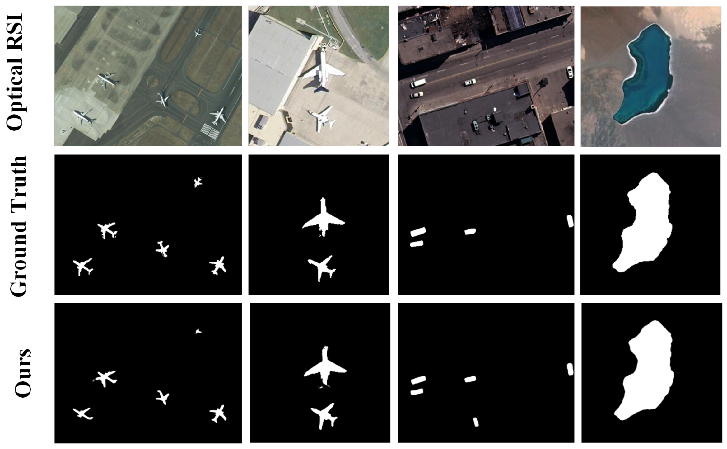
4.2.3. Visual Comparison

Figure 12 compares the performance of IEAM-Net with other salient object detection methods in optical remote sensing images (RSI). It includes various remote sensing scenes, such as airplanes, cars, buildings, rivers, and swimming pools, categorized by conditions such as normal airplanes, airplanes with shadows, and airplanes under disturbances. Each row displays the original optical RSI, the ground truth (GT), IEAM-Net output (highlighted in red), and results from methods like GateNet [28], EMFI-Net [17], PA-KRN [42], U2Net [45], DAF-Net [8], ITSD [29], and RCRR [36].

The results reveal notable performance differences. IEAM-Net detects large objects with complete shapes, while other methods often distort or incompletely segment them. It handles shadows well, maintaining accurate shape detection, unlike other methods that struggle with shadow interference. For multiple objects, IEAM-Net excels at segmentation without merging errors, while some methods fail to detect all objects. In cluttered backgrounds, IEAM-Net distinguishes target objects from noise, whereas other methods suffer from false positives. For small objects, IEAM-Net accurately identifies them, whereas other methods often fail or distort small object shapes. (a) Dense Object Scenes: In urban or port environments (e.g., Figure 12, rows 3 and 5), IEAM-Net accurately distinguishes adjacent targets (e.g., buildings, ships) without boundary merging, thanks to the SAG module’s spatial refinement. (b) Small Target Detection: IEAM-Net captures fine-scale objects such as vehicles and boats (rows 4 and 6), outperforming other methods prone to omission. This benefits from the multi-scale detail retention enabled by SCAAP. (c) Occlusion and Shadow Handling: In partially occluded scenes, our model recovers more complete structures than baselines, owing to its bidirectional attention design that preserves spatial continuity. (d) Cluttered Backgrounds: IEAM-Net exhibits strong background suppression (e.g., over water or vegetation), reducing false positives via edge-aware enhancement (SAEM) and adaptive attention calibration.

Overall, compared to traditional methods (e.g., SMFF [33], SMD [37]), CNN-based non-RSI methods (e.g., PA-KRN [42], U2Net [45]), and CNN-based RSI methods (e.g., EMFI-Net [17], DAF-Net [8], LV-Net [7]), IEAM-Net demonstrates superior accuracy and robustness in optical RSI. Traditional methods struggle with RSI characteristics, CNN-based non-RSI methods face data adaptation issues, and CNN-based RSI methods often produce defective maps. IEAM-Net’s unique design improves object localization and preserves fine contours, proving adaptable and robust in complex environments.

Although IEAM-Net demonstrates strong performance across a wide range of scenarios, several failure cases remain. For instance, as shown in the rightmost columns of Figure 11, the model occasionally fails to detect very small or low-contrast objects, especially when they are heavily occluded by shadows or embedded in cluttered backgrounds. These failures often arise in challenging scenes involving complex textures, overlapping targets, or significant illumination variation, which may mislead the attention modules or cause inconsistencies in feature representation across scales. Common failure patterns include missed detections in occluded or overlapping regions, blurred boundaries in noisy backgrounds, and reduced saliency localization in the presence of densely packed targets. These observations point to limitations in the current model’s ability to balance local-global contextual modeling and maintain fine-grained edge delineation. To address these issues, future work may explore the integration of transformer-based modules to enhance global reasoning, the introduction of multi-resolution fusion mechanisms at earlier network stages, and the design of more advanced edge-preserving or contour-refining loss functions. Additionally, targeted data augmentation strategies that simulate occlusion and noise could further improve the model’s robustness.

4.3. Ablation Experimental Study

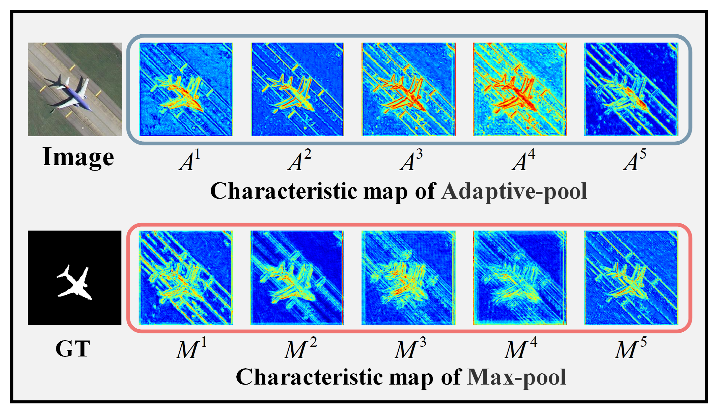
4.3.1. SCAAP Component Ablation Experiments

The effectiveness of the IEAM-Net essential components on the EORSSD [7] and ORSSD [8] datasets was assessed through comprehensive experiments investigating the following aspects: the individual contribution of each content in the SCAAP module, the necessity of merging the original content, and the effectiveness of the combined loss function. Each variant experiment was retrained using the same parameter settings and datasets as in the experimental protocol.

To evaluate the individual contributions of the Spatially Adaptive Edge Embedding Module (SAEM), Spatial Adaptive Guidance Module (SAG), Adaptive Pooling (AP), and Maximal Pooling Path (MP) to the SCAAP module’s performance, we constructed five configurations (top half of

Table 4. This table shows the impact of different module combinations (Baseline, SAEM, SAG, AP, MP) on the performance of IEAM-Net. Fmax $\beta$ and Emax $\xi$ represent the maximum F-score and maximum E-score on the EORSSD [7] and ORSSD [8] datasets, respectively, with arrows indicating that higher values are better.

No.	Baseline	SAEM	SAG	AP	MP	EORSSD		ORSSD
						${\mathit{F}}_{\mathit{\beta }}^{\mathbf{max}}\mathbf{\uparrow }$	${\mathit{E}}_{\mathit{\xi }}^{\mathbf{max}}\mathbf{\uparrow }$	${\mathit{F}}_{\mathit{\beta }}^{\mathbf{max}}\mathbf{\uparrow }$	${\mathit{E}}_{\mathit{\xi }}^{\mathbf{max}}\mathbf{\uparrow }$
1	✓					0.8632	0.9684	0.8878	0.9608
2	✓	✓		✓		0.8817	0.9713	0.9043	0.9721
3	✓		✓	✓		0.8836	0.9727	0.9066	0.9742
4	✓			✓	✓	0.8860	0.9689	0.9086	0.9762
5	✓				✓	0.8842	0.9713	0.9047	0.9718
6	✓	✓		✓		0.8740	0.9623	0.9017	0.9689
7	✓		✓	✓	✓	0.8835	0.9713	0.9126	0.9695
8	✓		✓	✓		0.8872	0.9721	0.9112	0.9723
9	✓	✓		✓	✓	0.8891	0.9702	0.9127	0.9768
10	✓	✓	✓	✓	✓	0.8905	0.9737	0.9135	0.9783

): baseline (VGG-16-based network), baseline + SAEM, baseline + SAEM + SAG, baseline + SAEM + SAG + AP, and baseline + SAEM + SAG + AP + MP.

As shown in Table 4, model performance improves with the progressive addition of modules. The SAEM module enhances channel feature selection, improving detection sensitivity by distinguishing significant regions. The SAG module refines target localization accuracy by capturing key spatial information, making the model more robust in complex scenarios. The AP module adjusts the feature extraction range, enhancing multi-scale salient object handling, while the MP module improves local feature capture, strengthening edge and detail portrayal.

Quantitative results indicate that the full SCAAP module improves performance on the EORSSD [7] dataset from 0.8878 to 0.8905 in the baseline and 0.9096 to 0.9135 overall. On the ORSSD [8] dataset, it improves from 0.8712 to 0.8843 in the baseline, with Emax improving from 0.8995 to 0.9128. The full module’s combined effect improves performance by 2.25% and 1.93%, respectively, highlighting the synergy of SCAAP components.

Additionally, we assessed different module combinations (middle part of Table 4), demonstrating that each module independently boosts performance and that their collaboration further enhances detection. SAEM enhances target edges, SAG improves target area attention, and the combination of AP and MP increases model robustness in multi-scale scenarios. These results validate the effectiveness of the SCAAP module design and its potential for salient object detection in complex scenes.

The image illustrates the impact of adaptive pooling (AP) and max pooling (MP) pathways in IEAM-Net for salient object detection in remote sensing images as shown in Figure 13. The top section shows the original image and feature maps (${\mathrm{A}}^1-{\mathrm{A}}^5$) from the AP pathway, where high-intensity regions highlight the salient target with refined details. AP dynamically adjusts feature extraction, enhancing multi-scale object detection.

The bottom section presents the ground truth (GT) and feature maps (${\mathrm{M}}^1-{\mathrm{M}}^5$) from the MP pathway, which retains overall structure but lacks finer details. While MP ensures global feature consistency, AP provides superior boundary enhancement and noise suppression. The comparison demonstrates that integrating both pooling strategies optimizes detection by balancing detail refinement and structural preservation. This synergy enables IEAM-Net to achieve high-accuracy salient object detection, as validated by ablation study results.

4.3.2. Feature Fusion Module Ablation Experiment

Through this experiment, we deeply validate the importance of fusing raw content in the SCAAP module for accurate feature fusion. Specifically, the experiment evaluates the actual role of fusing raw content in enhancing the effectiveness of saliency detection by comparing two approaches-FFM (traditional feature fusion module) and EAFFM (our proposed improved version of the feature fusion module). As can be seen from the

Table 5. This table compares the performance of the EAFFM (ours) and FFM models on the EORSSD [7] and ORSSD [8] datasets. Fmax $\beta$ and Emax $\xi$ represent the maximum F-score and maximum E-score, respectively, with arrows indicating that higher values are better.

Models	EORSSD		ORSSD
	${\mathit{F}}_{\mathit{\beta }}^{\mathbf{max}}\mathbf{\uparrow }$	${\mathit{E}}_{\mathit{\xi }}^{\mathbf{max}}\mathbf{\uparrow }$	${\mathit{F}}_{\mathit{\beta }}^{\mathbf{max}}\mathbf{\uparrow }$	${\mathit{E}}_{\mathit{\xi }}^{\mathbf{max}}\mathbf{\uparrow }$
FFM	0.8869	0.9717	0.9118	0.9754
EAFFM	0.8905	0.9737	0.9135	0.9783

, the performance of EAFFM compared to FFM on both datasets is significantly improved, proving the effectiveness of fusing raw content.

On the EORSSD [7] dataset, the EAFFM’s improves from 0.8869 to 0.8905, an improvement of 0.0036; and from 0.9717 to 0.9737, an improvement of 0.0020, which indicates that the overall sensitivity and detection effectiveness of the model are significantly enhanced after the introduction of raw content as shown in Table 5.

Similarly, on the ORSSD [8] dataset, the EAFFM improves from 0.9118 to 0.9135 with 0.0017, and from 0.9754 to 0.9783 with 0.0029, which further demonstrates that the fusion of original content can stably improve the model performance on different datasets, especially in the identification of details and edge regions.

These results indicate that fusing raw content not only helps the model to improve the perception of salient regions, but also enhances the robustness of the model, especially in complex scenes. Taken together, the role of original content fusion in accurate feature fusion cannot be ignored, and can effectively compensate for the feature loss and improve the overall accuracy and reliability of detection.

4.3.3. Supervision Mechanism Ablation Experiment

Through this experiment, we further explored the effect of introducing Deep Supervision (Deep Supervision) in the SCAAP module on the model performance enhancement, and compared it with the traditional Single Path Supervision (Single Path Supervision). As can be seen from the data in the

Table 6. This table compares the performance of the DEEP SUP (ours) and SINGLE SUP models on the EORSSD [7] and ORSSD [8] datasets. Fmax $\beta$ and Emax $\xi$ represent the maximum F-score and maximum E-score, respectively, with arrows indicating that higher values are better.

Models	EORSSD		ORSSD
	${\mathit{F}}_{\mathit{\beta }}^{\mathbf{max}}\mathbf{\uparrow }$	${\mathit{E}}_{\mathit{\xi }}^{\mathbf{max}}\mathbf{\uparrow }$	${\mathit{F}}_{\mathit{\beta }}^{\mathbf{max}}\mathbf{\uparrow }$	${\mathit{E}}_{\mathit{\xi }}^{\mathbf{max}}\mathbf{\uparrow }$
SINGLE SUP	0.8875	0.9720	0.9121	0.9769
DEEP SUP	0.8905	0.9737	0.9135	0.9783

, the Deep Supervision mechanism significantly improves the overall performance of the saliency detection task, verifying the effectiveness of multi-scale adaptive adjustment in deep supervision.

On the EORSSD [7] dataset, the model using the deep supervision mechanism (DEEP SUP) improves 0.0030 from 0.8875 to 0.8905 and 0.0017 from 0.9720 to 0.9737 compared to the single-path supervision (SINGLE SUP), and this improvement suggests that the deep supervision mechanism is able to improve the performance of the network from multiple scales through the gradient feedback at multiple levels. feedback, which enables the network to self-optimize from multiple scales and paths, thus enhancing the model’s ability to capture salient regions as shown in Table 6.

On the ORSSD [8] dataset, the deep supervision mechanism also shows significant advantages, from 0.9121 to 0.9135, with an improvement of 0.0014, and from 0.9769 to 0.9783, with an improvement of 0.0014. This result further confirms that the deep supervision mechanism can effectively enhance the robustness of the model in complex scenarios, and accelerate the convergence of the training process.

Through these comparative experiments, we can conclude that the deep supervision mechanism not only enhances the performance of the model in multi-scale scenarios, but also enhances the learning ability of the model through the feedback of the multi-path gradient information, making the network more efficient in the training process. This further proves the unique advantages of the deep supervision mechanism in the saliency detection task.

4.3.4. Impact of Backbone Choice

Although VGG-16 is a widely adopted and stable backbone in the saliency detection literature, it is technically outdated in terms of feature richness, receptive field, and computational efficiency. To assess the impact of backbone selection on the performance of our proposed model, we conducted additional experiments by replacing VGG-16 with two modern architectures:

• ResNet-50: a deeper residual CNN known for its strong semantic representation capabilities.
• EfficientNet-B0: a lightweight yet powerful model that utilizes compound scaling to balance depth, width, and resolution.

Table 7. Performance comparison of IEAM-Net with different backbone networks. The symbols ↑ and ↓ indicate that a larger or smaller score is better, respectively.

Backbone	${\mathit{F}}_{\mathit{\beta }}^{\mathbf{max}}$↑	MAE ↓	FPS ↑	Params (M) ↓
VGG-16 (default)	0.8905	0.031	48	67.7
ResNet-50	0.9072	0.028	42	85.2
EfficientNet-B0	0.8921	0.030	47	59.3

summarizes the performance of IEAM-Net with these three backbones. The ResNet-50 variant achieves a notable increase of +1.7% in $F_{\beta }^{\max }$ while maintaining competitive inference speed. EfficientNet-B0 reduces the total parameter count while achieving comparable accuracy and lower MAE than VGG-16.

These results confirm that IEAM-Net’s core design is robust across different backbones. Nonetheless, employing stronger semantic encoders can yield further improvements in performance. Therefore, in future work, we plan to explore transformer-based backbones (e.g., Swin Transformer, Pyramid Vision Transformer) to leverage global context modeling and multi-scale feature fusion more effectively.

4.4. Cross-Domain Generalization Evaluation

To assess the robustness and generalization ability of IEAM-Net beyond the ORSSD and EORSSD datasets, we conducted additional cross-domain validation experiments on two unseen datasets with differing scene characteristics and imaging distributions:

The iSOD-RS and WHU-RS19 datasets used for cross-domain evaluation are internal collections maintained by our research group, based on publicly available remote sensing imagery (e.g., Google Earth, high-resolution satellite feeds). They are not part of any standardized saliency benchmark and are used here solely for qualitative or zero-shot validation purposes. Labels were manually curated for iSOD-RS, while WHU-RS19 is evaluated only qualitatively due to the lack of pixel-level annotations.

• iSOD-RS: A large-scale optical remote sensing saliency dataset featuring diverse object categories, complex backgrounds, and varied resolutions.
• WHU-RS19: A scene classification dataset not originally designed for saliency detection but used here for qualitative zero-shot evaluation.

As shown in

Table 8. Cross-dataset evaluation of IEAM-Net. The model is trained on ORSSD/EORSSD and directly tested on unseen datasets to assess generalization. The symbols ↑ and ↓ indicate that a larger or smaller score is better, respectively.

Dataset	${\mathit{F}}_{\mathbf{max}}$↑	MAE ↓	IoU ↑
ORSSD	0.8905	0.031	0.829
EORSSD	0.8932	0.028	0.842
iSOD-RS	0.8511	0.041	0.774
WHU-RS19	0.8073	0.057	0.701

, when applied to the in-domain datasets (ORSSD and EORSSD), IEAM-Net achieves high performance with $F_{\max }$ scores of 0.8905 and 0.8932, and low MAE values (0.031 and 0.028), demonstrating accurate saliency detection and well-suppressed background noise.

On the unseen iSOD-RS dataset, although performance drops slightly (e.g., $F_{\max }$ decreases to 0.8511 and MAE increases to 0.041), the results remain competitive, indicating that the model retains its discriminative capacity even under domain shift. The IoU score of 0.774 also reflects good spatial overlap with ground truth regions. This suggests that the model can generalize effectively to datasets with more diverse object categories and scene textures.

On WHU-RS19, which lacks pixel-level labels, we provide only qualitative evaluation. Nevertheless, the computed metrics based on pseudo-labels still reflect reasonably good alignment ($F_{\max }=0.8073$, MAE = 0.057), which further supports the model’s robustness in practical applications where annotated data may be unavailable.

Overall, these quantitative results validate IEAM-Net’s generalization ability and highlight its potential in real-world scenarios involving unseen imaging conditions or data distributions.

5. Conclusions

In this paper, we propose IEAM-Net (Spatial-Channel Attentive Adaptive-Pool Network), a lightweight yet highly effective framework for salient object detection in optical remote sensing images (RSI-SOD). Our model addresses key challenges such as complex backgrounds, occlusions, noise interference, and the trade-off between detection accuracy and computational efficiency. By integrating a well-structured feature fusion strategy, spatial-channel attention mechanisms, and adaptive pooling, IEAM-Net significantly enhances multi-scale feature representation, target boundary refinement, and background suppression while maintaining a minimal memory footprint.

The proposed Spatially Adaptive Edge Embedded Module (SAEM) improves target structure perception, enabling finer segmentation boundaries. The SCAAP module dynamically selects the most relevant spatial and channel-wise features, effectively balancing adaptive and max pooling operations to retain both global context and fine details. Additionally, the Spatial Adaptive Guidance (SAG) module enhances feature localization, mitigating the semantic dilution issue in U-shaped networks and improving detection robustness in cluttered environments.

Extensive experiments on the EORSSD and ORSSD benchmark datasets demonstrate that IEAM-Net surpasses 21 state-of-the-art methods, achieving a high inference speed of 48 FPS with only 103.2 G FLOPs, making it a highly efficient and practical solution for real-time applications. Moreover, ablation studies confirm the effectiveness of our adaptive pooling strategy, spatial-channel feature refinement, and deep supervision mechanism, which collectively contribute to superior performance in detecting salient objects across diverse and challenging remote sensing scenarios.

However, IEAM-Net still has some limitations. It currently relies on the VGG-16 backbone, which may restrict scalability and representational capacity in more complex scenarios. Moreover, although the overall computational cost is reduced compared to other models, the 103.2 G FLOPs required may still pose challenges for deployment on resource-constrained edge devices.

In future work, we plan to explore more efficient or transformer-based backbone networks to improve model flexibility and reduce computational burden. We also intend to extend IEAM-Net to support multi-modal data such as SAR, infrared, or hyperspectral imagery, which would enhance its robustness across various sensing environments.

IEAM-Net demonstrates strong potential in applications such as environmental monitoring, where it can help detect ecological changes like deforestation, seasonal water body fluctuations, and habitat degradation by accurately identifying dynamic regions in satellite imagery. Furthermore, in disaster response contexts, the model can be used to rapidly locate damaged infrastructure, flooded zones, or affected buildings following natural disasters such as earthquakes or floods, thereby supporting emergency assessment and resource allocation. Additionally, the framework is well-suited for urban planning tasks, including the monitoring of urban sprawl, identification of informal settlements, and detection of unauthorized constructions, all of which are crucial for informed policy-making and sustainable land use management.

References

1. Li, G.Y.; Liu, Z.; Zhang, X.P.; Lin, W.S. Lightweight Salient Object Detection in Optical Remote-Sensing Images via Semantic Matching and Edge Alignment. IEEE Trans. Geosci. Remote Sens. 2023, 61, 5601111. [Google Scholar] [CrossRef]
2. Borji, A.; Cheng, M.M.; Jiang, H.Z.; Li, J. Salient Object Detection: A Benchmark. IEEE Trans. Image Process. 2015, 24, 5706–5722. [Google Scholar] [CrossRef] [PubMed]
3. Wang, W.G.; Lai, Q.X.; Fu, H.Z.; Shen, J.B.; Ling, H.B.; Yang, R.G. Salient Object Detection in the Deep Learning Era: An In-Depth Survey. IEEE Trans. Pattern Anal. Mach. Intell. 2022, 44, 3239–3259. [Google Scholar] [CrossRef] [PubMed]
4. Ma, X.P.; Zhang, X.K.; Pun, M.O. RS3Mamba: Visual State Space Model for Remote Sensing Image Semantic Segmentation. IEEE Geosci. Remote Sens. Lett. 2024, 21, 6011405. [Google Scholar] [CrossRef]
5. Li, X.H.; Xie, L.L.; Wang, C.F.; Miao, J.H.; Shen, H.F.; Zhang, L.P. Boundary-enhanced dual-stream network for semantic segmentation of high-resolution remote sensing images. Giscience Remote Sens. 2024, 61, 2356355. [Google Scholar] [CrossRef]
6. Cong, R.M.; Zhang, Y.M.; Fang, L.Y.; Li, J.; Zhao, Y.; Kwong, S. RRNet: Relational Reasoning Network with Parallel Multiscale Attention for Salient Object Detection in Optical Remote Sensing Images. IEEE Trans. Geosci. Remote Sens. 2022, 60, 5613311. [Google Scholar] [CrossRef]
7. Li, C.Y.; Cong, R.M.; Hou, J.H.; Zhang, S.Y.; Qian, Y.; Kwong, S. Nested Network With Two-Stream Pyramid for Salient Object Detection in Optical Remote Sensing Images. IEEE Trans. Geosci. Remote Sens. 2019, 57, 9156–9166. [Google Scholar] [CrossRef]
8. Zhang, Q.J.; Cong, R.M.; Li, C.Y.; Cheng, M.M.; Fang, Y.M.; Cao, X.C.; Zhao, Y.; Kwong, S. Dense Attention Fluid Network for Salient Object Detection in Optical Remote Sensing Images. IEEE Trans. Image Process. 2021, 30, 1305–1317. [Google Scholar] [CrossRef]
9. Zhang, P.P.; Wang, D.; Lu, H.C.; Wang, H.Y.; Ruan, X. Amulet: Aggregating Multi-level Convolutional Features for Salient Object Detectionn. In Proceedings of the 16th IEEE International Conference on Computer Vision (ICCV), Venice, Italy, 22–29 October 2017; pp. 202–211. [Google Scholar] [CrossRef]
10. Yang, S.; Jiang, Q.P.; Lin, W.S.; Wang, Y.T. SGDNet: An End-to-End Saliency-Guided Deep Neural Network for No-Reference Image Quality Assessment. In Proceedings of the 27th ACM International Conference on Multimedia (MM), Nice, France, 21–25 October 2019; pp. 1383–1391. [Google Scholar] [CrossRef]
11. Deng, Z.J.; Hu, X.W.; Zhu, L.; Xu, X.M.; Qin, J.; Han, G.Q.; Heng, P.A. R3Net: Recurrent Residual Refinement Network for Saliency Detection. In Proceedings of the 27th International Joint Conference on Artificial Intelligence (IJCAI), Stockholm, Sweden, 13–19 July 2018; pp. 684–690. Available online: https://www.ijcai.org/proceedings/2018 (accessed on 13 July 2018).
12. Gu, K.; Wang, S.Q.; Yang, H.; Lin, W.S.; Zhai, G.T.; Yang, X.K.; Zhang, W.J. Saliency-Guided Quality Assessment of Screen Content Images. IEEE Trans. Multimed. 2016, 18, 1098–1110. [Google Scholar] [CrossRef]
13. Zhang, Q.J.; Zhang, L.B.; Shi, W.Q.; Liu, Y. Airport Extraction via Complementary Saliency Analysis and Saliency-Oriented Active Contour Model. IEEE Geosci. Remote Sens. Lett. 2018, 15, 1085–1089. [Google Scholar] [CrossRef]
14. Fang, Y.M.; Chen, Z.Z.; Lin, W.S.; Lin, C.W. Saliency Detection in the Compressed Domain for Adaptive Image Retargeting. IEEE Trans. Image Process. 2012, 21, 3888–3901. [Google Scholar] [CrossRef] [PubMed]
15. Ren, J.; Zhu, J. Pyramid Deep Fusion Network for Two-Hand Reconstruction From RGB-D Images. IEEE Trans. Circuits Syst. Video Technol. 2024, 34, 5843–5855. [Google Scholar] [CrossRef]
16. Zhou, X.C.; Liang, F.; Chen, L.H.; Liu, H.J.; Song, Q.Q.; Vivone, G.; Chanussot, J. MeSAM: Multiscale Enhanced Segment Anything Model for Optical Remote Sensing Images. IEEE Trans. Geosci. Remote Sens. 2024, 62, 5623515. [Google Scholar] [CrossRef]
17. Zhou, X.F.; Shen, K.Y.; Liu, Z.; Gong, C.; Zhang, J.Y.; Yan, C.G. Edge-Aware Multiscale Feature Integration Network for Salient Object Detection in Optical Remote Sensing Images. IEEE Trans. Geosci. Remote Sens. 2022, 60, 5605315. [Google Scholar] [CrossRef]
18. Liu, J.J.; Hou, Q.B.; Cheng, M.M.; Feng, J.S.; Jiang, J.M.; Soc, I.C. A Simple Pooling-Based Design for Real-Time Salient Object Detection. In Proceedings of the 32nd IEEE/CVF Conference on Computer Vision and Pattern Recognition (CVPR), Long Beach, CA, USA, 15–20 June 2019; pp. 3912–3921. [Google Scholar] [CrossRef]
19. Zhou, L.; Yang, Z.H.; Zhou, Z.T.; Hu, D.W. Salient Region Detection Using Diffusion Process on a Two-Layer Sparse Graph. IEEE Trans. Image Process. 2017, 26, 5882–5894. [Google Scholar] [CrossRef]
20. Sun, L.; Chen, Z.; Wu, Q.M.J.; Zhao, H.; He, W.; Yan, X. AMPNet: Average- and Max-Pool Networks for Salient Object Detection. IEEE Trans. Circuits Syst. Video Technol. 2021, 31, 4321–4333. [Google Scholar] [CrossRef]
21. Yan, Z.Y.; Li, J.X.; Li, X.X.; Zhou, R.X.; Zhang, W.K.; Feng, Y.C.; Diao, W.H.; Fu, K.; Sun, X. RingMo-SAM: A Foundation Model for Segment Anything in Multimodal Remote-Sensing Images. IEEE Trans. Geosci. Remote Sens. 2023, 61, 5625716. [Google Scholar] [CrossRef]
22. Zhang, X.J.; Li, S.; Tan, Z.Y.; Li, X.H. Enhanced wavelet based spatiotemporal fusion networks using cross-paired remote sensing images. ISPRS J. Photogramm. Remote Sens. 2024, 211, 281–297. [Google Scholar] [CrossRef]
23. Li, G.; Liu, Z.; Lin, W.; Ling, H. Multi-Content Complementation Network for Salient Object Detection in Optical Remote Sensing Images. IEEE Trans. Geosci. Remote Sens. 2022, 60, 5614513. [Google Scholar] [CrossRef]
24. Du, Z.S.; Li, X.H.; Miao, J.H.; Huang, Y.Y.; Shen, H.F.; Zhang, L.P. Concatenated Deep-Learning Framework for Multitask Change Detection of Optical and SAR Images. IEEE J. Sel. Top. Appl. Earth Obs. Remote Sens. 2024, 17, 719–731. [Google Scholar] [CrossRef]
25. Ding, L.; Zhu, K.; Peng, D.F.; Tang, H.; Yang, K.W.; Bruzzone, L. Adapting Segment Anything Model for Change Detection in VHR Remote Sensing Images. IEEE Trans. Geosci. Remote Sens. 2024, 62, 5611711. [Google Scholar] [CrossRef]
26. Li, G.Y.; Liu, Z.; Shi, R.; Hu, Z.; Wei, W.J.; Wu, Y.; Huang, M.K.; Ling, H.B. Personal Fixations-Based Object Segmentation With Object Localization and Boundary Preservation. IEEE Trans. Image Process. 2021, 30, 1461–1475. [Google Scholar] [CrossRef] [PubMed]
27. Wang, W.G.; Shen, J.B.; Xie, J.W.; Cheng, M.M.; Ling, H.B.; Borji, A. Revisiting Video Saliency Prediction in the Deep Learning Era. IEEE Trans. Pattern Anal. Mach. Intell. 2021, 43, 220–237. [Google Scholar] [CrossRef] [PubMed]
28. Zhao, X.; Pang, Y.; Zhang, L.; Lu, H.; Zhang, L. Suppress and balance: A simple gated network for salient object detection. In Proceedings of the Computer Vision–ECCV 2020: 16th European Conference, Glasgow, UK, 23–28 August 2020, Proceedings, Part II 16; Springer: Cham, Switzerland, 2020; pp. 35–51. [Google Scholar] [CrossRef]
29. Zhou, H.J.; Xie, X.H.; Lai, J.H.; Chen, Z.X.; Yang, L.X. Interactive Two-Stream Decoder for Accurate and Fast Saliency Detection. In Proceedings of the IEEE/CVF Conference on Computer Vision and Pattern Recognition (CVPR), Seattle, WA, USA, 13–19 June 2020; pp. 9138–9147. [Google Scholar] [CrossRef]
30. Cong, R.M.; Lei, J.J.; Fu, H.Z.; Cheng, M.M.; Lin, W.S.; Huang, Q.M. Review of Visual Saliency Detection with Comprehensive Information. IEEE Trans. Circuits Syst. Video Technol. 2019, 29, 2941–2959. [Google Scholar] [CrossRef]
31. Li, G.Y.; Liu, Z.; Shi, R.; Wei, W.J. Constrained fixation point based segmentation via deep neural network. Neurocomputing 2019, 368, 180–187. [Google Scholar] [CrossRef]
32. Chen, K.Y.; Chen, B.W.; Liu, C.Y.; Li, W.Y.; Zou, Z.X.; Shi, Z.W. RSMamba: Remote Sensing Image Classification With State Space Model. IEEE Geosci. Remote Sens. Lett. 2024, 21, 8002605. [Google Scholar] [CrossRef]
33. Zhang, L.B.; Liu, Y.N.; Zhang, J. Saliency detection based on self-adaptive multiple feature fusion for remote sensing images. Int. J. Remote Sens. 2019, 40, 8270–8297. [Google Scholar] [CrossRef]
34. Chen, Z.Y.; Xu, Q.Q.; Cong, R.M.; Huang, Q.M. Global Context-Aware Progressive Aggregation Network for Salient Object Detection. In Proceedings of the 34th AAAI Conference on Artificial Intelligence/32nd Innovative Applications of Artificial Intelligence Conference/10th AAAI Symposium on Educational Advances in Artificial Intelligence, New York, NY, USA, 7–12 February 2020; Volume 34, pp. 10599–10606. [Google Scholar] [CrossRef]
35. Kim, J.; Han, D.; Tai, Y.W.; Kim, J. Salient Region Detection via High-Dimensional Color Transform and Local Spatial Support. IEEE Trans. Image Process. 2016, 25, 9–23. [Google Scholar] [CrossRef] [PubMed]
36. Yuan, Y.C.; Li, C.Y.; Kim, J.; Cai, W.D.; Feng, D.D. Reversion Correction and Regularized Random Walk Ranking for Saliency Detection. IEEE Trans. Image Process. 2018, 27, 1311–1322. [Google Scholar] [CrossRef]
37. Peng, H.W.; Li, B.; Ling, H.B.; Hu, W.M.; Xiong, W.H.; Maybank, S.J. Salient Object Detection via Structured Matrix Decomposition. IEEE Trans. Pattern Anal. Mach. Intell. 2017, 39, 818–832. [Google Scholar] [CrossRef]
38. Li, C.Y.; Yuan, Y.C.; Cai, W.D.; Xia, Y.; Feng, D.D. Robust Saliency Detection via Regularized Random Walks Ranking. In Proceedings of the IEEE Conference on Computer Vision and Pattern Recognition (CVPR), Boston, MA, USA, 7–12 June 2015; pp. 2710–2717. [Google Scholar]
39. Hou, Q.B.; Cheng, M.M.; Hu, X.W.; Borji, A.; Tu, Z.W.; Torr, P.H.S. Deeply Supervised Salient Object Detection with Short Connections. IEEE Trans. Pattern Anal. Mach. Intell. 2019, 41, 815–828. [Google Scholar] [CrossRef] [PubMed]
40. Hu, X.W.; Zhu, L.; Qin, J.; Fu, C.W.; Heng, P.A. Recurrently Aggregating Deep Features for Salient Object Detection. In Proceedings of the 32nd AAAI Conference on Artificial Intelligence/30th Innovative Applications of Artificial Intelligence Conference/8th AAAI Symposium on Educational Advances in Artificial Intelligence, New Orleans, LA, USA, 2–7 February 2018; pp. 6943–6950. [Google Scholar] [CrossRef]
41. Zhao, J.X.; Liu, J.J.; Fan, D.P.; Cao, Y.; Yang, J.F.; Cheng, M.M. EGNet: Edge Guidance Network for Salient Object Detection. In Proceedings of the IEEE/CVF International Conference on Computer Vision (ICCV), Seoul, Republic of Korea, 27 October–2 November 2019; pp. 8778–8787. [Google Scholar] [CrossRef]
42. Xu, B.W.; Liang, H.R.; Liang, R.H.; Chen, P. Locate Globally, Segment Locally: A Progressive Architecture with Knowledge Review Network for Salient Object Detection. Proc. AAAI Conf. Artif. Intell. 2021, 35, 3004–3012. [Google Scholar] [CrossRef]
43. Li, J.; Pan, Z.; Liu, Q.; Wang, Z. Stacked U-shape network with channel-wise attention for salient object detection. IEEE Trans. Multimed. 2020, 23, 1397–1409. [Google Scholar] [CrossRef]
44. Pang, Y.W.; Zhao, X.Q.; Zhang, L.H.; Lu, H.C. Multi-scale Interactive Network for Salient Object Detection. In Proceedings of the IEEE/CVF Conference on Computer Vision and Pattern Recognition (CVPR), Seattle, WA, USA, 13–19 June 2020; pp. 9410–9419. [Google Scholar] [CrossRef]
45. Qin, X.B.; Zhang, Z.C.; Huang, C.Y.; Dehghan, M.; Zaiane, O.R.; Jagersand, M. U2-Net: Going deeper with nested U-structure for salient object detection. Pattern Recognit. 2020, 106, 107404. [Google Scholar] [CrossRef]
46. Liu, Z.M.; Zhao, D.P.; Shi, Z.W.; Jiang, Z.G. Unsupervised Saliency Model with Color Markov Chain for Oil Tank Detection. Remote Sens. 2019, 11, 1089. [Google Scholar] [CrossRef]
Figure 1. The images are the original image (Optical RSI), ground truth (Ground Truth), and the segmentation results of our method (Ours).
Remotesensing 17 02053 g001
Figure 2. Multi-path feature extraction of Tic-Tac-Toe structure.
Remotesensing 17 02053 g002
Figure 3. The figure shows the SAEM-module, IEAM-Net architecture, including the SCAAP (Spatial-Channel Attention Adaptive Pooling) module with its three sub-modules (CAAS, SAAS, APES), up-sampling, SAG-module, and feature fusion modules. It combines left-to-right and right-to-left paths with adaptive max-pooling to produce accurate feature fusion results. GT denotes manually labeled ground truth data, rather than any form of model-generated output.
Remotesensing 17 02053 g003
Figure 4. Illustration of the structure of Spatially Adaptive Edge Embedded Module (SAEM).
Remotesensing 17 02053 g004
Figure 5. Illustration of the structure of edge-embedded attention.
Remotesensing 17 02053 g005
Figure 6. The figure shows the structure of the SCAAP module, which includes three sub-modules: the Spatial Attentive Adjustment Sub-module (SAAS), Channel Attentive Adjustment Sub-module (CAAS), and Adaptive Pooling Execution Sub-module (APES). It also demonstrates the bidirectional interaction mechanism between CAAS and SAAS to optimize feature weights.
Remotesensing 17 02053 g006
Figure 7. The figure shows the structure of the Adaptive Pooling Execution Submodule (APES).
Remotesensing 17 02053 g007
Figure 8. Illustration of the structure of SAG Module.
Remotesensing 17 02053 g008
Figure 9. The characteristic map of SAG-Model output.
Remotesensing 17 02053 g009
Figure 10. The figure presents a performance comparison of IEAM-Net with 21 advanced Salient Object Detection (SOD) methods on the EORSSD [7] and ORSSD [8] datasets. The upper part shows the performance of different methods on the Precision-Recall curves, while the lower part compares the Threshold-F-Score curves.
Remotesensing 17 02053 g010
Figure 11. IEAM-net versus 21 state-of-the-art SOD methods for speed and computation. The figure shows the comparison of IEAM-Net with 21 state-of-the-art saliency object detection (SOD-RRB-methods in terms of speed (left panel) and computation (right panel). The bar on the left shows the inference speed (in FPS) for each method, and the bar on the right shows the floating-point FLOPs (in billions) for each method.
Remotesensing 17 02053 g011
Figure 12. Comparison of target detection results between IEAM-Net and Other SOD methods. The figure shows the detection results of IEAM-Net and other salient object detection methods (Gate-Net, EMF-Net, PA-KRN, U2Net, DAF-Net, ITSD, and RCRR) in different scenarios. Each row displays the original image (Optical RSI), ground truth (GT), the output of IEAM-Net (Ours), and the outputs of other methods.
Remotesensing 17 02053 g012
Figure 13. Comparison of adaptive pooling and max pooling feature maps in IEAM-Net.
Remotesensing 17 02053 g013