Mapping Wheat Stem Sawfly (Cephus cinctus Norton) Infestations in Spring and Winter Wheat Fields via Multiway Modelling of Multitemporal Sentinel 2 Images

Abstract

The wheat stem sawfly (WSS, Cephus cinctus Norton) is a major insect pest of wheat (Triticum aestivum L.) in North America. Few management tactics exist, and quantifying their efficacy is confounded by the difficulty in monitoring infestation at the field scale. Accurate estimates of WSS infestation are cost prohibitive as they rely on comprehensive stem dissection surveys due to the concealed life cycle of the pest. Consolidating the available management tactics into an effective strategy requires inexpensive, spatially explicit estimates of WSS infestation that are compatible with the large field sizes dryland wheat is often sown to. Therefore, we investigated using multitemporal satellite passive remote sensing (RS) to estimate various metrics of WSS infestation collected from field surveys at the subfield scale. To achieve this, we dissected 43,155 individual stems collected from 1158 unique locations across 9 production wheat fields in Montana, USA. The dissected stem samples from each location were then quantified using the following metrics: the proportion of total WSS-infested stems, proportion of stems with more than one node burrowed through (adequate WSS infestations), and proportion of WSS cut stems only. Cloud-free Sentinel 2 images were collected from Google Earth Engine for each field from across the growing season and sparse multiway partial least squares regression was used to produce a model for total WSS infestations, adequate WSS infestations, and WSS cut stems, for each sampled field. Upon comparing the performance of these models, we found that, on average, the metrics for total (R² = 0.57) and adequate WSS infestations (R² = 0.57) were more accurately estimated than WSS cut (R² = 0.34). The results of this study indicate that multitemporal RS can help estimate total and adequate WSS infestations, but more holistic methods of field level sensing should be explored, especially for estimating WSS cutting.

1. Introduction

The production of wheat (Triticum aestivum L.) in North America has been challenged by the wheat stem sawfly (WSS, Cephus cinctus Norton) for more than a century [1,2,3]. The long-standing distinction of WSS as a major pest of wheat is attributed to the difficulty in estimating WSS infestations, a wide variety of hosts, ineffective insecticides, and, subsequently, a lack of control strategies [4]. Quantifying WSS infestation throughout fields is difficult because visual cues of WSS infestation can be subtle and confounded by other factors; thus, reliable estimates of infestation depend on extensive stem dissection [5]. Therefore, combining stem dissection survey data with remotely sensed imagery may present an efficient method for estimating WSS infestation to better inform management of WSS.

The first reports of WSS in the late 19th century were confined to native grasses [6], but in the decades to follow, damaging populations were often described in wheat fields [7,8]. By the early 20th century, WSS was considered one of the most important insect pests to the production of small grains in North America [9]. Since then, the geographic range of damaging WSS populations has expanded and currently encompasses the Canadian provinces of Alberta, Saskatchewan, and Manitoba and the U.S. states of Washington, Idaho, Montana, North Dakota, South Dakota, Minnesota, Wyoming, Colorado, Nebraska, and Kansas [3,10,11,12,13,14,15,16]. Although WSS infestations are commonly observed in wheat and recently barley (Hordeum vulgare L.) [17,18], WSS populations maintain the ability to reproduce in a wide range of wild grass species found outside of cropped fields [19,20,21,22,23,24]. The geographic expansion of damaging WSS populations, recent adaptation to barley, and access to hosts outside of managed lands highlight the perpetual threat that WSS poses to the production of small grains in North America.

The lack of control strategies for WSS outbreaks is largely explained by the concealed nature of their lifecycle. The WSS life cycle begins in the spring (mid-May through July) when adults emerge from stubble [25]. This period of emergence lasts for about 6–8 weeks, but an individual adult only lives for about five to eight days [4]. During this time, the adult females use their ovipositors to insert eggs into stem tillers [7]. Once a larva hatches inside a stem, it tunnels throughout, feeding mainly on parenchymal tissues until it needs to burrow through a node to access larger reserves [26]. Traveling between internodes forces the larvae to chew through vascular tissue, which impairs the transport of nutrients leading to dark spots under nodes [27]. The larva continues this feeding behavior within the stem until the end of the growing season when its host begins to senesce and increased light penetration [28,29] signals the larva to descend towards the soil surface, where it cuts the stem and creates a hibernaculum to prepare for diapause [30]. In areas where many stems are cut, they can lodge in the presence of strong wind and fall on top of each other to create a domino effect where most of the grain heads fall to the ground [19]. This is the most noticeable symptom of WSS infestation and economic loss as the fallen grain heads are difficult to recover.

There are currently no viable forms of WSS control but there is a diverse suite of management tactics. The long period of adult emergence makes the use of contact insecticides ineffective, and there are currently no options for systemic pesticides to act on the larval stage [3,4]. Wheat producers experiencing heavy WSS pressure benefit from planting solid-stem cultivars because strong pith expression results in a higher rate of larval mortality compared to hollow-stem varieties. However, in the absence of WSS, hollow-stem varieties often produce higher yields than solid-stem varieties. The use of trap crops like oat (Avena sativa L.), which attract WSS to lay eggs but are 100% lethal to the larvae, is also a good but population-dependent option [4,7,31,32,33]. For long-term management, producers are encouraged to cut stubble high and practice conservation tillage to maintain a healthy population of the wasp species Bracon cephi (Gahan) and B. lissogaster Muesebeck, which are the most important natural enemies of WSS [34]. Additionally, the benefits of these parasitoids may be enhanced by catering to their diet and providing plants that produce extrafloral nectar [35,36] and maintaining field margins that contain grass species that are WSS sinks and parasitoid sources [23]. Using these management tactics for economic benefit requires measuring their effect on the local WSS population and subsequent yield that would have been lost in the absence of their use. This depends on the ability to accurately and precisely monitor WSS over time.

Although a majority of the WSS lifecycle takes place concealed within a stem, there are several ways to sample for WSS depending on the phase of the growing season. During the period of WSS emergence, surveys can be conducted using sweep nets to capture live adults [14,37]. However, these surveys are time intensive and adult WSS do not directly damage the crop. Crop damage due to WSS occurs from larval feeding resulting in reduced head wheat [38] and when grain heads are lodged and not recovered [9,39]. Following the period of emergence, stems can be dissected to determine the presence of WSS larvae, either by direct observation of eggs, larvae, or their excrement, frass. Right before harvest, estimates of cutting can be made with in situ observations but are subject to observer variability, and stem lodging can also be caused by factors like heavy rains or hail [40]. Stem lodging due to WSS infestation can potentially be underestimated in years that do not have high wind or rain to topple the stems, or if harvest occurs before the full extent of stem cutting unfolds. Currently, the most accurate method for estimating WSS infestation and crop damage at the field scale requires dissecting many stem samples collected throughout the field and from the end of the growing season to observe the full extent of feeding injury, instances of parasitism, and cutting [41].

Combining spatially explicit stem dissection surveys with remotely sensed data presents the opportunity to estimate WSS infestation across larger areas. Lestina et al. (2016) [42] found data from moderate-resolution imaging spectroradiometer (MODIS) imagery could be used with ancillary environmental data to predict the presence of WSS at the landscape scale. Proximally sensed data of the visible through shortwave infrared (VSWIR, 350–2500 nm) have also demonstrated utility in predicting WSS infestation status in wheat at the leaf and canopy scale [43,44]. Nansen et al. (2009) [43] and Ermatinger et al. (2024) [44] indicated that WSS infestation can be detected by subtle variation in wheat reflectance throughout the VSWIR from multiple points in time. Although experiments in the greenhouse have demonstrated the efficacy of remote sensing (RS) for estimating WSS infestation, no prior studies have evaluated using RS to map WSS infestation at the field scale.

Satellite RS platforms like Sentinel 2 and the Landsat missions that use passive sensors measuring ambient energy have a proven history for monitoring crop condition down to the sub-field scale [45,46]. Their coverage of the VSWIR, high repeat frequency, and fine to moderate spatial resolution makes them optimal tools for monitoring the large field sizes commonly observed in agricultural systems of dryland small grain. The Sentinel 2 constellation provides a finer temporal and spatial resolution than Landsat; thus, it is a good starting point for exploring the capability of RS of WSS.

Studies that use passive RS for detecting insect infestation in wheat such as Hessian fly, Mayetiola destructor (Say), greenbugs, Schizaphis graminum (Rondani), and Russian wheat aphid, Diuraphis noxia (Mordvilko), have found success by exploiting changes in vegetation reflectance that are caused by feeding and subsequent injury [47,48]. WSS, however, requires its host to reach maturity and consequentially induces subtle changes to host physiology that can potentially be obscured given the right environmental conditions [49,50] or masked by compensatory host responses [51]. Thus, solely observing the reflectance of crops following WSS infestation may not provide the sensitivity required to estimate the level of WSS infestation. Cropped areas with heavy stem lodging because of WSS infestation can likely be detected with RS methods, as has been demonstrated for hail-induced lodging events [52]. Nevertheless, stem lodging alone may not always result from WSS infestation. In the beginning of the growing season, prior to or concurrent with WSS emergence, spectral variability related to crop condition may, in part, coincide with WSS infestation, as WSS is known as an edge effect pest [53,54,55] and females exhibit a preference for the most robust stems available [56]. Moreover, accurate field estimates of WSS infestation based on passive RS likely require spectral observations from across the growing season.

Estimating the overall extent of stem feeding by WSS larvae for a given field enables producers and researchers to understand how environmental variability, parasitism, choice of variety, and agronomic practices interact with WSS infestation and severity. Stem dissection surveys from the end of the growing season afford the opportunity to quantify the intricacies of WSS larval feeding, yet it is unknown how to best synthesize stem dissection data for the purpose of estimating WSS infestation with RS. To evaluate this, we collected georegistered wheat residue samples and dissected each stem to quantify WSS infestation across many field years over the latitudinal gradient of Montana to capture the variability presented in climate, wheat cultivar, and WSS infestation pressure. The main objective of this study is to understand how RS of WSS infestation is most accurately predicted using multitemporal satellite imagery. To address this, we quantified the WSS infestation of each sample’s location into three metrics: total WSS infestation, adequate WSS infestations, and WSS cut. These metrics were chosen to represent various degrees of WSS feeding severity. We then modeled each metric for each field following the methods of Ermatinger et al. (2024) [44] and compared the coefficients of determination (R²) across the models to understand which metric is most accurately predicted using this methodology. This study is intended to benefit future endeavors of producing spatially explicit estimates of WSS infestation within wheat fields.

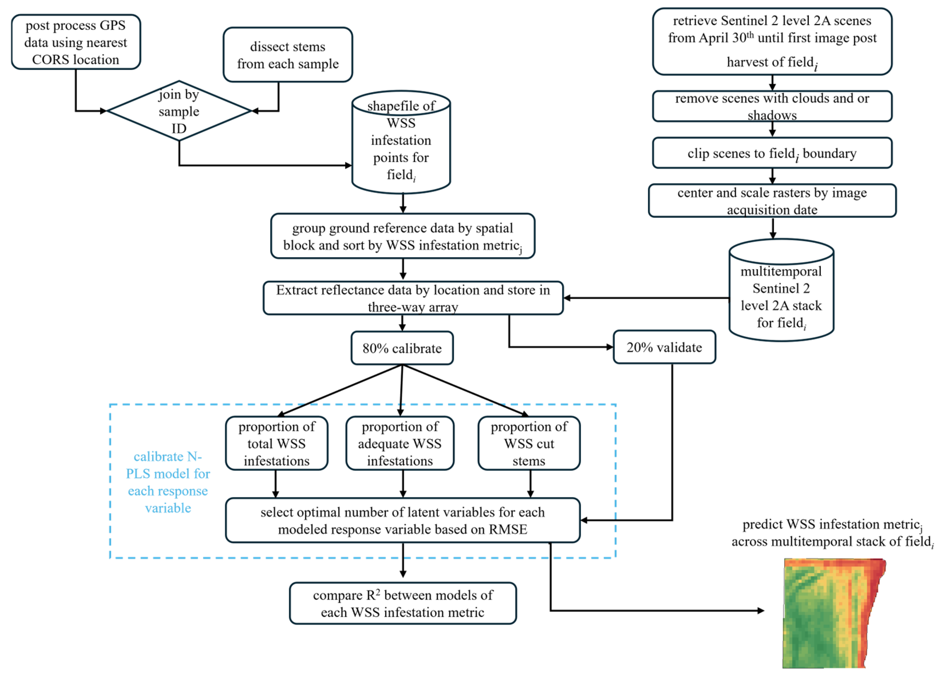
2. Materials and Methods

2.1. Site Selection and Ground Reference Data Collection

We selected wheat fields near Three Forks, Moccasin, Carter, and Big Sandy to capture environmental variation experienced in major wheat-producing regions (Figure 1). Both spring and winter wheat fields were selected in areas where producers had knowledge of damaging WSS populations. To quantify WSS infestation throughout a given field, we collected samples from discrete locations across each field. Sampling blocks were placed on the field edges adjacent to the nearest neighboring WSS source and non-source fields with transects leading inwards (Figure 2). In larger fields, additional sampling blocks were placed throughout the interior to account for variation in crop conditions. The distance between sampling locations along a transect was closest near the field edge and further apart as the transect moved inwards. The high density of sampling locations close to field edges was informed by previous studies [53,54,55] that found that WSS infestation severity and variation were greatest at the field edge and dissipated towards the interior. This general sampling scheme does not apply to Big Sandy 2020 as it was sampled before defining the aforementioned sampling criteria. In Big Sandy 2020, a small subset of infestation samples (n = 45) was collected before harvest from a small area to avoid trampling a large area of the growing crop. After harvest, a larger set was collected from the opposite side of the field (n = 100). Each wheat sample consisted of all the stems within 30 cm of a row and its corresponding location was recorded with an RS2 GNSS receiver (Emlid Reach, Richfield, OH). The GPS data for the sample locations were post-processed using temporally matched continuous operating reference station (CORS) data from the nearest CORS to each site in Emlid Studio (version 1.8). On average, the root mean square error (RMSE) of the corrected locations was less than a meter, well within the spatial resolution of the Sentinel 2 data (10–60 m).

The stem samples were then manually dissected to quantify the proportion of WSS infestation at each sample location. Leaves were removed from each stem prior to dissection to ensure signs of WSS infestation would not be obscured by desiccated leaf material. Using a scalpel, the length of each stem was dissected to record the presence of WSS frass, larvae, and parasitized WSS larvae. For stems that were infested by WSS, the number of stem nodes that larvae had burrowed through was also recorded. Stems were categorized in one of the following four categories: uninfested, dead neonate (WSS larvae that died before burrowing through a node), WSS burrowed through at least one node, or WSS cut. The most intensive feeding injury is represented by WSS cut as stems in this category have multiple nodes burrowed through and a complete severance at the base of the stem. Quantifying these proportional infestation metrics (p) at the sample level in this manner allowed us to represent and model WSS infestation in multiple ways, the most rudimentary of which is total WSS infestations, $p_{ total WSS}$, represented as the proportion of stems within a sample (i) that contained any evidence of WSS infestation (Equation (1)).

$${p_{ total WSS}}_i={\displaystyle \frac{{dead neonates}_i+{WSS burrowed through at least one node}_i+{WSS cut}_i}{{total stems}_i}}$$

(1)

We removed dead neonates to model WSS infestation as the proportion of instances where a larval WSS burrowed through at least one node or ultimately cut the stem (WSS cut), $p_{ adequate WSS}$ (Equation (2)).

$${p_{ adequate WSS}}_i={\displaystyle \frac{ {WSS burrowed through at least one node}_i+{WSS cut}_i}{{total stems}_i}}$$

(2)

Finally, we modeled WSS infestation as only the proportion of WSS cut stems within a sample, $p_{ WSS cut}$(Equation (3)).

$${p_{ WSS cut}}_i={\displaystyle \frac{ {WSS cut}_i}{{total stems}_i}}$$

(3)

To estimate how these metrics of WSS infestation vary within each field, we fit a generalized linear mixed model (glmm) using R (version 3.0.0) and the package ‘glmmTMB’ [58] for each field, followed by a post hoc comparison of means using the Tukey HSD method from the package ‘emmeans’ [59]. Because the WSS infestation metrics $p_{ total WSS}$, $p_{ adequate WSS}$, and $p_{ WSS cut}$ are measured as proportions of the total number of stems, which is binomial, we transformed the values with a logit link function. We incorporated a small adjustment factor that was added to observations of 0 and subtracted from values of 1 to avoid undefined logit values (Equation (4)). We also incorporated sample ID as a random effect to account for the fact that measurements of each WSS infestation metric were recorded at each location.

$$y_i=logit\left(p_i\right)=\mathit{ln}({\displaystyle \frac{p_i\pm 0.01}{1-(p_i\pm 0.01)}})$$

(4)

2.2. Sentinel 2 Imagery Acquisition and Time Standardization

Sentinel 2 surface reflectance scenes from across the growing season (1 April–first available image after field’s harvest date) were retrieved for each field using Google Earth Engine [60]. Because we were studying fields from 2020 to 2023, we used the harmonized Sentinel 2 surface reflectance Level 2A repository, as this collection shifts the range of a scene’s digital numbers post 25 January 2022 to match those before it [61]. We then manually removed scenes that contained clouds and/or shadows over the field of interest and clipped the remaining scenes to the field boundary to create a stack of images for each field. To standardize the image acquisition dates of each field and account for differences in locations, years, and crop type, we converted the date to growing degree days (GDDs) (see Equation (5) and Figure A1).

$$GDD=\left\{\begin{array}{c}{\sum }_{i=1}^n\max \left(T_{avg,i}-T_{base}\right) if spring wheat and i \ge P+7 \\ {\sum }_{j=1}^m\max \left(T_{avg,j}-T_{base}\right) if winter wheat and j\ge April 1 \end{array}\right.$$

(5)

where i represents days for spring wheat fields and j represents days for winter wheat fields. The model only considers days with an average temperature T_avg above T_base = 0 °C [62] starting seven days after the planting date (p) of spring wheat and starting on 1 April for winter wheat fields, as we did not have complete records of winter wheat seeding dates. Daily temperature data used for this were collected from PRISM https://prism.oregonstate.edu/ (accessed on 30 August 2024) [63]. For each field, the images were grouped by their values of GDDs, and the reflectance was centered and scaled to set each band mean equal to 0 and standard deviation to 1, and then stored in a three-way array [64,65]. Centering and scaling were applied in this manner to preserve variation in reflectance across GDDs but avoid bands with inherently greater magnitudes receiving more weight than those with lesser magnitudes in the modeling process [66].

2.3. Sampled WSS Infestation and Available Sentinel 2 Imagery

Fields sown to winter wheat represented the majority of those sampled in this study (six winter wheat, three spring wheat,

Table 1. Description of field locations, crop type, precipitation during the growing season (15 April–31 July), number of stem samples collected, cloud-free Sentinel 2 images available, planting, and harvest dates.

Field Name	Longitude	Latitude	Crop	Summer Precipitation (mm) a	No. of Wheat Samples	No. of Cloud-Free Images b	Planting Date	Harvest Date
Big Sandy 2020	110°21′41.76″W	48°16′9.84″N	Spring Wheat	165.0	145	10	28 April 2020	23 August 2020
Big Sandy 2022	110°23′39.84″W	48°16′3.72″N	Spring Wheat	117.3	115	10	11 April 2022	13 August 2022
Carter 2023	110°57′51.12″W	47°45′35.28″N	Winter Wheat	221.6	98	8	N/A	26 July 2023
Moccasin 2021 A	109°52′39.72″W	47°5′47.40″N	Winter Wheat	135.2	100	15	N/A	30 July 2021
Moccasin 2021 B	109°51′33.84″W	47°4′5.88″N	Winter Wheat	135.2	90	17	27 September 2021	30 July 2021
Moccasin 2022	109°52′3.36″W	47°4′2.64″N	Winter Wheat	179.9	139	16	N/A	4 August 2022
Moccasin 2023	109°51′33.84″W	47°4′5.88″N	Winter Wheat	297.5	100	16	N/A	8 August 2023
Three Forks 2022	111°36′7.20″W	46°0′57.96″N	Spring Wheat	177.5	225	12	5 April 2022	20 August2022
Three Forks 2023	111°35′38.04″W	45°59′22.20″N	Winter Wheat	178.3	146	13	15 September 2023	21 August 2023

^a, PRISM Climate Group [63]; ^b, Google Earth Engine [60].

). The fields received between 117.3 and 297.5 mm of rainfall during the growing season, as estimated from PRISM https://prism.oregonstate.edu/ (accessed on 30 August 2024) [63]. In total, we collected 1158 ground reference samples, from which we manually dissected 43,155 wheat stems to measure WSS infestation. The number of Sentinel 2 images suitable for analysis varied due to cloud cover during the satellite revisits and location in relation to the constellation’s orbit. For instance, the Moccasin area benefited from a greater number of available images, as the area is resampled by a Sentinel 2 satellite every second or third day, whereas the other fields studied are revisited every fifth day. After removing images containing clouds and/or shadows, fields had between 8 and 17 images suitable for further analysis. Although we were not able to collect all sowing dates, records of harvest dates were complete.

2.4. Sparse Multiway Partial Least Squares Regression Models

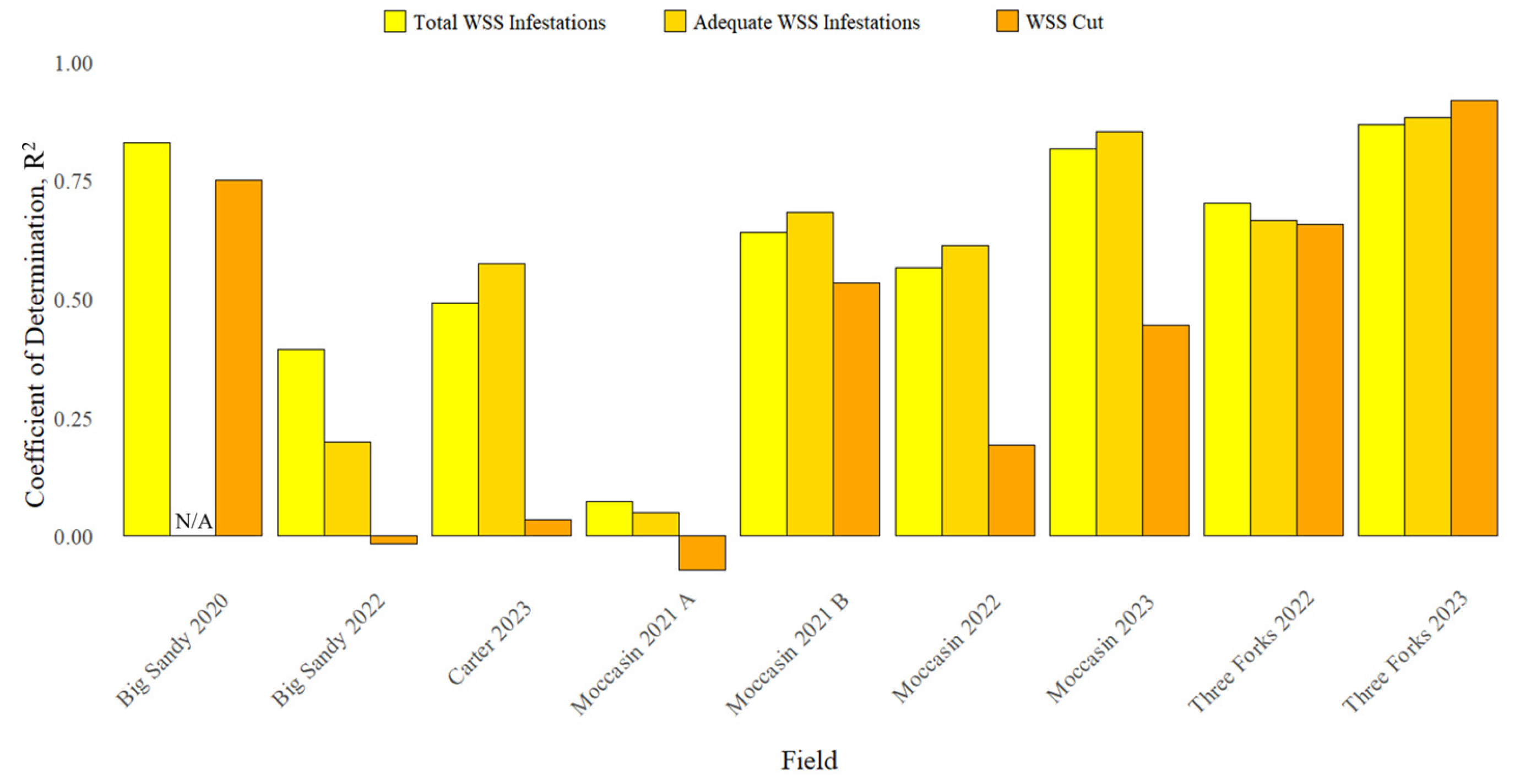
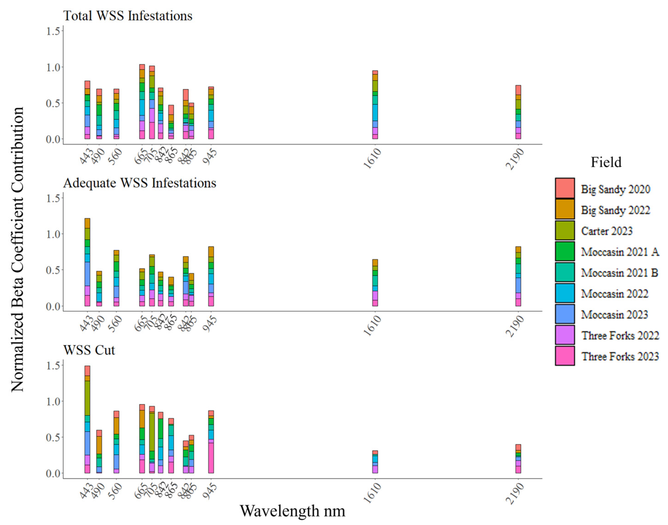
To investigate our research objective, of which the metric of WSS infestation is most accurately estimated with multitemporal satellite imagery, we produced a model for each field for each of our three response variables: total WSS, adequate WSS, and WSS cut. The Big Sandy 2020 field did not have stem dissection data that accounted for adequate WSS; thus, we only produced models of total WSS and WSS cut for that field. Centering and scaling were then applied to the logit values for each metric from each field to amend overdispersion and improve overall model performance.

For each field, the data were then partitioned into a model calibration and validation set based on spatial blocking and WSS infestation level. Spatial blocking was used to account for the spatial dependence of observations [67] and stratifying by infestation level to account for the non-normal distributions of each WSS infestation metric. For each spatial block, the data were sorted in descending order based on the metric of WSS infestation for a given model, and every fifth observation was placed into a validation set while the remaining 80% of the data were used to calibrate the model. Model residuals were plotted against each point’s distance from the field edge to verify that there were no issues with assumption of independence of observations due to the nature of the WSS infestation patterns (Supplementary Figures S1–S3).

R (version 3.0.0) [68] was used to fit sparse N-PLS models for each WSS infestation metric from each field using the package ‘sNPLS’ [69]. The sNPLS function preforms trilinear decomposition on the three-way array of images and the response vector of the WSS infestation metric to explain the maximum amount of covariance between both elements [64,65]. Concurrent with this process, Hervás et al. (2019) [70] implemented feature selection with the least absolute shrinkage and selection operator (LASSO) [71] to select a subset of spectral measurements from the three-way array of images that is most important in explaining the variation in the chosen WSS infestation metric. The relationship between the selected spectral measurements and the WSS infestation metric is modeled by a set of orthogonal factors referred to as latent variables [64]. Model selection is performed by conducting a grid search across all possible combinations of Sentinel 2 bands, available images, and number of latent variables by evaluating the RMSE between the calibration and validation set [72] (

Table A1. Model parameters and performance metrics for the optimal sparse multi-way partial least squares regression model produced for total WSS infestations for a given field. The normalized root mean square error (RRMSE) calculated by dividing the RMSE of each dataset by its mean to provide comparative power across all models.

Field	No. Latent Variables	No. Time-Points	No. Bands	Calibration RRMSE	Validation RRMSE	Calibration r2	Validation r2	Calibration R2	Validation R2
Big Sandy 2020	10	9	5	0.528	0.438	0.835	0.921	0.698	0.830
Big Sandy 2022	8	9	11	0.557	0.626	0.606	0.663	0.353	0.393
Carter 2023	7	7	3	0.318	0.358	0.788	0.759	0.612	0.491
Moccasin 2021A	9	1	11	0.647	5.039	0.948	0.513	0.894	0.073
Moccasin 2021B	7	1	10	0.528	0.754	0.854	0.859	0.720	0.641
Moccasin 2022	5	1	2	0.884	0.924	0.648	0.791	0.375	0.567
Moccasin 2023	9	1	9	0.396	0.323	0.874	0.911	0.759	0.816
Three Forks 2022	2	1	7	0.338	0.309	0.893	0.874	0.753	0.702
Three Forks 2023	10	1	3	0.757	0.935	0.942	0.942	0.885	0.869

,

Table A2. Model parameters and performance metrics for the optimal sparse multi-way partial least squares regression model produced for adequate WSS infestations for a given field. The normalized root mean square error (RRMSE) calculated by dividing the RMSE of each dataset by its mean to provide comparative power across all models.

Field	No. Latent Variables	No. Time-Points	No. Bands	Calibration RRMSE	Validation RRMSE	Calibration r2	Validation r2	Calibration R2	Validation R2
Big Sandy 2020	* N/A
Big Sandy 2022	10	4	12	0.598	0.818	0.587	0.488	0.297	0.199
Carter 2023	10	1	5	0.379	0.352	0.725	0.817	0.513	0.574
Moccasin 2021A	10	11	11	0.626	4.51	0.951	0.404	0.891	0.049
Moccasin 2021B	2	1	11	0.577	0.689	0.819	0.873	0.668	0.682
Moccasin 2022	6	16	11	0.969	1.015	0.666	0.799	0.392	0.612
Moccasin 2023	6	1	1	0.422	0.301	0.866	0.938	0.739	0.854
Three Forks 2022	2	4	8	0.395	0.413	0.877	0.823	0.744	0.665
Three Forks 2023	10	4	11	0.856	0.810	0.922	0.941	0.848	0.882

* Information for adequate WSS infestations was not collected for Big Sandy 2020.

and

Table A3. Model parameters and performance metrics for the optimal sparse multi-way partial least squares regression model produced for WSS cut for a given field. The normalized root mean square error (RRMSE) calculated by dividing the RMSE of each dataset by its mean to provide comparative power across all models.

Field	No. Latent Variables	No. Time-points	No. Bands	Calibration RRMSE	Validation RRMSE	Calibration r2	Validation r2	Calibration R2	Validation R2
Big Sandy 2020	7	10	11	0.905	0.682	0.709	0.868	0.428	0.752
Big Sandy 2022	10	9	1	0.816	2.275	0.515	0.426	0.219	−0.016
Carter 2023	1	3	2	0.783	1.001	0.358	0.421	0.087	0.035
Moccasin 2021A	9	4	2	0.851	9.25	0.872	0.216	0.705	−0.072
Moccasin 2021B	10	11	1	0.936	0.984	0.728	0.757	0.489	0.534
Moccasin 2022	7	4	1	0.913	1.568	0.715	0.49	0.427	0.191
Moccasin 2023	9	12	7	0.507	0.994	0.874	0.735	0.756	0.444
Three Forks 2022	2	4	8	0.574	0.528	0.762	0.814	0.566	0.657
Three Forks 2023	10	7	1	1.144	0.788	0.877	0.965	0.749	0.918

).

To determine which WSS infestation metric is most accurately estimated using multitemporal RS, we compared the coefficient of determination from the validation datasets across all models. We chose R² as the metric to judge model performance as it is a dimensionless value that subtracts the ratio of the residual sum of squares and total sum of squares from one, to represent how well a model fits a given dataset (Equation (6)). In this context, R² is bound between negative infinity and one, where an R² value of one indicates that the model perfectly fits the data and zero or less indicates a poor fit. A one-way repeated measures ANOVA, followed by a post hoc Tukey HSD test, was conducted using the ‘lme4’ [73] and ‘emmeans’ [59] packages to assess whether R² varied by WSS infestation metric, while accounting for the study’s repeated measures design. The Big Sandy 2020 field was removed from this analysis, as we did not have information for adequate WSS infestations. Model diagnostics revealed no issues with normality, residuals, or homoscedasticity. The methods presented in this section are summarized in Figure 3.

$${\mathrm{R}}^2=1-{\displaystyle \frac{\sum _{i=1}^n{(y_i-{\hat{y}}_i)}^2}{\sum _{i=1}^n{(y_i-\overline{y})}^2 }}$$

(6)

3. Results

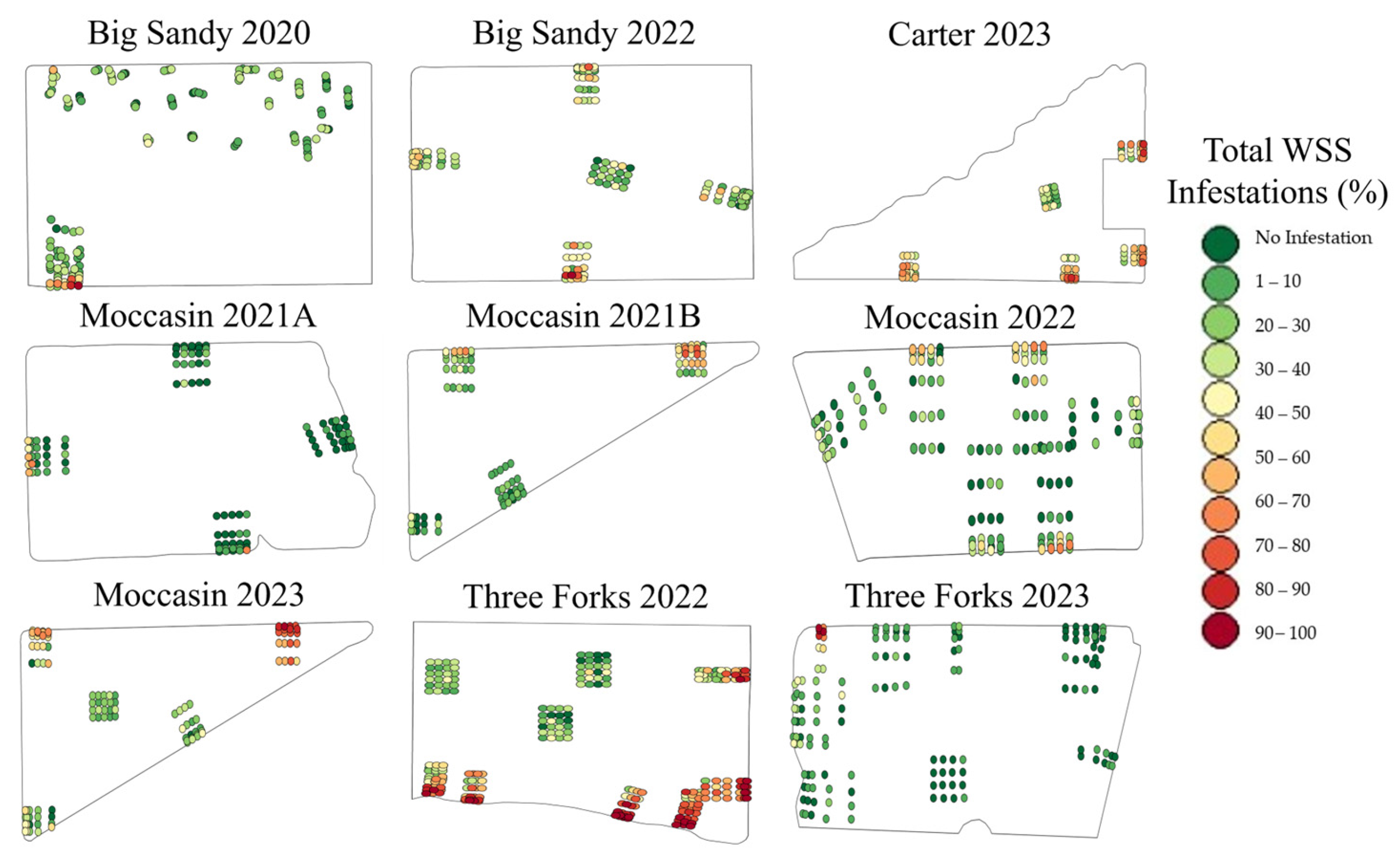
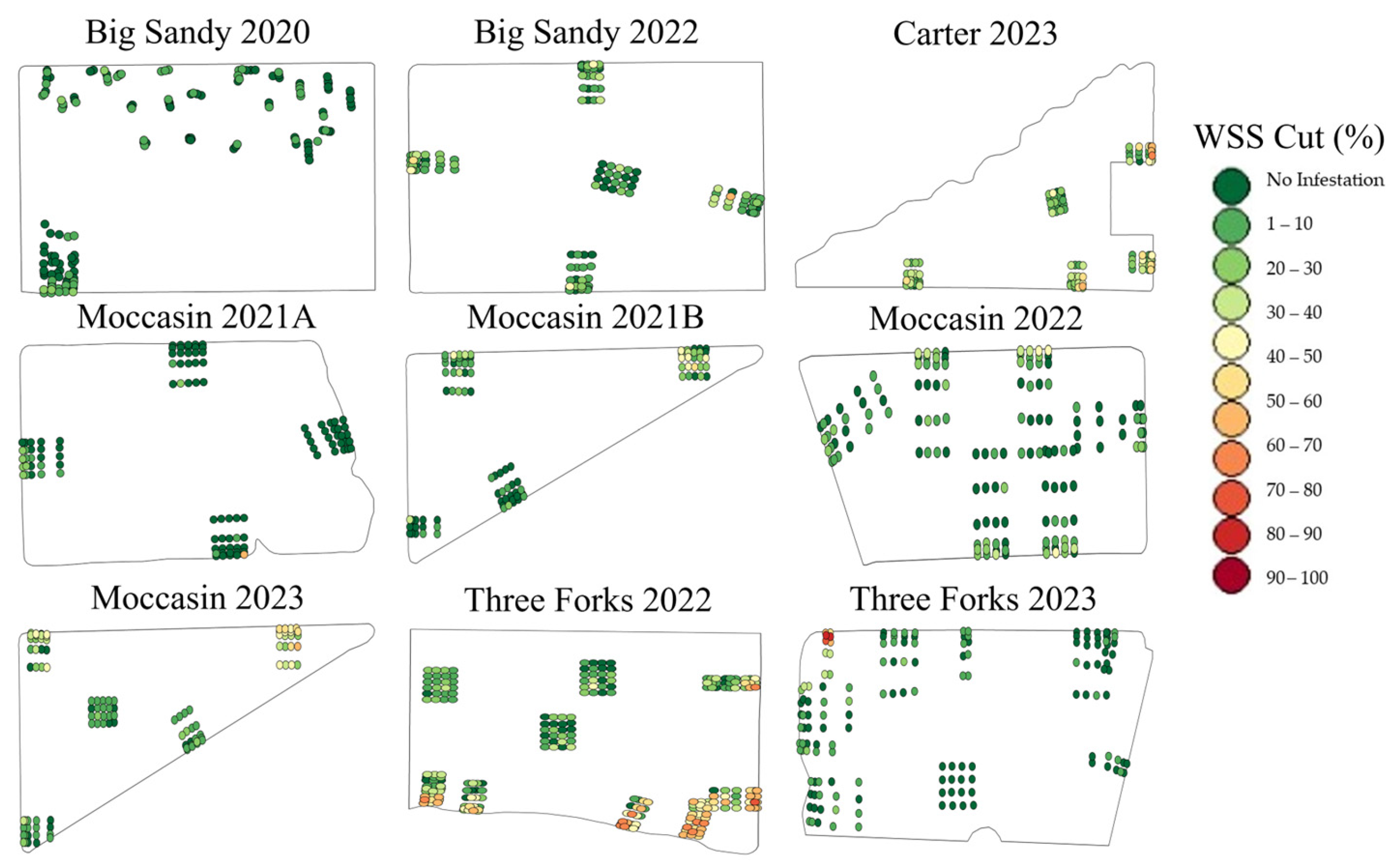
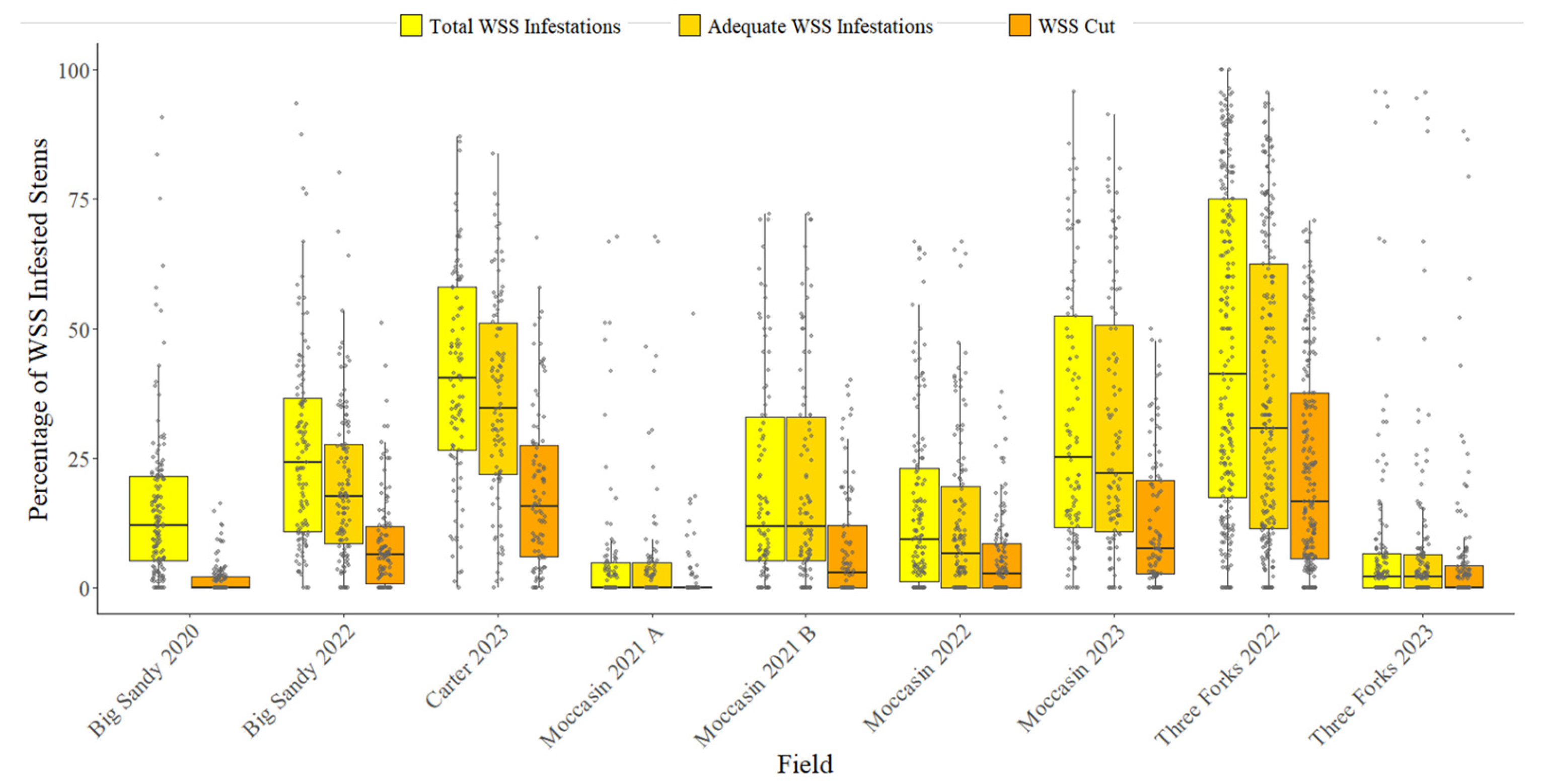
3.1. Surveyed WSS Infestation

Sampled WSS infestation varied across fields with a range of 5.9–45.67% total WSS infestation. The mean total WSS infestation across all sampled fields was 24.7% with a mean adequate WSS percentage of 22.3% and a mean WSS cut percentage of 10.3% (Figure 4). On average, total WSS infestation was 2.5 times greater than the percentage of WSS cut; similarly, the percentage of adequate WSS-infested stems was 2.2 times greater than WSS cut (excluding Big Sandy 2020 for not having adequately WSS-infested stems). WSS infestation varied spatially throughout fields (Figure A2, Figure A3 and Figure A4), and many samples had little to no infestation, which led to high variance and overdispersion in the datasets (

Table 2. Mean and standard deviation for the observed proportion of total wheat stem sawfly (WSS) infestations, adequate WSS infestations, and WSS cut for each sampled field. Each field was fit to a generalized linear mixed model to account for the proportional nature of the response using a logit link function and a random effect for the repeated measures from sample location. Letters next to the mean indicate significant differences (p-value < 0.05) among WSS infestation metrics within each field, as indicated by a post hoc comparison of means adjusted using the Tukey honest significant difference method.

Field	Total WSS Infestations	Adequate WSS Infestations	WSS Cut
Big Sandy 2020	15.64 A ± 15.68	N/A	1.51 B ± 2.97
Big Sandy 2022	26.78 A ± 18.98	20.13 B ± 15.20	8.59 C ± 9.59
Carter 2023	40.75 A ± 20.52	36.43 B ± 19.58	18.8 C ± 15.46
Moccasin 2021 A	5.92 A ± 13.56	5.48 A ± 12.66	1.75 B ± 6.26
Moccasin 2021 B	20.35 A ± 20.40	20.24 A ± 20.39	7.76 B ± 10.88
Moccasin 2022	15.18 A ± 17.29	12.31 B ± 15.60	5.57 C ± 7.89
Moccasin 2023	32.42 A ± 25.36	31.26 A ± 25.0	12.79 B ± 13.13
Three Forks 2022	45.67 A ± 31.01	36.90 B ± 28.80	22.92 C ± 20.30
Three Forks 2023	8.18 A ± 18.12	7.89 A ± 17.65	5.72 B ± 14.57

). In all fields, total WSS was found to be significantly different than WSS cut, as indicated by a post hoc comparison of means using a Tukey HSD test (p-value < 0.05; Table 2). In four of the eight fields that had measurements of both total and adequate WSS infestations, these metrics were found to be statistically different.

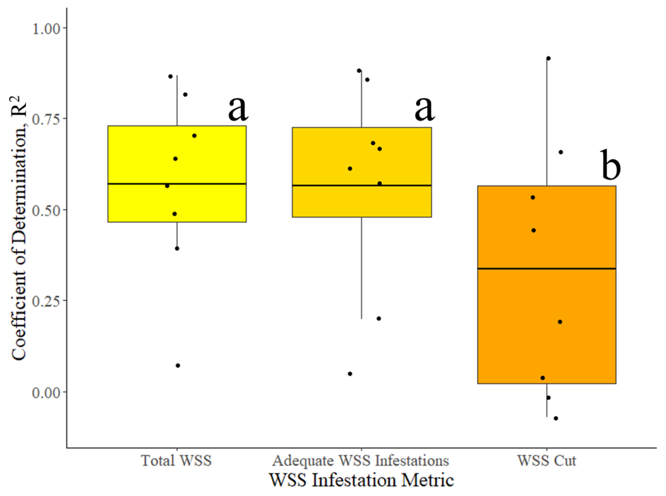
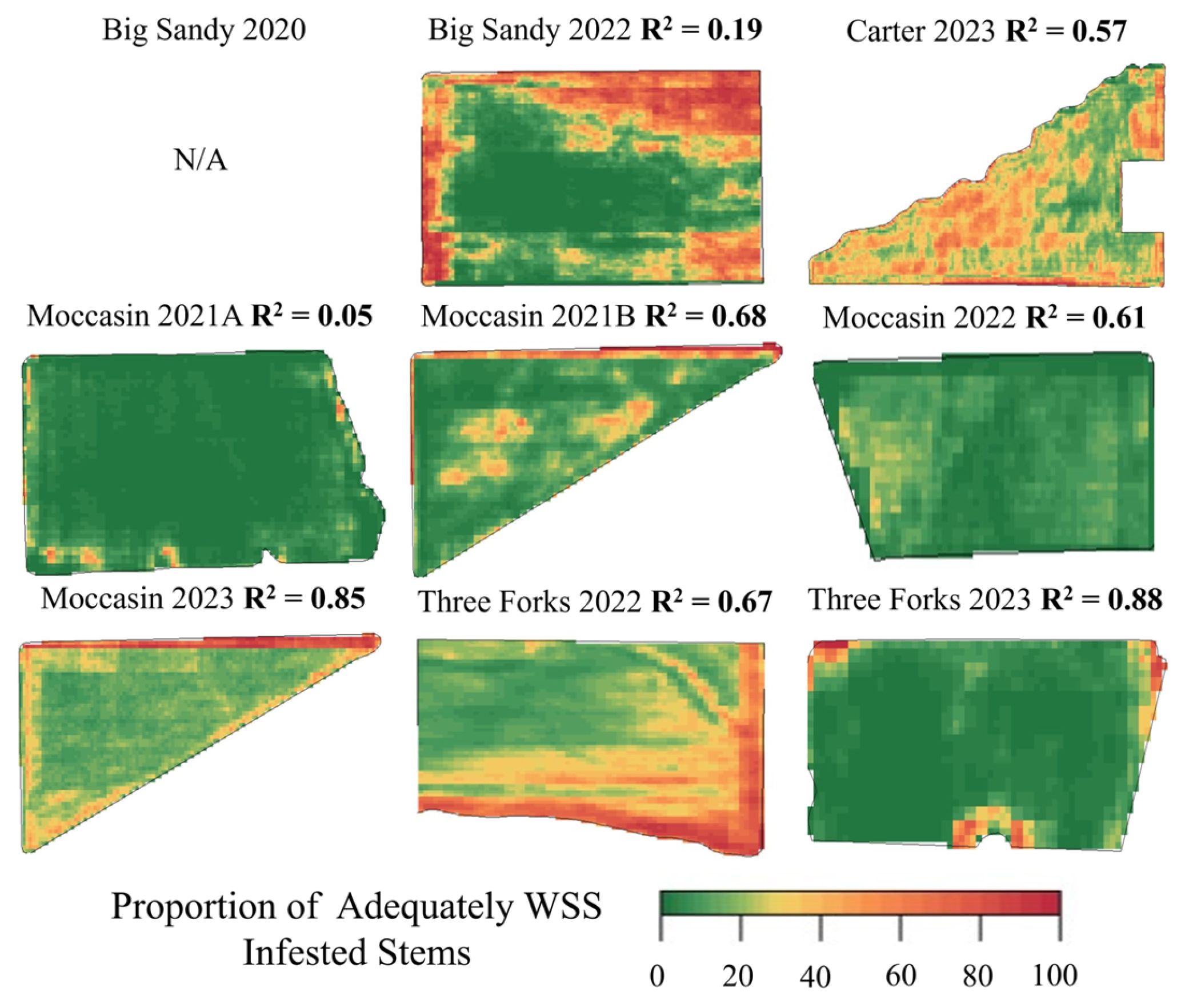
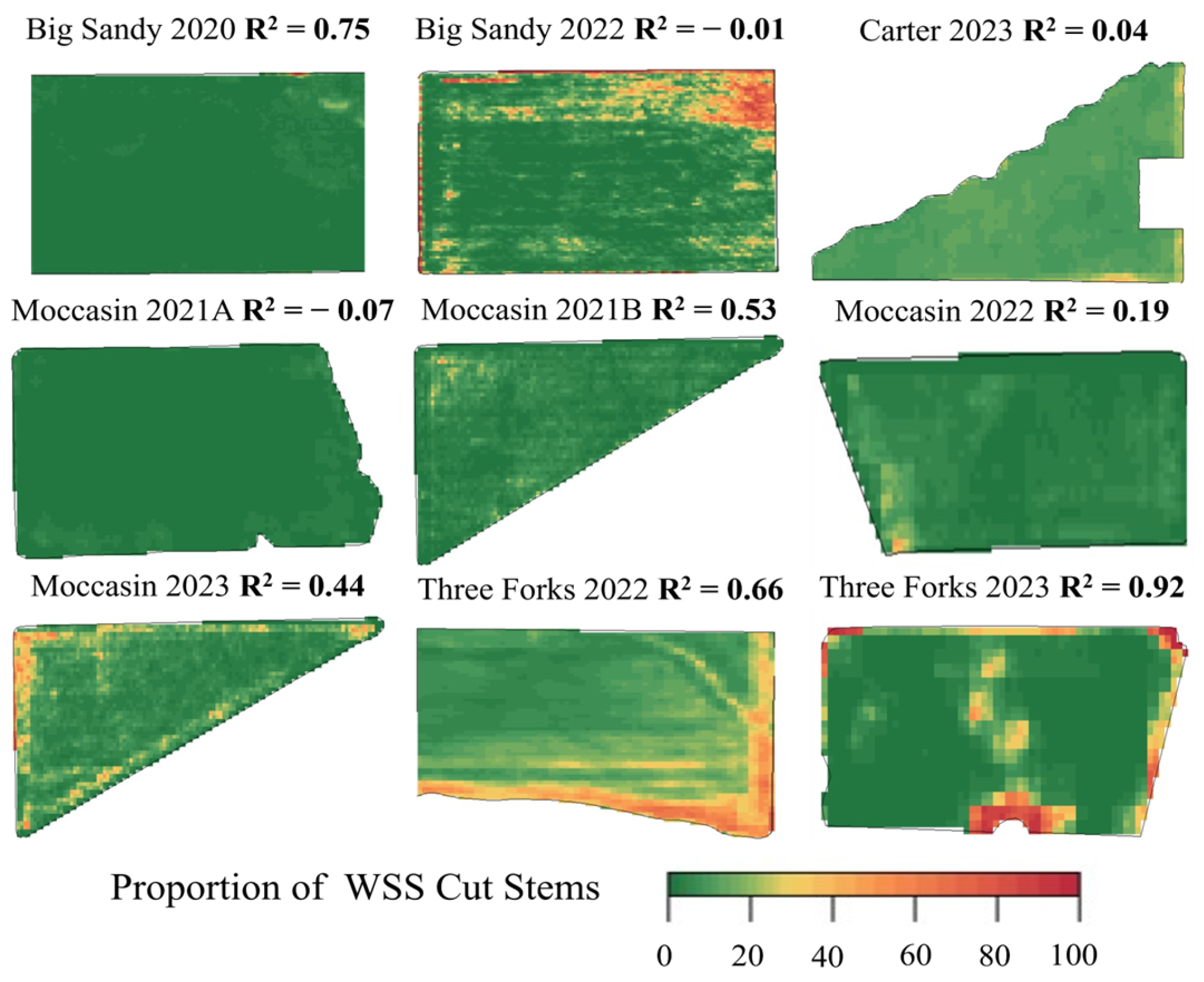
3.2. Modeled WSS Infestation

Model performance varied across fields and infestation metrics, as indicated by the R² value from the validation dataset of the optimal model for each WSS infestation metric for a given field (Figure 5). The average R² was greatest for total WSS (mean = 0.57, standard deviation (SD) = 0.26), and adequate WSS (mean = 0.57, SD = 0.29), while WSS cut was, on average, markedly lower (mean = 0.25, SD = 0.35). Furthermore, the best fitting model for WSS cut of the fields Big Sandy 2022 and Moccasin 2021 A had negative values of R², indicating that the models produced a larger residual sum of squares than the total sum of squares, resulting in a very poor fit to the validation data.

We found strong evidence to suggest that R² varied across models of WSS infestation metrics while accounting for the random effect of field (χ² = 19.38, df = 2, p < 0.001; Figure 6). The mean R² for total and adequate WSS infestation was almost identical at 0.57 (SD = 0.26) and 0.57 (SD = 0.30), respectively. In contrast, the mean R² for WSS cut was 0.34 (SD = 0.36). Following this up with pairwise comparisons using Tukey’s method showed that the total WSS infestation group was significantly different from the WSS cut group, with an estimated mean difference of 0.23 (df = 14, t-ratio = 3.85, p-value = 0.005). Similarly, the adequate WSS group was significantly different from WSS cut, with an estimated mean difference of 0.23 (df = 14, t-ratio = 3.77 p-value = 0.005). However, the difference between total WSS and adequate WSS was not statistically significant (df = 14, t-ratio = 0.07, p-value = 0.997). This indicates that while WSS cut is distinct from the other groups, total WSS and adequate WSS are not significantly different from each other.

The mapped predictions of each WSS infestation metric display the expected pattern of clusters of high infestation near field edges with severity of infestation decreasing towards field interiors (Figure 7, Figure 8 and Figure 9). The trend of high WSS infestation along field edges is most clearly illustrated in the total WSS maps for fields Moccasin 2021B, Big Sandy 2022, Three Forks 2022, Carter 2023, and Moccasin 2023 (Figure 7). Coincidentally, these were also the fields with the highest observed WSS infestation (Table 1). The maps generally mirror the trend in the sampled WSS infestation metric they are derived from, as WSS cut is predicted minimally across the fields (Figure 9), while the adequate WSS maps estimate infestation events to a greater extent than WSS cut, but to a lesser degree than total WSS. The WSS cut maps primarily confine predictions of cutting to the edges of the fields, whereas the maps for adequate and total WSS indicate non-zero values for their respective metrics in areas beyond the field edges to a greater extent.

Images from the later stages of the growing season were weighted with the greatest importance across all modeled WSS infestation metrics (Figure 10). This was determined by extracting the magnitude of the beta coefficients, which directly represent the importance of explanatory variables in N-PLS [74], and normalizing the absolute values by dividing them by the sum of the absolute beta coefficients for a given model. To understand how beta coefficients are distributed across crop and WSS phenology, we plotted the normalized beta coefficients against quantiles of GDDs. This was conducted by computing four quantiles for the GDD distribution of each field to remedy the variance in GDD ranges observed across all fields. Across models of all WSS infestation metrics, Sentinel 2 images from the last quantile were ascribed the most weight, indicating that images closer to the date of harvest are vital to estimating WSS infestation.

In visualizing the relationship between these normalized beta coefficients and their distribution across the wavelengths measured by Sentinel 2 (Figure 11), it appears that all bands are useful in explaining variability in WSS infestations. The shortwave infrared (SWIR) bands centered at 1610 and 2190 nm appear to have more utility to models predicting total or adequate WSS infestation than models of WSS cut.

4. Discussion

The methods used in this study most accurately estimated the metrics of total and adequate WSS infestation as compared to the proportion of cut stems (Figure 6). Models of cut stems had the greatest variance, and this was the only metric to produce models with negative values of R² (Figure 5 and Figure 6). These results provide evidence that multitemporal passive RS for estimating the post-harvest level of WSS infestation benefits from complete dissections of available stems and images with bands distributed across the VSWIR.

The studied fields are representative of the diverse areas of wheat production found across Montana, and with it, variation in environment, agronomic practices, and WSS populations. We sought to remedy the discrepancies between fields, years, cultivars, and availability of cloud-free Sentinel 2 images by calibrating and validating each model within the context of a given field. To standardize the temporal domain across the crop and WSS phenology of field years, we used a GDD model with starting parameters specific to spring or winter wheat [62] (Equation (5), Figure A1). Furthermore, we took into account spatial variability and possible effects of lurking variables (heterogeneity of soil conditions, weeds, other insect damage) that we were not able to measure in this study, with the following precautions: (1) partitioning calibration and validation data sets to have proportional levels of infestation equally distributed across the sampling blocks of the field, (2) centering and scaling each field’s available Sentinel 2 images by band and GDD, and (3) using a multiway model (sparse N-PLS) to estimate WSS infestation based on the spectral trajectory of the observations while accounting for the correlative nature of the reflectance measurements across the spectral and temporal domains. Despite variation in locations, years, cultivars, agronomic conditions, or available imagery, the results of this study indicate that the methods we used for multitemporal passive RS are better suited for estimating total or adequately WSS-infested stems as opposed to cut stems.

We found that average R² was similar for total and adequately WSS infestation models, but models of WSS cut had a significantly lower R² while accounting for the random effect of field (Figure 6). This indicates that regardless of spring or winter wheat, location, or variation between years, these methods were least consistent for estimating the proportion of WSS cut stems. Interestingly, the highest R² of any model was reported for the proportion of cut stems in the field Three Forks 2023 (R² = 0.92). Then again, the only models with negative values of R² were also created for the metric cut stems (Moccasin 2021 A, R² = −0.07 and Big Sandy 2022, R² = −0.01; Figure 9). It is worth noting that the fields Moccasin 2021 A and Big Sandy 2022 produced the lowest performing models for all metrics across all fields studied. We do know that Big Sandy 2022 received the least amount of summer rainfall (Table 1) of any field studied, and the producer noted that there was a damaging hail event (unpublished data). It is possible that the influences of prolonged water stress and a hailstorm could mask or confound variation in spectral reflectance related to the distribution of WSS infestation. Moccasin 2021 A did not seem to be subjected to drought or hail but did record the lowest sampled levels of both total and adequate WSS infestation, both of which were over-dispersed (Table 2). To ameliorate the effects of overdispersion on model performance, we used centering, scaling, and partitioning of the data to balance the proportions of infestation in the calibration and validation sets [75].

It is possible that the small number of observations with measurable infestation create high enough leverage on the model to produce poor validation results (Table A1, Table A2 and Table A3). Despite this, the field Three Forks 2023 had similar issues with low levels of infestation and overdispersion across all WSS infestation metrics (Table 2) but reported high R² values for all WSS infestation metrics. As previously noted, one of the limitations of this study is the absence of possible lurking variables, which makes it difficult to interpret why some models explained more variation in WSS infestation than others. This suggests that future studies should incorporate in situ measurements of other important abiotic and biotic factors that could impact crop performance and reflectance. Integrating variation in important environmental parameters with WSS infestation surveys could help produce models that better estimate WSS infestation within fields. Moreover, this variation in model performance across field years indicates that georegistered stem dissection surveys are necessary for creating these models.

Across the best performing models of each WSS infestation metric, the last quantile of GDDs was attributed with the greatest relative contribution of beta coefficients (Figure 10). This suggests that RS images from the end of the growing season are particularly important in explaining variation across all WSS infestation metrics. Since our modelling approach enforced sparsity by only selecting covariates (i.e., reflectance of individual bands given the GDD) that significantly explained variation in the dependent variable (based on the WSS infestation metric) [70], and most models incorporated data from more than two GDD quantiles, it can be implied that partial explanatory power is afforded by images from multiple points in the growing season. Moreover, this dispersed pattern of beta coefficients varying by both field and infestation metric is also present across the distribution of Sentinel 2 bands (Figure 11). While model performance varies across fields and WSS infestation metrics, all models benefited from images collected across the entire growing season with Sentinel 2’s coverage of the VSWIR.

The models in this paper behaved similarly to a model presented by Ermatinger et al. (2024) [44] trained for proximal estimation of adequate WSS infestations in wheat via multitemporal hyperspectral measurements. Ermatinger et al. (2024) [44] found that SWIR radiation was important for predicting the proportion of adequately WSS-infested stems, a finding that is consistent with the importance of the Sentinel 2 SWIR bands centered at 1620 and 2190 nm in Figure 11. Because the water content of crops like wheat influences SWIR absorbance and reflectance [46], the importance of SWIR radiation for explaining variation in WSS infestation metrics may be a result of early season variation in crop condition related to WSS oviposition patterns [56], or WSS larval feeding injury that decreases water content later in the season [49,50]. In both studies, spectral data throughout the VSWIR over the entire course of the WSS host interaction were important, but the greatest emphasis was placed on spectral measurements near host senescence. It is logical to assume this is because the compounding effects of WSS feeding manifest in spectral changes that are most discernable at the end of the growing season, especially increased SWIR reflectance related to impaired stem water transport from larval WSS feeding on vascular bundles [38]. If this were the case, we may expect that images from the last GDD quantile would have greater importance for models of the most invasive forms of WSS infestation metric: WSS cut or adequate, as opposed to total WSS infestation. However, the reason for the shared importance of the last GDD quantile across all metrics may be explained by the hierarchal nature of the measured WSS infestation metrics (i.e., total WSS infestation ≥ adequate WSS infestations ≥ WSS cut; Table 2 and Figure 4). In other words, the areas with the greatest degree of cutting will invariably have an equal or greater degree of adequate and total infestation (Figure A2, Figure A3 and Figure A4). Therefore, in the case of this study, covariates found to explain variation in WSS cutting will also lend explanatory power to the metrics total and adequate WSS infestation. This nested relationship of the WSS infestation metrics also provides an explanation as to why early-season reflectance measurements have value for estimating all metrics of WSS infestation. From an ecological perspective, early-season variation in crop condition across a field may influence where female WSS congregate and, in turn, lay their eggs [56,76,77,78]. Thus, it is empirically true that the areas of greatest total WSS infestation have greater potential for WSS cutting than areas with a lesser degree of total WSS infestation. However, factors like pith expression, fungal infection, and parasitism influence a WSS larvae’s ability to survive the growing season and cut the stem [39], which may partially explain why the model R² of WSS cut had the greatest variance and the lowest mean (Figure 6). The comparison of average model performance for each metric demonstrates that multitemporal passive RS of WSS is least compatible with estimating the degree of WSS cutting.

Maps of total or adequate WSS infestation describe dispersal and oviposition patterns of WSS, but these metrics alone do not capture the impact of management techniques on WSS. Precise estimates of cutting, combined with total WSS infestation at the end of the growing season, would offer the most robust insights into how management techniques impact WSS and could help forecast next year’s WSS pressure. End-of-season cutting estimates are likely most useful to wheat producers because a lack of viable in-season management options for WSS means decisions need to be made prior to planting. WSS management decisions often involve modifications to planting date, solid-stem varieties, or crop rotation [4]. Although some models of cutting were satisfactory, the inconsistent performance among models of cutting illustrates that multitemporal passive RS is likely not sufficient for estimating WSS cutting. This would suggest that future studies should consider active methods of remote sensing like synthetic aperture radar (SAR) [79] or light detection and ranging (LiDAR) [80] sensors that are sensitive to structural variation, such as crop lodging from WSS cutting. Caution should be owed to the fact that rates of cutting are not always synonymous with the degree of lodging as falling stems can create a domino effect and lodge uncut stems. Moreover, low levels of cutting may not manifest in detectable lodging, or events like hailstorms can induce lodging in the absence of WSS infestations. Combining post-harvest stem dissection surveys with multitemporal passive RS and active RS concurrent with WSS cutting may present the most robust approach for estimating both total WSS infestation and cutting.

5. Conclusions

Damaging populations of WSS have existed for more than a century in North America and are currently expanding their geographic range. Despite a longstanding economic interest in the pest, producers of wheat have a limited number of management techniques at their disposal. This issue has been further compounded by an insufficient ability to monitor WSS populations at the field and regional scale. Due to the concealed lifecycle of WSS, accurate estimates of larval WSS infestation, mortality, and cutting rely on comprehensive stem dissection campaigns from the end of the growing season. The results of this study indicate that these surveys can be combined with multitemporal Sentinel 2 imagery to estimate the level of total (R² = 0.57) and adequate WSS infestations (R² = 0.57) more accurately than the level of WSS cutting (R² = 0.34). It is likely that RS-based models of cutting would benefit from the inclusion of SAR or LiDAR data. Future studies on RS of WSS are encouraged to co-locate stem dissection surveys with measurements of other environmental parameters that influence the reflectance of wheat, such as soil conditions, weed encroachment, and insect herbivory. Long-term monitoring of WSS pressure in the context of environmental variation and management tactics can help consolidate management techniques into a cohesive strategy to provide resiliency against WSS. This work demonstrates an important first step in using RS technologies to unveil the subtleties of WSS infestation at the field scale across variable growing regions and agronomic practices.

References

1. Beres, B.L.; Dosdall, L.M.; Weaver, D.K.; Cárcamo, H.A.; Spaner, D.M. Biology and Integrated Management of Wheat Stem Sawfly and the Need for Continuing Research. Can. Entomol. 2011, 143, 105–125. [Google Scholar] [CrossRef]
2. Criddle, N. The Western-Stem Sawfly and its Control. Dom. Can. Dept. Ag. 1922, 6, 1–8. [Google Scholar]
3. Weaver, D. Wheat Stem Sawfly (Cephus cinctus Norton). In Advances in Understanding Insect Pests Affecting Wheat and Other Cereals; Eigenbrode, S.D., Rashed, A., Eds.; Burleigh Dodds Science Publishing Limited: Cambridge, UK, 2023; pp. 93–134. [Google Scholar]
4. Weaver, D.; Tallman, S.; Lane, T. Wheat Stem Sawfly Best Management Practices; MSU Extension Bulletin EB0244; USDA-NRCS Agronomy Technical Note MT-95; Montana State University: Bozeman, MT, USA, 2024. [Google Scholar] [CrossRef]
5. Morrill, W.L.; Gabor, J.W.; Kushnak, G.D. Wheat Stem Sawfly (Hymenoptera: Cephidae): Damage and Detection. J. Econ. Entomol. 1992, 85, 2413–2417. [Google Scholar] [CrossRef]
6. Norton, E. Notes on North American Tenthredinidæ, with Descriptions of New Species. Trans. Amer. Entomol. Soc. (1867–1877) 1872, 4, 77–86. [Google Scholar] [CrossRef]
7. Criddle, N. The Life Habits of Cephus cinctus Norton in Manitoba. Can. Entomol. 1923, 55, 1–4. [Google Scholar] [CrossRef]
8. Fletcher, J. The Western Wheat Stem Sawfly (Cephus pygmaeus L.). Dom. Can. Dept. Ag. Rep. Dom. Entomol. 1896, 1, 147–149. [Google Scholar]
9. Ainslie, C.N. The Western Grass-Stem Sawfly a Pest of Small Grains. In U.S. Department of Agriculture Technology Bulletin; US Department of Agriculture: Washington, DC, USA, 1929; Volume 157, pp. 1–23. [Google Scholar]
10. Bekkerman, A.; Weaver, D.K. Modeling Joint Dependence of Managed Ecosystems Pests: The Case of the Wheat Stem Sawfly. J. Ag. Res. Econ. 2018, 43, 172–194. [Google Scholar]
11. Beres, B.L.; Cárcamo, H.A.; Byers, J.R. Effect of Wheat Stem Sawfly Damage on Yield and Quality of Selected Canadian Spring Wheat. J. Econ. Entomol. 2007, 100, 79–87. [Google Scholar] [CrossRef] [PubMed]
12. Cockrell, D.M.; Randolph, T.; Peirce, E.; Peairs, F.B. Survey of Wheat Stem Sawfly (Hymenoptera: Cephidae) Infesting Wheat in Eastern Colorado. J. Econ. Entomol. 2021, 114, 998–1004. [Google Scholar] [CrossRef]
13. Lesieur, V.; Martin, J.-F.; Weaver, D.K.; Hoelmer, K.A.; Smith, D.R.; Morrill, W.L.; Kadiri, N.; Peairs, F.B.; Cockrell, D.M.; Randolph, T.L.; et al. Phylogeography of the Wheat Stem Sawfly, Cephus cinctus Norton (Hymenoptera: Cephidae): Implications for Pest Management. PLoS ONE 2016, 11, e0168370. [Google Scholar] [CrossRef]
14. McCullough, C.T.; Hein, G.L.; Bradshaw, J.D. Phenology and Dispersal of the Wheat Stem Sawfly (Hymenoptera: Cephidae) into Winter Wheat Fields in Nebraska. J. Econ. Entomol. 2020, 113, 1831–1838. [Google Scholar] [CrossRef] [PubMed]
15. Olfert, O.; Weiss, R.M.; Catton, H.; Cárcamo, H.; Meers, S. Bioclimatic Assessment of Abiotic Factors Affecting Relative Abundance and Distribution of Wheat Stem Sawfly (Hymenoptera: Cephidae) in Western Canada. Can. Entomol. 2019, 151, 16–33. [Google Scholar] [CrossRef]
16. Shanower, T.; Waters, D. A Survey of Five Stem-Feeding Insect Pests of Wheat in the Northern Great Plains. J. Entomol. Sci. 2006, 41, 40–48. [Google Scholar] [CrossRef]
17. Achhami, B.; Reddy, G.; Sherman, J.; Peterson, R.; Weaver, D. Effect of Precipitation and Temperature on Larval Survival of Cephus cinctus (Hymenoptera: Cephidae) in Barley Cultivars. J. Econ. Entomol. 2020, 113, 1982–1989. [Google Scholar] [CrossRef]
18. Varella, A.C.; Talbert, L.E.; Achhami, B.B.; Blake, N.K.; Hofland, M.L.; Sherman, J.D.; Lamb, P.F.; Reddy, G.V.P.; Weaver, D.K. Characterization of Resistance to Cephus cinctus (Hymenoptera: Cephidae) in Barley Germplasm. J. Econ. Entomol. 2018, 111, 923–930. [Google Scholar] [CrossRef]
19. Ainslie, C.N. The Western Grass-Stem Sawfly. In U.S. Department of Agriculture Bulletin; US Department of Agriculture: Washington, DC, USA, 1920; Volume 841, pp. 1–28. [Google Scholar]
20. Cockrell, D.M.; Griffin-Nolan, R.J.; Rand, T.A.; Altilmisani, N.; Ode, P.J.; Peairs, F. Host Plants of the Wheat Stem Sawfly (Hymenoptera: Cephidae). Env. Entomol. 2017, 46, 847–854. [Google Scholar] [CrossRef]
21. Peirce, E.S.; Rand, T.A.; Cockrell, D.M.; Ode, P.J.; Peairs, F.B. Effects of Landscape Composition on Wheat Stem Sawfly (Hymenoptera: Cephidae) and Its Associated Braconid Parasitoids. J. Econ. Entomol. 2021, 114, 72–81. [Google Scholar] [CrossRef]
22. Rand, T.A.; Kula, R.R.; Gaskin, J.F. Evaluating the Use of Common Grasses by the Wheat Stem Sawfly (Hymenoptera: Cephidae) and Its Native Parasitoids in Rangeland and Conservation Reserve Program Grasslands. J. Econ. Entomol. 2024, 117, 858–864. [Google Scholar] [CrossRef]
23. Strand, J.; Peterson, R.; Sterling, T.; Weaver, D. Agroecological Importance of Smooth Brome in Managing Wheat Stem Sawfly (Hymenoptera: Cephidae) via Associated Braconid Parasitoids. J. Econ. Entomol. 2024, 117, 2344–2354. [Google Scholar] [CrossRef]
24. Wallace, L.E.; McNeal, F.H. Stem Sawflies of Economic Importance in Grain Crops in the United States; Agricultural Research Service, U.S. Department of Agriculture: Washington, DC, USA, 1966.
25. Morrill, W.L.; Kushnak, G.D. Planting Date Influence on the Wheat Stem Sawfly (Hymenoptera: Cephidae) in Spring Wheat. J. Ag. Urban Entomol. 1999, 16, 123–128. [Google Scholar]
26. Roemhild, G.R. Morphological Resistance of Some of the Gramineae to the Wheat Stem Sawfly (Cephus cinctus Norton). Master’s Thesis, College of Agriculture, Montana State University, Bozeman, MT, USA, 1954. [Google Scholar]
27. Morrill, W.L.; Kushnak, G.D.; Bruckner, P.L.; Gabor, J.W. Wheat Stem Sawfly (Hymenoptera: Cephidae) Damage, Rates of Parasitism, and Overwinter Survival in Resistant Wheat Lines. J. Econ. Entomol. 1994, 87, 1373–1376. [Google Scholar] [CrossRef]
28. Holmes, N.D. Population Dynamics of the Wheat Stem Sawfly, Cephus cinctus (Hymenoptera: Cephidae), in Wheat. Can. Entomol. 1982, 114, 775–788. [Google Scholar] [CrossRef]
29. Villacorta, A.; Bell, R.A.; Callenbach, J.A. Influence of High Temperature and Light on Postdiapause Development of the Wheat Stem Sawfly. J. Econ. Entomol. 1971, 64, 749–751. [Google Scholar] [CrossRef]
30. Holmes, N.D. Effects of Moisture, Gravity, and Light on the Behavior of Larvae of the Wheat Stem Sawfly, Cephus cinctus (Hymenoptera: Cephidae). Can. Entomol. 1975, 107, 391–401. [Google Scholar] [CrossRef]
31. Beres, B.L.; Cárcamo, H.A.; Bremer, E. Evaluation of Alternative Planting Strategies to Reduce Wheat Stem Sawfly (Hymenoptera: Cephidae) Damage to Spring Wheat in the Northern Great Plains. J. Econ. Entomol. 2009, 102, 2137–2145. [Google Scholar] [CrossRef]
32. Seamans, H.L. The Value of Trap Crops in the Control of the Wheat Stem Sawfly in Alberta. Annual Report Entomological Society of Ontario; CABI Pub.: Toronto, ON, Canada, 1928; pp. 59–64. [Google Scholar]
33. Weaver, D.; Sing, S.; Runyon, J.; Morrill, W. Potential Impact of Cultural Practices on Wheat Stem Sawfly (Hymenoptera: Cephidae) and Associated Parasitoids. J. Ag. Urban Entomol. 2004, 21, 271–287. [Google Scholar]
34. Beres, B.L.; Meers, S.M.; Delaney, K.J.; Cárcamo, H.A.; Miller, P.R.; Spaner, D.M.; Weaver, D.K. Stem Height and Harvest Management Influence Conservation Biological Control of Wheat Stem Sawfly by Endemic Parasitoids. Can. J. Plant Sci. 2025, 105, 1–12. [Google Scholar] [CrossRef]
35. Cavallini, L.; Peterson, R.; Weaver, D. Cowpea Extrafloral Nectar Has Potential to Provide Ecosystem Services Lost in Agricultural Intensification and Support Native Parasitoids That Suppress the Wheat Stem Sawfly. J. Econ. Entomol. 2023, 116, 752–760. [Google Scholar] [CrossRef]
36. Reis, D.A.; Hofland, M.L.; Peterson, R.K.D.; Weaver, D.K. Effects of Sucrose Supplementation and Generation on Life-History Traits of Bracon cephi and Bracon lissogaster, Parasitoids of the Wheat Stem Sawfly. Phys. Entomol. 2019, 44, 266–274. [Google Scholar] [CrossRef]
37. Morrill, W.L.; Weaver, D.K.; Johnson, G.D. Trap Strip and Field Border Modification for Management of the Wheat Stem Sawfly (Hymenoptera: Cephidae). J. Entomol. Sci. 2001, 36, 34–45. [Google Scholar] [CrossRef]
38. Delaney, K.J.; Weaver, D.K.; Peterson, R.K.D. Photosynthesis and Yield Reductions from Wheat Stem Sawfly (Hymenoptera: Cephidae): Interactions with Wheat Solidness, Water Stress, and Phosphorus Deficiency. J. Econ. Entomol. 2010, 103, 516–524. [Google Scholar] [CrossRef]
39. Sjolie, D.M.; Willenborg, C.J.; Vankosky, M.A. The Causes of Wheat Stem Sawfly (Hymenoptera: Cephidae) Larval Mortality in the Canadian Prairies. Can. Entomol. 2024, 156, e3. [Google Scholar] [CrossRef]
40. Dahiya, S.; Sihag, S.; Chaudhary, C. Lodging: Significance and Preventive Measures for Increasing Crop Production. Int. J. Chem. Stud. 2018, 6, 700–705. [Google Scholar]
41. Cárcamo, H.; Entz, T.; Beres, B. Estimating Cephus Cinctus Wheat Stem Cutting Damage—Can We Cut Stem Counts? J. Ag. Urban Entomol. 2007, 24, 117–124. [Google Scholar] [CrossRef]
42. Lestina, J.; Cook, M.; Kumar, S.; Morisette, J.; Ode, P.J.; Peairs, F. MODIS Imagery Improves Pest Risk Assessment: A Case Study of Wheat Stem Sawfly (Cephus cinctus, Hymenoptera: Cephidae) in Colorado, USA. Environ. Entomol. 2016, 45, 1343–1351. [Google Scholar] [CrossRef] [PubMed]
43. Nansen, C.; Macedo, T.; Swanson, R.; Weaver, D.K. Use of Spatial Structure Analysis of Hyperspectral Data Cubes for Detection of Insect-Induced Stress in Wheat Plants. Int. J. Remote Sens. 2009, 30, 2447–2464. [Google Scholar] [CrossRef]
44. Ermatinger, L.S.; Powell, S.L.; Peterson, R.K.D.; Weaver, D.K. Multitemporal Hyperspectral Characterization of Wheat Infested by Wheat Stem Sawfly, Cephus cinctus Norton. Remote Sens. 2024, 16, 3505. [Google Scholar] [CrossRef]
45. Haack, B.N. Landsat: A Tool for Development. World Dev. 1982, 10, 899–909. [Google Scholar] [CrossRef]
46. Segarra, J.; Buchaillot, M.L.; Araus, J.L.; Kefauver, S.C. Remote Sensing for Precision Agriculture: Sentinel-2 Improved Features and Applications. Agronomy 2020, 10, 641. [Google Scholar] [CrossRef]
47. Bhattarai, G.P.; Schmid, R.B.; McCornack, B.P. Remote Sensing Data to Detect Hessian Fly Infestation in Commercial Wheat Fields. Sci. Rep. 2019, 9, 6109. [Google Scholar] [CrossRef]
48. Yang, Z.; Rao, M.N.; Elliott, N.C.; Kindler, S.D.; Popham, T.W. Differentiating Stress Induced by Greenbugs and Russian Wheat Aphids in Wheat Using Remote Sensing. Comp. Electr. Ag. 2009, 67, 64–70. [Google Scholar] [CrossRef]
49. Macedo, T.B.; Weaver, D.K.; Peterson, R.K.D. Photosynthesis in wheat at the grain filling stage is altered by larval wheat stem sawfly (Hymenoptera: Cephidae) injury and reduced water availability. J. Entomol. Sci. 2007, 42, 228–238. [Google Scholar] [CrossRef]
50. Macedo, T.B.; Peterson, R.K.; Weaver, D.K.; Morrill, W.L. Wheat Stem Sawfly, Cephus cinctus Norton, Impact on Wheat Primary Metabolism: An Ecophysiological Approach. Environ. Entomol. 2005, 34, 719–726. [Google Scholar] [CrossRef]
51. Achhami, B.; Reddy, G.; Sherman, J.; Weaver, D.; Peterson, R. Antixenosis, Antibiosis, and Potential Yield Compensatory Response in Barley Cultivars Exposed to Wheat Stem Sawfly (Hymenoptera: Cephidae) Under Field Conditions. J. Insect Sci. 2020, 20, 9. [Google Scholar] [CrossRef] [PubMed]
52. Gobbo, S.; Ghiraldini, A.; Dramis, A.; Dal Ferro, N.; Morari, F. Estimation of Hail Damage Using Crop Models and Remote Sensing. Remote Sens. 2021, 13, 2655. [Google Scholar] [CrossRef]
53. Nansen, C.; Weaver, D.K.; Sing, S.E.; Runyon, J.B.; Morrill, W.L.; Grieshop, M.J.; Shannon, C.L.; Johnson, M.L. Within-Field Spatial Distribution of Cephus cinctus (Hymenoptera: Cephidae) Larvae in Montana Wheat Fields. Can. Entomol. 2005, 137, 202–214. [Google Scholar] [CrossRef]
54. Nansen, C.; Macedo, T.B.; Weaver, D.K.; Peterson, R.K.D. Spatiotemporal Distributions of Wheat Stem Sawfly Eggs and Larvae in Dryland Wheat Fields. Can. Entomol. 2005, 137, 428–440. [Google Scholar] [CrossRef]
55. Sing, S.E. Spatial and Biotic Interactions of the Wheat Stem Sawfly with Wild Oat and Montana Dryland Spring Wheat. Ph.D. Thesis, College of Agriculture, Montana State University, Bozeman, MT, USA, 2002. [Google Scholar]
56. Buteler, M.; Weaver, D.K. Host Selection by the Wheat Stem Sawfly in Winter Wheat and the Role of Semiochemicals Mediating Oviposition Preference. Entomol. Exp. Appl. 2012, 143, 138–147. [Google Scholar] [CrossRef]
57. Boryan, C.; Yang, Z.; Mueller, R.; Craig, M. Monitoring US Agriculture: The US Department of Agriculture, National Agricultural Statistics Service, Cropland Data Layer Program. Geocarto Int. 2011, 26, 341–358. [Google Scholar] [CrossRef]
58. Brooks, M.; Bolker, B.; Kristensen, K.; Maechler, M.; Magnusson, A.; McGillycuddy, M.; Skaug, H.; Nielsen, A.; Berg, C.; van Bentham, K.; et al. glmmTMB: Generalized Linear Mixed Models Using Template Model Builder. 2024. Available online: https://cran.r-project.org/web/packages/glmmTMB/index.html (accessed on 23 September 2024).
59. Lenth, R.V.; Banfai, B.; Bolker, B.; Buerkner, P.; Giné-Vázquez, I.; Herve, M.; Jung, M.; Love, J.; Miguez, F.; Piaskowski, J.; et al. Emmeans: Estimated Marginal Means, Aka Least-Squares Means. 2024. Available online: https://cran.r-project.org/web/packages/emmeans/index.html (accessed on 23 September 2024).
60. Gorelick, N.; Hancher, M.; Dixon, M.; Ilyushchenko, S.; Thau, D.; Moore, R. Google Earth Engine: Planetary-Scale Geospatial Analysis for Everyone. Remote Sens. Environ. 2017, 202, 18–27. [Google Scholar] [CrossRef]
61. Main-Knorn, M.; Pflug, B.; Louis, J.; Debaecker, V.; Müller-Wilm, U.; Gascon, F. Sen2Cor for Sentinel-2. In Proceedings of the Image and Signal Processing for Remote Sensing XXIII, Warsaw, Poland, 4 October 2017; SPIE: Washington, DC, USA, 2017; Volume 10427, pp. 37–48. [Google Scholar] [CrossRef]
62. Miller, P.; Lanier, W.; Brandt, S. Using Growing Degree Days to Predict Plant Stages 2001. Available online: https://landresources.montana.edu/soilfertility/documents/PDF/pub/GDDPlantStagesMT200103AG.pdf (accessed on 13 September 2024).
63. PRISM Climate Group. Available online: https://prism.oregonstate.edu/ (accessed on 30 August 2024).
64. Wold, S.; Geladi, P.; Esbensen, K.; Öhman, J. Multi-Way Principal Components-and PLS-Analysis. J. Chemom. 1987, 1, 41–56. [Google Scholar] [CrossRef]
65. Bro, R. Multiway Calibration. Multilinear PLS. J. Chemom. 1996, 10, 47–61. [Google Scholar] [CrossRef]
66. Hastie, T.; Tibshirani, R.; Friedman, J. The Elements of Statistical Learning: Data Mining, Inference, and Prediction, 2nd ed.; Springer Series in Statistics; Springer: New York, NY, USA, 2009; ISBN 978-0-387-84857-0. [Google Scholar]
67. Roberts, D.R.; Bahn, V.; Ciuti, S.; Boyce, M.S.; Elith, J.; Guillera-Arroita, G.; Hauenstein, S.; Lahoz-Monfort, J.J.; Schröder, B.; Thuiller, W.; et al. Cross-Validation Strategies for Data with Temporal, Spatial, Hierarchical, or Phylogenetic Structure. Ecography 2017, 40, 913–929. [Google Scholar] [CrossRef]
68. R Core Team. R Language Definition; R Foundation for Statistical Computing: Vienna, Austria, 2023. [Google Scholar]
69. Hervas, D. sNPLS. 2022. Available online: https://cran.r-project.org/web/packages/sNPLS/index.html (accessed on 23 September 2024).
70. Hervás, D.; Prats-Montalbán, J.M.; García-Cañaveras, J.C.; Lahoz, A.; Ferrer, A. Sparse N-Way Partial Least Squares by L1-Penalization. Chemom. Intell. Lab. Syst. 2019, 185, 85–91. [Google Scholar] [CrossRef]
71. Tibshirani, R. Regression Shrinkage and Selection via the Lasso. J. R. Stat. Soc. Ser. B 1996, 58, 267–288. [Google Scholar] [CrossRef]
72. Goodarzi, M.; Freitas, M.P. On the use of PLS and N-PLS in MIA-QSAR: Azole Antifungals. Intell. Lab. Syst. 2009, 96, 59–62. [Google Scholar] [CrossRef]
73. Bates, D.; Mächler, M.; Bolker, B.; Walker, S. Fitting Linear Mixed-Effects Models Using Lme4. 2025. Available online: https://cran.r-project.org/web/packages/lme4/index.html. (accessed on 23 September 2024).
74. Lopez-Fornieles, E.; Brunel, G.; Rancon, F.; Gaci, B.; Metz, M.; Devaux, N.; Taylor, J.; Tisseyre, B.; Roger, J.M. Potential of Multiway PLS (N-PLS) Regression Method to Analyse Time-Series of Multispectral Images: A Case Study in Agriculture. Remote Sens. 2022, 14, 216. [Google Scholar] [CrossRef]
75. Payne, E.H.; Hardin, J.W.; Egede, L.E.; Ramakrishnan, V.; Selassie, A.; Gebregziabher, M. Approaches for Dealing with Various Sources of Overdispersion in Modeling Count Data: Scale Adjustment versus Modeling. Stat. Methods Med. Res. 2017, 26, 1802–1823. [Google Scholar] [CrossRef]
76. Buteler, M.; Peterson, R.K.D.; Hofland, M.L.; Weaver, D.K. Multiple Decrement Life Table Reveals That Host Plant Resistance and Parasitism Are Major Causes of Mortality for the Wheat Stem Sawfly. Environ. Entomol. 2015, 44, 1571–1580. [Google Scholar] [CrossRef]
77. Buteler, M.; Weaver, D.K.; Bruckner, P.L.; Carlson, G.R.; Berg, J.E.; Lamb, P.F. Using Agronomic Traits and Semiochemical Production in Winter Wheat Cultivars to Identify Suitable Trap Crops for the Wheat Stem Sawfly. Can. Entomol. 2010, 142, 222–233. [Google Scholar] [CrossRef]
78. Buteler, M.; Peterson, R.K.D.; Weaver, D.K. Oviposition Behavior of the Wheat Stem Sawfly When Encountering Plants Infested With Cryptic Conspecifics. Environ. Entomol. 2009, 38, 1707–1715. [Google Scholar] [CrossRef] [PubMed]
79. Ajadi, O.A.; Liao, H.; Jaacks, J.; Delos Santos, A.; Kumpatla, S.P.; Patel, R.; Swatantran, A. Landscape-Scale Crop Lodging Assessment across Iowa and Illinois Using Synthetic Aperture Radar (SAR) Images. Remote Sens. 2020, 12, 3885. [Google Scholar] [CrossRef]
80. Hu, X.; Sun, L.; Gu, X.; Sun, Q.; Wei, Z.; Pan, Y.; Chen, L. Assessing the Self-Recovery Ability of Maize after Lodging Using UAV-LiDAR Data. Remote Sens. 2021, 13, 2270. [Google Scholar] [CrossRef]
Figure 1. Nearest cities to field locations used in this study. Sites were chosen to provide coverage of the variable wheat growing climates that exist throughout Montana. Gold-colored areas represent locations classified as either spring or winter wheat from 2014 to 2024 by CropScape. Data were collected from https://nassgeodata.gmu.edu/CropScape/ (accessed on 2 March 2025) [57].
Remotesensing 17 01950 g001
Figure 2. Locations of wheat samples collected from each field and the potential of surrounding agricultural lands to provide a wheat stem sawfly (WSS) source. Fields categorized as WSS source were sown to either wheat or barley the year prior. Data for surrounding crop rotations were collected from https://nassgeodata.gmu.edu/CropScape/ (accessed 30 August 2024) [57].
Remotesensing 17 01950 g002
Figure 3. Graphical representation of the processing of ground reference and satellite imagery, calibration of models, mapping model results, and testing to see which metric of wheat stem sawfly infestation is most accurately estimated with multitemporal remote sensing.
Remotesensing 17 01950 g003
Figure 4. Distribution of the observed wheat stem sawfly (WSS) infestation metric across the studied fields. Boxes represent the interquartile range while the lines indicate the mean value.
Remotesensing 17 01950 g004
Figure 5. Comparison of the validation dataset’s coefficient of determination (R2) across fields for the optimal multiway partial least squares regression (N-PLS) model for each wheat stem sawfly (WSS) infestation metric.
Remotesensing 17 01950 g005
Figure 6. Average validation dataset coefficient of determination (R2) from the optimal model for each wheat stem sawfly (WSS) infestation metric. WSS infestation metrics with different letters were found to have statistically different mean values of R2 by a Tukey’s post hoc pairwise comparison test with a 5% significance level. The field Big Sandy 2020 was removed because information to quantify adequate WSS infestations was not collected.
Remotesensing 17 01950 g006
Figure 7. Predicted proportion of total WSS-infested stems from the optimal model for each field.
Remotesensing 17 01950 g007
Figure 8. Predicted proportion of adequate WSS-infested stems from the optimal model for each field.
Remotesensing 17 01950 g008
Figure 9. Predicted proportion of WSS cut stems from the optimal model for each field.
Remotesensing 17 01950 g009
Figure 10. Distribution of normalized beta coefficients across GDD quantiles for each modeled WSS infestation metric. The normalized beta coefficients were calculated by taking the absolute value of each spectral temporal feature’s beta coefficient and dividing it by the sum of absolute beta coefficients for each model. Growing degree quantiles were calculated for the range of GDDs for each model to visualize how each model weighted spectral temporal features based on crop and WSS phenology.
Remotesensing 17 01950 g010
Figure 11. Distribution of normalized beta coefficients across the central wavelengths (nm) of the Sentinel 2 bands for each modeled WSS infestation metric. The normalized beta coefficients were calculated by taking the absolute value of each spectral temporal feature’s beta coefficient and dividing it by the sum of absolute beta coefficients for each model.
Remotesensing 17 01950 g011