Abstract
In the last decade, German forests have been decimated because of extreme events such as drought and windthrow, and bark beetle infestations that occur in the aftermath, primarily in monoculture Norway spruce stands. It is essential for decision makers in forest management to have an educated estimation of potential future loss. We have developed a model to predict future canopy cover loss in German spruce forests. Since, past canopy cover loss is a key predictor, we adapt the spatio-temporal matrix (STM) method used for predicting urban growth, to work with a canopy-cover-loss time-series product based on earth observation data. We configure a hybrid neural network model using the STM, its percentiles along with climatic and topographic data to produce the probability information of canopy cover loss in German spruce forests in the next year. The prediction results from the model show a good capacity of prediction, as validation results present an AUC of the ROC space as high as 82.3%. Our results show that future canopy cover loss can be predicted with reasonable accuracy using open-access earth-observation time-series data supplemented by environmental data without the need for site specific in situ data collection.
1. Introduction
1.1. Forests in Germany
Forests are a key part of the carbon cycle where they have a significant contribution as a carbon sink. In Germany, around 1.23 billion tons of carbon are currently sequestered in living trees and 33.6 million tons in deadwood [1]. They provide essential ecosystem services that range from provisioning services, servicing people in the region with timber and plant products, to supporting, regulating and cultural services such as maintenance of hydrology, terrestrial biodiversity, slope stabilization, recreational opportunities and aesthetic values [2,3].
Forests cover around 32% of the total land area in Germany [4]. Four main tree species, spruce, pine, beech and oak, account for approximately 71% of all trees in Germany [4]. However, climate extremes over the past decade have severely affected forests. Forest loss has increased at an unprecedented scale, coinciding with an increase in anomalies in temperature and precipitation [5]. Forests have been subjected to unrelenting disturbances, including drought and biological stress, which have undermined their resilience and triggered compound and cascading effects [6,7,8], not allowing them to recover and leaving them increasingly vulnerable [9]. There has been significant degradation of forest resilience, leading to increasing vulnerability to disturbance factors [10]. The drought in 2018–2020 was identified as the most severe drought in Europe in terms of its soil moisture drought severity in 250 years [11,12]. More forest disturbances in response to climate change are expected to occur [13]. In response, forest management has to adapt quickly.
After the most recent droughts in 2018–2020, there has been a record rise in canopy cover loss across forests in Germany (Figure 1c,d) [14]. For the period from 2017 to 2022, German forests have become a carbon source, as since 2017, carbon stock in the forest has decreased by 3% [4]. This is particularly relevant for some species, whose stock are more depleted than others. There has been a significant loss of monoculture spruce stands (as shown in Figure 1a,b), especially in comparison to other forest types, according to data from the German Forest Inventory surveys [15]. According to the 2022 National Forest Inventory, over the past decade, spruce has suffered a 17% reduction in area in Germany. The mortality rate of spruce is considerably higher than that of other tree species in Germany, as shown in Figure 1d [16]. This decline has been attributed to storms, drought and the increase in infestations of bark beetle [4]. According to the National Forest Inventory 2012, spruce was the most dominant tree species in Germany, covering 25% of the country’s forested land [17]. However, due to significant changes, spruce now covers only 21% of Germany’s forests, having been surpassed by pine, which accounts for 22% of the country’s forested area [4].

Figure 1.
Different forms of canopy cover loss in spruce trees of Germany. (a) Canopy cover loss with clear cuts in Germany. (b) Standing spruce trees with canopy cover loss. Photos (a,b) were taken by Frank Thonfeld. (c) Canopy cover loss in the Harz Forest in between September 2017 and April 2024. (d) Die-off rate of different German forests types since 1990. These data are based on the annual forest condition survey conducted by the Federal Ministry of Food and Agriculture (BMEL) [16].
1.2. Earth Observation of Forests
Satellite remote sensing enables the collection of earth observation (EO) data, which provides global environmental insights and regular monitoring from periodic measurements. To analyze forests in detail, continuously available medium-to-high-spatial (10 m and below)-resolution data are required [18]. The Landsat satellites series operated by NASA and USGS have been in operation since 1972 and have provided data with 30 m spatial resolution and medium temporal resolution, every two weeks, improved to every 8 days, for more than 40 years [19]. In Europe, the Sentinel satellite series operated by the European Space Agency (ESA) with the Copernicus Earth Observation program, have complimented the Landsat satellites by providing medium (10 m) spatial resolution and high (every 5 days) temporal resolution, since 2014 [20]. The Moderate Resolution Imaging Spectroradiometer (MODIS) satellite has also provided high (daily) temporal resolution data at a coarse spatial scale of 250 m to 1 km [21]. Along with other available satellites and missions from both public and private entities—such as Global Ecosystem Dynamics Investigation (GEDI), Planet, and Visible Infrared Imaging Radiometer Suite (VIIRS)—near real-time monitoring of forests has been possible for the past 25 years [14,22,23,24,25,26,27,28,29,30,31]. Monitoring systems such as GLAD-L [27,28], GLAD-S2 [30], DETER [32] and RADD [29], along with data products such as the canopy-cover-loss product from Thonfeld et al. [14] and European forest disturbance atlas [31], quantify forest or canopy cover loss at different temporal scales, from decadal, to yearly, to monthly. Currently, there is a concerted effort to generate high-spatial-resolution products every few days [33]. There have been attempts to model deforestation based on Synthetic Aperture Radar (SAR) EO data [29,34,35] to overcome the downside of optical imagery sensors prone to cloud cover. These advances in monitoring practices have enabled the utilization of data products for time-series analysis and forecasting, unlocking new opportunities for informed decision-making and predictive insights.
Many studies have attempted to identify drivers of forest loss by analyzing EO data and quantifying their effects [36]. Other studies have looked into a specific driver and quantified where loss is affected by the driver [37]. While EO has played an important role in the monitoring of forests in Germany for a long time [38], only recently have several institutions started to address forest monitoring in Germany at a national scale by means of remote sensing [5,14,39,40,41].
1.3. Forecasting of Forests
Many methods for forecasting various aspects of the land surface using EO data have been categorized by Koehler and Kuenzer [42], primarily into four categories, which are self-learned iterative, self-learned time series, regressive time-lagged and regressive projected. Time-lagged regression forecasting is the category where a forecast is generated based on a regression model of time-lagged variables [42]. Projection-based regression forecasting, on the other hand, uses models based on projected variables to generate forecasts [42]. Self-learning iterative forecasting is based on the concept of Markov chains [43], where transition probabilities between classes are used to model future classes using iterations or Cellular Automata models [42]. Self-learning time-series forecasting is based on using time-series analysis methods where the history of the variable in question is thoroughly analyzed to give future forecasts [42]. What type of method to use while forecasting depends on the desired variable [42], specifically whether it is a continuous variable, representing a range of values within an interval that define a quality, or a discrete variable, which represents a classification, category, theme or distinct representation.
Using EO data, forecasting of vegetation has been conducted, with the most prevalent method being to model the spectral indices using spectral bands and forecasting vegetation dynamics and health [44,45]. Forecasting NDVI seems to be popular, with attempts ranging from using external variables like climatic variables [46,47] and time-series forecast methods such as autoregressive integrated moving average (ARIMA) [48], to predicting images based on past NDVI images [49].
In the context of forests, predictions of forest loss have been conducted at multiple levels, including risk prediction specifically from a single driver such as fire [50,51], disease outbreaks [52] and human-led deforestation [53]. Additionally, regional-scale predictions have been made focusing on land cover change where forest is one of the classes predicted [54,55,56,57]. Forecasts of forests have also been made based on different Representative Concentration Pathways (RCP) emission scenarios using species distribution models (SDMs) that look into climate suitability in the medium-to-long-term future [58].
For prediction based on discrete classified data, Voight et al. [57] and Poor et al. [56] used the Land Change Modeler (LCM), a tool provided by TerrSet software, which uses change analysis and transition potential computation, for prediction on forest-cover data obtained from supervised classification of Landsat images. The LCM can be considered a self-learning forecasting tool where prediction is done using various methods both iterative and time series-based. Voight et al. [57] used the Markov chain model with the multi-objective land allocation algorithm for prediction, while Poor et al. [56] used the Multi-Layer Perceptron (MLP). Most forecasting methods based on discrete data account for factors such as land-use change and human activities, where the focus is not on the class itself but on the inter-class interactions represented by the transition matrix. These forecasting methods are not suitable for attempting to forecast canopy cover loss after anomalous changes caused by disturbances. Loss as a class of itself is only explored in a few papers where future fire disturbance is predicted [51].
Further research is needed to explore the potential of dense recent spatio-temporal EO data to improve our understanding of canopy-cover-loss patterns and develop more accurate forecasting methods. Forecasting based on discrete data has been explored in another domain, urban growth forecasting [59]. Wang et al. [59] developed the spatio-temporal matrix (STM) method, a feature-engineering method that uses neighbor pixel information based on temporal thresholds and has been used to predict urban growth utilizing the World Settlement Footprint dataset [60]. The STM method is a pixel-based method that represents spatial and temporal information of changes detected within a specific time interval in the neighborhood of each pixel in a square matrix.
Forest loss and urban growth share similar spatio-temporal characteristics. Loss or growth in neighborhood classes affects the chance of future loss/growth. In urban growth, this is due to the assumption that recently developed settlements increase the likelihood of future settlements in the region. However, in spruce forests, we can theorize that while forest loss is not solely determined by neighborhood loss history in the long term, short-to-medium-term effects could be dependent on local neighborhood effects. This is due to disturbances reducing the resilience of nearby areas, which can be attributed to several factors. The presence of similarly structured forests, and/or similar environmental conditions in nearby forests, allows for spatial migration of insects, such as bark beetles, into healthy but weakened nearby forests, ultimately resulting in reduced resilience [13]. Furthermore, forest loss that creates new edges also exposes trees to increased wind, sun and heat, reducing their resilience to droughts and windthrow events [13]. Additionally, bark beetle infestations may have lag effects, appearing as a delayed consequence of drought [61]. From a management perspective, foresters are legally required to conduct sanitary and salvage logging in buffers around bark-beetle-infested tree groups, which can also lead to additional loss. As such, we have decided to pursue the adaptation of the STM method previously used for urban growth prediction to forest loss prediction in order to assess its applicability.
1.4. Objectives of the Research
The research aims to predict future canopy cover loss based on dense time series of past canopy-cover-loss EO data. As shown in Figure 1, the loss of spruce forests is unprecedented in recent decades and does not fit to the development in the preceding 15 years. In this regard, prediction of future canopy cover loss of spruce forests based on the new trend is important, as time-series information from a longer period is not suitable. We have freely available, dense (monthly) time-series information of recent change from the canopy-cover-loss dataset [14] available. The spatio-temporal matrix based on past canopy cover loss is a good method to extract more features from limited discrete time-series information. Therefore, we use the spatio-temporal matrix method in this research.
This paper attempts to address the following research questions:
- Can the spatio-temporal matrix method be adapted to predict future spruce canopy cover loss using past spruce canopy-cover-loss data?
- What other important predictors can improve prediction of spruce canopy cover loss?
- Which model best captures spatio-temporal variations?
- Are there regional variations in accuracy of predictions?
2. Materials and Methods
2.1. Study Area
The research focuses on regions in Germany with stands of Norwegian spruce of different stand densities. The regions showing high canopy cover loss were selected for prediction as shown in Figure 2a. These regions are the Harz mountain range, the northern-most mountain range in Germany (Figure 2c), the Frankenwald region in northern Bavaria and southern Thuringia (Figure 2b), and a region in western central Germany, east of the city of Siegen, one of the regions with the highest forest cover in Germany (Figure 2d). From this point, they are called Harz, Frankenwald and Siegen sites. They were selected to represent high stand density, mixed stand density and low stand density, respectively.
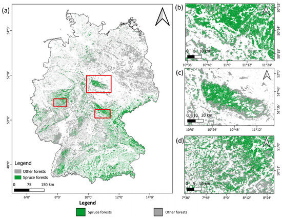
Figure 2.
(a) Forest map of Germany with study areas marked with red box. The study areas, Siegen, Harz and Frankenwald are shown in red rectangular boxes from left to right, respectively; (b) Study area Frankenwald; (c) Study area Harz; (d) Study area Siegen. The Dominant Tree Species for Germany 2018 dataset [61] was used for mapping spruce forests (green) and other forests (gray).
2.2. Data and Tools
The research utilizes the German canopy-cover-loss dataset [62] and the dominant tree species for Germany 2018 [63] as the primary data. Environmental data were used, such as temperature, elevation and spectral indices based on EO data, including Landsat 8-9 OLI/TIRS Collection 2 Level-2 [64], Surface Soil Moisture product [65] and Copernicus Digital Elevation Model GLO-30 [66]. Other environmental data were also used, such as precipitation from hydrometeorological raster datasets (HYRAS) [67] and soil texture from European Soil Data Centre (ESDAC) [68]. All data used in the study are listed in Table 1. All analysis and figures were done on Python version 3.11.9 with libraries numpy, xarray, numba, dask, tensorflow, matplotlib, gdal, scikit-learn, odc-stac, pystac-client and rioxarray. QGIS version 3.34.0 and Inkscape version 1.4 were also used for figures.

Table 1.
List of all data with source, used variable, spatial resolution, time period and reference.
2.2.1. German Canopy-Cover-Loss Dataset (2018–2024)
Thonfeld et al. [14] produced a canopy-cover-loss dataset for Germany for the time period January 2018 to April 2021 with 10 m spatial resolution and at monthly temporal resolution. The dataset uses EO time series from Landsat-8/9 and Sentinel-2A/B. The identification process involves using the disturbance index [70], which is an index calculated using tasseled cap components, brightness, greenness and wetness, calculated from the satellite data, to generate monthly composites and calculate anomalies compared to the reference period, 2017, and applying a threshold to it in order to differentiate between intact canopy and the canopy cover lost. The dataset indicates the date of the canopy cover loss. The updated version of this dataset was used in this research to obtain canopy cover loss information for a longer time period from September 2017 to September 2024 [62], which provided enough data for both training, test and validation data for our prediction model. The dataset is short in temporal interval but dense due to the monthly temporal resolution.
2.2.2. Dominant Tree Species for Germany 2018
This dataset, produced by the Thuenen institute, provides a tree species classification of all German forests. The product was created using Sentinel-1 and Sentinel-2 satellite time-series data along with environmental data [63]. The German National Forest Inventory data were used for training and validation of this dataset. Dominant species in this dataset refers to the species with the largest basal area share in the pixel area [63]. The product has an overall accuracy of 75.53%, which includes both pure-species and mixed-species stands, and 87.07% for pure-species stands only. The class-specific validation of spruce resulted in an F-score of 86.79% for all stands and 90.39% for pure stands. Using this dataset, the areas which were spruce forests prior to 2017 were identified.
2.2.3. Hydrometeorological Raster Datasets (HYRAS)
The HYRAS dataset provides data for various hydrometeorological variables for Germany. We used the raster data set “precipitation sums in mm” for Germany (HYRAS-DE-PR) [67]. This dataset is produced by the Deutscher Wetterdienst and contains daily precipitation sums in mm for Germany in a 1 × 1 km grid [67]. The dataset was generated and validated in a study by Rauthe et al. [69]. The dataset is an interpolated grid which is based on daily measured values of precipitation from weather stations using the REGNIE method. It is a robust dataset, as it undergoes quality control every month where the past month is recalculated based on quality-controlled measurements. The dataset covers the entirety of Germany for the period from 1931 to the present day. Using this dataset, a sum of precipitation for months between April and October was calculated for required years to avoid snowfall.
2.2.4. Copernicus Digital Elevation Model GLO-30
The Copernicus Digital Elevation Model GLO-30 dataset is a global digital elevation model (DEM) provided by the European Space Agency (ESA) with a spatial resolution of 30 m [66]. The DEM is based on a combination of radar and optical satellite data, including TanDEM-X. As it is the DEM with the highest spatial resolution that is openly accessible, the dataset was used to provide accurate elevation data for the relevant study areas. Other parameters extracted from the DEM, such as slope and aspect, were tested but not found to be relevant.
2.2.5. European Soil Data Centre (ESDAC)—Soil Texture
The European Soil Data Centre (ESDAC) is a database provided by the European Union (EU) for soil-related data and research [68]. From this database, a dominant surface textural class map of soil was used for our research. The map, with a 1 km spatial resolution, classifies the soil texture as coarse, medium, medium-fine, fine, very fine, no texture and no information. This dataset was used as an environmental variable to give an idea about soil properties and its ability to retain moisture.
2.2.6. Surface Soil Moisture 2014-Present (Raster 1 km), Europe, Daily
The Copernicus surface soil moisture product is based on the C-band SAR Sentinel-1 satellite data. To derive this product, Bauer-Marschallinger et al. [65] adapted a well-established change detection algorithm from TU Wien to estimate soil moisture and developed methods for spatial upscaling of SAR imagery. There is low agreement of SSM over dense vegetation, yet this dataset provides some insights on soil moisture and vegetation dynamics [65]. The spatial resolution of this product is 1 km, and the temporal resolution is daily.
2.2.7. Landsat 8-9 OLI/TIRS Collection 2 Level-2
This dataset is a collection of images from the Operational Land Imager (OLI) and Thermal Infrared Sensor (TIRS) instruments onboard the Landsat 8 (April 2013 to present) and 9 (31 January 2022 to present), satellites which have already been geometrically and radiometrically pre-processed [71]. The OLI instrument has 9 spectral bands, and the TIRS instrument has 2 thermal bands. Bands 5, 6 and 7 from the spectral bands of the OLI instrument were used to calculate spectral indices. Band 10 of the thermal infrared band from the TIRS instrument was used to measure surface temperature of the study area. The Landsat Pixel Quality Assessment was also used.
2.3. Pre-Processing and Parameterization
2.3.1. Data Initialization
The canopy-cover-loss product was first masked by the pixels of the dominant tree species dataset from Thuenen Institute, classified as spruce, to produce a spruce canopy-cover-loss raster dataset. The dominant tree species dataset was also used to create a raster dataset which only included areas with no spruce forest. This “no spruce” raster included both forested areas with other species and non-forest areas.
2.3.2. Spatio-Temporal Matrix
The Spatio-Temporal Matrix (STM) method is a pixel-based approach for data augmentation developed by Wang et al. [59] where the spatial and temporal information of neighborhood pixels is utilized. The matrix provides temporal information based on the most recent change of the pixel. It can, therefore, be an excellent tool to use with datasets that provide information on change detection or with dense time series of binary datasets. The major limitation of the STM is that it can only be used with data where the change occurs in one direction, meaning that the change from 0 to 1 is detected while the change from 1 to 0 is not. Wang et al. [59] used the STM to predict future urban/settlement growth on a yearly temporal scale. For our purposes, the method was modified to work with the spruce canopy-cover-loss dataset.
As shown in Figure 3, to develop the STM for each pixel, a continuous-period map needs to be calculated. A reference time period is set, going backwards from a reference point (denoted by ) to a temporal limit of the STM (denoted by ). A continuous-period map for the reference time period is then generated, calculating the elapsed time between an occurred change in the corresponding pixel in comparison to the reference point. Change which occurred before the reference time period is given the same values as . This map is the temporal information used in the STM.
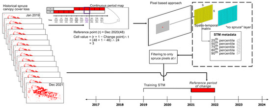
Figure 3.
Pre-processing and parameterization steps performed for calculation of STM data, “no spruce” data and reference data for each pixel used in model training.
To get the final STM for every pixel, a square window, centered on the pixel, is applied on the continuous-period map. The size of this window, denoted as , is constant and determines the extent of spatial information incorporated into the STM. By using this windowing approach, the spatial context of each pixel is captured, providing a more comprehensive understanding of the neighborhood.
The complete STM dataset has the structure , where the total number of pixels is represented by . This three-dimensional dataset contains the STM information for all pixels, with each pixel’s data organized in a matrix. This structure enables efficient storage and processing of the spatio-temporal information.
2.3.3. Adapting the STM Method to the Canopy-Cover-Loss Dataset
The STM method described above cannot immediately be applied to canopy cover loss due to the non-binary nature of the classes. The canopy-cover-loss dataset has numerical values representing dates at which canopy cover loss was recorded and zero values for intact forests and other land uses. However, the zero values represent both spruce forest area and areas without spruce forest.
To complement the STM with information about areas without spruce forest in the neighborhood, we used the “no spruce” raster. We generated spatial information for every pixel using the same windowed approach mentioned above. The window size was kept constant to allow stacking. This technique allows us to generate spatial information for every spruce pixel, characterizing the presence or absence of spruce forest in the neighborhood.
An STM window and a “no spruce” window of size can be generated for every pixel in the image. However, an additional filtering step was performed to only consider the STM and “no spruce” data of those pixels which are spruce forest at the reference time point. This step ensures that the STM and “no spruce” data are only processed for relevant pixels and not of pixels which have no spruce forests. Pixels with canopy cover loss before the reference time point are excluded, as it is unlikely that these areas have developed forests that can experience canopy cover loss again. The total number of pixels after filtering is denoted by .
While the STM provides information about importance of various locations of the neighborhood of the pixel both spatially and temporally, it does not provide information about the distribution of loss in the neighborhood. Thus, in addition to the STM, we extracted supplemental percentile information from the STM to provide background context on the neighborhood. The distribution of STM values gives us an insight into the level of canopy cover loss that was previously present in the surrounding area. Therefore, we calculated quartile values (25th, 50th and 75th percentile) of the STM. Since the STM values are more likely to be zero due to the high class imbalance caused by rarity of loss pixels, we also included the 80th and 90th percentile. They will collectively be referred to as STM metadata from here on. The STM metadata provide a concise summary of the neighborhood’s canopy-cover-loss history, allowing for a more informed prediction of future canopy cover loss in the pixel.
After testing and evaluation, we set a default window size, , of 15. This choice of window size allows us to capture the spatial context of the canopy cover loss while avoiding unnecessary computational complexity. We set the temporal limit of the STM, , to 24 months, which means that the temporal information up to 24 months before the reference point is used and any changes before that are given the maximum value of 24 months regardless of how old the loss is. The reference point is always selected in the month of December to encompass loss in two complete years.
2.3.4. Addition of Environmental Parameters from the Previous Years
In addition to the STM-augmented data, key environmental parameters are crucial for a thorough analysis and for explaining spatial heterogeneity that cannot be explained by past canopy cover loss alone [5,14,72]. However, since our aim is to predict future loss, we only look into environmental and climatic data available before the reference time point, . In this regard, we tested incorporating data that were freely available with adequate spatial resolution (<=1 km) and available for the required time period. Validation results of a model based on STM data and metadata, which will be explained later, were used to determine if the distributions of the true positives, false positives and false negatives were different for the values of the tested parameter. This would show the need or importance of integration of the features into the prediction model.
EO data, climate data and topographic data that could contribute to affect spruce vitality were tested. The exploratory analysis was conducted for topographical variables, such as elevation, slope and aspect, extracted from Copernicus DEM GLO-30, and resampled to a spatial resolution of 10 m using linear interpolation. We found that only elevation gradients were a contributing factor that exhibited a difference between the distribution of true positives, false negatives and false positives. Road accessibility was also tested, as it was assumed that for canopy cover loss caused by logging and harvesting, access to roads would be an important predictor. Open street map road layers were extracted, and pixels with road within STM boundaries were summed up to provide a layer explaining access to road for every pixel. However, we did not see a big difference between true positives, false positives and false negatives; hence, this data was excluded.
Since temperature and availability of water are the key environmental factors for tree health or forest stress, proxies to represent these variables in the past two years were also selected for exploration [5,72]. The HYRAS-DE-PR dataset was used for precipitation data to indicate availability of water, as it was the dataset with the highest spatial resolution that was accessible freely. Daily data from summer months (April to October) were summed up. The 1 km dataset was resampled to a spatial resolution of 10 m using linear interpolation. Landsat-8 data was utilized for years prior to the reference time period for summer months (April to October) after resampling to 10 m for obtaining data regarding temperature and relevant spectral indices. Poor-quality pixels were masked out using the Landsat Pixel Quality Assessment to remove erroneous pixels such as clouds, cloud shadows or snow cover. The Landsat-8 TIRS product was used to obtain surface temperature data. The Landsat-8 OLI product was used to calculate the spectral indices, Normalized Difference Moisture Index (NDMI) [73] and Normalized Multi-Band Drought Index (NMDI) [74] to represent forest health related to dryness and disturbance [75]. The dataset was filtered annually and then condensed through the calculation of percentiles, 5th, 50th, 95th. All the temperature, precipitation and spectral indices features were tested, to see if they exhibited a difference in the distribution of true positives, false negatives and false positives, and showed high feature importance. Soil properties and soil moisture were also identified as key indicators for tree health and resilience [76,77,78]. The Copernicus Surface Soil Moisture product was used after it was resampled to 10 m spatial resolution from 1 km using cubic interpolation. The soil texture data from the ESDAC was used after it was resampled to 10 m spatial resolution using nearest neighbor interpolation. In this manner, key environmental and topographic information was obtained at the highest resolution possible to give supplemental information and have a more complete and accurate prediction.
For each pixel, there are two forms of spatial input data produced, two-dimensional and one-dimensional. There are two layers with two dimensions, the STM layer and the “no spruce” layer. The one-dimensional data for each pixel includes STM metadata along with environmental and topographic information, if included. The data are used altogether as input data into the prediction model for canopy cover loss, as depicted in Figure 4. Different parameter predictor sets (Table 2) were created to test model improvement.
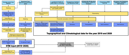
Figure 4.
Schematic diagram of preprocessing, inputs and outputs of prediction model for the period of 2021 loss. All input datasets are shown in light blue, intermediary pre-processing steps in yellow, intermediary data products in dark blue, forecasting model in dark grey and final output in light grey. Abbreviations STM: Spatio-temporal matrix; OLI: Operational Land Imager; TIRS: Thermal Infrared Sensor; HYRAS-DE-PR: Hydrometeorological raster datasets—Deutschland—precipitation sums in mm; DEM GLO-30: Global digital elevation model 30 m; RF: Random forest, MLP: Multi-layer perceptron; CNN-ANN: Convolutional Neural Network–Artificial Neural Network.
Table 2.
Different predictor sets for canopy-cover-loss prediction model and corresponding label name.
2.4. Model Training and Evaluation
2.4.1. Models Used
Most research for modeling and prediction in forests extensively uses random forest (RF) due to its ease and minimal computation requirements [79]. Simple deep neural networks such as Multi-Layer Perceptron (MLP) are also popular [59]. Now, with accelerated computing resources and speed with the use of graphical processing units (GPUs), and the formation of high-performance data analytics (HPDA) systems, there has been a resurgence of neural networks which have led to better algorithms and neural network designs [80]. The two-dimensional nature of the STM can be optimized by using a Convolution Neural Network (CNN), while the environmental parameters and the STM metadata can be put through a simple Artificial Neural Network (ANN). We tested combining the approaches to create a hybrid CNN-ANN model by concatenating the outputs of the CNN and ANN model in a combined model produced in keras library [81], as shown in Figure 5. The model architecture is explained in Table 3. The ‘relu’ activation function was used in all layers due to its compatibility with deep neural networks, except for the final layer where a ‘sigmoid’ activation function was used to give the output in the form of a probability for each class. The results of this model were compared with results of MLP and RF from the scikit-learn library [82] on the STM prediction model.
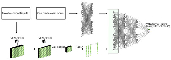
Figure 5.
Visual description of the Convolutional Neural Network–Artificial Neural Network (CNN-ANN) combined model. The model is a combined model where 2D data input and 1D data input can be provided for the same reference data. Hence, image and its metadata can be used for prediction.
Table 3.
Model architecture with size of all nodes. The model takes input parameters in two steps—the first layer of the Convolutional Neural Network (CNN) setup and the first layer of the Artificial Neural Network (ANN) setup—and gives a final output with two results, the probability of 1 (change) as a result and the probability of 0 (no change). We only use the probability of change as our final output.
The training data were generated for the years 2019 to 2020 with reference labels of spruce canopy cover loss detected in 2021. The training data were split into train and test sets where 70% of the data were used for training and 30% for test. Since the number of reference data pixels for canopy cover loss in a specific year is much lower compared to the overall spruce forests in the area, class imbalance is always going to be present. To address the class imbalance issue, class weighting was done where a weight was calculated for each class based on the reference label data. Additionally, for our CNN-ANN model, macro F1-score was used as the metric of choice, as it chooses the best model based on the precision and recall of classes rather than other metrics where the overall accuracy is more important. The model training used the Adam optimizer [83] with a learning rate of 0.001, where the learning rate dropped by a factor of 0.1 if the model plateaued in five subsequent epochs. The binary cross entropy loss function was used, as it is a commonly used loss function for binary data with probability results. The loss function quantifies the disparity between the projected probabilities and the actual labels, and adjusts the model parameters [84]. During training, the model iterated over the input dataset for 100 epochs in batches of 256 samples. However, if there is no improvement in loss of the model after 10 epochs, the training is stopped.
For different model type comparison, the input data were trained with RF and MLP and the custom CNN-ANN model without environmental parameters in the Frankenwald region. Models were trained using the CNN-ANN model in the Frankenwald region, with different predictor sets of environmental parameters as metadata, as shown in Table 2. Different time periods and different regions were tested to see if there was variation in spatial and temporal scales. Cross-validation was also conducted for models trained in different regions to test the generalization of the models.
2.4.2. Validation
The models made a prediction of canopy cover loss in 2022 based on the data generated for years 2020 and 2021 for the respective study areas. This prediction was used to test the efficiency of the model in comparison to the real canopy cover loss detected in 2022 based on the product from Thonfeld et al. [14]. The accuracy at different probability thresholds, 1% to 99%, was used to represent the effectiveness of the prediction. The prediction model was further validated using an independent dataset that was used by Reinosch et al. [85] for validating their Sentinel-2 forest disturbance maps. Validation point data showing disturbed or undisturbed forests were available for the Frankenwald forest for the year 2022.
The receiving operating characteristic (ROC) graph is a good method to compare different models and their robustness. The ROC graph plots the False Positive Rate (FPR) in the x-axis and the True Positive Rate (TPR) in the y-axis. A diagonal line where y = x represents randomness. To plot an ROC graph, binary output maps were generated for probability thresholds 1% to 99%, which were then compared to the real canopy cover loss to get a confusion matrix and subsequently calculate the TPR and FPR. A line is plotted with a point for every probability threshold. This depicts tradeoffs between true positives and false positives for any given threshold [86]. ROC space is ideal for use in imbalanced datasets, as they are not affected by class distributions. The area under the curve (AUC) of the ROC was used as the metric to compare the different models. The AUC is the portion of the area under the ROC curve.
The overall AUC of the model was calculated with TPR and FPR for all probability thresholds. Point AUC was also calculated for every probability threshold, and the best point AUC value was used as a comparison along with accuracy, precision and recall at these thresholds.
3. Results
3.1. Performance Across Different Regions in Germany
The results of models trained in different study regions (Figure 2) are shown in Figure 6, where the model output and actual canopy cover loss are compared. The model was trained on 2021 loss based on data from 2019–2020 and validated for 2020–2021 years with data of 2022 for each region separately. The model is the CNN-ANN hybrid model with STM data as predictors. The evaluation metrics are shown in Table 4 and Table 5. The results of the cross-validation of the models in different regions are shown in Table 6.
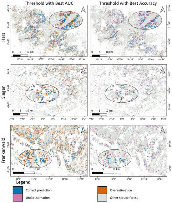
Figure 6.
Maps of predicted canopy cover loss, 2022, with different thresholds (best AUC and best Accuracy) for different regions.
Table 4.
Model evaluation results of models in different study sites with best AUC as probability threshold. Best metric is shown in bold. Each model was trained on the respective study site for loss in 2021 used the previous two years (2019–2020) and validated using loss in 2022 using the previous two years (2020–2021).
Table 5.
Model evaluation results of models in different study sites with best accuracy as probability threshold. Best metric is shown in bold. Each model was trained on the respective study site for loss in 2021 used the previous two years (2019–2020) and validated using loss in 2022 using the previous two years (2020–2021).
Table 6.
Cross-validation results of models in different study sites using Overall AUC. Best metric for region is shown in bold. The models that were trained for loss in 2021 using the previous two years (2019–2020) were cross-validated in all regions using loss in 2022 predicted using data from the previous two years (2020–2021).
3.2. Model Performance
The results of models trained in RF, MLP and a custom CNN-ANN hybrid model for the region of Frankenwald—trained on 2021 loss and validated with data of 2022, with STM data only as predictors—are shown in Table 7. The ROC curve representation along with the accuracy, precision and recall at different probability thresholds are depicted in Figure 7. The CNN-ANN model shows the best performance according to AUC metrics and has the best precision. Recall is the best in RF; however, accuracy is the worst.
Table 7.
Model evaluation across different models. Best metric is shown in bold. Each model was trained on the Frankenwald test site for loss in 2021 used the previous two years (2019–2020) and validated using loss in 2022 using the previous two years (2020–2021).
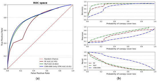
Figure 7.
(a) ROC space of different models. (b) Accuracy, precision and recall across different probability thresholds of the models. RF: Random Forest; MLP: Multi-layer perceptron; CNN-ANN: Convolutional neural network–artificial neural network; AUC: Area under curve; ROC: Receiving Operating Characteristic.
3.3. Performance Across Different Temporal Periods
The results of models evaluated in different time periods are shown in Table 8. There were two models trained, one in 2021 loss based on STM of 2019–2020 and another in 2022 loss based on STM of 2020–2021. The 2021 loss model was validated with data of 2022 and 2023, while the 2022 loss model was validated with data of 2023. The model across different temporal periods was tested for the region of Frankenwald using the CNN-ANN hybrid model with STM data as predictors.
Table 8.
Model evaluation across different years. Best metric is shown in bold. Each model was trained on the Frankenwald test site. The validation year 2022 using the previous two years (2020–2021) was trained on loss in 2021 using the previous two years (2019–2020). The validation year 2023 using the previous two years (2021–2022) had two models. One trained on loss in 2021 using the previous two years (2019–2020), another trained on loss in 2022 using the previous two years (2020–2021).
3.4. Predictor Performance
The results of model trained with different predictors sets as mentioned in Table 2 are shown in Table 9. The region of Frankenwald was used, and training was carried out on 2021 loss with STM of 2019–2020 and validated with reference data of 2022 with STM of 2020–2021 using the CNN-ANN hybrid model. The predictor set with highest AUC and recall is the M_STM_tempprecip, followed by the M_onlySTMdata. The M_STM_soilmos predictor set added to the STM parameters performs the worst. The predictor set with the best precision and accuracy at highest AUC is the M_STM_allenv. The predictors were tested for variable collinearity (Appendix A), where collinearities were only found in two expected cases, between time-lagged variables, and between indices calculated using similar bands (Table A1, Table A2 and Table A3).
Table 9.
Model evaluation results across different predictor sets. Best metric is shown in bold. Each model with different predictor set was trained on the Frankenwald test site for loss in 2021 used the previous two years (2019–2020) and validated using loss in 2022 using the previous two years (2020–2021). Best metric is shown in bold.
3.5. Independent Field Data Validation
The results of the models trained in Frankenwald region and validated using independent validation dataset from Reinosch et al. [85] are shown in Table 10. The model was trained on 2021 loss based on data from 2019–2020. We predicted for spruce canopy cover loss for 2022 using data from 2020–2021 and the CNN-ANN hybrid model with STM data as predictors. We extracted field data points from 2022 for the Frankenwald region present in the study area. The disturbed and undisturbed forest points from the field data, which in total had 688 points, were then compared to the prediction for the year 2022.
Table 10.
Model evaluation results of model in Frankenwald study site with best AUC as probability threshold. The model was trained on the respective study site for loss in 2021 used the previous two years (2019–2020) and 2022 field data points from Reinosh et al. [85] for the study site.
4. Discussion
4.1. Prediction Results
Using the STM approach, we have been able to obtain good overall AUC results compared to AUC values based on [87], on validation data (year 2022) with AUC values above 80% in all test study sites that we have (Table 4). This shows the viability of predictions using the STM approach for discrete binary datasets. To ensure that this is not an outlier year where the prediction was accurate, we also tested the model in Frankenwald region in 2023 using the same model trained on 2021 canopy cover loss as reference and a different model trained on 2022 canopy cover loss as reference. The results in different time periods showed fair model results (Table 8) with AUC values above 0.78. The reason for such prediction results, where spatio-temporal data presented by the STM for the two prior years is enough to give good forecasts of future loss, could be that the past data of the surrounding pixels explains a wide range of behaviors, such as loss of resilience in the neighborhood due to windthrow and bark beetle infestations, and the effect of forest management practices. We also found that the models can be generalized spatially (Table 6), with models trained in different regions predicting other regions fairly well.
For the purpose of using the canopy-cover-loss dataset, there is a need to use models other than the readymade models directly from scikit-learn package [82] such as RF and MLP. This is due to the fact that these models try to maximize overall accuracy. Canopy cover loss is a highly imbalanced class. While overall accuracy is important, maximizing the prediction of the canopy-cover-loss class is the priority, without overpredicting. In this regard, adjustments are made to the model architecture such as performing class weighting along with the use of macro F1-score for model selection. For the RF and MLP models, we can observe that they have their probability thresholds with best AUC at levels lower than 10% probability, even though the AUC metric looks acceptable (Table 7). Most studies use a bias correction algorithm to adjust the cumulative distribution function of the forests to observed values [53], as bias is a common feature of machine learning models; however, this is not applicable for future forecasts of variables without observed values. The MLP and RF models have faster-decreasing recall with increase in precision and probability threshold in comparison to the adjusted model, which could be attributed to the greater capacity of the CNN-ANN model to identify spatial patterns.
The external validation of the dataset achieved an overall AUC value of 0.71 (Table 10). The validation was conducted using field point data collected for the validation of Reinosch et al. [85], where disturbance maps were validated. Only a small subset of the Frankenwald region for the year 2022 (688 points) could be validated, as this was the only data available for this period of time for our study area from this dataset. We can attribute the difference in the AUC values for the validation between the canopy-cover-loss product and the disturbance validation to the different characteristics of these data and the smaller coverage of the field validation data.
4.2. Importance of Environmental Factors for the Prediction
From the literature, we know that canopy cover loss is dependent on many environmental factors, such as temperature, precipitation, soil moisture and elevation. We also know that signs for future canopy cover loss can be detected prematurely by indicators for vegetation health. However, from our tests of adding topographical and environmental variables of the two preceding years to the model in different predictor sets, we only found an improvement in AUC value in one case, when adding temperature and precipitation data (Table 9).
Temperature and availability of water in summer months of prior years are key factors that affect the disturbance regime of spruce forests [61]. The improvement to the model from these climatic variables is to be expected, as the main reason for the anomalous levels of canopy cover loss are trees weakened by drought. This makes them more susceptible to windthrow events and bark beetle outbreaks [88,89]. Therefore, the addition of these variables could potentially help the model identify such losses better.
Elevation, as the topographical variable with variation not explained by STM data, did not improve the model qualitatively. The spectral indices we used were NMDI and NDMI, which are a representation for disturbance and moisture deficiency, respectively. The model becomes more precise with this information; however, recall decreases. This may be primarily due to the canopy-cover-loss dataset already accounting for some of the variables. Canopy cover loss is based on the disturbance index, which is calculated using the tasseled cap components brightness, greenness and wetness [14]. On the other hand, the variables might confuse the model as well, by decreasing the likelihood of some correct pixels being included.
Soil moisture is broadly considered a very important factor in regards to canopy cover loss due to the fact that it is a key indicator for water deficits [76]. Yet, the historical soil moisture from two years prior to prediction worsens the model, as AUC metrics are poor (Table 9). This could possibly mean that because of the time-lag factor, historical soil moisture might not correlate as much to the soil moisture of the predicted year. Additionally, trees have deeper roots and can access water other than surface moisture. It is also well established that surface-soil-moisture products from SAR data have high estimated error in areas of forests and strong topography [65]. Soil moisture as a variable might be a predictor; however, this product does not provide improvements, due to limited spatial information and inaccuracy in dense vegetation. For more accurate results, data collected from the ground would be required, which is beyond the scope of this research.
From the results of adding different environmental and topographical variables, we see that the model based on STM only is very good, and only with some variables can it be improved. The spatio-temporal data of the canopy cover loss can therefore, be considered a sufficiently good predictor alone. In contrast to the idea that more input data equal a better model, we see that the use of more data does not improve the model significantly, which we can also see in other studies [90]. The minor increases in model performance by adding additional parameters does not justify the trade-off of the increase in computation time, which more than doubled in our approach.
4.3. Regional Spatial Heterogeneity
Forests in different regions have different characteristics. The stand density, forest management practices, forest fragmentation and species diversity in forest are all factors which can affect canopy cover loss. This explains why we find different model performance for different study sites (Table 4 and Table 5). Both Harz and Siegen perform better than Frankenwald by a wide margin. We also see this when we perform model cross-validation (Table 6), where the Harz and Siegen models can predict loss in the other region well, but not as well in Frankenwald. This might possibly be because of the spatial homogeneity in the regions. The regions in Harz and Siegen have a spatially homogenous density of canopy cover loss. Frankenwald, on the other hand, is more diverse in terms of forest structure, as stand sizes differ within the region, having both dense and sparse canopy cover, compared to the other two regions; therefore, the model has more difficulty and is prone to over- or underprediction. Another possible reason might be that there is a factor in Frankenwald that is unaccounted for in the model that is not prevalent in the other regions. These could be microclimatic differences caused by topographic complexity, differences in geology, or the change in climatic scenario in the future.
4.4. Use and Transferability
The prediction model performs an adequate task for detecting hotspots and risk areas for spruce canopy cover loss as shown in Figure 6. Based on different probability thresholds, we can make a more or less conservative prediction. In Figure 6, we see the different prediction results we get based on two different probability thresholds, best AUC and best accuracy. We observe higher overestimation in predictions with the best AUC probability threshold. This would be more useful to identify risk areas where there is a need to identify likelihood of future spruce canopy cover loss. The prediction result based on the best accuracy probability threshold had higher underestimation in all study areas. This is more important when there is a need for definitive loss prediction. The precision–recall tradeoff is highlighted in the differences that we see by taking different thresholds in Figure 7b.
Due to the use of easily available EO datasets, the implementation of forecasting of this type is only limited by computation power and not by difficulty in data collection. Other forest types, such as beech, could potentially be predicted using this method. However, it should be noted that self-learning time-series forecasting methods could be more precise for predictions where anomalous levels of canopy cover loss are not present. Fast temporal developments are predicted using this method; thus, long-term trends and cycles are not considered.
There is a possibility of use of the prediction models for forecasting of canopy cover loss in all of Germany, keeping in mind the regional differences. Other studies have modeled spruce mortality as well, with a high degree of accuracy; however, such studies utilize ground truthing data such as forest-crown-cover surveys [91] and climate data of the period they are modeling [91,92]. Forecasting of loss beyond the known time period was only possible by using modeled future climate scenarios or extrapolating the climate data to the future time series. In this regard, the approach of our research, which only uses an EO data product for canopy cover loss and past climatic data, not the climate of the year being forecasted, is significant. There is also potential to apply similar methods to other EO data products where such forecasting methods could be applicable. It is important to maximize their potential using highly scalable and efficient forecasting techniques.
4.5. Limitations
The model assumes that the development of future canopy cover loss is related to past canopy cover loss both spatially and temporally. It is assumed that the development of canopy cover loss will stay the same as the time period, , of the STM (2019–2020 for 2021 loss and 2020–2021 for 2022 loss). However, while recent historical patterns are a good predictor of canopy cover change, the model cannot account for shifts in long-term climatology and uncertainties such as anomalous weather shifts and also events such as windthrow, frost, snowbreak, fire. This model, thus, assumes that the canopy-cover-loss drivers and climate remain relatively unchanged.
Furthermore, the STM method only detects changes in one direction, from forest to forest loss. The change in forests that undergo partial or complete recovery, either naturally or via reforestation, are not captured by this method. Capturing such changes requires a more refined modelling approach along with a different canopy cover product. In addition, the recovery processes happen at a longer temporal scale than the changes associated with canopy cover loss which, in our case, are rather quick (e.g., bark beetle infestation within weeks to months vs. recovery over years to decades).
There is constant innovation happening in machine learning, so newer models might perform better, for example, Vision-Transformers [93] and Kolmogorov–Arnold Networks models [94]. Additional model adjustments can be made to address the class imbalance issue, such as utilizing under- or oversampling techniques or using different loss functions [95]. However, with this research, we break new ground by demonstrating that prediction is possible using features such as spatio-temporal matrices of discrete binary datasets.
5. Conclusions
This research demonstrates that using the spatio-temporal matrix for forecasting spruce forest canopy cover loss based on discrete data of past canopy cover loss is a viable strategy. The STM approach originally used by Wang et al. [59] for urban growth forecasting was modified and optimized to accommodate the differences in the datasets from the original application to the small but qualitative time series of canopy-cover-loss data. The method used the dense monthly canopy-cover-loss product from [62] on which training, testing and validation were conducted. Predictions were made using STM data up to two years prior to prediction for forecasting the loss of the following year. Results were obtained using evaluation metric AUC from the ROC curve where different models, predictor sets, study sites and temporal periods were tested. We found the following:
- The approach is able to generate good probability forecasts for all regions with AUC values of 81% for Frankenwald, 82% for Harz and 82.1% for Siegen. The cross-validation of the models shows how they can be generalized spatially. The lower AUC for the Frankenwald region could be attributed to external factors such as heterogenous conditions in the site, for example, geologic and topographic complexity in the site.
- The use of a combined CNN-ANN approach improved the model performance in comparison to MLP and RF. The CNN-ANN model is tailor-made for canopy-cover-loss forecasting by allowing it to extract more spatio-temporal information while dealing with class imbalance issues and removing the need for calibration.
- The model results for prediction in different temporal periods, 2022 and 2023, were good, with AUC values of 81% and 78.7%, respectively. This proves the effectiveness of the model across different years.
- Incorporating additional time-lagged environmental factors, such as temperature and availability of water, improved the model’s performance, generating the best AUC of 82.3%. However, adding more variables did not always lead to a better result, as seen when adding time-lagged soil moisture information.
- The use of different probability thresholds, such as best AUC for a bolder prediction and best accuracy for a more conservative prediction, gives us more information on spruce forest canopy-cover-loss risk.
The use and transferability of this forecasting technique is high due to its use of freely available EO data that are easily processed without requiring ground surveys that are both expensive and have spatial and temporal limitations. It can be applied straightforwardly to different regions on a regional or national scale. Improvements can be made to the approach by incorporating more information or making model adjustments. However, seeing this as a first approach in forecasting future canopy cover loss, this study has generated an effective forecasting model which has usability at different levels.
Author Contributions
Conceptualization, S.N.S. and C.K.; writing—original draft preparation, S.N.S.; writing—review and editing, S.N.S., A.D., F.T. and C.K.; visualization, S.N.S.; supervision, C.K. All authors have read and agreed to the published version of the manuscript.
Funding
This study has been supported by the German Aerospace Center (DLR) Remote Sensing Data Center (DFD) Land Surface Dynamics (LAX) department.
Data Availability Statement
The prediction maps and models are available from the corresponding author upon reasonable request.
Acknowledgments
This paper is associated with the Real-time earth Observation of fOrest dynamics and biodiversiTy (ROOT) project under the Bavarian Research Institute for Digital Transformation (bidt). We would like to express our gratitude to Jonas Koehler, Patrick Kacic, Felix Bachofer and Zhiyuan Wang, for their support throughout the research process. All model computation was done through joint high-performance data analytics (HPDA) system “terrabyte” of the German Aerospace Center (DLR) and the Leibniz Supercomputing Center (LRZ).
Conflicts of Interest
The authors declare no conflicts of interest.
Appendix A
Appendix A.1. Variable Collinearity Analysis
The prediction model used with all variables consists of data of spectral indices (NDMI, NMDI), surface temperature, precipitation, elevation, soil moisture and soil texture. We tested the variable collinearity of these variables as shown in Table A1 for Frankenwald, Table A2 for Harz and Table A3 for Siegen.
Table A1.
Correlation matrix of training data of Frankenwald trained in loss from 2021 using data from 2018–2020.
Table A1.
Correlation matrix of training data of Frankenwald trained in loss from 2021 using data from 2018–2020.
| Median Temperature 1 Year Prior | Median NDMI 1 Year Prior | Median NMDI 1 Year Prior | Median Temperature 2 Year Prior | Median NDMI 2 Year Prior | Median NMDI 2 Year Prior | Total Precipitation 1 Year Prior | Total Precipitation 2 Year Prior | Median SSM 1 Year Prior | Soil Texture | Median SSM 2 Year Prior | Elevation | |
| Median Temperature 1 year prior | 1.000 | −0.053 | −0.077 | 0.295 | −0.148 | −0.158 | 0.029 | −0.098 | −0.007 | 0.010 | −0.007 | −0.172 |
| Median NDMI 1 year prior | −0.053 | 1.000 | 0.900 | −0.154 | 0.657 | 0.618 | −0.109 | −0.055 | 0.050 | −0.104 | 0.019 | −0.046 |
| Median NMDI 1 year prior | −0.077 | 0.900 | 1.000 | −0.219 | 0.652 | 0.698 | −0.026 | 0.063 | 0.036 | −0.092 | 0.023 | 0.064 |
| Median Temperature 2 year prior | 0.295 | −0.154 | −0.219 | 1.000 | −0.219 | −0.293 | −0.337 | −0.514 | 0.035 | −0.032 | −0.086 | −0.501 |
| Median NDMI 2 year prior | −0.148 | 0.657 | 0.652 | −0.219 | 1.000 | 0.898 | −0.148 | −0.108 | 0.008 | −0.113 | −0.018 | −0.067 |
| Median NMDI 2 year prior | −0.158 | 0.618 | 0.698 | −0.293 | 0.898 | 1.000 | −0.034 | 0.048 | 0.009 | −0.089 | −0.005 | 0.048 |
| Total precipitation 1 year prior | 0.029 | −0.109 | −0.026 | −0.337 | −0.148 | −0.034 | 1.000 | 0.726 | −0.071 | 0.066 | 0.084 | 0.698 |
| Total precipitation 2 year prior | −0.098 | −0.055 | 0.063 | −0.514 | −0.108 | 0.048 | 0.726 | 1.000 | −0.052 | 0.051 | 0.095 | 0.826 |
| Median SSM 1 year prior | −0.007 | 0.050 | 0.036 | 0.035 | 0.008 | 0.009 | −0.071 | −0.052 | 1.000 | −0.100 | 0.748 | −0.115 |
| Soil texture | 0.010 | −0.104 | −0.092 | −0.032 | −0.113 | −0.089 | 0.066 | 0.051 | −0.100 | 1.000 | −0.052 | 0.055 |
| Median SSM 2 year prior | −0.007 | 0.019 | 0.023 | −0.086 | −0.018 | −0.005 | 0.084 | 0.095 | 0.748 | −0.052 | 1.000 | 0.045 |
| Elevation | −0.172 | −0.046 | 0.064 | −0.501 | −0.067 | 0.048 | 0.698 | 0.826 | −0.115 | 0.055 | 0.045 | 1.000 |
Table A2.
Correlation matrix of training data of Harz trained in loss from 2021 using data from 2018–2020.
Table A2.
Correlation matrix of training data of Harz trained in loss from 2021 using data from 2018–2020.
| Median Temperature 1 Year Prior | Median NDMI 1 Year Prior | Median NMDI 1 Year Prior | Median Temperature 2 Year Prior | Median NDMI 2 Year Prior | Median NMDI 2 Year Prior | Total Precipitation 1 Year Prior | Total Precipitation 2 Year Prior | Median SSM 1 Year Prior | Soil Texture | Median SSM 2 Year Prior | Elevation | |
| Median Temperature 1 year prior | 1.000 | 0.026 | 0.018 | 0.174 | −0.124 | −0.127 | −0.149 | −0.166 | 0.000 | −0.010 | −0.016 | −0.167 |
| Median NDMI 1 year prior | 0.026 | 1.000 | 0.954 | −0.139 | 0.535 | 0.470 | 0.000 | −0.138 | 0.131 | −0.013 | 0.079 | −0.224 |
| Median NMDI 1 year prior | 0.018 | 0.954 | 1.000 | −0.165 | 0.537 | 0.521 | 0.026 | −0.085 | 0.109 | −0.016 | 0.055 | −0.146 |
| Median Temperature 2 year prior | 0.174 | −0.139 | −0.165 | 1.000 | −0.343 | −0.364 | −0.289 | −0.265 | −0.033 | −0.043 | −0.115 | −0.222 |
| Median NDMI 2 year prior | −0.124 | 0.535 | 0.537 | −0.343 | 1.000 | 0.941 | 0.096 | −0.020 | 0.080 | 0.033 | 0.134 | −0.051 |
| Median NMDI 2 year prior | −0.127 | 0.470 | 0.521 | −0.364 | 0.941 | 1.000 | 0.146 | 0.061 | 0.061 | 0.032 | 0.115 | 0.050 |
| Total precipitation 1 year prior | −0.149 | 0.000 | 0.026 | −0.289 | 0.096 | 0.146 | 1.000 | 0.771 | 0.167 | 0.130 | 0.111 | 0.511 |
| Total precipitation 2 year prior | −0.166 | −0.138 | −0.085 | −0.265 | −0.020 | 0.061 | 0.771 | 1.000 | −0.041 | 0.134 | −0.067 | 0.769 |
| Median SSM 1 year prior | 0.000 | 0.131 | 0.109 | −0.033 | 0.080 | 0.061 | 0.167 | −0.041 | 1.000 | 0.104 | 0.844 | −0.222 |
| Soil texture | −0.010 | −0.013 | −0.016 | −0.043 | 0.033 | 0.032 | 0.130 | 0.134 | 0.104 | 1.000 | 0.079 | 0.116 |
| Median SSM 2 year prior | −0.016 | 0.079 | 0.055 | −0.115 | 0.134 | 0.115 | 0.111 | −0.067 | 0.844 | 0.079 | 1.000 | −0.162 |
| Elevation | −0.167 | −0.224 | −0.146 | −0.222 | −0.051 | 0.050 | 0.511 | 0.769 | −0.222 | 0.116 | −0.162 | 1.000 |
Table A3.
Correlation matrix of training data of Siegen trained in loss from 2021 using data from 2018–2020.
Table A3.
Correlation matrix of training data of Siegen trained in loss from 2021 using data from 2018–2020.
| Median Temperature 1 Year Prior | Median NDMI 1 Year Prior | Median NMDI 1 Year Prior | Median Temperature 2 Year Prior | Median NDMI 2 Year Prior | Median NMDI 2 Year Prior | Total Precipitation 1 Year Prior | Total Precipitation 2 Year Prior | Median SSM 1 Year Prior | Soil Texture | Median SSM 2 Year Prior | Elevation | |
| Median Temperature 1 year prior | 1.000 | −0.055 | −0.018 | 0.015 | −0.026 | 0.017 | −0.229 | −0.073 | −0.076 | −0.396 | 0.067 | 0.350 |
| Median NDMI 1 year prior | −0.055 | 1.000 | 0.953 | −0.241 | 0.541 | 0.525 | 0.075 | 0.118 | 0.060 | −0.194 | 0.130 | 0.190 |
| Median NMDI 1 year prior | −0.018 | 0.953 | 1.000 | −0.256 | 0.560 | 0.595 | 0.069 | 0.125 | 0.047 | −0.230 | 0.139 | 0.247 |
| Median Temperature 2 year prior | 0.015 | −0.241 | −0.256 | 1.000 | −0.426 | −0.423 | −0.034 | −0.077 | 0.143 | 0.260 | −0.265 | −0.478 |
| Median NDMI 2 year prior | −0.026 | 0.541 | 0.560 | −0.426 | 1.000 | 0.933 | 0.068 | 0.132 | −0.017 | −0.164 | 0.112 | 0.174 |
| Median NMDI 2 year prior | 0.017 | 0.525 | 0.595 | −0.423 | 0.933 | 1.000 | 0.077 | 0.145 | −0.020 | −0.196 | 0.123 | 0.238 |
| Total precipitation 1 year prior | −0.229 | 0.075 | 0.069 | −0.034 | 0.068 | 0.077 | 1.000 | 0.844 | 0.236 | 0.202 | 0.245 | 0.072 |
| Total precipitation 2 year prior | −0.073 | 0.118 | 0.125 | −0.077 | 0.132 | 0.145 | 0.844 | 1.000 | 0.177 | 0.043 | 0.272 | 0.211 |
| Median SSM 1 year prior | −0.076 | 0.060 | 0.047 | 0.143 | −0.017 | −0.020 | 0.236 | 0.177 | 1.000 | 0.020 | 0.372 | −0.236 |
| Soil texture | −0.396 | −0.194 | −0.230 | 0.260 | −0.164 | −0.196 | 0.202 | 0.043 | 0.020 | 1.000 | −0.191 | −0.514 |
| Median SSM 2 year prior | 0.067 | 0.130 | 0.139 | −0.265 | 0.112 | 0.123 | 0.245 | 0.272 | 0.372 | −0.191 | 1.000 | 0.280 |
| Elevation | 0.350 | 0.190 | 0.247 | −0.478 | 0.174 | 0.238 | 0.072 | 0.211 | −0.236 | −0.514 | 0.280 | 1.000 |
References
- Riedel, T. Kohlenstoffinventur 2017—Wälder in Deutschland sind eine wichtige Kohlenstoffsenke. AFZ-DerWald 2019, 14, 14–18. [Google Scholar]
- Acharya, R.P.; Maraseni, T.; Cockfield, G. Global Trend of Forest Ecosystem Services Valuation—An Analysis of Publications. Ecosyst. Serv. 2019, 39, 100979. [Google Scholar] [CrossRef]
- Chiabai, A.; Travisi, C.M.; Markandya, A.; Ding, H.; Nunes, P.A.L.D. Economic Assessment of Forest Ecosystem Services Losses: Cost of Policy Inaction. Environ. Resour. Econ. 2011, 50, 405–445. [Google Scholar] [CrossRef]
- Bundesministerium für Ernährung und Landwirtschaft (BMEL). Der Wald in Deutschland—Ausgewählte Ergebnisse der Vierten Bundeswaldinventur; Bundesministerium für Ernährung und Landwirtschaft (BMEL): Bonn, Germany, 2024. [Google Scholar]
- Holzwarth, S.; Thonfeld, F.; Kacic, P.; Abdullahi, S.; Asam, S.; Coleman, K.; Eisfelder, C.; Gessner, U.; Huth, J.; Kraus, T.; et al. Earth-Observation-Based Monitoring of Forests in Germany—Recent Progress and Research Frontiers: A Review. Remote Sens. 2023, 15, 4234. [Google Scholar] [CrossRef]
- De Brito, M.M. Compound and Cascading Drought Impacts Do Not Happen by Chance: A Proposal to Quantify Their Relationships. Sci. Total Environ. 2021, 778, 146236. [Google Scholar] [CrossRef]
- Senf, C.; Seidl, R. Persistent Impacts of the 2018 Drought on Forest Disturbance Regimes in Europe. Biogeosciences 2021, 18, 5223–5230. [Google Scholar] [CrossRef]
- Bastos, A.; Orth, R.; Reichstein, M.; Ciais, P.; Viovy, N.; Zaehle, S.; Anthoni, P.; Arneth, A.; Gentine, P.; Joetzjer, E.; et al. Vulnerability of European Ecosystems to Two Compound Dry and Hot Summers in 2018 and 2019. Earth Syst. Dyn. 2021, 12, 1015–1035. [Google Scholar] [CrossRef]
- Forzieri, G.; Girardello, M.; Ceccherini, G.; Spinoni, J.; Feyen, L.; Hartmann, H.; Beck, P.S.A.; Camps-Valls, G.; Chirici, G.; Mauri, A.; et al. Emergent Vulnerability to Climate-Driven Disturbances in European Forests. Nat. Commun. 2021, 12, 1081. [Google Scholar] [CrossRef] [PubMed]
- Forzieri, G.; Dakos, V.; McDowell, N.G.; Ramdane, A.; Cescatti, A. Emerging Signals of Declining Forest Resilience under Climate Change. Nature 2022, 608, 534–539. [Google Scholar] [CrossRef]
- Moravec, V.; Markonis, Y.; Rakovec, O.; Svoboda, M.; Trnka, M.; Kumar, R.; Hanel, M. Europe under Multi-Year Droughts: How Severe Was the 2014–2018 Drought Period? Environ. Res. Lett. 2021, 16, 034062. [Google Scholar] [CrossRef]
- Rakovec, O.; Samaniego, L.; Hari, V.; Markonis, Y.; Moravec, V.; Thober, S.; Hanel, M.; Kumar, R. The 2018–2020 Multi-Year Drought Sets a New Benchmark in Europe. Earths Future 2022, 10, e2021EF002394. [Google Scholar] [CrossRef]
- Seidl, R.; Thom, D.; Kautz, M.; Martin-Benito, D.; Peltoniemi, M.; Vacchiano, G.; Wild, J.; Ascoli, D.; Petr, M.; Honkaniemi, J.; et al. Forest Disturbances under Climate Change. Nat. Clim. Change 2017, 7, 395–402. [Google Scholar] [CrossRef] [PubMed]
- Thonfeld, F.; Gessner, U.; Holzwarth, S.; Kriese, J.; Da Ponte, E.; Huth, J.; Kuenzer, C. A First Assessment of Canopy Cover Loss in Germany’s Forests after the 2018–2020 Drought Years. Remote Sens. 2022, 14, 562. [Google Scholar] [CrossRef]
- Bundesministerium für Ernährung und Landwirtschaft (BMEL). Ergebnisse der Waldzustandserhebung 2023; Bundesministerium für Ernährung und Landwirtschaft (BMEL): Bonn, Germany, 2023. [Google Scholar]
- Thünen-Institut für Waldökosysteme Ergebnisse der Bundesweiten Waldzustandserhebung. Available online: https://wo-apps.thuenen.de/apps/wze/ (accessed on 1 February 2025).
- Bundesministerium für Ernährung und Landwirtschaft (BMEL). Ergebnisse der Bundeswaldinventur; Bundesministerium für Ernährung und Landwirtschaft (BMEL): Bonn, Germany, 2012. [Google Scholar]
- World Meteorological Organization (WMO); United Nations Environment Programme (UNEP); International Science Council (ISC); Intergovernmental Oceanographic Commission of the United Nations Educational, Scientific and Cultural Organization (IOC-UNESCO). The 2022 GCOS ECVs Requirements (GCOS 245); GCOS; World Meteorological Organization (WMO): Geneva, Switzerland, 2022; p. 244. [Google Scholar]
- U.S. Geological Survey. Landsat—Earth Observation Satellites (Ver. 1.4, August 2022); Fact Sheet; U.S. Geological Survey: Washington, DC, USA, 2015. [Google Scholar]
- Drusch, M.; Del Bello, U.; Carlier, S.; Colin, O.; Fernandez, V.; Gascon, F.; Hoersch, B.; Isola, C.; Laberinti, P.; Martimort, P.; et al. Sentinel-2: ESA’s Optical High-Resolution Mission for GMES Operational Services. Remote Sens. Environ. 2012, 120, 25–36. [Google Scholar] [CrossRef]
- National Aeronautics and Space Administration (NASA) MODIS Moderate Resolution Imaging Spectroradiometer. Available online: https://modis.gsfc.nasa.gov/about/ (accessed on 24 February 2025).
- Brooks, E.B.; Wynne, R.H.; Thomas, V.A.; Blinn, C.E.; Coulston, J.W. On-the-Fly Massively Multitemporal Change Detection Using Statistical Quality Control Charts and Landsat Data. IEEE Trans. Geosci. Remote Sens. 2014, 52, 3316–3332. [Google Scholar] [CrossRef]
- Verbesselt, J.; Zeileis, A.; Herold, M. Near Real-Time Disturbance Detection Using Satellite Image Time Series. Remote Sens. Environ. 2012, 123, 98–108. [Google Scholar] [CrossRef]
- Zhu, Z.; Woodcock, C.E.; Olofsson, P. Continuous Monitoring of Forest Disturbance Using All Available Landsat Imagery. Remote Sens. Environ. 2012, 122, 75–91. [Google Scholar] [CrossRef]
- Zhu, Z.; Woodcock, C.E. Continuous Change Detection and Classification of Land Cover Using All Available Landsat Data. Remote Sens. Environ. 2014, 144, 152–171. [Google Scholar] [CrossRef]
- Potapov, P.; Hansen, M.C.; Pickens, A.; Hernandez-Serna, A.; Tyukavina, A.; Turubanova, S.; Zalles, V.; Li, X.; Khan, A.; Stolle, F.; et al. The Global 2000-2020 Land Cover and Land Use Change Dataset Derived from the Landsat Archive: First Results. Front. Remote Sens. 2022, 3, 856903. [Google Scholar] [CrossRef]
- Hansen, M.C.; Potapov, P.V.; Moore, R.; Hancher, M.; Turubanova, S.A.; Tyukavina, A.; Thau, D.; Stehman, S.V.; Goetz, S.J.; Loveland, T.R.; et al. High-Resolution Global Maps of 21st-Century Forest Cover Change. Science 2013, 342, 850–853. [Google Scholar] [CrossRef]
- Hansen, M.C.; Krylov, A.; Tyukavina, A.; Potapov, P.V.; Turubanova, S.; Zutta, B.; Ifo, S.; Margono, B.; Stolle, F.; Moore, R. Humid Tropical Forest Disturbance Alerts Using Landsat Data. Environ. Res. Lett. 2016, 11, 034008. [Google Scholar] [CrossRef]
- Reiche, J.; Mullissa, A.; Slagter, B.; Gou, Y.; Tsendbazar, N.-E.; Odongo-Braun, C.; Vollrath, A.; Weisse, M.J.; Stolle, F.; Pickens, A.; et al. Forest Disturbance Alerts for the Congo Basin Using Sentinel-1. Environ. Res. Lett. 2021, 16, 024005. [Google Scholar] [CrossRef]
- Pickens, A.H.; Hansen, M.C.; Adusei, B.; Potapov, P.V. Sentinel-2 Forest Loss Alert (GLAD-S2) 2020. Available online: http://glad.earthengine.app/view/s2-forest-alert (accessed on 8 February 2025).
- Viana-Soto, A.; Senf, C. The European Forest Disturbance Atlas: A Forest Disturbance Monitoring System Using the Landsat Archive. Earth Syst. Sci. Data Discuss. 2024; in review. [Google Scholar] [CrossRef]
- Diniz, C.G.; Souza, A.A.D.A.; Santos, D.C.; Dias, M.C.; Luz, N.C.D.; Moraes, D.R.V.D.; Maia, J.S.A.; Gomes, A.R.; Narvaes, I.D.S.; Valeriano, D.M.; et al. DETER-B: The New Amazon Near Real-Time Deforestation Detection System. IEEE J. Sel. Top. Appl. Earth Obs. Remote Sens. 2015, 8, 3619–3628. [Google Scholar] [CrossRef]
- Radeloff, V.C.; Roy, D.P.; Wulder, M.A.; Anderson, M.; Cook, B.; Crawford, C.J.; Friedl, M.; Gao, F.; Gorelick, N.; Hansen, M.; et al. Need and Vision for Global Medium-Resolution Landsat and Sentinel-2 Data Products. Remote Sens. Environ. 2024, 300, 113918. [Google Scholar] [CrossRef]
- Durieux, A.M.; Rustowicz, R.; Sharma, N.; Schatz, J.; Calef, M.T.; Ren, C.X. Expanding SAR-Based Probabilistic Deforestation Detections Using Machine-Learning. In Proceedings of the Applications of Machine Learning 2021; Zelinski, M.E., Taha, T.M., Howe, J., Eds.; SPIE: San Diego, CA, USA, 2021; p. 6. [Google Scholar]
- Doblas, J.; Reis, M.S.; Belluzzo, A.P.; Quadros, C.B.; Moraes, D.R.V.; Almeida, C.A.; Maurano, L.E.P.; Carvalho, A.F.A.; Sant’Anna, S.J.S.; Shimabukuro, Y.E. DETER-R: An Operational Near-Real Time Tropical Forest Disturbance Warning System Based on Sentinel-1 Time Series Analysis. Remote Sens. 2022, 14, 3658. [Google Scholar] [CrossRef]
- Pišl, J.; Rußwurm, M.; Haydn Hughes, L.; Lenczner, G.; See, L.; Dirk Wegner, J.; Tuia, D. Mapping Drivers of Tropical Forest Loss with Satellite Image Time Series and Machine Learning. Environ. Res. Lett. 2024, 19, 064053. [Google Scholar] [CrossRef]
- Wu, Z.; Yan, S.; He, L.; Shan, Y. Spatiotemporal Changes in Forest Loss and Its Linkage to Burned Areas in China. J. For. Res. 2020, 31, 2525–2536. [Google Scholar] [CrossRef]
- Holzwarth, S.; Thonfeld, F.; Abdullahi, S.; Asam, S.; Da Ponte Canova, E.; Gessner, U.; Huth, J.; Kraus, T.; Leutner, B.; Kuenzer, C. Earth Observation Based Monitoring of Forests in Germany: A Review. Remote Sens. 2020, 12, 3570. [Google Scholar] [CrossRef]
- Lange, M.; Preidl, S.; Reichmuth, A.; Heurich, M.; Doktor, D. A Continuous Tree Species-Specific Reflectance Anomaly Index Reveals Declining Forest Condition between 2016 and 2022 in Germany. Remote Sens. Environ. 2024, 312, 114323. [Google Scholar] [CrossRef]
- Gnilke, A.; Sanders, T.G.M. Distinguishing Abrupt and Gradual Forest Disturbances With MODIS-Based Phenological Anomaly Series. Front. Plant Sci. 2022, 13, 863116. [Google Scholar] [CrossRef]
- Buras, A.; Rammig, A.; Zang, C.S. The European Forest Condition Monitor: Using Remotely Sensed Forest Greenness to Identify Hot Spots of Forest Decline. Front. Plant Sci. 2021, 12, 689220. [Google Scholar] [CrossRef] [PubMed]
- Koehler, J.; Kuenzer, C. Forecasting Spatio-Temporal Dynamics on the Land Surface Using Earth Observation Data—A Review. Remote Sens. 2020, 12, 3513. [Google Scholar] [CrossRef]
- Norris, J.R. Markov Chains, 1st ed.; Cambridge University Press: Cambridge, UK, 1997; ISBN 978-0-521-48181-6. [Google Scholar]
- Nay, J.; Burchfield, E.; Gilligan, J. A Machine-Learning Approach to Forecasting Remotely Sensed Vegetation Health. Int. J. Remote Sens. 2018, 39, 1800–1816. [Google Scholar] [CrossRef]
- Tadesse, T.; Wardlow, B.D.; Hayes, M.J.; Svoboda, M.D.; Brown, J.F. The Vegetation Outlook (VegOut): A New Method for Predicting Vegetation Seasonal Greenness. GIScience Remote Sens. 2010, 47, 25–52. [Google Scholar] [CrossRef]
- Wu, T.; Feng, F.; Lin, Q.; Bai, H. A Spatio-Temporal Prediction of NDVI Based on Precipitation: An Application for Grazing Management in the Arid and Semi-Arid Grasslands. Int. J. Remote Sens. 2020, 41, 2359–2373. [Google Scholar] [CrossRef]
- Marj, A.F.; Meijerink, A.M.J. Agricultural Drought Forecasting Using Satellite Images, Climate Indices and Artificial Neural Network. Int. J. Remote Sens. 2011, 32, 9707–9719. [Google Scholar] [CrossRef]
- Fernández-Manso, A.; Quintano, C.; Fernández-Manso, O. Forecast of NDVI in Coniferous Areas Using Temporal ARIMA Analysis and Climatic Data at a Regional Scale. Int. J. Remote Sens. 2011, 32, 1595–1617. [Google Scholar] [CrossRef]
- Das, M.; Ghosh, S.K. Deep-STEP: A Deep Learning Approach for Spatiotemporal Prediction of Remote Sensing Data. IEEE Geosci. Remote Sens. Lett. 2016, 13, 1984–1988. [Google Scholar] [CrossRef]
- Chen, J.; Yang, Y.; Peng, L.; Chen, L.; Ge, X. Knowledge Graph Representation Learning-Based Forest Fire Prediction. Remote Sens. 2022, 14, 4391. [Google Scholar] [CrossRef]
- Armenteras, D.; Gibbes, C.; Anaya, J.A.; Dávalos, L.M. Integrating Remotely Sensed Fires for Predicting Deforestation for REDD+. Ecol. Appl. 2017, 27, 1294–1304. [Google Scholar] [CrossRef]
- Olsson, P.-O.; Zhao, P.; Müller, M.; Mansourian, A.; Ardö, J. Combining Sentinel-2 Data and Risk Maps to Detect Trees Predisposed to and Attacked by European Spruce Bark Beetle. Remote Sens. 2024, 16, 4166. [Google Scholar] [CrossRef]
- Valle, D.; Hyde, J.; Marsik, M.; Perz, S. Improved Inference and Prediction for Imbalanced Binary Big Data Using Case-Control Sampling: A Case Study on Deforestation in the Amazon Region. Remote Sens. 2020, 12, 1268. [Google Scholar] [CrossRef]
- Kayitesi, N.M.; Guzha, A.C.; Tonini, M.; Mariethoz, G. Land Use Land Cover Change in the African Great Lakes Region: A Spatial–Temporal Analysis and Future Predictions. Environ. Monit. Assess. 2024, 196, 852. [Google Scholar] [CrossRef] [PubMed]
- Cushman, S.A.; Macdonald, E.A.; Landguth, E.L.; Malhi, Y.; Macdonald, D.W. Multiple-Scale Prediction of Forest Loss Risk across Borneo. Landsc. Ecol. 2017, 32, 1581–1598. [Google Scholar] [CrossRef]
- Poor, E.E.; Shao, Y.; Kelly, M.J. Mapping and Predicting Forest Loss in a Sumatran Tiger Landscape from 2002 to 2050. J. Environ. Manag. 2019, 231, 397–404. [Google Scholar] [CrossRef] [PubMed]
- Voight, C.; Hernandez-Aguilar, K.; Garcia, C.; Gutierrez, S. Predictive Modeling of Future Forest Cover Change Patterns in Southern Belize. Remote Sens. 2019, 11, 823. [Google Scholar] [CrossRef]
- Mauri, A.; Girardello, M.; Strona, G.; Beck, P.S.A.; Forzieri, G.; Caudullo, G.; Manca, F.; Cescatti, A. EU-Trees4F, a Dataset on the Future Distribution of European Tree Species. Sci. Data 2022, 9, 37. [Google Scholar] [CrossRef]
- Wang, Z.; Bachofer, F.; Koehler, J.; Huth, J.; Hoeser, T.; Marconcini, M.; Esch, T.; Kuenzer, C. Spatial Modelling and Prediction with the Spatio-Temporal Matrix: A Study on Predicting Future Settlement Growth. Land 2022, 11, 1174. [Google Scholar] [CrossRef]
- Marconcini, M.; Metz-Marconcini, A.; Üreyen, S.; Palacios-Lopez, D.; Hanke, W.; Bachofer, F.; Zeidler, J.; Esch, T.; Gorelick, N.; Kakarla, A.; et al. Outlining Where Humans Live, the World Settlement Footprint 2015. Sci. Data 2020, 7, 242. [Google Scholar] [CrossRef]
- Senf, C.; Buras, A.; Zang, C.S.; Rammig, A.; Seidl, R. Excess Forest Mortality Is Consistently Linked to Drought across Europe. Nat. Commun. 2020, 11, 6200. [Google Scholar] [CrossRef] [PubMed]
- German Aerospace Center (DLR) Forest Canopy Cover Loss (FCCL)—Germany—Monthly, 10m. 2025. Available online: https://geoservice.dlr.de/data-assets/ef9wwc5sff75.html (accessed on 10 January 2025).
- Blickensdörfer, L.; Oehmichen, K.; Pflugmacher, D.; Kleinschmit, B.; Hostert, P. National Tree Species Mapping Using Sentinel-1/2 Time Series and German National Forest Inventory Data. Remote Sens. Environ. 2024, 304, 114069. [Google Scholar] [CrossRef]
- Earth Resources Observation and Science (EROS) Center Landsat 8-9 Operational Land Imager/Thermal Infrared Sensor Level-2, Collection 2 2013. Available online: https://www.usgs.gov/centers/eros/science/usgs-eros-archive-landsat-archives-landsat-8-9-olitirs-collection-2-level-2 (accessed on 24 February 2025).
- Bauer-Marschallinger, B.; Freeman, V.; Cao, S.; Paulik, C.; Schaufler, S.; Stachl, T.; Modanesi, S.; Massari, C.; Ciabatta, L.; Brocca, L.; et al. Toward Global Soil Moisture Monitoring with Sentinel-1: Harnessing Assets and Overcoming Obstacles. IEEE Trans. Geosci. Remote Sens. 2019, 57, 520–539. [Google Scholar] [CrossRef]
- European Space Agency; Airbus Copernicus DEM 2022. Available online: https://dataspace.copernicus.eu/explore-data/data-collections/copernicus-contributing-missions/collections-description/COP-DEM (accessed on 8 January 2025).
- Deutscher Wetterdienst Raster Data Set Precipitation Sums in Mm for Germany—HYRAS-DE-PR, Version v6.0 2024. Available online: https://opendata.dwd.de/climate_environment/CDC/grids_germany/daily/hyras_de/precipitation (accessed on 8 January 2025).
- Panagos, P.; Van Liedekerke, M.; Borrelli, P.; Köninger, J.; Ballabio, C.; Orgiazzi, A.; Lugato, E.; Liakos, L.; Hervas, J.; Jones, A.; et al. European Soil Data Centre 2.0: Soil Data and Knowledge in Support of the EU Policies. Eur. J. Soil Sci. 2022, 73, e13315. [Google Scholar] [CrossRef]
- Rauthe, M.; Steiner, H.; Riediger, U.; Mazurkiewicz, A.; Gratzki, A. A Central European Precipitation Climatology Part I: Generation and Validation of a High-Resolution Gridded Daily Data Set (HYRAS). Meteorol. Z. 2013, 22, 235–256. [Google Scholar] [CrossRef]
- Healey, S.; Cohen, W.; Zhiqiang, Y.; Krankina, O. Comparison of Tasseled Cap-Based Landsat Data Structures for Use in Forest Disturbance Detection. Remote Sens. Environ. 2005, 97, 301–310. [Google Scholar] [CrossRef]
- Crawford, C.J.; Roy, D.P.; Arab, S.; Barnes, C.; Vermote, E.; Hulley, G.; Gerace, A.; Choate, M.; Engebretson, C.; Micijevic, E.; et al. The 50-Year Landsat Collection 2 Archive. Sci. Remote Sens. 2023, 8, 100103. [Google Scholar] [CrossRef]
- Nordkvist, M.; Eggers, J.; Fustel, T.L.-A.; Klapwijk, M.J. Development and Implementation of a Spruce Bark Beetle Susceptibility Index: A Framework to Compare Bark Beetle Susceptibility on Stand Level. Trees For. People 2023, 11, 100364. [Google Scholar] [CrossRef]
- Hislop, S.; Jones, S.; Soto-Berelov, M.; Skidmore, A.; Haywood, A.; Nguyen, T. Using Landsat Spectral Indices in Time-Series to Assess Wildfire Disturbance and Recovery. Remote Sens. 2018, 10, 460. [Google Scholar] [CrossRef]
- Wang, L.; Qu, J.J. NMDI: A Normalized Multi-band Drought Index for Monitoring Soil and Vegetation Moisture with Satellite Remote Sensing. Geophys. Res. Lett. 2007, 34, 2007GL031021. [Google Scholar] [CrossRef]
- Jin, S.; Sader, S.A. Comparison of Time Series Tasseled Cap Wetness and the Normalized Difference Moisture Index in Detecting Forest Disturbances. Remote Sens. Environ. 2005, 94, 364–372. [Google Scholar] [CrossRef]
- Xu, C.; Förster, M.; Beckschäfer, P.; Talkner, U.; Klinck, C.; Kleinschmit, B. Modeling European Beech Defoliation at a Regional Scale Gradient in Germany from Northern Lowlands to Central Uplands Using Geo-Ecological Parameters, Sentinel-2 and National Forest Condition Survey Data. For. Ecol. Manag. 2025, 576, 122383. [Google Scholar] [CrossRef]
- Marini, L.; Ayres, M.P.; Battisti, A.; Faccoli, M. Climate Affects Severity and Altitudinal Distribution of Outbreaks in an Eruptive Bark Beetle. Clim. Change 2012, 115, 327–341. [Google Scholar] [CrossRef]
- Netherer, S.; Matthews, B.; Katzensteiner, K.; Blackwell, E.; Henschke, P.; Hietz, P.; Pennerstorfer, J.; Rosner, S.; Kikuta, S.; Schume, H.; et al. Do Water-limiting Conditions Predispose Norway Spruce to Bark Beetle Attack? New Phytol. 2015, 205, 1128–1141. [Google Scholar] [CrossRef]
- Wittich, D.; Rottensteiner, F.; Voelsen, M.; Heipke, C.; Müller, S. Deep Learning for the Detection of Early Signs for Forest Damage Based on Satellite Imagery. ISPRS Ann. Photogramm. Remote Sens. Spat. Inf. Sci. 2022, V-2-2022, 307–315. [Google Scholar] [CrossRef]
- Vasilev, I. Python Deep Learning—Understand How Deep Neural Networks Work and Apply Them to Real-World Tasks, 3rd ed.; Packt Publishing Limited: Birmingham, UK, 2023; ISBN 978-1-83763-345-6. [Google Scholar]
- Chollet, F. Keras 2015. Available online: http://keras.io (accessed on 3 January 2025).
- Pedregosa, F.; Varoquaux, G.; Gramfort, A.; Michel, V.; Thirion, B.; Grisel, O.; Blondel, M.; Prettenhofer, P.; Weiss, R.; Dubourg, V.; et al. Scikit-Learn: Machine Learning in Python. J. Mach. Learn. Res. 2011, 12, 2825–2830. [Google Scholar]
- Kingma, D.P.; Ba, J. Adam: A Method for Stochastic Optimization. arXiv 2014. [Google Scholar] [CrossRef]
- Ndama, O.; Bensassi, I.; En-Naimi, E.M. Optimizing Credit Card Fraud Detection: A Deep Learning Approach to Imbalanced Datasets. Int. J. Electr. Comput. Eng. IJECE 2024, 14, 4802–4814. [Google Scholar] [CrossRef]
- Reinosch, E.; Backa, J.; Adler, P.; Deutscher, J.; Eisnecker, P.; Hoffmann, K.; Langner, N.; Puhm, M.; Rüetschi, M.; Straub, C.; et al. Detailed Validation of Large-Scale Sentinel-2-Based Forest Disturbance Maps across Germany. For. Int. J. For. Res. 2025, 98, 437–453. [Google Scholar] [CrossRef]
- Fawcett, T. An Introduction to ROC Analysis. Pattern Recognit. Lett. 2006, 27, 861–874. [Google Scholar] [CrossRef]
- Swets, J.A. Measuring the Accuracy of Diagnostic Systems. Science 1988, 240, 1285–1293. [Google Scholar] [CrossRef] [PubMed]
- Hlásny, T.; Zimová, S.; Merganičová, K.; Štěpánek, P.; Modlinger, R.; Turčáni, M. Devastating Outbreak of Bark Beetles in the Czech Republic: Drivers, Impacts, and Management Implications. For. Ecol. Manag. 2021, 490, 119075. [Google Scholar] [CrossRef]
- Hlásny, T.; Krokene, P.; Liebhold, A.; Montagné-Huck, C.; Müller, J.; Qin, H.; Raffa, K.; Schelhaas, M.-J.; Seidl, R.; Svoboda, M.; et al. Living with Bark Beetles: Impacts, Outlook and Management Options; From Science to Policy; European Forest Institute: Joensuu, Finland, 2019. [Google Scholar]
- Zambrano, F.; Vrieling, A.; Nelson, A.; Meroni, M.; Tadesse, T. Prediction of Drought-Induced Reduction of Agricultural Productivity in Chile from MODIS, Rainfall Estimates, and Climate Oscillation Indices. Remote Sens. Environ. 2018, 219, 15–30. [Google Scholar] [CrossRef]
- Knapp, N.; Wellbrock, N.; Bielefeldt, J.; Dühnelt, P.; Hentschel, R.; Bolte, A. From Single Trees to Country-Wide Maps: Modeling Mortality Rates in Germany Based on the Crown Condition Survey. For. Ecol. Manag. 2024, 568, 122081. [Google Scholar] [CrossRef]
- Anders, T.; Hetzer, J.; Knapp, N.; Forrest, M.; Langan, L.; Tölle, M.H.; Wellbrock, N.; Hickler, T. Modelling Past and Future Impacts of Droughts on Tree Mortality and Carbon Storage in Norway Spruce Stands in Germany. Ecol. Model. 2025, 501, 110987. [Google Scholar] [CrossRef]
- Han, K.; Wang, Y.; Chen, H.; Chen, X.; Guo, J.; Liu, Z.; Tang, Y.; Xiao, A.; Xu, C.; Xu, Y.; et al. A Survey on Vision Transformer. IEEE Trans. Pattern Anal. Mach. Intell. 2023, 45, 87–110. [Google Scholar] [CrossRef] [PubMed]
- Liu, Z.; Wang, Y.; Vaidya, S.; Ruehle, F.; Halverson, J.; Soljačić, M.; Hou, T.Y.; Tegmark, M. KAN: Kolmogorov-Arnold Networks. arXiv 2025. [Google Scholar] [CrossRef]
- Terven, J.; Cordova-Esparza, D.M.; Ramirez-Pedraza, A.; Chavez-Urbiola, E.A.; Romero-Gonzalez, J.A. Loss Functions and Metrics in Deep Learning. arXiv 2024. [Google Scholar] [CrossRef]
Disclaimer/Publisher’s Note: The statements, opinions and data contained in all publications are solely those of the individual author(s) and contributor(s) and not of MDPI and/or the editor(s). MDPI and/or the editor(s) disclaim responsibility for any injury to people or property resulting from any ideas, methods, instructions or products referred to in the content. |
© 2025 by the authors. Licensee MDPI, Basel, Switzerland. This article is an open access article distributed under the terms and conditions of the Creative Commons Attribution (CC BY) license (https://creativecommons.org/licenses/by/4.0/).