Online Sparse Reconstruction for Real Aperture Radar by Beam Recursive-Sliding Updating Framework

Abstract

Real aperture radar (RAR) can acquire the forward-looking target scene of interest continuously in scanning mode by arbitrary imaging geometry; however, the achievable angular resolution is predominantly governed by the physical dimensions of the antenna’s aperture. In contemporary radar imaging methodologies, the reconstruction of sparsely distributed targets can be effectively formulated as an $L_1$-regularized optimization framework through the exploitation of a priori sparsity constraints, thereby enabling the generation of enhanced-resolution forward-looking radar imagery. Nevertheless, traditional target reconstruction methods based on the sparse regularization framework are implemented after batch data collection, which comes at the cost of significant operational complexity and storage space. To address this challenge, an online sparse reconstruction method based on a beam recursive-sliding (BRS) updating framework is proposed to achieve fast target reconstruction. First, the antenna measurement matrix is repaired to reduce the imaging edge information error. Then, due to the independence of the echo data within two beamwidths, a beam recursive updating method is proposed for each two beamwidths echo data by the structural properties of the repaired antenna measurement matrix. Finally, based on the proposed beam recursive updating method, a sliding updating approach is proposed for the whole imaging region to reduce the computational redundancy and storage requirement. Simulation and experimental data demonstrate the effectiveness of the proposed BRS updating framework.

1. Introduction

In the forward-looking region, high-resolution radar imaging serves as a vital component in both defense and civil application, such as autonomous landing, aerial supply drops, ground mapping, and regional navigation [1,2,3,4]. However, traditional Doppler beam sharpening (DBS) and Synthetic Aperture Radar (SAR) techniques are unable to achieve high-resolution radar imaging results in the forward-looking region due to Doppler ambiguity [5,6]. Real aperture radar (RAR) typically benefits from its scanning mode to achieve imaging by arbitrary observation geometry, which enables high-range resolution through the transmission of chirp signals with a wide bandwidth. However, its azimuth resolution is typically limited by the size of its antenna aperture, resulting in comparatively coarse resolution [7,8,9]. Consequently, enhancing the angular resolution capability emerges as a critical technical requirement.

In RAR scanning mode, the azimuthal echo can be mathematically modeled as the convolution between the target scattering coefficients and the antenna pattern [10,11,12]. However, caused by the underdetermined antenna measurement matrix, target reconstruction is equivalent to a pathological inverse problem.

To reconstruct target scenes, a substantial number of super-resolution methods have been proposed. In [13,14,15,16], a sparse Bayesian framework-based target reconstruction method is developed. The method enhances angular resolution by assuming statistical prior distributions for both the target and noise. Unfortunately, it is sensitive to noise and may struggle to reconstruct target scenes in the low-SNR environments. To reduce noise influence, a truncated singular value decomposition (TSVD)-based approach is introduced in [17,18,19], and the authors obtain an approximate solution by truncating the singular value components most affected by noise. Nevertheless, the enhancement in angular resolution is inherently constrained. In [20], a Tikhonov-regularized solution framework is developed through systematic modification of the steering matrix’s singular value spectrum, where the regularization parameter is chosen manually. However, the angular resolution enhancement is functionally equivalent to that of the TSVD method.

Due to the mathematical similarities, many scholars introduce array signal processing methods into RAR imaging to obtain robust target scene reconstruction results [9,21]. Wiener filtering is a classic signal processing method for enhancing resolution [22,23]. But this method has poor performance in low-SNR environments. To address the limitations of Wiener filtering, a Spectral Iterative Adaptive Approach (IAA) method is introduced [24]. The method has demonstrated good robustness and effective noise suppression capabilities in various environments, but it requires multiple inversion of high-dimensional matrices, resulting in significant time costs. To address this problem, a Fast IAA method by exploiting the block-triangular structure of the echo autocorrelation matrix is further proposed in [25]. While retaining good super-resolution performance, this method has lower computational complexity. However, its fixed number of iterations per range bin undoubtedly leads to computational redundancy. To address the drawback of slow convergence in the IAA algorithm, a range recursive IAA algorithm is proposed in [26], based on the correlation of adjacent echoes. This algorithm effectively addresses the issue of iterative redundancy, but its computational complexity increases as the number of azimuthal sampling points increases.

When sparse targets in the forward-looking region are typically the object of interest, RAR super-resolution reconstruction can be equivalently considered as sparse reconstruction problem [27,28,29,30,31]. The enhancement of angular resolution can be modeled by introducing target prior information under a regularization framework [32,33]. The core of sparse regularization methods lies in selecting appropriate target prior information. To emphasize the sparsity of targets in the scene, most studies choose the $L_1$ norm as the constraint term within the regularization framework [34,35]. To solve the non-differentiable $L_1$ regularization problem, iterative reweighted algorithm [36], split Bregman algorithm [37,38], iterative shrinkage threshold algorithm [39], augmented Lagrange algorithm [40], and majorization–minimization (MM) algorithm [41,42] are usually used. However, the above-mentioned methods focus on batch data processing, requiring a large amount of storage space, and may introduce delays due to data collection. As the radar beam systematically scans the imaging region, the increase in data dimensions significantly raises storage requirements and acquisition time. To reduce storage requirements, decrease latency, and achieve real-time imaging, an online reconstruction method based on sparse $L_1$ regularization is proposed [43,44]. However, this method fails to account for the physical correspondence between echo pulses and target grids inherent in the beam-scanning process. The iteration relationship remains fixed, resulting in a significant amount of computational redundancy.

In this paper, an online sparse reconstruction method based on a beam recursive-sliding (BRS) updating framework is proposed to achieve low storage requirements and low latency. First, the antenna measurement matrix is repaired to reduce imaging edge information errors. Then, since the echo signals return from adjacent beamwidths intervals are statistically uncorrelated, the structural properties of the repaired antenna measurement matrix can be utlized to achieve local beam recursive updates. Finally, global beam recursive updating can be achieved through overlap shifting processing to effectively recover the target. Building upon the proposed method, the effective utilization of the correspondence between echo samples and target grid is achieved. While preserving the inherent advantages of the online framework, this algorithm effectively reduces the significant computational redundancy present in traditional online sparse reconstruction methods.

The organizational framework of this paper is presented as follows. Section 2 formulates the RAR signal model and related works are introduced. In Section 3, the proposed method is analyzed in detail. In Section 4 and Section 5, to verify the advantage of the proposed method, the simulated and experimental results are presented, respectively. Finally, Section 6 summarizes this paper and presents the conclusions.

2. Azimuth Echo Model and Related Work

The top and side views of the airbone RAR forward-looking imaging geometry model are presented in Figure 1a,b. And as illustrated in Figure 1b, the airborne flies along the y-axis direction, and the z-axis is altitude direction. $\omega$ is antenna scanning speed, v is carrier platform speed, $\beta$ is pitch angle, and H is vertical height of the carrier. In addition, ${\theta }_0$ and $R_0$ are the azimuthal angle and range history at the starting moment, respectively. At time t, $\theta \left(t\right)={\theta }_0+\omega t$ and $R\left(t\right)$ denote the azimuthal angle and range history, respectively.

In Figure 1b, target P has a range history that is indicated as

$$\begin{array}{c}R\left(t\right)=\sqrt{R_0^2+v^2{t}^2-2R_{0}vtcos{\theta }_{0}cos\beta }\end{array}$$

(1)

By applying Taylor series approximation to the above equation, we obtain

$$\begin{array}{c}R\left(t\right)\approx R_0-vtcos{\theta }_{0}cos\beta \end{array}$$

(2)

Meanwhile, RAR, while operating, transmits a chirp signal. Upon completing the scanning process, received echo is represented as

$$\begin{array}{c}\begin{array}{c}y\left(\tau ,t\right)={\displaystyle {\displaystyle \sum _{j=1}^M}}{\displaystyle {\displaystyle \sum _{i=1}^N}}{x}_{ij}\mathrm{rect}\left({\displaystyle \frac{\tau -{\tau }_d}{T}}\right)w\left(t\right)\\ exp\left[j\pi K_p{\left(\tau -{\tau }_d\right)}^2\right]exp\left(-j\pi {\displaystyle \frac{4R\left(t\right)}{\lambda }}\right)\end{array}\end{array}$$

(3)

where $y\left(·\right)$ signifies the received echo signal whereas t corresponds to the time in the azimuthal dimension. The time in the range dimension, denoted as $\tau$, is related to the speed of light. Meanwhile, M and N represent the number of sampling points in the range and azimuth directions, respectively. 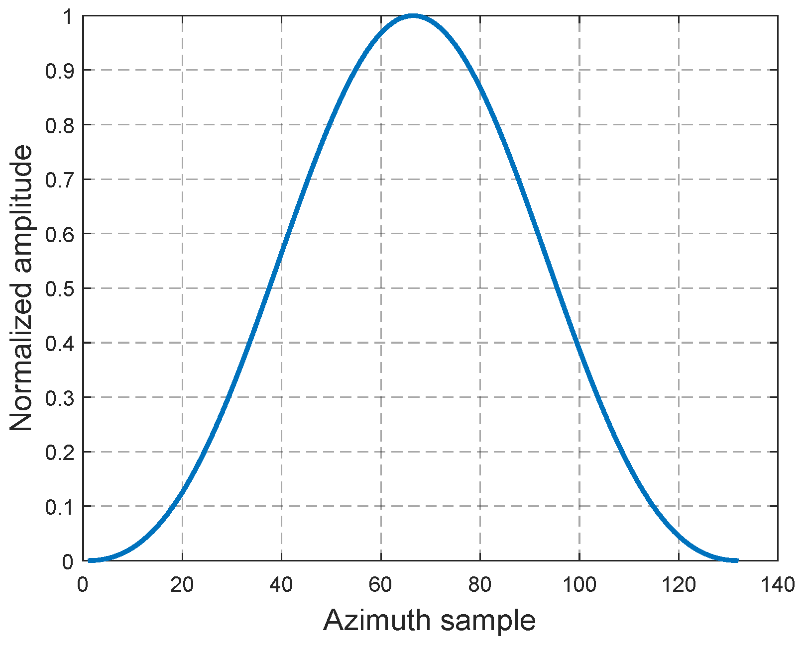And $x_{ji}$ corresponds to amplitude of the $\left(j,i\right)$th target, $\lambda$ is wavelength, $w\left(t\right)$ is antenna pattern function, which can be expressed in terms of spatial variables as $w\left(t\right)=a\left(\theta -{\theta }_0\right)$, $f_0$ is carrier frequency, $rect\left(·\right)$ refers to rectangular window function, T denotes the pulse width, $K_p$ is the linear tuning frequency, and ${\tau }_d=2R\left(t\right)/c$ denotes the time delay.

After applying pulse compression and range walk correction to echo signal in model (3) and utilizing $w\left(t\right)=a\left(\theta -{\theta }_0\right)$ and $\tau =2R/c$, it can be further represented as

$$\begin{array}{c}\begin{array}{c}y\left(R,\theta \right)={\displaystyle \sum _{j=1}^M}{\displaystyle \sum _{i=1}^N}{x}_{ji}a\left({\theta }_i-{\theta }_0\right)\mathrm{sinc}\left[{\displaystyle \frac{2B}{c}}\left(R-R_0\right)\right]\hfill \\ exp\left[-j2\pi f_0{\tau }_d\right]\hfill \end{array}\end{array}$$

(4)

The range walk correction enables the decoupling of the range and azimuth directions, and the range and azimuth echoes can be processed separately. According to Model (4), the Doppler shift $exp\left[-j2\pi f_0{\tau }_d\right]$ can be further written as $exp\left[-j{\displaystyle \frac{4\pi }{\lambda }}\left(R_0-vtcos{\theta }_{0}cos\beta \right)\right]$. As a result, the Doppler shift in any direction in the forward looking region $\left[-10°,10°\right]$ is almost the same when the platform is low-speed, which can be neglected in practical applications. Meanwhile, to clearly reveal the convolutional characteristics of the azimuth echo signal, the azimuth signal of an arbitrary range bin, when observed along the azimuth direction, can be expressed as

$$\begin{array}{c}y\left(\theta \right)={\displaystyle \sum _{i=1}^N}{x}_{i}a\left({\theta }_i-{\theta }_0\right)\end{array}$$

(5)

where $a\left({\theta }_i\right)$ denotes the sampling intensity of the $i$th sampling point of the antenna pattern function. The above expression can be further rewritten in a convolutional form, and by considering additive white noise, it becomes

$$\begin{array}{c}y\left(\theta \right)=x\left(\theta \right)\ast a\left(\theta \right)+n\left(\theta \right)\end{array}$$

(6)

where ∗ denotes convolution operation.

Therefore, in practical applications, for computational convenience, the signal is discretized, and the mth range bin’s echo can then be written in a convoluted form as follows:

$$\begin{array}{c}\mathbf{y}=\mathbf{Ax}+\mathbf{n}\end{array}$$

(7)

where $\mathbf{y}={\left[\begin{array}{cccc}{y}_1\hfill & y_2& \dots & y_N\end{array}\right]}^T\in {\mathbb{C}}^{N\times 1}$ denotes the echo dates, $\mathbf{x}={\left[\begin{array}{cccc}{x}_1\hfill & x_2& \dots & x_N\end{array}\right]}^T\in {\mathbb{C}}^{N\times 1}$ denotes the target scatterings, and $\mathbf{n}\in {\mathbb{C}}^{N\times 1}$ denotes zero-mean Gaussian white noise. The antenna measurement matrix, denoted as $\mathbf{A}$, can be expressed as follows:

$$\mathbf{A}={\left[\begin{array}{c}{a}_{\left({\theta }_{L/2}\right)}\dots a_{\left({\theta }_L\right)}\hfill \\ ⋮\ddots \ddots \hfill \\ a_{\left({\theta }_1\right)}\ddots a_{\left({\theta }_L\right)}\hfill \\ \ddots \ddots \ddots \hfill \\ a_{\left({\theta }_1\right)}\ddots a_{\left({\theta }_L\right)}\hfill \\ \ddots \ddots ⋮\hfill \\ a_{\left({\theta }_1\right)}\dots a_{\left({\theta }_{L/2}\right)}\hfill \end{array}\right]}_{N\times N}$$

(8)

where the samples of the mainlobe antenna pattern are represented by $\left[a_{\left({\theta }_1\right)}\dots a_{\left({\theta }_{L/2}\right)}\dots a_{\left({\theta }_L\right)}\right]$, the sampling index L is fundamentally governed by three key system parameters: Pulse Repetition Frequency (PRF), angular beamwidth (${\theta }_{\beta }$), and antenna’s angular scanning rate $\omega$, as expressed by relationship, i.e., $L={\theta }_{\beta }\ast PRF/\omega$.

To address the aforementioned challenges, prior research has explored various approaches. In this paper, we first introduce the traditional batch processing sparse $L_1$ regularization method; then, we further deduced its online structure.

2.1. Batch Processing Sparse $L_1$ Regularization Method

Since the relationship between echoes and targets is shown in (7), the target reconstruction problem is framed as an optimal estimation problem

$$\begin{array}{c}\underset{\mathbf{x}}{argmin}{∥\mathbf{y}-\mathbf{Ax}∥}_2^2\end{array}$$

(9)

where (9) corresponds to the least-square solution [45] which implements the $L_2$ norm to regularization to constrain the noise variance. Nevertheless, this is an underdetermined problem, which cannot be directly solved.

To enhance angular resolution, in recent years, based on the sparse characteristics of targets, the Lasso model [46], by introducing the $L_1$ norm as a constraint term within the regularization framework, can be represented as

$$\begin{array}{c}\widehat{\mathbf{x}}=\underset{\mathbf{x}}{argmin}{∥\mathbf{y}-\mathbf{Ax}∥}_2^2+\lambda {∥\mathbf{x}∥}_1\end{array}$$

(10)

where regularization parameter $\lambda$ governs the weight added to the constraint term. The MM principle, which converts the non-differentiable issue into a smooth one, can be applied to solve the Lasso model in (10).

Due to the MM principle [47], the second term in (10) can be equivalently represented as

$$\begin{array}{c}\lambda {∥\mathbf{x}∥}_1=\lambda {\mathbf{x}}^T{\mathbf{W}}_k\mathbf{x}\end{array}$$

(11)

where ${\mathbf{W}}_k=\mathrm{diag}\left(1/\left|{\mathbf{x}}_k\right|\right)$ denotes diagonal loading matrix, ${\mathbf{x}}_k$ is the result of the kth iteration for the target.

Thus, Model (10) is further expressed as

$$\begin{array}{c}{\widehat{\mathbf{x}}}^{k+1}=\underset{\mathbf{x}}{argmin}{∥\mathbf{y}-\mathbf{Ax}∥}_2^2+\lambda {\mathbf{x}}^T{\mathbf{W}}_k\mathbf{x}\end{array}$$

(12)

And it can be obtained by calculating the iterative formula as follows:

$$\begin{array}{c}{\widehat{\mathbf{x}}}^{k+1}={\left({\mathbf{A}}^T\mathbf{A}+{\mathbf{W}}_k\right)}^{-1}{\mathbf{A}}^T\mathbf{y}\end{array}$$

(13)

The batch processing sparse $L_1$ regularization method requires multiple iterations to achieve convergence. And each iteration involves matrix inversion, leading to increased storage requirements and lag in imaging for the RAR system.

2.2. Online Reconstruction Method Based on Sparse $L_1$ Regularization

To reduce storage requirements, decrease latency, and achieve real-time imaging, an online structure for the batch processing sparse $L_1$ regularization approach is further proposed in [43,44].

First, the antenna measurement matrix $\mathbf{A}$ is divided into rows. Then, it follows that $\mathbf{A}={\left[\begin{array}{cccc}{\mathbf{a}}_{\mathbf{1}};\hfill & {\mathbf{a}}_{\mathbf{2}};& \dots & {\mathbf{a}}_{\mathbf{N}}\end{array}\right]}^T$, where $a_{\mathbf{n}}{\in }^{1\times N}$ denotes the nth row vector of $\mathbf{A}$. Based on (10), to perform online sparse estimation, it would be natural to solve

$$\begin{array}{c}{\widehat{\mathbf{x}}}_{n+1}=\underset{\mathbf{x}}{argmin}{\displaystyle \sum _{j=1}^n}{\left(y_j-{\mathbf{a}}_j\mathbf{x}\right)}^2+\lambda {∥\mathbf{x}∥}_1\end{array}$$

(14)

where $y_j$ denotes the jth element of the echo $\mathbf{y}$, corresponding to the echo value at the jth azimuth sampling instant.

From the above analysis, (14) can be reformulated in an equivalent form as

$$\begin{array}{c}{\widehat{\mathbf{x}}}_{n+1}=\underset{\mathbf{x}}{argmin}{\displaystyle \sum _{j=1}^n}{\left(y_j-{\mathbf{a}}_j\mathbf{x}\right)}^2+\lambda {\mathbf{x}}^T{\mathbf{W}}_n\mathbf{x}\end{array}$$

(15)

Here, ${\mathbf{W}}_{\mathrm{n}}=\mathrm{diag}\left(1/\left|{\mathbf{x}}_n\right|\right)$, and ${\widehat{\mathbf{x}}}_{n+1}$ represents estimated real-time target scattering coefficients when the $n+1$th echo arrives. And the following equation provides the closed-form solution to (15).

$$\begin{array}{c}{\widehat{\mathbf{x}}}_{n+1}={\left(\lambda {\mathbf{W}}_n+{\displaystyle \sum _{j=1}^n}{\mathbf{a}}_j^T{\mathbf{a}}_j\right)}^{-1}\left({\displaystyle \sum _{j=1}^n}{\mathbf{a}}_j^T{y}_j\right)\end{array}$$

(16)

For the solution in (16), we let ${\mathbf{b}}_n={\displaystyle \sum _{j=1}^n}{\mathbf{a}}_j^T{y}_j$, ${\mathbf{Q}}_n={\displaystyle \sum _{j=1}^n}{\mathbf{a}}_j^T{\mathbf{a}}_j$, then ${\mathbf{A}}_n=\lambda {\mathbf{W}}_n+{\mathbf{Q}}_n$. Thus, (16) can be written as

$$\begin{array}{c}\mathbf{x}={\mathbf{A}}_n^{-1}{\mathbf{b}}_n\end{array}$$

(17)

For the recursion initialization at $n=1$, the initialization vector takes the form

$$\begin{array}{c}\begin{array}{c}{\mathbf{Q}}_1={\mathbf{a}}_1^T{\mathbf{a}}_1\hfill \\ {\mathbf{b}}_1={\mathbf{a}}_1^T{y}_1\hfill \\ {\mathbf{W}}_1=\mathbf{I}\hfill \end{array}\end{array}$$

(18)

The terminal recursion step at $n\ge 2$ is calculated by the following formula:

$$\begin{array}{c}\begin{array}{c}{\mathbf{Q}}_n={\mathbf{Q}}_{n-1}+{\mathbf{a}}_n^T{\mathbf{a}}_n\hfill \\ {\mathbf{b}}_n={\mathbf{b}}_{n-1}+{\mathbf{a}}_n^T{y}_n\hfill \\ {\mathbf{W}}_n=\mathrm{diag}\left(1/\left|{\mathbf{x}}_n\right|\right)\hfill \end{array}\end{array}$$

(19)

Through the above derivation, we obtain the online structure for the batch processing sparse $L_1$ regularization, and the algorithm flowchart is shown in

Table 1. Online reconstruction method based on sparse $L_1$ regularization.

1: Input: echo data $y_n$ at moment n, the convolution

matrix $\mathbf{A}$, regularization parameter $\lambda$, target ${\mathbf{x}}_n$ at moment n

2: Row chunking for $\mathbf{A}$, $\mathbf{A}={\left[\begin{array}{cccc}{\mathbf{a}}_{\mathbf{1}}\hfill & {\mathbf{a}}_{\mathbf{2}}& \dots & {\mathbf{a}}_{\mathbf{N}}\end{array}\right]}^T$

3: Initialization: $i=1$, $\begin{array}{c}{\mathbf{Q}}_1={\mathbf{a}}_1^T{\mathbf{a}}_1\hfill \\ {\mathbf{b}}_1={\mathbf{a}}_1^T{y}_1\hfill \\ {\mathbf{W}}_1=\mathbf{I}\hfill \end{array}$

4: For $i=1,2...,N$

5:    compute: $\begin{array}{c}{\mathbf{Q}}_n={\mathbf{Q}}_{n-1}+{\mathbf{a}}_n^T{\mathbf{a}}_n\hfill \\ {\mathbf{b}}_n={\mathbf{b}}_{n-1}+{\mathbf{a}}_n^T{y}_n\hfill \\ {\mathbf{W}}_{\mathrm{n}}=\mathrm{diag}\left(1/\left|{\mathbf{x}}_n\right|\right)\hfill \\ {\mathbf{A}}_n=\lambda {\mathbf{W}}_n+{\mathbf{Q}}_n\hfill \end{array}$

6:    iteration ${\widehat{\mathbf{x}}}_{n+1}={\left(\lambda {\mathbf{W}}_n+{\displaystyle \sum _{j=1}^n}{\mathbf{a}}_j^T{\mathbf{a}}_j\right)}^{-1}\left({\displaystyle \sum _{j=1}^n}{\mathbf{a}}_j^T{y}_j\right)$

$\kappa$ times

7:    number of iterations $\kappa =2$

8: end

9: Output: $\widehat{\mathbf{x}}={\widehat{\mathbf{x}}}_{\mathrm{n}+1}$

.

Relative to the classical batch processing algorithm, the online sparse $L_1$ regularization algorithm fully exploits the similarity between adjacent echo signals. The initial value of iteration at time $n+1$ equals to estimate value at time n. Adjacent echo pulses are usually close to each other. Therefore, the online sparse $L_1$ regularization algorithm typically requires only 1–2 iterations to obtain better recovery images as the echo pulses continue to increase.

However, with the dimension of echo data continues to increase, the computational burden grows exponentially due to the need for repeated matrix inversions. When facing a high-dimensional echo matrix, the computation time exceeds the data collection time, making it difficult to achieve instant target reconstruction. As a result, the advantages of online updating framework are completely lost, which is clearly unacceptable.

As shown in (16), the fundamental reason becomes apparent: each iteration of its online process requires solving the inverse of an $N$th-order matrix, leading to the updating of the temporary global target scattering coefficient which is an $N\ast 1$-dimensional vector each time.

3. The Proposed Method

In this section, to overcome the aforementioned issue, by leveraging the correspondence between echo samples and target grids, a beam recursive-sliding (BRS) updating framework is proposed to achieve online fast target reconstruction.

According to the physical scanning process of the RAR system, there exists a correspondence between the echo pulse samples and the target grid. The corresponding relationship is shown in Figure 2. The reconstruction of a target grid is determined solely by its adjacent L echo pulse samples, and an echo pulse sample can only influence its corresponding adjacent L target grids. Therefore, in practice, $2L$ echo pulse samples correspond to the reconstruction of $3L$ target grid points. Among them, the middle L target grid points are obtained through traversing complete echoes corresponding to them. So traditional online sparse reconstruction methods suffer from significant computational redundancy during the continuous updating process, leading to the challenge of achieving instant imaging when facing high-dimensional echo matrix.

In this paper, an online beam recursive-sliding (BRS) updating framework is proposed to reduce computational overhead of online sparse reconstruction methods. First, the antenna measurement matrix is repaired to facilitate the effective restoration of edge target grid information; then, by windowing, the effective information of the repaired antenna measurement matrix is extracted, enabling local beam recursive updating; finally, by employing overlap shifting processing, global beam recursive updating is achieved.

3.1. Repair of Antenna Measurement Matrix

In the echo model presented in Section 2, the antenna measurement matrix used is usually truncated. However, under the proposed online LGBRT updating framework, the target grid points restored by edge echo pulse samples exceed the number of echo samples. Therefore, to reduce the reconstruction error of edge target grids, the antenna measurement matrix $\mathbf{A}$ is repaired as ${\mathbf{A}}^{\prime }$, represented as

$$\begin{array}{c}{\mathbf{A}}^{\prime }=\left[\begin{array}{c}{a}_{\left({\theta }_1\right)}{a}_{\left({\theta }_2\right)}\dots a_{\left({\theta }_L\right)}\hfill \\ a_{\left({\theta }_1\right)}{a}_{\left({\theta }_2\right)}\dots a_{\left({\theta }_L\right)}\hfill \\ \ddots \ddots \ddots \hfill \\ a_{\left({\theta }_1\right)}{a}_{\left({\theta }_2\right)}\dots a_{\left({\theta }_L\right)}\hfill \end{array}\right]\end{array}$$

(20)

Based on the repaired antenna measurement matrix, the local updating framework first restores target grids containing virtual edge targets. Subsequently, the global updating framework employs overlapping sliding processing and applies truncation to the temporarily reconstructed targets, enabling efficient real-time target reconstruction.

3.2. Local Updating Framework Within Unit Echo Region

Based on the above analysis, $2L$ echo pulse samples correspond to the reconstruction of $3L$ target grid points. Among them, the middle L target grid points are obtained through traversing complete echoes corresponding to them. Thus, the entire echo region $\mathbf{y}={\left[\begin{array}{cccc}{y}_1\hfill & y_2& \dots & y_N\end{array}\right]}^T$ along one range bin can be divided into several unit echo regions as

$$\begin{array}{c}{\mathbf{y}}^{\prime }={\left[\begin{array}{cccc}{\mathbf{y}}_1^{\prime }\hfill & {\mathbf{y}}_2^{\prime }& \dots & {\mathbf{y}}_s^{\prime }\end{array}\right]}^T\end{array}$$

(21)

where $s=\lfloor N/2L\rfloor +1$, $\lfloor \rfloor$ denotes the floor function and the length of vectors ${\mathbf{y}}_1^{\prime },{\mathbf{y}}_2^{\prime },\dots ,{\mathbf{y}}_{s-1}^{\prime }$ are all $2L$. Furthermore, by completing the target reconstruction within each unit echo region, the target reconstruction for the entire complete echo region can be achieved.

As known from [48], in (16), ${\mathbf{W}}_n$ primarily serves as a sparse constraint on target reconstruction. The online beam recursive updating is mainly determined by ${\mathbf{Q}}_n={\mathbf{Q}}_{n-1}+{\mathbf{a}}_n^T{\mathbf{a}}_n$ and ${\mathbf{b}}_n={\mathbf{b}}_{n-1}+{\mathbf{a}}_n^T{y}_n$. In this process, the updating of ${\mathbf{Q}}_n$ and ${\mathbf{b}}_n$ is a continuous accumulation, but with each incoming echo pulse, it essentially only updates ${\mathbf{R}}_n={\mathbf{a}}_n^T{\mathbf{a}}_n$ and ${\mathbf{S}}_n={\mathbf{a}}_n^T{y}_n$. By observing the structure of repaired matrix in (20), we can observe that ${\mathbf{a}}_n$ contains many zero elements, while non-zero elements are the main part responsible for target reconstruction.

Therefore, when the $n$th echo pulse sample arrives, we make ${\mathbf{a}}_n$ windowed and extract the non-zero elements of length L, denoted as

$$\begin{array}{c}{\mathbf{a}}_n^{\prime }=\left(a_{\left({\theta }_1\right)}{a}_{\left({\theta }_2\right)}\dots a_{\left({\theta }_L\right)}\right)\end{array}$$

(22)

In this way, the windowed operation yields ${\mathbf{R}}_n^{\prime }$, ${\mathbf{S}}_n^{\prime }$, ${\mathbf{Q}}_n^{\prime }$, and ${\mathbf{b}}_n^{\prime }$ after processing. However, it is important to note that the windowed variables obtained above cannot be directly substituted into (16) for calculation. Because the repaired antenna measurement matrix ${\mathbf{A}}^{\prime }$ in (20) is a cyclic shift matrix, the effective non-zero elements of ${\mathbf{a}}_n$ and ${\mathbf{a}}_n+1$ are misaligned in position. This leads to misaligned addition of effective information in the summation processes of ${\mathbf{R}}_n$ with ${\mathbf{Q}}_{n-1}$ and ${\mathbf{b}}_n$ with ${\mathbf{S}}_{n-1}$.

Thus, to maintain mathematical consistency between the target reconstruction process of the windowed recursive variables and the original online updating process, when the $n$th echo pulse sample arrives, ${\mathbf{Q}}_{n-1}^{\prime }$ expands towards the bottom-right direction. As shown in Figure 3, the value of expanded elements is 0, which means ${\mathbf{Q}}_{n-1}^{\prime }$ with dimension $\left(L+n-1\right)\times \left(L+n-1\right)$ expands to ${\mathbf{Q}}_{n-1}^{\prime \prime }$ with dimensions $\left(L+n\right)\times \left(L+n\right)$. Similarly, ${\mathbf{R}}_n^{\prime }$ with dimension $L\times L$ expands towards the upper-left direction to become ${\mathbf{R}}_n^{\prime \prime }$ with dimension $\left(L+n\right)\times \left(L+n\right)$; ${\mathbf{b}}_{n-1}^{\prime }$, with dimension $\left(L+n-1\right)\times 1$, expands towards the bottom direction to become ${\mathbf{b}}_{n-1}^{\prime \prime }$ with dimension $\left(L+n\right)\times 1$; ${\mathbf{S}}_n^{\prime }$, with dimension $L\times 1$, expands towards the upper direction to become ${\mathbf{S}}_n^{\prime \prime }$ with dimension $\left(L+n\right)\times 1$. Its mathematical expression is as follows:

$$\begin{array}{c}{\mathbf{Q}}_{n-1}^{\prime \prime }=\left[\begin{array}{c}{\mathbf{Q}}_{n-1}^{\prime }{\mathbf{O}}_{\left(L+n-1\right)\times 1}\hfill \\ {\mathbf{O}}_{1\times \left(L+n-1\right)}0\hfill \end{array}\right]\hfill \\ {\mathbf{R}}_n^{\prime \prime }=\left[\begin{array}{c}{\mathbf{O}}_{n\times n}{\mathbf{O}}_{n\times L}\hfill \\ {\mathbf{O}}_{L\times n}{\mathbf{R}}_n^{\prime }\hfill \end{array}\right]\hfill \\ {\mathbf{b}}_{n-1}^{\prime \prime }=\left[\begin{array}{c}{\mathbf{b}}_{n-1}^{\prime }\hfill \\ 0\hfill \end{array}\right]\hfill \\ {\mathbf{S}}_n^{\prime \prime }=\left[\begin{array}{c}{\mathbf{O}}_{n\times 1}\hfill \\ {\mathbf{S}}_n^{\prime \prime }\hfill \end{array}\right]\hfill \end{array}$$

(23)

According to the above description, (19) can be updated to

$$\begin{array}{c}\begin{array}{c}{\mathbf{Q}}_n^{\prime }={\mathbf{Q}}_{n-1}^{\prime \prime }+{\mathbf{R}}_n^{\prime \prime }\hfill \\ {\mathbf{b}}_n^{\prime }={\mathbf{b}}_{n-1}^{\prime \prime }+{\mathbf{S}}_n^{\prime \prime }\hfill \\ {\mathbf{W}}_n=\mathrm{diag}\left(1/\left|{\mathbf{x}}_n\right|\right)\hfill \end{array}\end{array}$$

(24)

Therefore, with each online updating traversing through an echo sample pulse, the dimension of the target ${\mathbf{x}}_n$ increases by one order. After updating $2L$ data points within each unit echo region, the dimension of ${\mathbf{x}}_n$ increases from the initial L order to the $3L$ order. Thus, the mathematical process of beam recursive updating within the unit echo region is now aligned with the physical process. It is worth noting that if the last unit echo region contains fewer than $2L$ data points, it can be traversed directly to completion, following the same principle as above.

3.3. Global Updating Framework of the Complete Echo Region

For the $3L$ target grids recovered from each unit echo region, the $2L$ target grids at its edges are also influenced by other unit echo regions. We let the target grid recovered from the $q$th unit echo region be denoted as ${\widehat{\mathbf{x}}}_q$ with dimension of $3L\times 1$. So it can be partitioned into ${\widehat{\mathbf{x}}}_q={\left[{\mathbf{x}}_{q1}{\mathbf{x}}_{q2}{\mathbf{x}}_{q3}\right]}^T$, where ${\mathbf{x}}_{q1}$, ${\mathbf{x}}_{q2}$, and ${\mathbf{x}}_{q3}$ are vectors of equal length L. Similarly, the target grid recovered from the $(q+1)$th unit echo region is ${\widehat{\mathbf{x}}}_{q+1}={\left[{\mathbf{x}}_{(q+1)1}{\mathbf{x}}_{(q+1)2}{\mathbf{x}}_{(q+1)3}\right]}^T$. We define ⊕ as the overlap shifting processing, which can be expressed as

$$\begin{array}{c}{\widehat{\mathbf{x}}}_{q+1}^{\prime }={\widehat{\mathbf{x}}}_q\oplus {\widehat{\mathbf{x}}}_{q+1}=\\ {\left[{\mathbf{x}}_{q1}{\mathbf{x}}_{q2}{\mathbf{x}}_{q3}+{\mathbf{x}}_{(q+1)1}{\mathbf{x}}_{(q+1)2}{\mathbf{x}}_{(q+1)3}\right]}^T\end{array}$$

(25)

Therefore, the global recursive update result of the complete echo region is

$$\begin{array}{c}{\widehat{\mathbf{x}}}^{\prime }={\displaystyle \sum _{q=1}^s}{\widehat{\mathbf{x}}}_q\end{array}$$

(26)

where $s=\lfloor N/2L\rfloor +1$, $\lfloor \rfloor$ denotes the floor function and ${\displaystyle \sum _{q=1}^s}$ denotes the sum of overlap shifting processing. At the same time, there exist virtual targets of length $2L$ generated at the edges corresponding to the antenna measurement matrix after repaired. Therefore, the final target reconstruction result ${\widehat{\mathbf{x}}}^{\prime \prime }$ is obtained by truncating the middle N-length vector from ${\widehat{\mathbf{x}}}^{\prime }$.

Table 2. Proposed online brs-based updating framework.

1: Input: echo data $y_n$, the convolution matrix A,

regularization parameter $\lambda$, the sampling number L

2: compute $s=\lfloor N/2L\rfloor +1$

3: Row chunking for $\mathbf{A}$, $\mathbf{A}={\left[\begin{array}{cccc}{\mathbf{a}}_{\mathbf{1}}\hfill & {\mathbf{a}}_{\mathbf{2}}& \dots & {\mathbf{a}}_{\mathbf{N}}\end{array}\right]}^T$

4: For $q=1,2,...,s$

5: Obtain ${\mathbf{y}}_q^{\prime }$ from (18)

6: Calculate the length of ${\mathbf{y}}_q^{\prime }$ denoted as $k_y$

7:    For $i=1,2...,k_y$

8:     Obtain ${\mathbf{a}}_n^{\prime }$ from (19)

9:     if i = 1

10:       then Initialization:$\begin{array}{c}{\mathbf{Q}}_1^{\prime }={{\mathbf{a}}_1^{\prime }}^T{\mathbf{a}}_1\hfill \\ {\mathbf{b}}_1^{\prime }={{\mathbf{a}}_1^{\prime }}^T{y}_1\hfill \\ {\mathbf{W}}_1=\mathbf{I}\hfill \end{array}$

11:    else

12:       Updating ${\mathbf{Q}}_{n-1}^{\prime \prime }$, ${\mathbf{R}}_n^{\prime \prime }$, ${\mathbf{b}}_{n-1}^{\prime \prime }$, ${\mathbf{S}}_n^{\prime \prime }$ by (20)

13:       Calculating ${\mathbf{Q}}_n^{\prime }$, ${\mathbf{b}}_n^{\prime }$, ${\mathbf{W}}_{\mathrm{n}}$ by (21)

14:       iteration ${\widehat{\mathbf{x}}}_{n+1}={\left(\lambda {\mathbf{W}}_n+{\mathbf{R}}_n^{\prime \prime }\right)}^{-1}{\mathbf{b}}_{n-1}^{\prime \prime }$ $\kappa$ times

15:       number of iterations $\kappa =2$

16:    end

17: ${\widehat{\mathbf{x}}}_q^{\prime }={\widehat{\mathbf{x}}}_{n+1}$

18: Calculate ${\widehat{\mathbf{x}}}^{\prime }$ by (23)

19: end

20: Obtain ${\widehat{\mathbf{x}}}^{\prime \prime }$ by truncating the middle N-length vector

from ${\widehat{\mathbf{x}}}^{\prime }$

21: Output: ${\widehat{\mathbf{x}}}^{\prime \prime }$

summarizes the proposed online BRS-based updating framework.

3.4. Analysis of the Operational Complexity and Storage Requirement

It can be seen from the above analysis that the classical batch processing sparse $L_1$ regularization method, the online sparse $L_1$ regularization method, and the proposed method can all obtain super-resolution results. This subsection presents a comparative analysis of computational complexity and storage requirements across the evaluated algorithms.

From the expression of the traditional batch sparse $L_1$ regularization method in (11), it can be noted that computational complexity of matrix multiplication and matrix inversion in each iteration is $O\left(2N^2+2N^3\right)$. And since the iteration times K typically reaches several tens, the computational complexity of obtaining a full image is $O\left[2MK\left(N^2+N^3\right)\right]$. In particular, batch processing methods can only occur after data collection, resulting in a significant storage requirement for radar data and antenna measurement matrix.

As a comparison, the matrix inversion in (16) can be performed using the Sherman–Morrison formula [49] recursively, requiring $O\left(N^{2}n\right)$ computations. Considering that the online structure does not require storing accumulations, the computational complexity for reconstructing the entire image is $O\left[\kappa M\left(N^2+2N^3\right)\right]$. The online sparse $L_1$ regularization algorithm requires only 1–2 iterations, denoted as $\kappa$, significantly reducing computational complexity compared to classical batch processing methods. However, due to the typically large number of azimuth points, the computational complexity of the online sparse $L_1$ regularization method remains high. Fortunately, the online structure allows for direct data processing, thus avoiding the need for storing a large matrix.

Meanwhile, the operational complexity and storage requirements can be further reduced by the proposed online LGBRT-based updating framework. Based on the correspondence between echo pulse samples and target grids, the framework proposed in this paper decompose the global recursive updating of the complete echo region into local recursive updating of multiple unit echo regions. The computational complexity of the proposed framework is

$$\begin{array}{c}O\left[\kappa s\tilde{G}M\left(2L\right)\right]\end{array}$$

(27)

where iteration times $\kappa$ typically only needs 1–2 times, $s=\lfloor N/2L\rfloor +1$, $\lfloor \rfloor$ denotes the floor function, and $\tilde{G}$ represents the average computational complexity per iteration process within the unit echo region, which is in the rage of $\left(L+2L^2\right)\sim \left[\left(3L\right)+2\ast {\left(3L\right)}^2\right]$. Therefore, this method significantly reduces computational complexity while having low storage requirements. The computational complexities of the above three algorithms are summarized in

Table 3. Comparison of Computational Complexity.

Algorithm	Computational Complexity
Batch-$L_1$	$O\left[2MK\left(N^2+N^3\right)\right]$
Online-$L_1$	$O\left[\kappa M\left(N^2+2N^3\right)\right]$
Proposed method	$O\left[\kappa s\tilde{G}M\left(2L\right)\right]$

. The online processing framework attains true real-time processing while computation time is shorter than the echo acquisition time. Figure 4 illustrates the flowchart of the proposed algorithm.

4. Simulations

This section validates the superior performance of the proposed algorithm in terms of target reconstruction quality and operational efficiency through simulations. Performance comparisons are conducted between the proposed algorithm and classical super-resolution algorithms in simulations. The software and hardware configuration of simulation operating environments are shown in

Table 4. Simulation environments.

Hardware or Software	Parameters
CPU	Inter(R) Core(TM)i5-12600KF CPU
RAM	31.8 GB
Platform	MATLAB 2020b

.

4.1. One-Dimensional Point Simulation

This subsection first uses an ideal $sinc$ function as the simulated antenna pattern to conduct point simulation, the curve of which is presented in Figure 5. Meanwhile, the Gaussian white noise is introduced into the echo generation process for simulating a real radar imaging environment. Here, the definition of the SNR can be given as follows:

$$\begin{array}{c}\mathrm{SNR}=10log10{\displaystyle \frac{{∥\mathbf{x}∥}_2^2}{{∥\mathbf{y}-\mathbf{Ax}∥}_2^2}}\end{array}$$

(28)

From the above analysis, we first set two targets located, respectively, in the $\pm 0.6°$ azimuth direction and at the same range bin. The above-defined SNR is set to 20 dB.

Table 5. System parameters of simulation.

Parameter	Value
Carrier frequency	10 GHz
Bandwidth	60 MHz
Pulse interval	$2\times {10}^{-6}$ s
Antenna scanning velocity	$60°$/s
Main beam width	$2°$
Pulse repetition frequency	1000 Hz

presents additional simulation parameters of the RAR system.

Figure 6 presents the results obtained from the simulation. In Figure 6a, two adjacent targets are very close in azimuth direction, posing a significant challenge for the RAR system. The results in Figure 6b support this point well. After being polluted by Gaussian noise, these two targets’ echoes merge into one in the azimuth direction, making them completely indistinguishable.

After processing with the TSVD algorithm, as shown in Figure 6c, the two adjacent targets can be partially distinguished. However, the improvement in resolution remains minimal and the side lobe suppression is insufficient. Figure 6d and Figure 6e, respectively, display target reconstruction results of REGU and Lucy algorithms. In the context of the REGU approach, similar to the TSVD algorithm, it can distinguish partial targets, but with a significant increase in side lobes. While the Lucy method exhibits better side lobe suppression, its poor resolution enhancement prevents the differentiation of adjacent targets. In Figure 6f, the results of the IAA algorithm demonstrate significantly better performance compared to the aforementioned methods. Figure 6g shows the results obtained by the traditional batch processing sparse $L_1$ regularization method. Compared to the IAA method, it exhibits further enhancement in resolution, but with slightly elevated side lobes. Figure 6h,i present the results obtained using the online sparse $L_1$ regularization method and the proposed algorithm, respectively. It is evident that both of these two methods exhibit excellent performance in resolution and side lobe suppression. Meanwhile, the proposed algorithm exhibits reduced computational complexity.

Furthermore, the peak signal-to-noise ratio (PSNR) differential metric is adopted in this investigation to assess the super-resolution efficacy of competing algorithms through quantitative image reconstruction analysis.The definition of PSNR is

$$\mathrm{PSNR}=10{log}_{10}\left({\displaystyle \frac{{\left(2^d-1\right)}^2}{MSE}}\right)$$

(29)

where MSE denotes the mean squared error between the reconstructed image and the reference image; and d represents the number of bits per pixel, typically set to 8, corresponding to 256 gray levels. PSNR is measured in decibels (dB), with higher values indicating lower distortion.

Table 6. PSNR and execution time of 1D point simulation.

Algorithm	PSNR	ET
TSVD	$10.96$ dB	$0.017$ s
REGU	$11.23$ dB	$0.002$ s
Lucy	$16.31$ dB	$0.013$ s
IAA	$14.86$ dB	$0.618$ s
batch-$L_1$	$20.68$ dB	$0.346$ s
Online-$L_1$	$24.04$ dB	$1.774$ s
Proposed method	$25.54$ dB	$0.332$ s

presents PSNR and execution time (ET) for each algorithm. And Table 6 also shows that the PSNR of each algorithm corresponds consistently with the visual performance observable in Figure 4. The ET metric is typically used to compare algorithms with similar performance. It can be observed that among the four algorithms, IAA, batch-$L_1$, online $L_1$, and the proposed method, which exhibit similar performance, the proposed method has faster processing speed. While other algorithms such as the TSVD method also have relatively fast computational efficiency, they do not have sufficiently excellent performance.

4.2. Two-Dimensional Area Simulation

In this subsection, to demonstrate the effectiveness of the proposed algorithm in two-dimensional scene, the area simulation is discussed. And the system parameters and simulation working environment are the same as above. The initial scene, depicted in Figure 7a, comprises three groups of adjacent targets positioned at ranges of 3086, 3124, and 3161 m, along with two isolated targets at ranges of 3049 and 3199 m. The adjacent targets at a range of 3086 m have an azimuthal spacing of $1.2°$, while the intervals at 3124 m and 3161 m are $2.4°$ and $1.2°$, respectively.

The simulated echo data, depicted in Figure 7b, have dimensions of $199\times 334$ (range × azimuth). The real beam echo is characterized by low resolution, resulting in challenges in distinguishing adjacent targets. After target reconstruction, as presented in Figure 7c, the TSVD algorithm has improved resolution to some extent, but its high side lobes severely affect the imaging quality. In Figure 7d, employing the REGU algorithm results in some compression of the side lobes, but they remain relatively high, and the resolution enhancement is very limited. And the results from the Lucy algorithm shown in Figure 7e indicate a complete inability to reconstruct the target. Figure 7f presents the results processed by the IAA algorithm, which demonstrates a good reconstruction effect. However, there are some shadows on the image. In Figure 7g, the results from the batch processing sparse $L_1$ regularization algorithm exhibit excellent resolution, but there is some blurring between closely adjacent targets. Figure 7h and Figure 7i, respectively, show the results processed by the online sparse $L_1$ regularization algorithm and the algorithm proposed in this paper. It is observed that both algorithms achieve a high level of resolution enhancement, but some targets in Figure 7h exhibit defocusing phenomena.

To further evaluate the effectiveness of the proposed algorithm in a quantitative manner, the mean square error (MSE) serves as a metric to evaluate the resemblance between the original scene and the reconstructed target results. The following equation defines it.

$$\begin{array}{c}\mathrm{MSE}={\displaystyle \frac{1}{MN}}{∥\mathbf{x}-\widehat{\mathbf{x}}∥}_2^2\end{array}$$

(30)

where $\mathbf{x}$ is the original scene and $\widehat{\mathbf{x}}$ is reconstruction target result. According to the definition, a smaller MSE signifies a reconstruction result that is closer to the initial scene, indicating superior algorithm performance. Similarly, the MSE values of the above-mentioned algorithms and the ET time for 2D area simulation are provided in

Table 7. MSE and execution time of 2D area simulation.

Algorithm	MSE	ET
TSVD	$1.966$	$0.634$ s
REGU	$0.888$	$0.036$ s
Lucy	$0.784$	$0.519$ s
IAA	$0.590$	$20.429$ s
batch-$L_1$	$0.523$	$10.235$ s
Online-$L_1$	$0.456$	$51.002$ s
Proposed method	$0.431$	$8.74$ s

.

It is evident that the proposed algorithm has the lowest MSE, and the ET time is also the least among the algorithms with comparable reconstruction performance. To further quantitatively assess the reconstruction quality of the aforementioned algorithms, Figure 8 presents the profile results of the adjacent targets located at a range of 3161 m. It is evident that compared to other methods, the proposed algorithm yields narrower beam results, indicating its superior reconstruction performance.

5. Experimental Data

The preceding simulations validate the effectiveness of the proposed algorithm. This section further validates the reliability of the proposed algorithm through experiments. The radar used in the experiment operates in a ring-scanning mode, with its system parameters listed in

Table 8. Experimental system parameters.

Parameter	Value
Carrier frequency	X
Bandwidth	75 MHz
Antenna scanning velocity	$72°$/s
Main beam width	$5.1°$
Plus repetition frequency	204 Hz

.

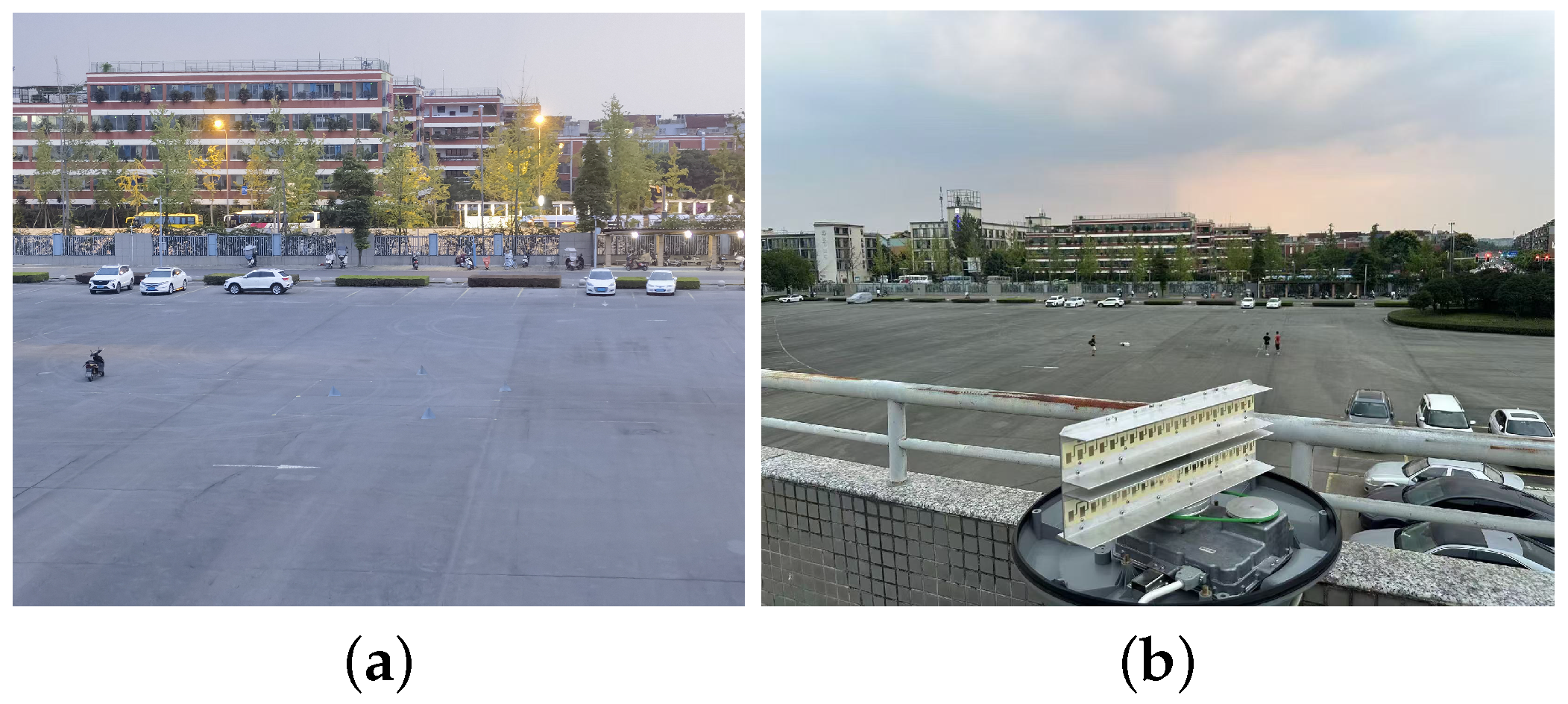
The experiment was conducted in the South Second Gate parking lot of the University of Electronic Science and Technology of China, Chengdu, China. The experimental scenario is shown in Figure 9a, where the distant area contains complex scenes such as houses, vehicles, and flowerbeds. The nearby area is relatively open, and we placed four corner reflectors within this space as sparse targets.

Meanwhile, the experiment employed an X-band radar, with the physical setup depicted in Figure 9b. The radar scans in a circular pattern with a certain downward angle, obtaining real beam result of the experiment.

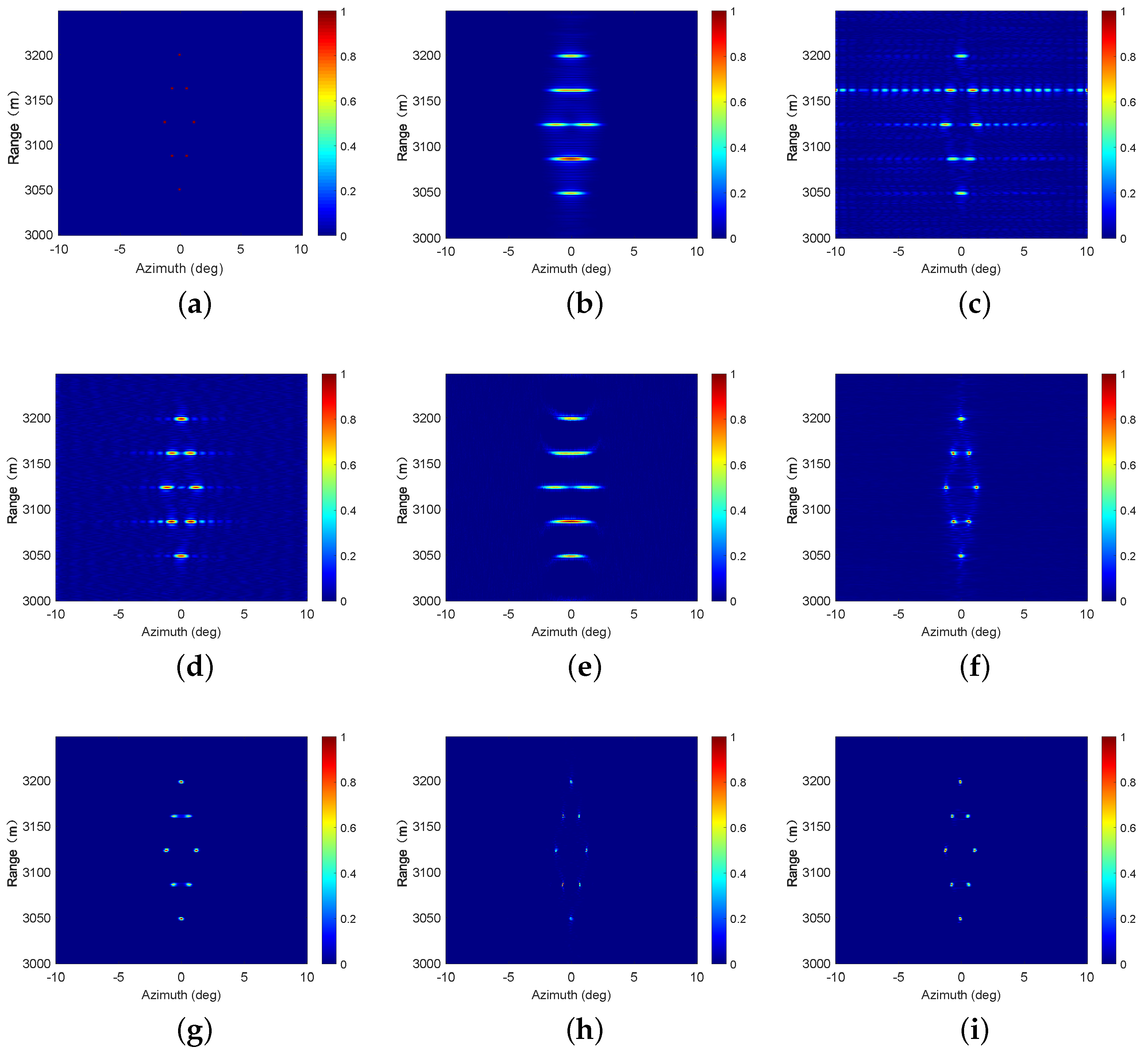
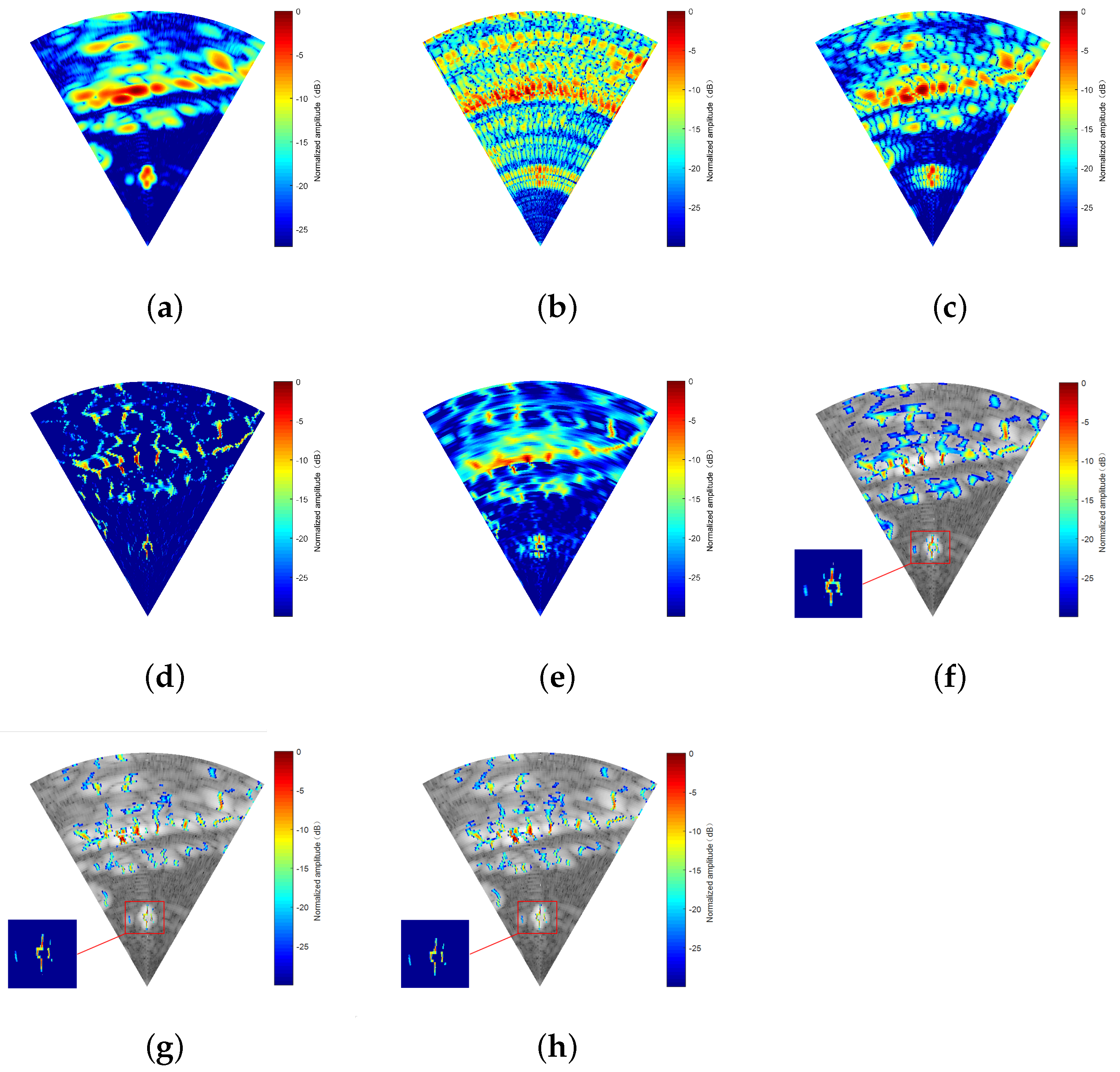
Figure 10 presentes the experimental results, with a matrix dimension of $129\times 171$ (range × azimuth). As presented in Figure 10a, the real beam echo in this region exhibits low resolution and high noise levels, making it almost difficult to discern targets. Figure 10b–h are the reconstructed target results after processing the real beam echoes using various algorithms. In Figure 10b, the TSVD method results in highly cluttered reconstructed targets due to its high side lobes. As shown in Figure 10c, the REGU algorithm exhibits a certain degree of side lobe suppression. The image quality is significantly enhanced compared to that obtained using the TSVD algorithm, although its resolution enhancement is still relatively limited. Figure 10d presents the results obtained using the Lucy method, which exhibits some suppression of side lobes. However, the lower resolution prevents it from obtaining a satisfactory image. Figure 10e is the result of the IAA algorithm, with an improved resolution enhancement. However, it fails to suppress the strong noise, and significant residual shadows are present in the image. In Figure 10f–h, to demonstrate the improvement achieved by the $L_1$-based methods, the real beam data are merged in the bottom layer. Figure 10f represents the result of the batch processing sparse $L_1$ regularization algorithm, which effectively distinguishes the sparse targets. But there is still some merging between the targets, as shown in the enlarged part. Figure 10g,h display the results of the online sparse $L_1$ regularization algorithm and the proposed algorithm, respectively. It can be observed that both algorithms exhibit a significant improvement in resolution. However, the online sparse $L_1$ regularization algorithm used to generate Figure 10g imposes a substantial computational burden due to its online structure, while the proposed algorithm used to generate Figure 10h effectively addresses this issue based on the LGBRT framework. Meanwhile, compared with the online sparse $L_1$ regularization algorithm, the ET of the proposed algorithm decreases from 185.62 s to 36.41 s.

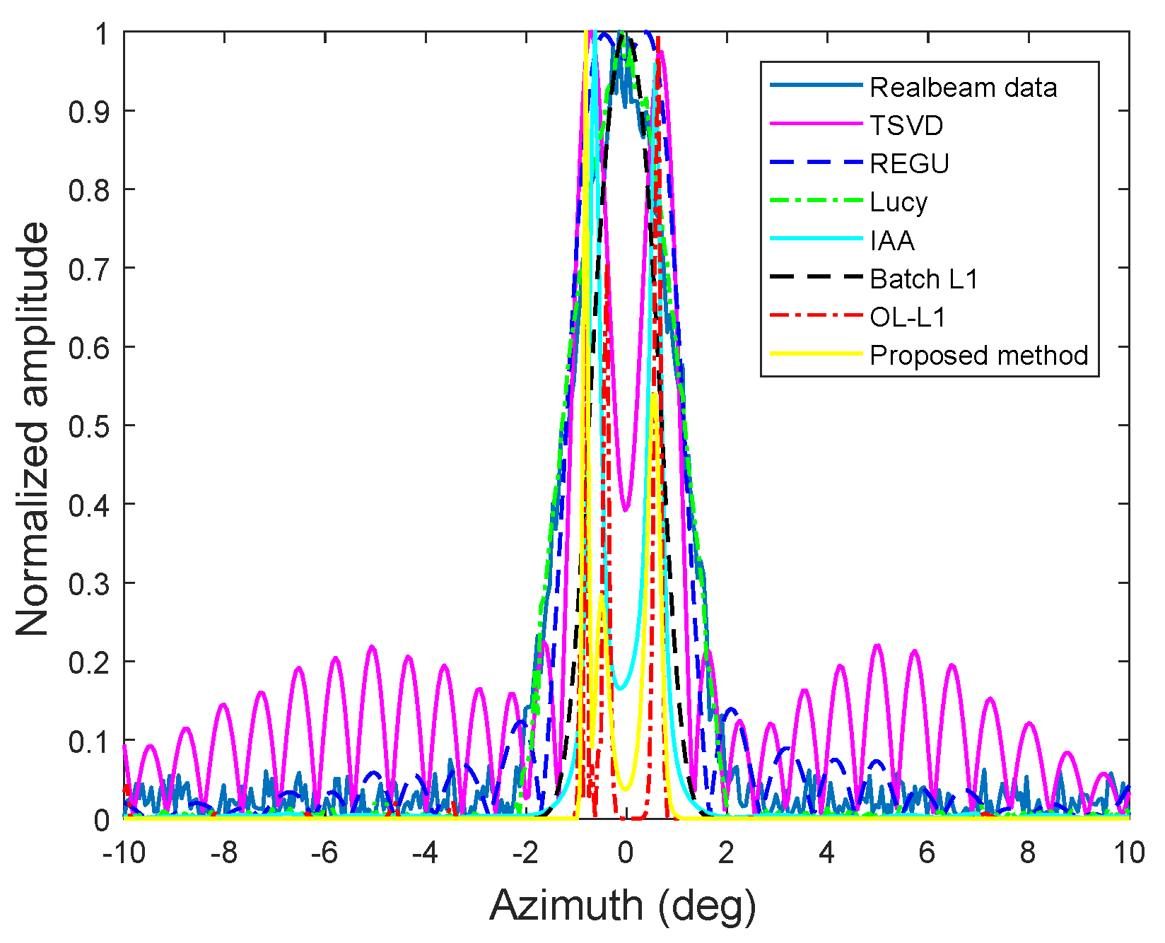
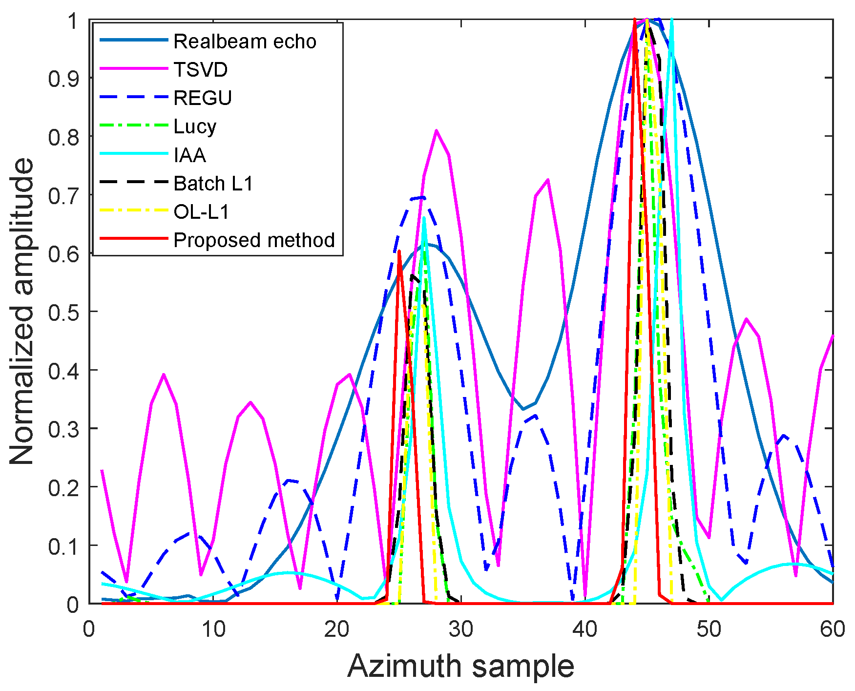
To further provide an intuitive comparison of the reconstruction performance across different algorithms, Figure 11 presents the profiles of the targets at a range of 27 m. It can be seen that the proposed algorithm not only successfully distinguishes the sparse targets but also has the narrowest beam width, undoubtedly demonstrating its outstanding reconstruction performance. Hence, the experimental data processing results also prove the effectiveness of the proposed method.

6. Conclusions

This paper introduces an online BRS-based updating framework aimed at improving computational efficiency and reducing storage requirements in target reconstruction for RAR. First, by incorporating sparse prior information into the regularization framework, the target reconstruction problem can be reformulated as an $L_1$-norm minimization issue. Then, an online structure of sparse $L_1$ regularization model is further proposed. Finally, based on the correspondence between echo pulse samples and target grids, the framework proposed in this article decomposes the global recursive updating of the complete echo region into local recursive updating of multiple unit echo regions, so it effectively achieves online fast target reconstruction.

To evaluate the effectiveness of the proposed algorithm, this paper presents the result simulation and experimental data which indicate that the proposed algorithm exhibits comparable target reconstruction performance to the online sparse $L_1$ regularization method. Consequently, the primary advantage of the proposed method lies in its approximately sixfold improvement in computational speed compared to the conventional online sparse $L_1$ regularization approach. Moreover, it enables real-time target reconstruction during beam scanning without incurring processor latency. However, the current derivation of this framework is limited to the online $L_1$ regularization algorithm, which somewhat restricts its generality. In future work, leveraging the inherent physical consistency of scanning radar systems, we aim to extend this framework into a more generalized version applicable to a wider range of target reconstruction algorithms.

References

1. Soldovieri, F.; Gennarelli, G.; Catapano, I.; Liao, D.; Dogaru, T. Forward-looking radar imaging: A comparison of two data processing strategies. IEEE J. Sel. Top. Appl. Earth Obs. Remote Sens. 2016, 10, 562–571. [Google Scholar] [CrossRef]
2. Zhang, Y.; Mao, D.; Zhang, Q.; Zhang, Y.; Huang, Y.; Yang, J. Airborne forward-looking radar super-resolution imaging using iterative adaptive approach. IEEE J. Sel. Top. Appl. Earth Obs. Remote Sens. 2019, 12, 2044–2054. [Google Scholar] [CrossRef]
3. Zhang, Q.; Zhang, Y.; Huang, Y.; Zhang, Y. Azimuth superresolution of forward-looking radar imaging which relies on linearized Bregman. IEEE J. Sel. Top. Appl. Earth Obs. Remote Sens. 2019, 12, 2032–2043. [Google Scholar] [CrossRef]
4. Yin, X.; Zhang, Y.; Mao, D.; Zhang, Y.; Huang, Y.; Yang, J. A Parameter-Free Estimation Method Based on Low-Rank and Sparse Hybrid Constraints for Scanning Radar Forward-Looking Imaging. In Proceedings of the IGARSS 2024-2024 IEEE International Geoscience and Remote Sensing Symposium, Athens, Greece, 7–12 July 2024; IEEE: Piscataway, NJ, USA, 2024; pp. 10524–10528. [Google Scholar]
5. Chen, H.; Li, M.; Zhang, P.; Liu, G.; Jia, L.; Wu, Y. Resolution enhancement for Doppler beam sharpening imaging. IET Radar Sonar Navig. 2015, 9, 843–851. [Google Scholar] [CrossRef]
6. Moreira, A.; Huang, Y. Airborne SAR processing of highly squinted data using a chirp scaling approach with integrated motion compensation. IEEE Trans. Geosci. Remote Sens. 1994, 32, 1029–1040. [Google Scholar] [CrossRef]
7. Richards, M.A. Iterative noncoherent angular superresolution (radar). In Proceedings of the 1988 IEEE National Radar Conference, Ann Arbor, MI, USA, 20–21 April 1988; IEEE: Piscataway, NJ, USA, 1988; pp. 100–105. [Google Scholar]
8. Uttam, S.; Goodman, N.A. Superresolution of coherent sources in real-beam data. IEEE Trans. Aerosp. Electron. Syst. 2010, 46, 1557–1566. [Google Scholar] [CrossRef]
9. Mao, D.; Yang, J.; Zhang, Y.; Huo, W.; Xu, F.; Pei, J.; Zhang, Y.; Huang, Y. Angular superresolution of real aperture radar with high-dimensional data: Normalized projection array model and adaptive reconstruction. IEEE Trans. Geosci. Remote Sens. 2022, 60, 5117216. [Google Scholar] [CrossRef]
10. Zrnic, D.; Doviak, R. Effective antenna pattern of scanning radars. IEEE Trans. Aerosp. Electron. Syst. 1976, AES-12, 551–555. [Google Scholar] [CrossRef]
11. Heron, M.; Gill, E.; Prytz, A. An investigation of double-peaked HF radar spectra via a convolution/de-convolution algorithm. In Proceedings of the OCEANS 2008-MTS/IEEE Kobe Techno-Ocean, Kobe, Japan, 8–11 April 2008; IEEE: Piscataway, NJ, USA, 2008; pp. 1–5. [Google Scholar]
12. Shen, J.; Zhang, Y.; Mao, D.; Huang, Y.; Yang, J. Extended Target Reconstruction for Real Aperture Radar Using Sparse and Two-dimensional High-order Gradient Hybrid Prior Bayesian Method. IEEE Trans. Geosci. Remote. Sens. 2025, 63, 5103814. [Google Scholar] [CrossRef]
13. Guan, J.; Yang, J.; Huang, Y.; Li, W. Maximum a posteriori–based angular superresolution for scanning radar imaging. IEEE Trans. Aerosp. Electron. Syst. 2014, 50, 2389–2398. [Google Scholar] [CrossRef]
14. Zha, Y.; Huang, Y.; Sun, Z.; Wang, Y.; Yang, J. Bayesian deconvolution for angular super-resolution in forward-looking scanning radar. Sensors 2015, 15, 6924–6946. [Google Scholar] [CrossRef] [PubMed]
15. Chen, H.; Li, Y.; Gao, W.; Zhang, W.; Sun, H.; Guo, L.; Yu, J. Bayesian forward-looking superresolution imaging using Doppler deconvolution in expanded beam space for high-speed platform. IEEE Trans. Geosci. Remote Sens. 2021, 60, 5105113. [Google Scholar] [CrossRef]
16. Guo, Y.; Liang, Y.; Liang, Y.; Sun, X. Structured Bayesian Super-Resolution Forward-Looking Imaging for Maneuvering Platforms Based on Enhanced Sparsity Model. Remote Sens. 2025, 17, 775. [Google Scholar] [CrossRef]
17. Shea, J.D.; Van Veen, B.D.; Hagness, S.C. A TSVD analysis of microwave inverse scattering for breast imaging. IEEE Trans. Biomed. Eng. 2011, 59, 936–945. [Google Scholar] [CrossRef]
18. Lenti, F.; Nunziata, F.; Migliaccio, M.; Rodriguez, G. Two-dimensional TSVD to enhance the spatial resolution of radiometer data. IEEE Trans. Geosci. Remote Sens. 2013, 52, 2450–2458. [Google Scholar] [CrossRef]
19. Tuo, X.; Zhang, Y.; Huang, Y.; Yang, J. Fast sparse-TSVD super-resolution method of real aperture radar forward-looking imaging. IEEE Trans. Geosci. Remote Sens. 2020, 59, 6609–6620. [Google Scholar] [CrossRef]
20. Gambardella, A.; Migliaccio, M. On the superresolution of microwave scanning radiometer measurements. IEEE Geosci. Remote Sens. Lett. 2008, 5, 796–800. [Google Scholar] [CrossRef]
21. Anandan, V.; Reddy, G.R.; Rao, P. Spectral analysis of atmospheric radar signal using higher order spectral estimation technique. IEEE Trans. Geosci. Remote Sens. 2001, 39, 1890–1895. [Google Scholar] [CrossRef]
22. Álvarez-Pérez, J.L.; Marshall, S.J.; Gregson, K. Resolution improvement of ERS scatterometer data over land by Wiener filtering. Remote Sens. Environ. 2000, 71, 261–271. [Google Scholar] [CrossRef]
23. Van der Baan, M. Bandwidth enhancement: Inverse Q filtering or time-varying Wiener deconvolution? Geophysics 2012, 77, V133–V142. [Google Scholar] [CrossRef]
24. Yardibi, T.; Li, J.; Stoica, P.; Xue, M.; Baggeroer, A.B. Source localization and sensing: A nonparametric iterative adaptive approach based on weighted least squares. IEEE Trans. Aerosp. Electron. Syst. 2010, 46, 425–443. [Google Scholar] [CrossRef]
25. Zhang, Y.; Li, W.; Zhang, Y.; Huang, Y.; Yang, J. A fast iterative adaptive approach for scanning radar angular superresolution. IEEE J. Sel. Top. Appl. Earth Obs. Remote Sens. 2015, 8, 5336–5345. [Google Scholar] [CrossRef]
26. Zhang, Y.; Jakobsson, A.; Yang, J. Range-recursive IAA for scanning radar angular super-resolution. IEEE Geosci. Remote Sens. Lett. 2017, 14, 1675–1679. [Google Scholar] [CrossRef]
27. Candes, E.J.; Romberg, J.K.; Tao, T. Stable signal recovery from incomplete and inaccurate measurements. Commun. Pure Appl. Math. A J. Issued Courant Inst. Math. Sci. 2006, 59, 1207–1223. [Google Scholar] [CrossRef]
28. Candès, E.J.; Romberg, J.; Tao, T. Robust uncertainty principles: Exact signal reconstruction from highly incomplete frequency information. IEEE Trans. Inf. Theory 2006, 52, 489–509. [Google Scholar] [CrossRef]
29. Candès, E.J.; Wakin, M.B. An introduction to compressive sampling. IEEE Signal Process. Mag. 2008, 25, 21–30. [Google Scholar] [CrossRef]
30. Herman, M.A.; Strohmer, T. High-resolution radar via compressed sensing. IEEE Trans. Signal Process. 2009, 57, 2275–2284. [Google Scholar] [CrossRef]
31. Potter, L.C.; Ertin, E.; Parker, J.T.; Cetin, M. Sparsity and compressed sensing in radar imaging. Proc. IEEE 2010, 98, 1006–1020. [Google Scholar] [CrossRef]
32. Tourbier, S.; Bresson, X.; Hagmann, P.; Thiran, J.P.; Meuli, R.; Cuadra, M.B. An efficient total variation algorithm for super-resolution in fetal brain MRI with adaptive regularization. NeuroImage 2015, 118, 584–597. [Google Scholar] [CrossRef]
33. Jiang, J.; Chen, C.; Huang, K.; Cai, Z.; Hu, R. Noise robust position-patch based face super-resolution via Tikhonov regularized neighbor representation. Inf. Sci. 2016, 367, 354–372. [Google Scholar] [CrossRef]
34. Wright, J.; Yang, A.Y.; Ganesh, A.; Sastry, S.S.; Ma, Y. Robust face recognition via sparse representation. IEEE Trans. Pattern Anal. Mach. Intell. 2008, 31, 210–227. [Google Scholar] [CrossRef] [PubMed]
35. Yang, J.; Wright, J.; Huang, T.S.; Ma, Y. Image super-resolution via sparse representation. IEEE Trans. Image Process. 2010, 19, 2861–2873. [Google Scholar] [CrossRef] [PubMed]
36. Chartrand, R.; Yin, W. Iteratively reweighted algorithms for compressive sensing. In Proceedings of the 2008 IEEE International Conference on Acoustics, Speech and Signal Processing, Las Vegas, NV, USA, 31 March–4 April 2008; IEEE: Piscataway, NJ, USA, 2008; pp. 3869–3872. [Google Scholar]
37. Wang, J.; Ma, J.; Han, B.; Li, Q. Split Bregman iterative algorithm for sparse reconstruction of electrical impedance tomography. Signal Process. 2012, 92, 2952–2961. [Google Scholar] [CrossRef]
38. Xiong, K.; Zhao, G.; Shi, G.; Wang, Y. A convex optimization algorithm for compressed sensing in a complex domain: The complex-valued split Bregman method. Sensors 2019, 19, 4540. [Google Scholar] [CrossRef]
39. Bayram, I.; Selesnick, I.W. A subband adaptive iterative shrinkage/thresholding algorithm. IEEE Trans. Signal Process. 2009, 58, 1131–1143. [Google Scholar] [CrossRef]
40. Zha, Y.; Huang, Y.; Yang, J. Augmented Lagrangian method for angular super-resolution imaging in forward-looking scanning radar. J. Appl. Remote Sens. 2015, 9, 096055. [Google Scholar] [CrossRef]
41. Sriperumbudur, B.K.; Torres, D.A.; Lanckriet, G.R. A majorization-minimization approach to the sparse generalized eigenvalue problem. Mach. Learn. 2011, 85, 3–39. [Google Scholar] [CrossRef]
42. Sun, Y.; Babu, P.; Palomar, D.P. Majorization-minimization algorithms in signal processing, communications, and machine learning. IEEE Trans. Signal Process. 2016, 65, 794–816. [Google Scholar] [CrossRef]
43. Yin, X.; Huang, Y.; Zhang, Y.; Zhang, Y.; Tuo, X.; Zhang, Y.; Yang, J. Online Sparse Super-Resolution Method for Radar Forward-Looking Imaging Using Majorize-Minimization. In Proceedings of the IGARSS 2023-2023 IEEE International Geoscience and Remote Sensing Symposium, Pasadena, CA, USA, 16–21 July 2023; IEEE: Piscataway, NJ, USA, 2023; pp. 7129–7132. [Google Scholar]
44. Mukherjee, S.; Chen, H.; Veeraraghavan, A.; Seelamantula, C.S. Online Reweighted Least Squares Algorithm for Sparse Recovery and Application to Short-Wave Infrared Imaging. arXiv 2017, arXiv:1706.09585. [Google Scholar]
45. Gill, P.E.; Murray, W. Algorithms for the solution of the nonlinear least-squares problem. SIAM J. Numer. Anal. 1978, 15, 977–992. [Google Scholar] [CrossRef]
46. Swärd, J.; Adalbjörnsson, S.I.; Jakobsson, A. Generalized sparse covariance-based estimation. Signal Process. 2018, 143, 311–319. [Google Scholar] [CrossRef]
47. Zhang, Q.; Zhang, Y.; Huang, Y.; Zhang, Y.; Li, W.; Yang, J. Sparse with fast MM superresolution algorithm for radar forward-looking imaging. IEEE Access 2019, 7, 105247–105257. [Google Scholar] [CrossRef]
48. Tuo, X.; Zhang, Y.; Huang, Y.; Yang, J. A fast sparse azimuth super-resolution imaging method of real aperture radar based on iterative reweighted least squares with linear sketching. IEEE J. Sel. Top. Appl. Earth Obs. Remote Sens. 2021, 14, 2928–2941. [Google Scholar] [CrossRef]
49. Akgün, M.A.; Garcelon, J.H.; Haftka, R.T. Fast exact linear and non-linear structural reanalysis and the Sherman–Morrison–Woodbury formulas. Int. J. Numer. Methods Eng. 2001, 50, 1587–1606. [Google Scholar] [CrossRef]
Figure 1. (a) Top-view schematic diagram of the airborne RAR imaging model (b) Side-view schematic diagram of the airborne RAR imaging model.
Remotesensing 17 01887 g001
Figure 2. Correspondence between echo pulse samples and target grids.
Remotesensing 17 01887 g002
Figure 3. Local updating framework within unit echo region.
Remotesensing 17 01887 g003
Figure 4. Flowchart of the proposed algorithm.
Remotesensing 17 01887 g004
Figure 5. The antenna pattern for simulations.
Remotesensing 17 01887 g005
Figure 6. Results of 1D point simulation. (a) Initial scene; (b) real beam echo; (c) the TSVD algorithm result; (d) the REGU algorithm result; (e) the Lucy algorithm result; (f) the IAA algorithm result; (g) the batch processing sparse L 1 regularization algorithm result; (h) the online sparse L 1 regularization algorithm result; (i) the proposed algorithm result.
Remotesensing 17 01887 g006
Figure 7. Results of 2D area simulation. (a) Initial scene; (b) real beam echo; (c) the TSVD algorithm result; (d) the REGU algorithm result; (e) the Lucy algorithm result; (f) the IAA algorithm result; (g) the batch processing sparse L 1 regularization algorithm result; (h) the online sparse L 1 regularization algorithm result; (i) the proposed algorithm result.
Remotesensing 17 01887 g007
Figure 8. Profile results for adjacent targets located at a distance of 3161 m.
Remotesensing 17 01887 g008
Figure 9. (a) Optical experimental scene. (b) RAR system used in the experiment.
Remotesensing 17 01887 g009
Figure 10. Results of experimental datas. (a) Real beam echo; (b) the TSVD algorithm result; (c) the REGU algorithm result; (d) the Lucy algorithm result; (e) the IAA algorithm result; (f) the batch processing sparse L 1 regularization algorithm result; (g) the online sparse L 1 regularization algorithm result; (h) the proposed algorithm result.
Remotesensing 17 01887 g010
Figure 11. The profiles of the targets within the red rectangle above.
Remotesensing 17 01887 g011