
OGAIS: OpenGL-Driven GPU Acceleration Methodology for 3D Hyperspectral Image Simulation


Abstract

1. Introduction
2. Simulation Model
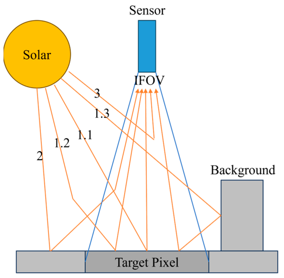
2.1. Radiative Transfer
2.2. Ray Tracing Algorithm
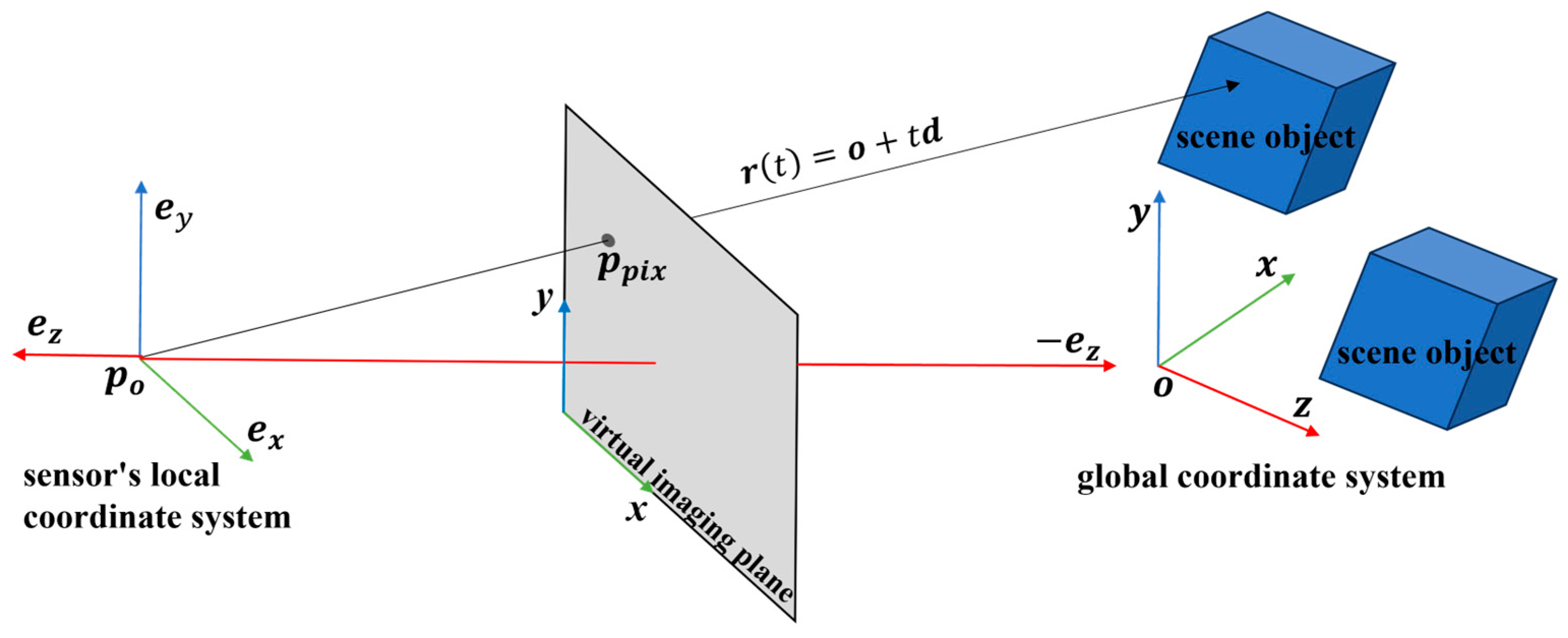
2.2.1. Sensor-Originated Ray Casting
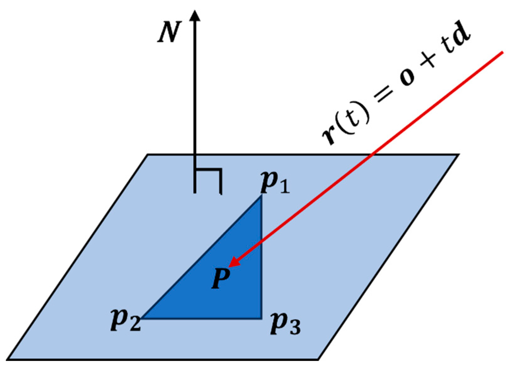
2.2.2. Ray-Scene Intersection Calculation
2.2.3. Radiation Calculation
3. Implementation and Acceleration
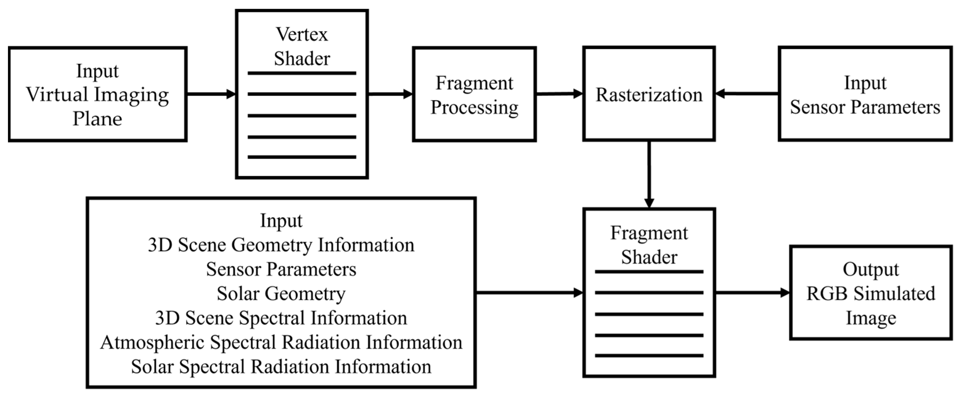
3.1. Implementation of Model Based on OpenGL
3.1.1. Implementation of RGB Ray Tracing
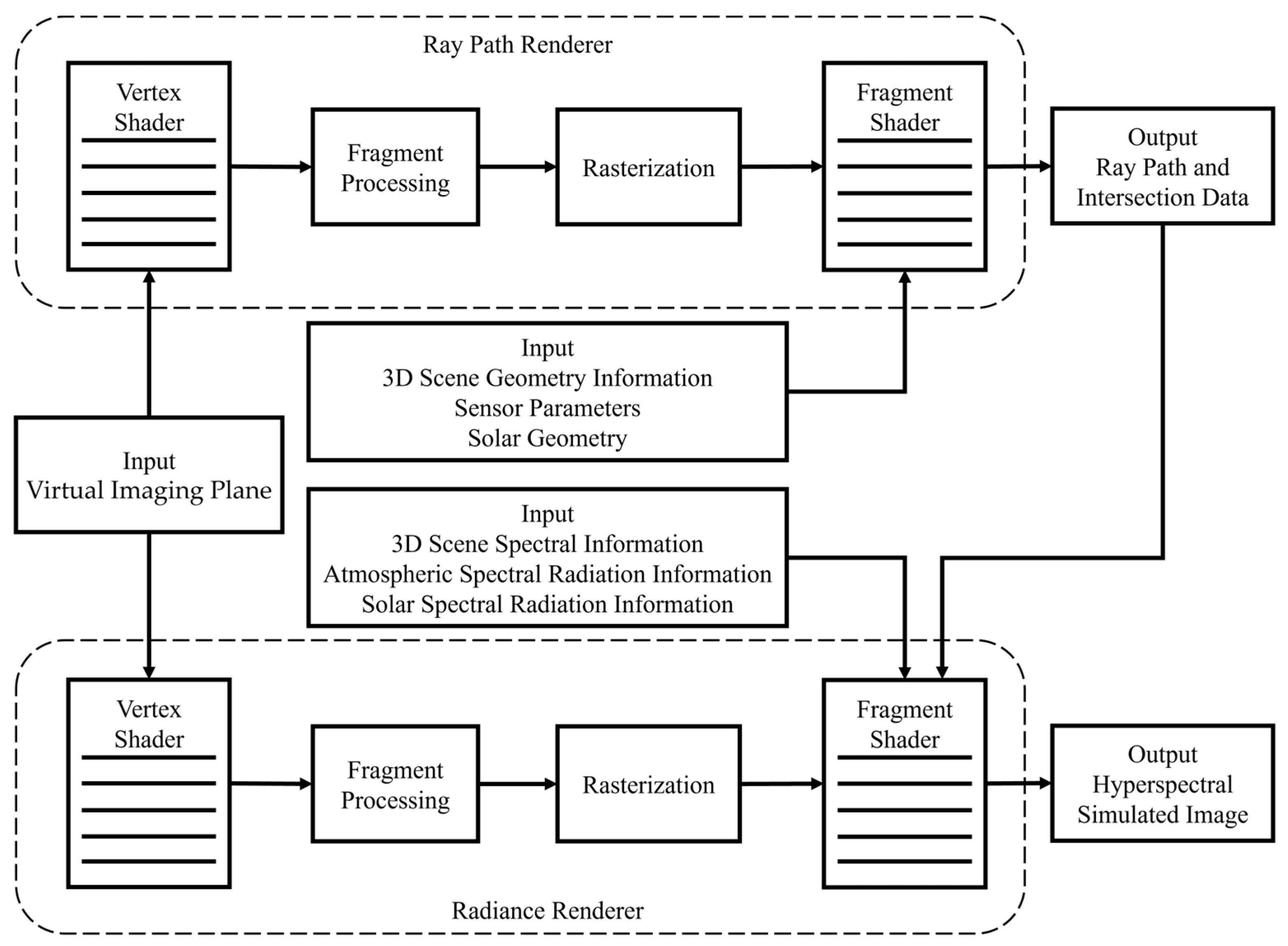
3.1.2. Implementation of Hyperspectral Ray Tracing
| Algorithm 1 TraditionalRayTracing | |
| 1: | InitializeRayTracingRenderer(vertex_shader, fragment_shader) |
| 2: | InputParameters(scene_geometry, sensor_params, solar_geometry, |
| 3: | scene_spectral_data, atmospheric_radiation, solar_radiation) |
| 4: | for each band: |
| 5: | for each ray: |
| 6: | Calculate ray path and radiance → single_band_single_ray_image |
| 7: | Store in single_band_multi_ray_image |
| 8: | end for |
| 9: | Store single_band_multi_ray_image in multi_band_image |
| 10: | end for |
| Algorithm 2 ModifiedRayTracing | |
| 11: | InitializeRayPathRenderer(vertex_shader, path_calculation_shader) |
| 12: | InputParameters(scene_geometry, sensor_params, solar_geometry) |
| 13: | for each ray: |
| 14: | Calculate ray path → single_ray_data |
| 15: | Store in multi_ray_data |
| 16: | end for |
| 17: | InitializeRadianceRenderer(vertex_shader, radiance_calculation_shader) |
| 18: | InputParameters(multi_ray_data, scene_spectral_data, |
| 19: | atmospheric_radiation, solar_radiation) |
| 20: | for each band: |
| 21: | Calculate radiance → single_band_multi_ray_image |
| 22: | Store in multi_band_image |
| 23: | end for |
3.1.3. Efficiency Verification of the Simulation
3.2. Model Acceleration
3.2.1. Accelerate at the Algorithmic Level
- (1)
- Compute the bounding box of the current node
- (2)
- Select the optimal splitting axis (typically via SAH* evaluation)
- (3)
- Determine the splitting plane position
- (4)
- Generate left/right child nodes
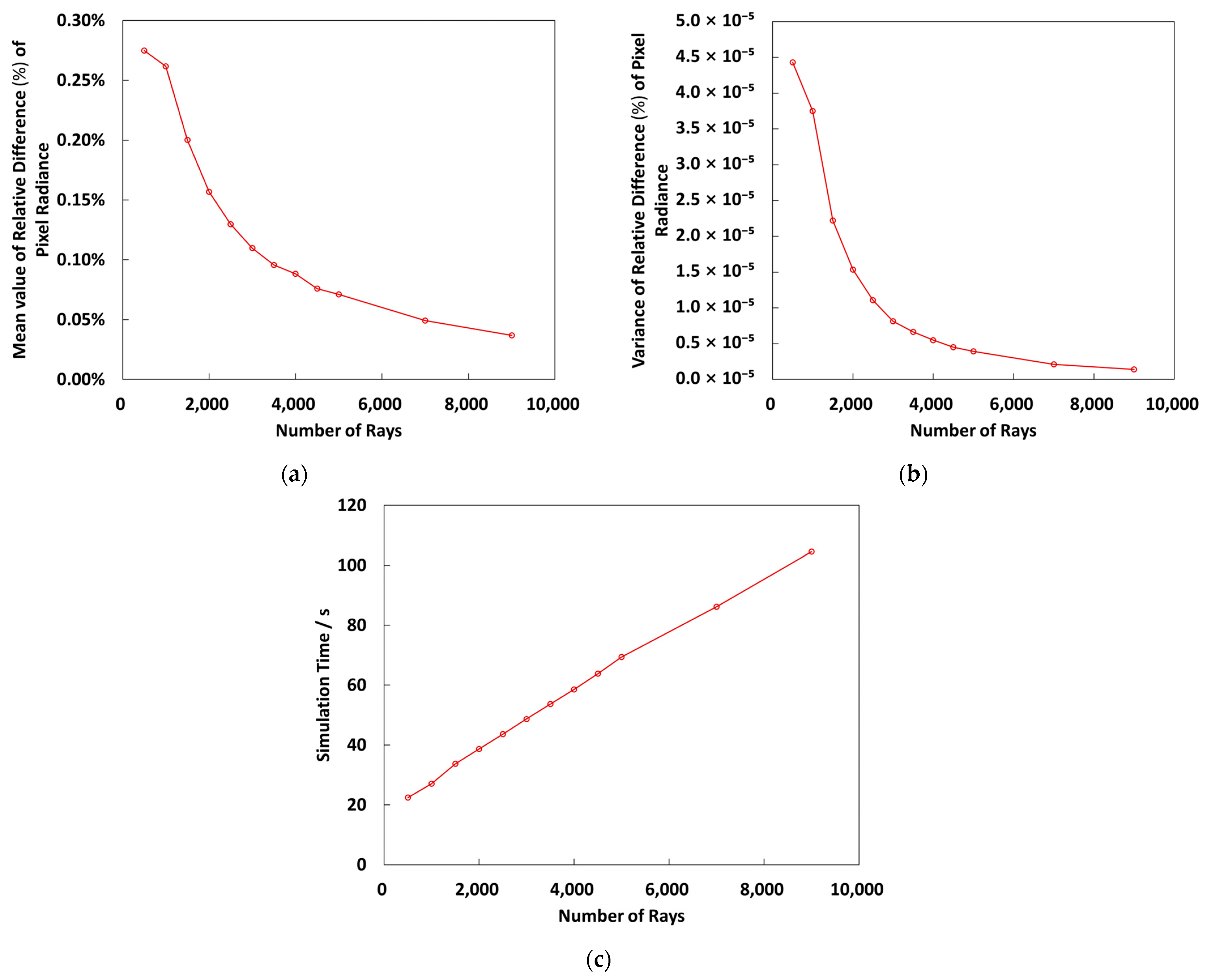
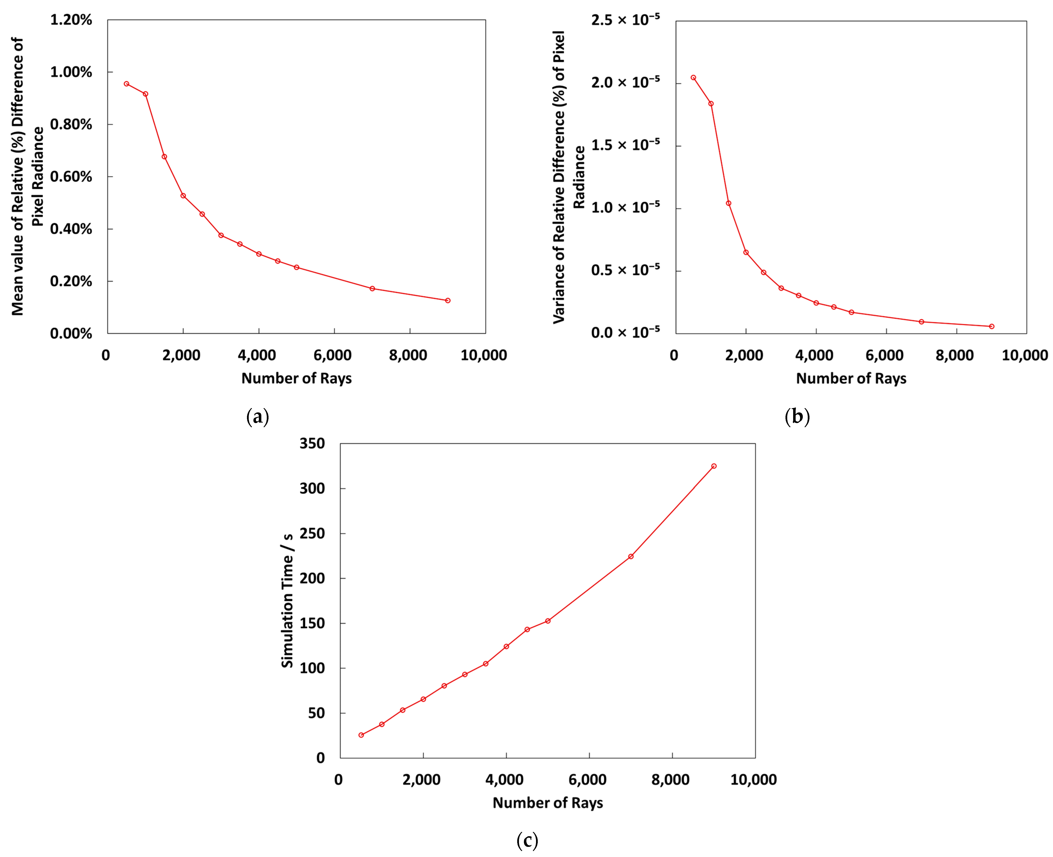
3.2.2. Explore the Balance Between Accuracy and Efficiency
4. UAV-Based Data Validation
4.1. Acquisition of UAV Data
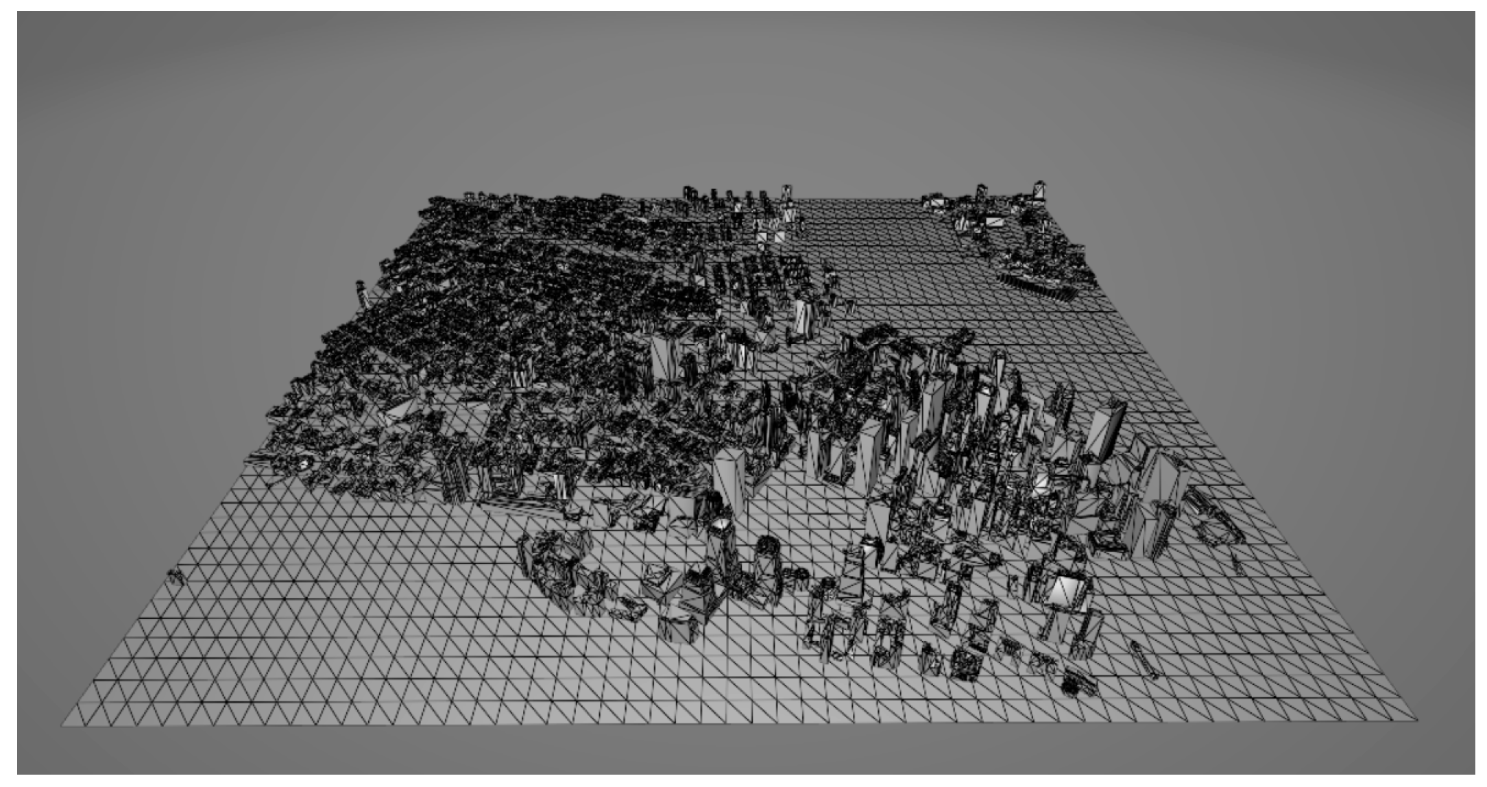
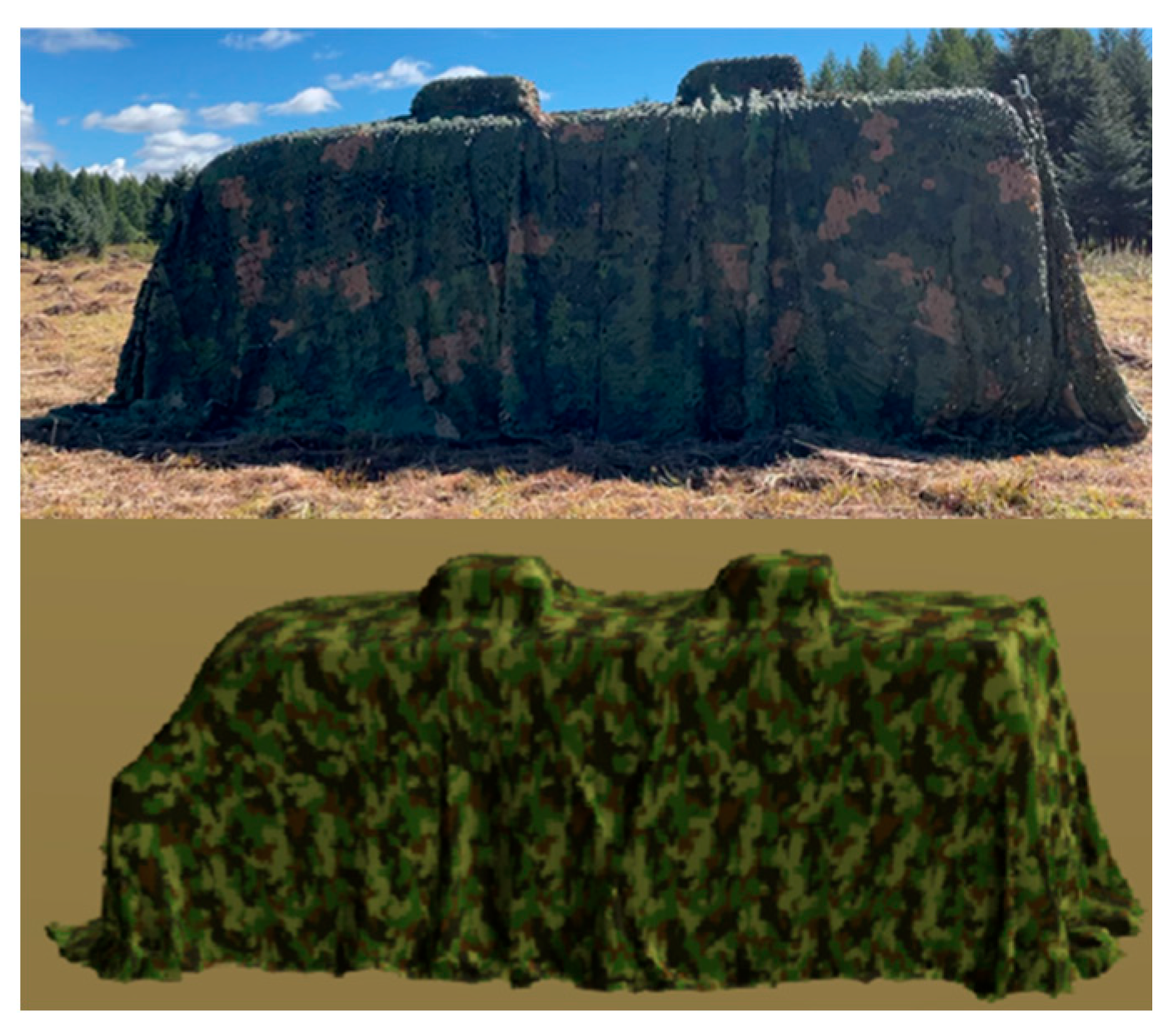
4.2. 3D Model Construction
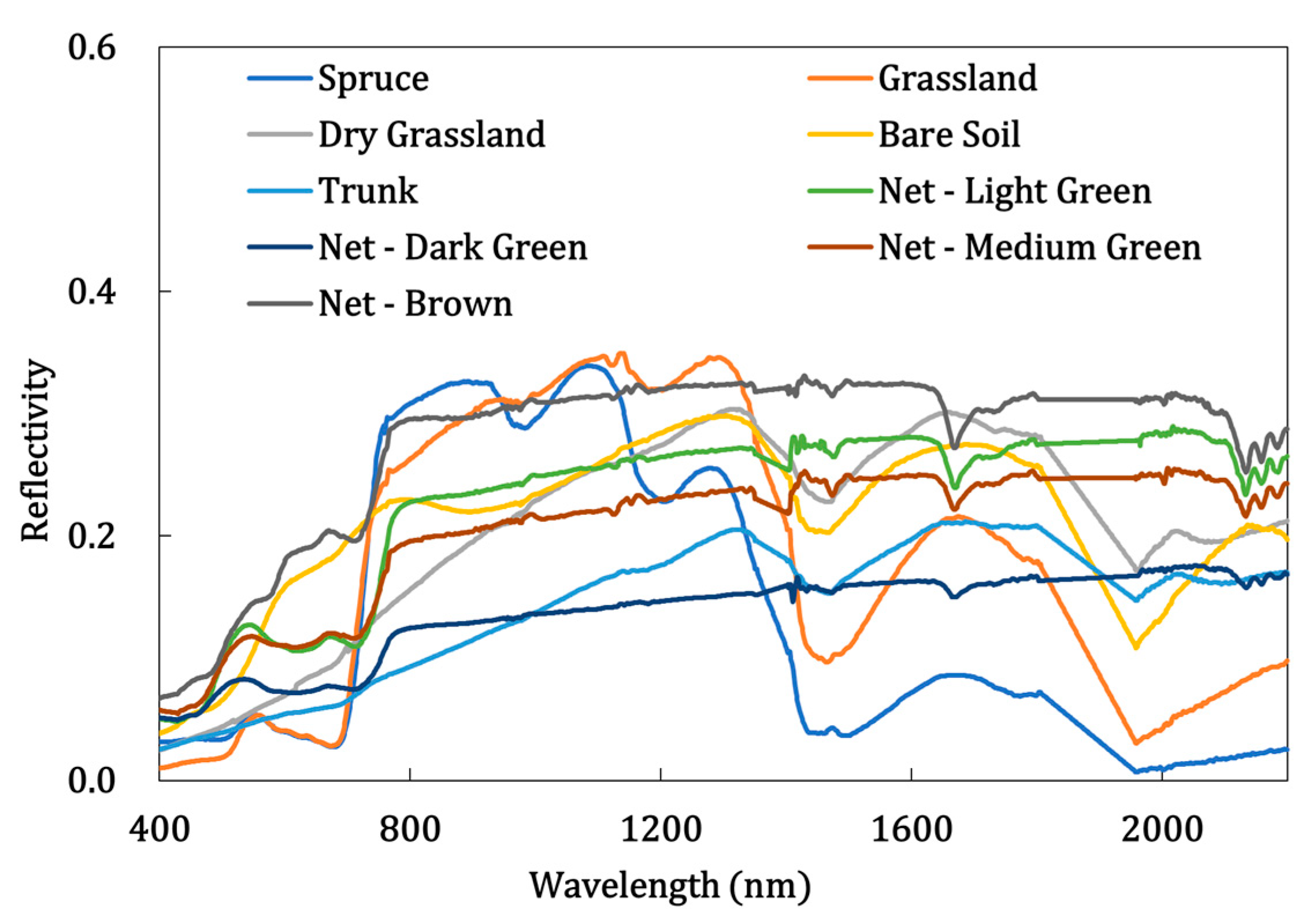
4.3. Reflectance Data Acquisition
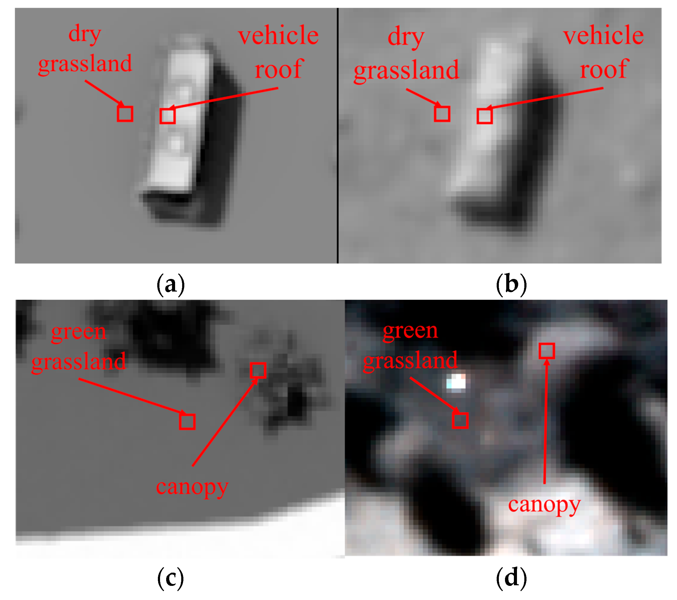
4.4. Validation Results
5. Discussion
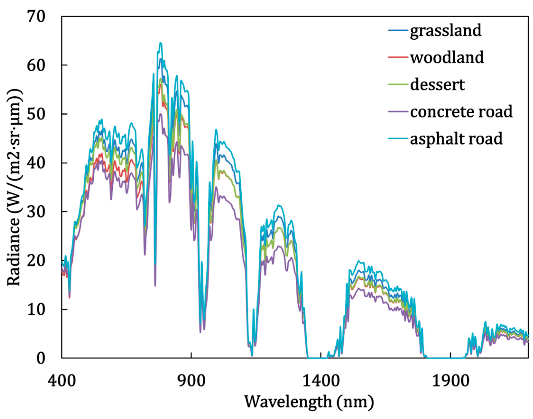
5.1. Effect of Background on Spectral Radiance
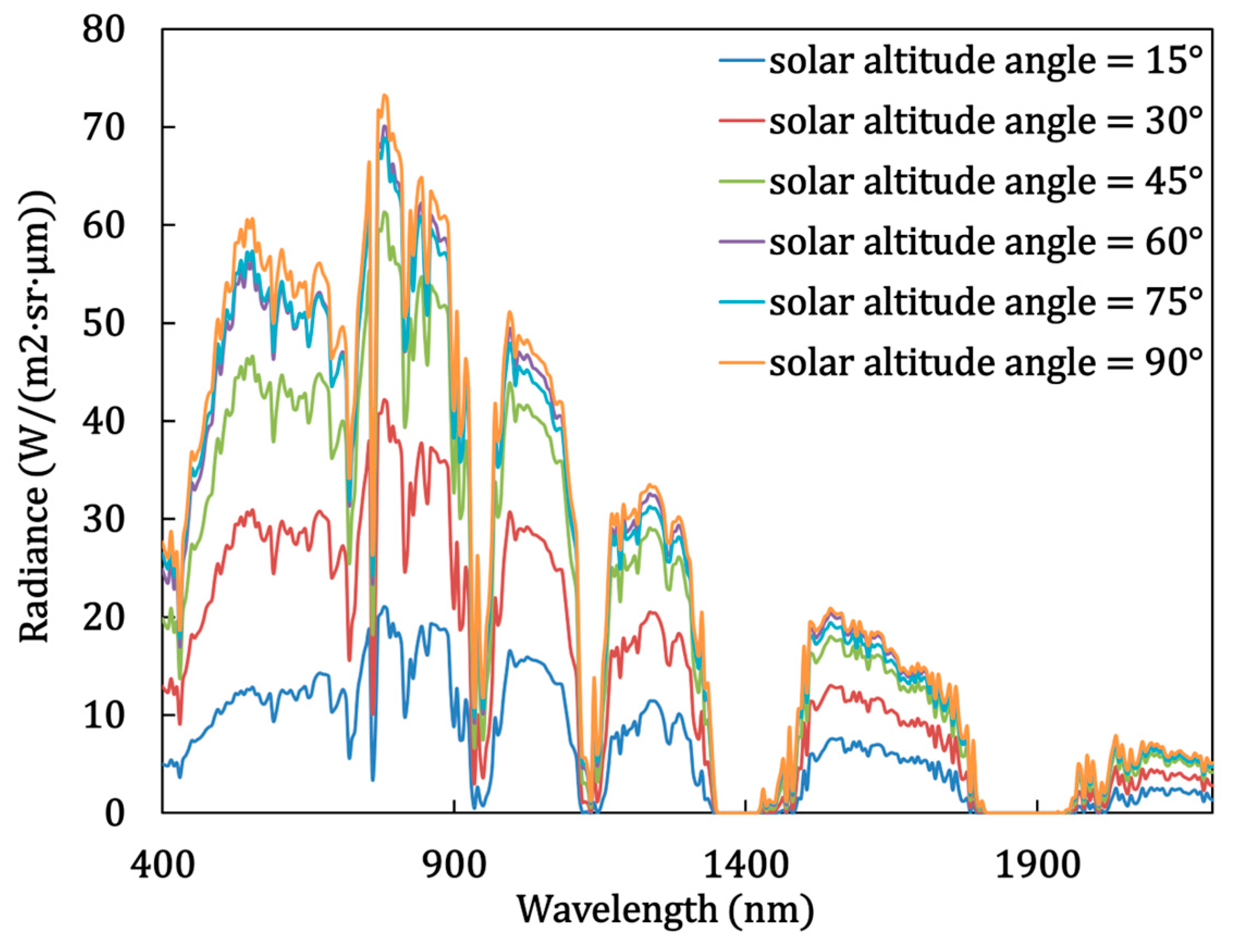
5.2. Effect of Solar Altitude Angle on Spectral Radiances
5.3. Effect of Sensor Altitude Angle on Spectral Radiance
5.4. Section Summary
6. Conclusions
Author Contributions
Funding
Data Availability Statement
Conflicts of Interest
References
- Goetz, A.F.; Vane, G.; Solomon, J.E.; Rock, B.N. Imaging spectrometry for Earth remote sensing. Science 1985, 228, 1147–1153. [Google Scholar] [CrossRef]
- Lu, B.; Dao, P.D.; Liu, J.; He, Y.; Shang, J. Recent Advances of Hyperspectral Imaging Technology and Applications in Agriculture. Remote Sens. 2020, 12, 2659. [Google Scholar] [CrossRef]
- Liu, B.; Tong, Q.X.; Zhang, L.F.; Zhang, X.; Yue, Y.M.; Zhang, B. Monitoring Spatio-Temporal Spectral Characteristics of Leaves of Karst Plant during Dehydration Using a Field Imaging Spectrometer System. Spectrosc. Spectr. Anal. 2012, 32, 1460–1465. [Google Scholar] [CrossRef]
- Shi, T.; Chen, Y.; Liu, Y.; Wu, G. Visible and near-infrared reflectance spectroscopy-An alternative for monitoring soil contamination by heavy metals. J. Hazard. Mater. 2014, 265, 166–176. [Google Scholar] [CrossRef]
- Liang, L.; Di, L.; Zhang, L.; Deng, M.; Qin, Z.; Zhao, S.; Lin, H. Estimation of crop LAI using hyperspectral vegetation indices and a hybrid inversion method. Remote Sens. Environ. 2015, 165, 123–134. [Google Scholar] [CrossRef]
- Goetz, A.F.H. Three decades of hyperspectral remote sensing of the Earth: A personal view. Remote Sens. Environ. 2009, 113, S5–S16. [Google Scholar] [CrossRef]
- Shimoni, M.; Haelterman, R.; Perneel, C. Hyperspectral Imaging for Military and Security Applications Combining myriad processing and sensing techniques. IEEE Geosci. Remote Sens. Mag. 2019, 7, 101–117. [Google Scholar] [CrossRef]
- Tang, G. Research on Visible Hyperspectral Imaging of Ground Sea Target (Chinese). Master’s Thesis, Xidian University, Xi’an, China, 2021. [Google Scholar]
- Zhang, B.; Chen, Z.C.; Zheng, L.F.; Tong, Q.X.; Liu, Y.N.; Yang, Y.D.; Xue, Y.Q. Object detection based on feature extraction from hyperspectral imagery and convex cone projection transform. J. Infrared Millim. Waves 2004, 23, 441–445+450. [Google Scholar]
- Lapadatu, M.; Bakken, S.; Grotte, M.E.; Alver, M.; Johansen, T.A. Simulation Tool for Hyper-Spectral Imaging From a Satellite. In Proceedings of the 2019 10th Workshop on Hyperspectral Imaging and Signal Processing: Evolution in Remote Sensing (WHISPERS), Amsterdam, The Netherlands, 24–26 September 2019; p. 5. [Google Scholar] [CrossRef]
- Zhao, S.; Zhu, X.; Tan, X.; Tian, J. Spectrotemporal fusion: Generation of frequent hyperspectral satellite imagery. Remote Sens. Environ. 2025, 319, 114639. [Google Scholar] [CrossRef]
- Li, J.; Zheng, K.; Gao, L.; Ni, L.; Huang, M.; Chanussot, J. Model-Informed Multistage Unsupervised Network for Hyperspectral Image Super-Resolution. IEEE Trans. Geosci. Remote Sens. 2024, 62, 3391014. [Google Scholar] [CrossRef]
- Cao, Y.; Cao, Y.; Wu, Z.; Yang, K. A Calculation Method for the Hyperspectral Imaging of Targets Utilizing a Ray-Tracing Algorithm. Remote Sens. 2024, 16, 1779. [Google Scholar] [CrossRef]
- Goodenough, A.A.; Brown, S.D. DIRSIG5: Next-Generation Remote Sensing Data and Image Simulation Framework. IEEE J. Sel. Top. Appl. Earth Obs. Remote Sens. 2017, 10, 4818–4833. [Google Scholar] [CrossRef]
- Wang, Y.; Kallel, A.; Zhen, Z.; Lauret, N.; Guilleux, J.; Chavanon, E.; Gastellu-Etchegorry, J.-P. 3D Monte Carlo differentiable radiative transfer with DART. Remote Sens. Environ. 2024, 308, 114201. [Google Scholar] [CrossRef]
- Qi, J.; Xie, D.; Yin, T.; Yan, G.; Gastellu-Etchegorry, J.-P.; Li, L.; Zhang, W.; Mu, X.; Norford, L.K. LESS: LargE-Scale remote sensing data and image simulation framework over heterogeneous 3D scenes. Remote Sens. Environ. 2019, 221, 695–706. [Google Scholar] [CrossRef]
- Gastellu-Etchegorry, J.-P.; Lauret, N.; Yin, T.; Landier, L.; Kallel, A.; Malenovsky, Z.; Al Bitar, A.; Aval, J.; Benhmida, S.; Qi, J.; et al. DART: Recent Advances in Remote Sensing Data Modeling With Atmosphere, Polarization, and Chlorophyll Fluorescence. IEEE J. Sel. Top. Appl. Earth Obs. Remote Sens. 2017, 10, 2640–2649. [Google Scholar] [CrossRef]
- Han, Y.; Lin, L.; Sun, H.; Jiang, J.; He, X. Modeling the space-based optical imaging of complex space target based on the pixel method. Optik 2015, 126, 1474–1478. [Google Scholar] [CrossRef]
- Han, Y.; Chen, M.; Sun, H.; Zhang, Y.; Kong, J. Imaging simulation method of TG-02 accompanying satellite’s visible camera. Infrared Laser Eng. 2017, 46, 1218002. [Google Scholar] [CrossRef]
- Chenfei, Y.; Hao, Z.; Guofeng, Z. Research on infrared imaging simulation technology of ocean scene. Proc. SPIE 2021, 12065, 1206513. [Google Scholar] [CrossRef]
- Xin, Y.; Yan, Z.; Xiao-Tian, C.; Feng, Z.; Jun-Jun, Z. An Infrared Radiation Simulation Method for Aircraft Target and Typical Ground Objects Based on RadThermIR and OpenGL. In Proceedings of the 2016 International Conference on Information Systems and Artificial Intelligence (ISAI), Hong Kong, China, 24–26 June 2016; pp. 236–240. [Google Scholar] [CrossRef]
- Jiang, W.; Zhao, Y.; Yuan, S. Modeling and OpenGL simulation of sea surface infrared images. Electron. Opt. Control 2009, 16, 19. [Google Scholar]
- Shen, T.; Guo, M.; Wang, C. IR image generation of space target based on OpenGL. Proc. SPIE—Int. Soc. Opt. Eng. 2007, 6786, 1383–1388. [Google Scholar] [CrossRef]
- Kramer, S.; Gritzki, R.; Perschk, A.; Roesler, M.; Felsmann, C. Numerical simulation of radiative heat transfer in indoor environments on programmable graphics hardware. Int. J. Therm. Sci. 2015, 96, 345–354. [Google Scholar] [CrossRef]
- Hu, H.-h.; Feng, C.-y.; Guo, C.-g.; Zheng, H.-j.; Han, Q.; Hu, H.-y. Research on infrared imaging illumination model based on materials. Proc. SPIE—Int. Soc. Opt. Eng. 2013, 8907, 89070T. [Google Scholar] [CrossRef]
- Bian, Z.J.; Qi, J.B.; Wu, S.B.; Wang, Y.S.; Liu, S.Y.; Xu, B.D.; Du, Y.M.; Cao, B.; Li, H.; Huang, H.G.; et al. A review on the development and application of three dimensional computer simulation mode of optical remote sensing. Natl. Remote Sens. Bull. 2021, 25, 559–576. [Google Scholar] [CrossRef]
- Chen, C. Key Techniques Studying on High-resolution Remote Sensing Imaging Simulation (Chinese). Ph.D. Thesis, University of Science and Technology of China, Hefei, China, 2018. [Google Scholar]
- Song, B.; Fang, W.; Du, L.; Cui, W.; Wang, T.; Yi, W. Simulation method of high resolution satellite imaging for sea surface target. Infrared Laser Eng. 2021, 50, 20210127. [Google Scholar] [CrossRef]
- Ma, L. Study of the Properties of the Atmospheric Radiative Transfer Software MODTRAN5 (Chinese). Master’s Thesis, University of Science and Technology of China, Hefei, China, 2016. [Google Scholar]
- Doidge, I.C.; Jones, M.; Mora, B. Mixing Monte Carlo and progressive rendering for improved global illumination. Vis. Comput. 2012, 28, 603–612. [Google Scholar] [CrossRef]
- Vitsas, N.; Evangelou, I.; Papaioannou, G.; Gkaravelis, A. Parallel Transformation of Bounding Volume Hierarchies into Oriented Bounding Box Trees. Comput. Graph. Forum 2023, 42, 245–254. [Google Scholar] [CrossRef]
- Doi, A. Applications of low discrepancy sequences for computer graphics. J. Jpn. Soc. Simul. Technol. 2003, 22, 232–238. [Google Scholar]
- Xiao, Y.; Chen, J.; Xu, Y.; Guo, S.; Nie, X.; Guo, Y.; Li, X.; Hao, F.; Fu, Y.H. Monitoring of chlorophyll-a and suspended sediment concentrations in optically complex inland rivers using multisource remote sensing measurements. Ecol. Indic. 2023, 155, 111041. [Google Scholar] [CrossRef]


| Hyperspectral Simulation Tools | Spectral Range | Implementation Methods | Acceleration Techniques |
|---|---|---|---|
| LESS | Unlimited | Based on an open source ray- tracing code named Mitsuba (CPU) |
|
| DART | From ultraviolet to thermal infrared wavelengths | CPU, no mention of the computing engine |
|
| DIRSIG | Cover the visible through infrared (0.2–20.0 μm) | Based on the Intel Embree ray- tracing engine (CPU) |
|
| Number of bands | 3 | 100 | 200 | 300 | 400 | 500 | 600 |
| Simulation time (GPU: RTX 4080) | 166.42 s | 203.75 s | 255.73 s | 294.54 s | 333.93 s | 373.06 s | 395.58 s |
| spectral range | 350~1000 nm |
| number of pixels | 1886×1886 pixels/frame |
| number of spectral channels | 164 (extensible) |
| detector | 20 MP hyperspectral imagery CMOS |
| imaging modes | synchronized imaging of all channels of the full array, global shutter |
| optics array/FOV | 66/35° |
| angle jitter amount | ±0.015° |
| stabilization range | pitch direction: ±40°, Rolling direction: ±45° |
| solar altitude angle | 45° |
| solar azimuth angle | 180° |
| sensor altitude angle | 90° |
| sensor azimuth angle | 180° |
| weather conditions | clear conditions |
| spectral resolution | 5 nm |
| spatial resolution | 1.0 m |
| Background Condition | Grassland | Woodland | Dessert |
|---|---|---|---|
| simulated image | 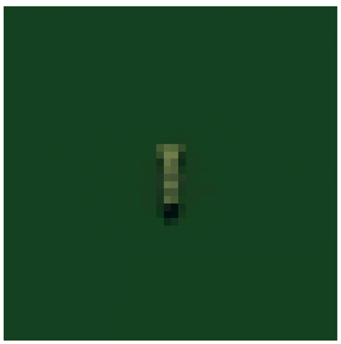 |  | 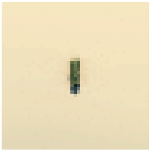 |
| Background condition | Concrete | Asphalt Road | |
| simulated image | 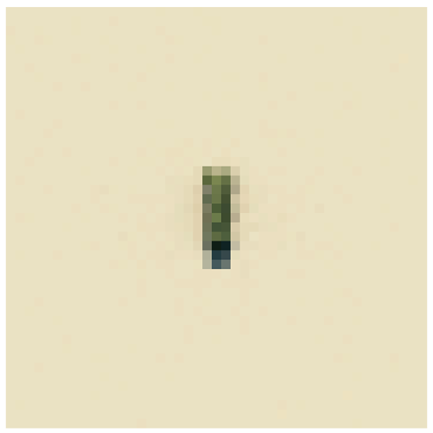 | 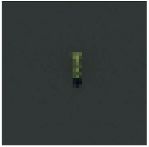 |
| solar azimuth angle | 180° |
| sensor altitude angle | 90° |
| sensor azimuth angle | 180° |
| background conditions | grassland |
| weather conditions | clear conditions |
| spectral resolution | 5 nm |
| spatial resolution | 1.0 m |
| Solar Altitude Angle | 15° | 30° | 45° |
|---|---|---|---|
| simulated image | 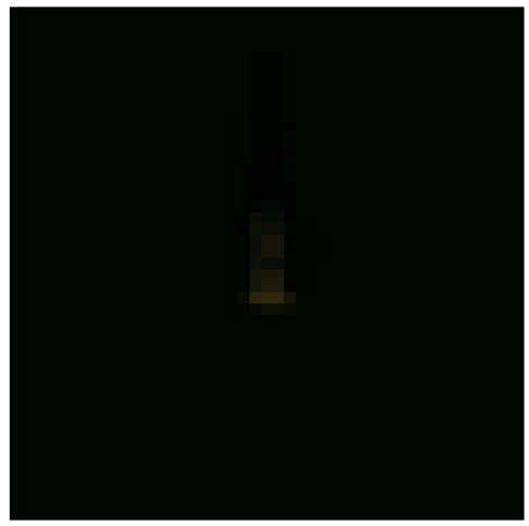 |  |  |
| Solar altitude angle | 60° | 75° | 90° |
| simulated image |  |  | 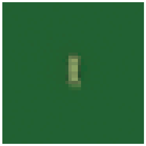 |
| solar altitude angle | 45° |
| solar azimuth angle | 180° |
| sensor azimuth angle | 180° |
| background conditions | grassland |
| weather conditions | clear conditions |
| spectral resolution | 5 nm |
| spatial resolution | 1.0 m |
| Sensor Altitude Angle | 90° | 80° | 70° |
|---|---|---|---|
| simulated image |  |  |  |
Disclaimer/Publisher’s Note: The statements, opinions and data contained in all publications are solely those of the individual author(s) and contributor(s) and not of MDPI and/or the editor(s). MDPI and/or the editor(s) disclaim responsibility for any injury to people or property resulting from any ideas, methods, instructions or products referred to in the content. |
© 2025 by the authors. Licensee MDPI, Basel, Switzerland. This article is an open access article distributed under the terms and conditions of the Creative Commons Attribution (CC BY) license (https://creativecommons.org/licenses/by/4.0/).
Share and Cite
Li, X.; Zhang, W.; Wang, B.; Qiu, H.; Jin, M.; Qi, P. OGAIS: OpenGL-Driven GPU Acceleration Methodology for 3D Hyperspectral Image Simulation. Remote Sens. 2025, 17, 1841. https://doi.org/10.3390/rs17111841
Li X, Zhang W, Wang B, Qiu H, Jin M, Qi P. OGAIS: OpenGL-Driven GPU Acceleration Methodology for 3D Hyperspectral Image Simulation. Remote Sensing. 2025; 17(11):1841. https://doi.org/10.3390/rs17111841
Chicago/Turabian StyleLi, Xiangyu, Wenjuan Zhang, Bowen Wang, Huaili Qiu, Mengnan Jin, and Peng Qi. 2025. "OGAIS: OpenGL-Driven GPU Acceleration Methodology for 3D Hyperspectral Image Simulation" Remote Sensing 17, no. 11: 1841. https://doi.org/10.3390/rs17111841
APA StyleLi, X., Zhang, W., Wang, B., Qiu, H., Jin, M., & Qi, P. (2025). OGAIS: OpenGL-Driven GPU Acceleration Methodology for 3D Hyperspectral Image Simulation. Remote Sensing, 17(11), 1841. https://doi.org/10.3390/rs17111841