Abstract
To study the influence of speed brake deflection on remote sensing grayscale images and the radar cross section (RCS) of aircraft, we present a comprehensive method based on remote sensing modeling and dynamic electromagnetic scattering. The results indicate that grayscale images from ground remote sensing can capture the hierarchical information of various reference objects and water bodies. When the target aircraft enters the observation area, complex ground reference objects may blur the grayscale features of the speed brake. The RCS of the speed brake shows strong dynamic characteristics under the example of the forward azimuth, where the maximum variation can reach 43.433 dBm2. When the speed brakes on both sides dynamically deflect, the aircraft’s RCS in the lateral azimuth will fluctuate significantly in the first half of the observation time, and those in the forward and backward azimuths will show clear dynamic characteristics in the second half of the observation time. Low grayscale ground reference and water body boundaries/areas are beneficial for distinguishing the deflection of the deceleration plate. The comprehensive method proposed here is effective for studying remote sensing grayscale images and the dynamic RCS of aircraft under speed brake deflection.
1. Introduction
Remote sensing technology is widely used for observing and imaging ground vehicles, harbor ships, and low-altitude aircraft [1,2]. The speed brake is used to increase the flight resistance of an aircraft [3], and it disrupts the original surface of the fuselage after opening beyond a certain angle. Thin-plate speed brakes not only affect the radar cross section (RCS) of aircraft but also pose challenges for remote sensing imaging of low-altitude aircraft projected against the ground.
By analyzing the motion characteristics of the target object, such as its speed and direction, remote sensing technology can be used to identify and track moving targets. For some large aircraft and flying wings, a spoiler can be installed on the upper surface of the wing to assist in deceleration [4], while the speed brakes of some fighters are positioned at the sides or the back of the fuselage. Airborne hyperspectral data are used to provide ground reference data for spatial expansion [5]. High-precision grid generation technology was used to process the surface of a flat plate in [6]. Under different flap deflections, a numerical study was carried out on a two-dimensional airfoil with an upper deflection spoiler in [7,8]. In [9,10,11], the differences between the two kinds of drag control surfaces are compared, and the mechanism of their effects on the aerodynamics and stability of flying wing aircraft is revealed. In order to alleviate the challenges posed by high-order differential templates, a special grid configuration is introduced in [10], where there is an overlap zone between coarse and fine grids. The dynamic electromagnetic scattering characteristics of the blades were determined and are discussed in [12]. Based on the optimal control allocation algorithm of envelope coordinate transformation, the control characteristics of a split-resistance rudder are analyzed in [13,14,15]. Quadcopter aircraft can fly in complex and hazardous environments and make remote sensing images to detect crop nutrition and weed infestation [16]. The numerical simulation of a typical two-dimensional multi-element wing with a spoiler deflecting downward was carried out in [17] by using computational fluid dynamics. An immune operator is used to optimize the undetermined coefficients of a parameter model of carrier-based aircraft in [18]. Opening the speed brake makes an aircraft slow down in a short time, which is beneficial for small-radius maneuvering turns and aerial refueling [19]. Solving the dynamic electromagnetic scattering of speed brakes on both sides of a tail has become a legacy problem.
Microwaves have the ability to penetrate clouds and vegetation, which enables remote sensing to obtain more information than visible light bands. With the continuous improvement in detection and strike technology, the battlefield survivability of aircraft and missiles is increasingly challenging [20,21]. With the help of Monte Carlo analysis, a statistical identification system based on RCS data is presented to classify UAVs in [22]. In [18], the dynamic electromagnetic scattering features of a helicopter model with a conventional layout were investigated. A likelihood ratio test approach was employed to make decisions on the number of spectral lines based on increasing estimates in [23]. For tailless aircraft, flaps, speed brakes, and a built-in weapon cabin are important parts of the overall design [24]. The dynamic electromagnetic scattering characteristics of rotors with varying pitch were studied in [25], and the physical theory of diffraction (PTD) was used to determine the edge contribution. Based on the quasi-static principle (QSP), the RCS of the rotor is calculated using physical optics (PO) and the equivalent current method in [26]. Combined with the forward–backward algorithm, the iterative physical optics (IPO) method was used to calculate the RCS of an open cavity in [27,28,29]. Machine learning and remote sensing techniques were used to analyze the water quality of Lake Ranko in southern Chile in [30]. In [31,32], a triangular facet was used to discretize the surface, and IPO was used to calculate the electromagnetic scattering characteristics of the target. The RCS of a Y-shaped quadrotor was calculated and analyzed in [33]. In [34], the multiple scattering model is introduced and the diffraction imaging was used to detect the internal three-dimensional structure of the sample. On the basis of the convolutional neural network and RCS sequence encoding, a spatial micro-motion approach is established for target classification [35]. The microwave darkroom testing of full-size machines and the rental of high-altitude remote sensing aircraft for observation require huge economic costs and human resources, so the remote sensing modeling of aircraft with speed reducers has become a legacy issue.
As mentioned, conducting multiple remote sensing and RCS tests on real aircraft will consume significant human resources and economic costs. The mechanism of the effect of speed brakes on aircraft stealth characteristics needs to be explored, while the remote sensing imaging of thin-plate speed brake plates against complex ground backgrounds needs to be performed. This study attempts to establish a comprehensive analysis method for remote sensing at low altitude and for the RCS characteristics for an aircraft with a deflected speed brake. The dynamic RCS calculation is of academic significance for the stealthy design and analysis of speed brakes. The remote sensing imaging method has engineering value for the grayscale analysis of details such as aircraft control surfaces.
This paper is organized as follows: the method is described in Section 2, and the model of the aircraft with a speed brake is provided in Section 3; the relevant remote sensing imaging and electromagnetic scattering characteristics are analyzed and discussed in Section 4; and, finally, the conclusion of the entire text is presented in Section 5.
2. Method Description
A schematic of the comprehensive method for remote sensing and the RCS is presented in Figure 1, where the remote sensing aircraft can appear at designated positions at high altitude and emit microwaves in simulated flight tests. xsyszs represents a coordinate system fixed on the remote sensing aircraft. The target aircraft is set to simulate flight in low-altitude space. Radar vehicles can move flexibly on the ground to reach designated directions, where xgygzg refers to a coordinate system fixed on the ground.
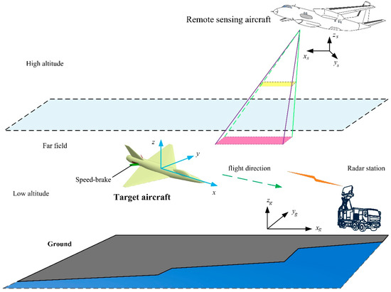
Figure 1.
A diagram of remote sensing and electromagnetic scattering for the aircraft.
2.1. Remote Sensing Modeling
When the narrow pulse emitted by the sensor from the remote sensing aircraft at a certain moment is returned by the target surface, the distance from the sensor to the target object can be calculated based on the time difference in this process:
where R refers to the distance between the target and the sensor and c is the propagation speed of the electromagnetic waves. t1 refers to the time of transmission, and t2 stands for the time of reception.
A schematic diagram of the projection difference in the sensor image is displayed in Figure 2, where H stands for the height of the sensor and ∆h is the height of point P. The projection difference can be expressed in the following form:
where refers to the projection difference and RP represents the distance from the sensor to point P. Note the following relationship:
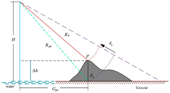
Figure 2.
A schematic diagram of the projection difference for a ground target point.
Then, the following expression can be obtained:
The projection difference can be calculated as follows:
Considering that << RP,
In order to make remote sensing images easier to recognize, image transformation and enhancement techniques are commonly used. For the movement and transformation of the image center,
where Xc0 and Yc0 represent the original center coordinates of the image, respectively. Xct and Yct represent the center coordinates of the transformed image, respectively. For the changes in image grayscale,
where Vg0 is the original image grayscale and Vgt stands for the grayscale value of the image after linear transformation. Synthetic aperture radar (SAR) requires storing radar echoes, and since the data are not collected simultaneously, it is necessary to perform calculations on the signals received within a certain time interval. Unlike SAR technology, the grayscale distribution here comes from the electromagnetic scattering characteristics of transient targets within a specific observation area. There are many reference objects of different shapes and large areas of water distributed on the ground. With the help of computer technology, the target aircraft can perform multiple independent flights in the observation area; thus, the projection of the target on the ground can appear as many key positions on the ground as possible.
2.2. Dynamic Electromagnetic Scattering
The electromagnetic scattering analysis method presented here mainly includes two modules, multiple tracking, and dynamic scattering. The former is based on iterative technology and is mainly used to reflect the characteristics of the complex scattering area of the target surface. The latter aims to fully explore the dynamic impact of speed brake deflection on the aircraft.
When a single speed brake is opened, it forms a dihedral angle with the nearby fuselage surface, which may cause multiple reflections of the incident wave. The scattering field of the target surface can be expressed as
where r is the central coordinate of a triangular surface element on the surface of the scatterer. J represents the surface current. r′ represents the central coordinate of another triangular surface element. S is the integral surface and ds′ is the integral element. k is the wave number in free space. G is the Green function of free space.
For the action of opening the speed brakes on both sides of the fuselage, the multiple scattering of the incident wave in the acute corner area by dihedral angles is clearer under some azimuth angles. The introduction of the iterative technique enables the contribution of multiple scattering to be captured. Then, the facet current can be obtained as
where is the outward normal unit vector of the facet. The subscript of the current is used to record the number of iterations.
For the irradiation area of the target,
where SI is the illumination area, SD is the dark area, and Hi is the incident magnetic field.
Thus, the surface current can be updated to
Consider the change in the difference in surface current:
where Rc is the convergence rate of the current. Then, the electric and magnetic fields on the target surface, respectively, can be updated to
where ω is the electromagnetic wave’s angular frequency, M(r′) is the magnetic current of the facet at r′, μ is the permeability coefficient, and ε is the dielectric permittivity. Considering that the speed brake and the fuselage have more edge features, PTD is used to calculate the edge diffraction contribution; thus, the RCS of the target can be expressed as follows:
where σ is the RCS, subscript F refers to the facet contribution, and E represents the edge contribution. NE is the number of edges and NF is the number of facets.
The electromagnetic scattering diagram of the aircraft speed brakes is shown in Figure 3, where Frh represents the radar wave frequency and horizontal polarization. α is the azimuth between the radar station and the aircraft, and β is the elevation angle. For the same incident wave, the speed brake will show different deflection abilities to electromagnetic waves at different opening angles.
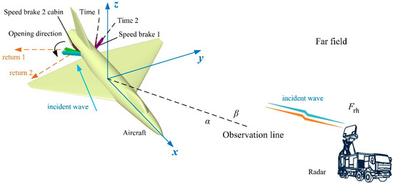
Figure 3.
Schematic of dynamic electromagnetic scattering of speed brake.
When speed brake 1 starts to open,
where Mb1 is the grid coordinate matrix of speed brake 1 and the superscript indicates a specific change operation. mb1 is the model of speed brake 1. Ab is the opening angle of the speed brake and additional numerical subscripts are used to distinguish different speed brakes. Xb1 is the distance from the deflection axis of speed brake 1 to the yz plane, and Yb1 is the distance from the deflection axis of speed brake 1 to the xz plane.
Then, consider the deflection of speed brake 2 as follows:
where Mb2 and mb2 are the grid coordinate matrix and model of speed brake 2, respectively. Xb2 and Yb2 are the distances from the deflection axis of speed brake 2 to the yz and xz planes, respectively.
For the model of the whole aircraft,
where t is time, ma is the aircraft model, and mf is the model of the fuselage. We can return the obtained speed brake model to the initial position and then combine it with the fuselage as follows:
where Ma and Mf refer to the grid coordinate matrices of the aircraft and fuselage, respectively. If the fuselage attitude remains unchanged in the current coordinate system,
For a given incident wave, the target surface is illuminated:
To analyze the scattering characteristics of the target surface,
where Isc refers to the customized scattering intensity; Kcd is the control factor of color depth; σf refers to the facet RCS under the current condition; σfm and σfn represent the maximum and minimum of the facet RCS, respectively; and Bcm and Bcn are the upper and lower boundaries of the current color window, respectively.
The dynamic RCS of the target can be calculated as follows:
where Tob is the observation duration and Tdd is the deflection duration of the speed brake.
The validation of the presented method is shown in Figure 4, where ωb is the angular velocity at which the speed brake opens outwards, and the additional numeral subscript is used to distinguish the speed brake number. The reference curve is the result of PO+MOM (method of moment)/MLFMM (multilayer fast multipole method) combined with QSP [25], where MOM is a numerical analysis technique that uses integral equations to solve electromagnetic scattering problems. For the RCS at t = 3.18 s, it can be seen that the red dotted and green solid lines are generally similar, where the mean RCSs are 12.4664 and 12.7982 dBm2, respectively. The maximum of the reference data is 33.74 dBm2 at an azimuth of 92°, and that of another curve is 33.46 dBm2 at an azimuth of 92.25°. For the RCS at α = 27°, speed brake 2 remains closed, and speed brake 1 conducts dynamic deflection in this case, where the trend and fluctuation amplitude of the two RCS curves are basically consistent. These results show that the presented method is feasible and accurate for studying the dynamic impact of the speed brake on the aircraft’s RCS.
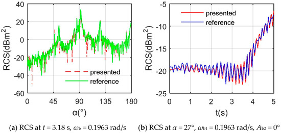
Figure 4.
Method validation on RCS of aircraft, Frh = 7 GHz, β = 0°.
3. Model Establishment
The speed brake has a certain thickness, which results in a shallow cabin space at the installation position on the fuselage surface, as in Figure 5, where Awl is the sweep angle of the leading edge of the wing and Awt is the forward sweep angle of the trailing edge of the wing. Lrf is the distance from the rear vertex of the speed brake chamber to the rear end face of the fuselage. Atl is the tilt angle of the leading edge of the vertical tail. Lf and Wf represent the length and width of the fuselage model, respectively. Hv is the distance from the top of the vertical tail to the xy plane. When the speed brake is not opened, its outer surface forms a closed hole with the nearby fuselage wall.
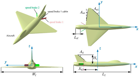
Figure 5.
Aircraft model with speed brakes open.
This aircraft adopts the aerodynamic configuration of a lower single wing and a vertical tail, and its main dimensions are shown in Table 1. The wing and the vertical tail adopt a clear swept back design, and the two speed brakes are symmetrically distributed on both sides of the rear fuselage engine compartment.

Table 1.
Main dimensions of aircraft model.
The details of the model of speed brake 1 are shown in Figure 6, where the two speed brakes adopt the same shape layout and take into account the preliminary low-scattering characteristic configuration. Lb1, Wb1, and Hb1 are the length, width, and height of the speed brake, respectively. Ltv is the convex distance of the tail vertex of the speed brake. Lbe and Hbe are used to limit the beveling of the edge of the speed brake. The main dimensions of speed brake 1 are shown in Table 2.
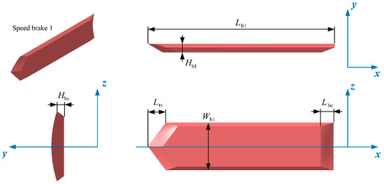
Figure 6.
Model of speed brake 1.
Table 2.
Main dimensions of speed brake 1.
The surface of the object model is discretized by using triangular patches, where high-precision unstructured grid technology is used to process the surface of the speed brake and fuselage model, as shown in Figure 7. For the small areas such as the edge of the speed brake, the leading edge of the wing, and the edge of the vertical tail, the method of increasing the grid density is adopted. The global minimum partition size is used to further improve the quality of mesh generation, as shown in Table 3. The independence verification of the adopted grid technology is shown in Figure A1 of Appendix A.
Figure 7.
Mesh treatment of fuselage and speed brake.
Table 3.
Grid size on various regions of aircraft.
4. Results and Discussion
4.1. Analysis of Remote Sensing
The grayscale remote sensing image taken before the target aircraft has entered the observation zone is presented in Figure 8, where the grayscale features in the upper left and lower right of the image have undergone significant layering. Around x = −36.27 m and y = 20.22 m, a gray area (grayscale about −150) resembling a sickle shape appears. Observing from this gray area towards the negative y-axis, a light gray reference object (grayscale from −130 to −35) in the shape of a bent line segment can be observed. At the line of y = −8.816 m, some trapezoidal gray reference objects (grayscale about −138) appear regularly. Because the natural frequency of water molecule vibration happens to be within the frequency range of microwaves, it is easy for microwaves to transfer their energy to water molecules when irradiating water bodies. The grayscale of this area can be considered as an instantaneous calculation of a specific region by this remote sensing modeling method, while the SAR data are not collected simultaneously. These results indicate that it is feasible to use the established remote sensing imaging method to capture the grayscale features of ground reference objects.

Figure 8.
The grayscale image taken before the target aircraft has entered the remote sensing observation area, β = 27°, Frh = 6 GHz, α = 29°.
The grayscale image when the target has entered the observation region is shown in Figure 9, where the grayscale distribution in the upper left area of the image has undergone significant changes, noting that the coordinates of the center of the image have been transformed to those of the center of the target aircraft. Aluminum alloy, stainless steel, and carbon fiber are common skin materials, and in this modeling analysis, the aircraft skin is considered to be an ideal conductor. Around x = −5.226 m and y = 28.4 m, the originally sickle-shaped backtracking area has turned light gray (grayscale about −52) due to a significant increase in the elevation angle of the incident wave. At x = −1.079 m and y = 1.553 m, the leading and trailing edges of a triangular wing can be identified, where the grayscale of the nose and tail can also be observed when viewed along the x-axis. At the current observation scale (without local magnification measures), it is difficult to capture the grayscale features of the speed brake plates because they have a low thickness and are designed with low-scattering features at the edges, where the actual preset opening angle of the speed brake is 17.2125° in this flight test. These results indicate that it is feasible to use the established remote sensing method to capture a target aircraft entering the observation area, while additional local magnification measures are needed to further observe the deceleration plate.
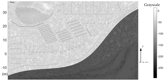
Figure 9.
The grayscale remote sensing image taken when the target has entered the remote sensing observation region, β = 65°, Frh = 7 GHz, α = 51°.
The grayscale image taken when the target aircraft has entered the observation area is presented in Figure 10, where the coordinates of the center of the remote sensing image have been converted to those of the center of the target aircraft. At x = −1.547 m and y = 2.23 m, it can be observed that the triangular wing obstructs a portion of the horizontal segment of the reference object in the shape of the bent line segment on the ground. The grayscale of the front fuselage (grayscale about −62) and the vertical tail side (grayscale about −95) are still easily recognizable, where the top middle of the fuselage appears light gray because the curved surface cannot effectively deflect the incident wave to other directions. After a magnified observation, it can be observed that the speed brake plate on one side is in the open state, while the preset deflection angle of the speed brake is 24.3° in the flight test. Due to the absorption of incident waves by water bodies, the water in the lower right area of the image appears as an extremely low gray feature. These results indicate that the remote sensing imaging method requires multiple amplifications of local areas in the image to determine the opening angle of the speed brake plate.
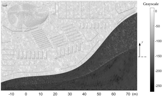
Figure 10.
The grayscale image taken when the target aircraft has entered the remote sensing observation zone, β = 72°, Frh = 8 GHz, α = 120°.
The remote sensing image taken when the target has entered the observation region is shown in Figure 11, where the position and heading of this aircraft target can be easily determined under current observation conditions. Due to changes in azimuth and radar wave frequency, the grayscale distribution in the lower right area of the image has undergone some alterations. At x = −4.102 m and y = −0.9139 m, the opening state and deflection angle of the speed brake can be observed without local amplification, and the deflection angle is 30.71°. Around y = 23.86 m, a large number of tilted gray narrow reference objects (grayscale about −73) can be identified. Because the grayscale contrast between the surface of the target aircraft and the nearby water bodies is very distinct, the outline of the aircraft and the side features of the speed brake plates are displayed. These results indicate that it is feasible to use this remote sensing method to capture the grayscale details of the opened speed brake plate under current observation conditions.
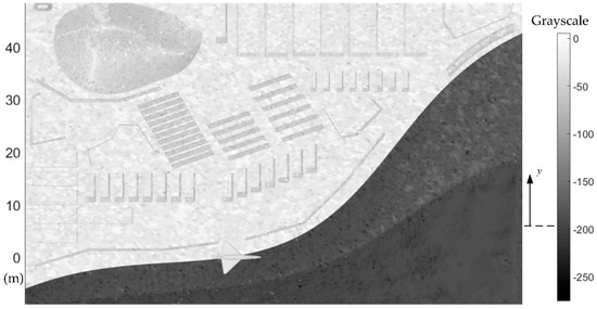
Figure 11.
The grayscale remote sensing image taken when the target has entered the remote sensing observation area, β = 81°, Frh = 9 GHz, α = 168°.
4.2. Dynamic Scattering Analysis
Figure 12 shows that the RCS curve of a single speed brake shows more local fluctuations and a larger variation range under given observation conditions. When β = 0°, the average RCSs of the curves with α = 10 and 20° are −19.9645 and −14.2599 dBm2, respectively, where the latter shows a larger fluctuation range because the scattering contribution of the surface facet of the speed brake is enhanced. The Doppler characteristics of the reference vertex of the deceleration plate are shown in Figure A2 of Appendix A. As the azimuth angle increases to 30°, the mean RCS value of the curve further increases to −2.3951 dBm2. For the case of α = 10°, the initial value of the RCS curve decreases with the increase in the elevation angle, because the specular reflection of the speed brake irradiation area is significantly weakened. When β = 10°, the minimum value of the RCS curve is −38.083 dBm2, appearing at 0.36 s, while the average value is −24.8506 dBm2. These results indicate that the RCS level of the individual speed brakes is low due to the low-scattering profile design, while during the whole deflection process, the RCS has many fluctuations and large amplitude changes at different observation angles, which cannot be ignored.
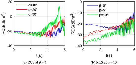
Figure 12.
Dynamic RCS of speed brake 1, Frh = 7 GHz, ωb1 = 0.1963 rad/s.
Figure 13 shows that the scattering characteristics of the outer surface of the single speed brake increase with the increase in the opening angle. For the case of t = 0.45 s, the narrow surface on the upper side of the speed brake is light cyan (about −110 dBm2) under the irradiation of the current incident wave, while light yellow and orange (about −68 dBm2) are distributed on the outer surface of the speed brake. When t = 1.5 s, the scattering intensity of the outer surface of the speed brake has been enhanced where the opening angle is 16.875°. As the time increases to 5.7 s, the scattering intensity of the outer surface of the speed brake is significantly enhanced, and some facets are dark orange (about −48 dBm2). Since the narrow surfaces around the speed brake are sharpened to deflect the incident wave towards the non-threatening direction, the outer surface of the speed brake acts as the main scattering source.
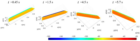
Figure 13.
Surface scattering characteristics of speed brake 1, Frh = 7 GHz, ωb1 = 0.1963 rad/s, RCS unit: dBm2, α = 12.25°, β = 0°.
Figure 14 indicates that the mean level of the RCS curve is significantly reduced with the increase in elevation angle. When β = 0°, the RCS curve reaches a maximum of 20.3689 dBm2 at an azimuth of 263.5°, because the inner surface of the speed brake is mainly a plane design, and it is almost perpendicular to the incident wave where the opening angle of the speed brake is 6.75°. As the elevation angle increases from 0 to 2°, the mean RCS decreases from −20.3689 to −2.2610 dBm2, because the strong scattering sources on the outside and inside of the speed brake are slightly weakened. When β = 5°, the RCS value of this curve at most azimuths is significantly lower than those of the other two curves, while the mean RCS further decreases to −5.6170 dBm2. In this case, the maximum peak value is 17.0677 dBm2, appearing at an azimuth of 83.25°. In addition, the three RCS curves are not symmetrical, because the outside and inside surfaces of the speed brake adopt different designs. The outside surface here is integrated with the nearby fuselage surface, while the inside surface is composed of a plane and several narrow surfaces. These results show that under the current observation conditions, the increase in elevation angle is conducive to reducing the mean and peak levels of the speed brake’s RCS.
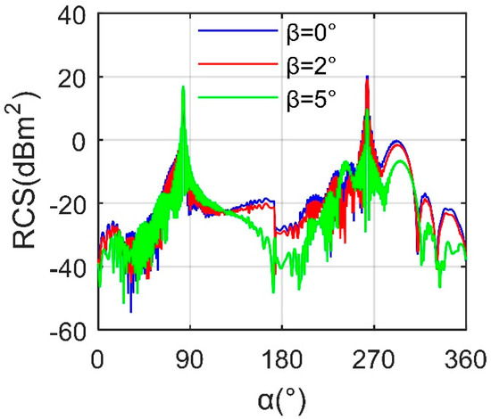
Figure 14.
RCS of speed brake 1, Frh = 7 GHz, ωb1 = 0.1963 rad/s, t = 0.6 s.
Figure 15 shows that the opening of a single speed brake can bring many clear dynamic changes to the forward RCS of the aircraft. For the case of α = 12°, the maximum value of the RCS curve is −5.9864 dBm2 and the average is −13.4417 dBm2, where the whole curve fluctuates less in the first half and more intensely in the second half. When α = 18°, the initial value of the RCS curve decreases significantly, while the mean value is −13.7206 dBm2. With the azimuth angle increasing to 25°, the mean value and fluctuation range of the RCS curve are greatly improved. It can be seen that the green solid line is above the other two curves at most azimuth angles, where the average RCS of α = 25° curve reaches −2.1778 dBm2 and the maximum value is 13.97 dBm2. The main reason for this improvement is the facet contribution of the outer surface of the speed brake. Because the overall scattering level of the speed brake is low, the contribution of surface scattering and edge diffraction changes alternately, resulting in continuous fluctuations in the curve. These results indicate that the deflection of a single speed brake can bring undesirable dynamic responses to the RCS of the aircraft at key forward azimuths, including mean and peak levels.
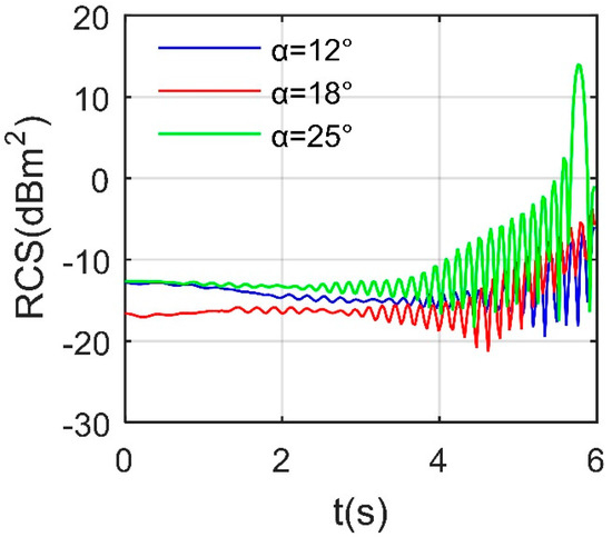
Figure 15.
Forward RCS of aircraft, Frh = 7 GHz, ωb1 = 0.1963 rad/s, β = 0°, Ab2 = 0°.
Figure 16 reveals that during the first third of the observation time, the deflection of the speed brake will bring significant fluctuations to the RCS of the aircraft at the lateral azimuth angle of the example. For the case of α = 85°, this kind of fluctuation is the most intense compared with the other two curves. The mean RCS of the blue curve is 7.0309 dBm2, where the maximum and minimum peak values reach 18.4869 and 1.0313 dBm2, respectively. In the initial stage of deflection, the outer surface of the speed brake can still provide additional strong scattering sources. With the deflection angle exceeding 22.5° (after 2 s), the overall deflection ability of the outer surface of the speed brake to the radiation decreases significantly and gradually changes into a low-scattering area. The mean RCS values of α = 92 and 99° curves are 17.8876 and 0.1728 dBm2, respectively. Although the mean values of the three RCS curves differ greatly, the dynamic effects caused by the deflection of the speed brake cannot be covered by the fuselage RCS.
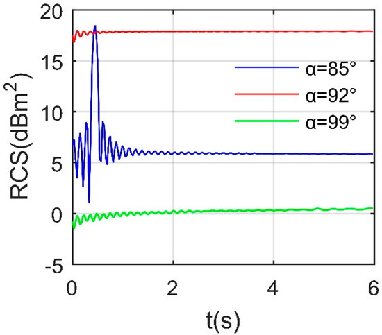
Figure 16.
Side RCS of aircraft, Frh = 7 GHz, ωb1 = 0.1963 rad/s, β = 3°, Ab2 = 0°.
Figure 17 shows that a large opening angle of the speed brake will significantly change the local peak position of the aircraft RCS. When Ab = 9.1125°, the mean RCS of the curve is 4.9342 dBm2 and the maximum reaches 22.5325 dBm2 appearing at an azimuth of 85°. In this case, the outward opening angle of the two speed brakes is small, and the ability to deflect the incident wave is close to that of the nearby fuselage surface. For the case of Ab = 12.4875°, the maximum peak is 22.7803 dBm2 and the occurrence position remains unchanged. It can be seen that there are many peaks in these curves near the lateral 90 and 270° azimuths due to the scattering contribution of the fuselage side and the vertical tail. In addition, for the three curves with Ab greater than 29°, new local peaks appear near the 47.25° azimuth; meanwhile, with the increase in the speed brake opening angle, the azimuth of this new peak appears to decrease. This peak shift also occurs around the azimuths of 132.3, 227.8, and 312.8°, while the position where the maximum peak occurs is still maintained at an azimuth of 85°. The mean RCSs of the Ab = 29.7 and 54° curves are 4.8715 and 4.9483 dBm2, respectively. In the fixed angle opening mode, the impact of the speed brake on the aircraft RCS is mainly reflected in the appearance of a local peak value, followed by the mean RCS.
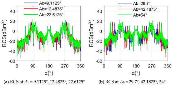
Figure 17.
RCS of aircraft, Frh = 7 GHz, β = −5°.
Figure 18 shows that at the current elevation angle, there is a small difference in the maximum and average values of RCS curves at different speed brake opening angles. For the case of Ab = 11.8125°, the RCS curve is generally M-shaped and has more local peaks in the lateral direction, where the mean is 5.7564 dBm2 and the maximum reaches 26.1666 dBm2 appearing at an azimuth of 85.5°. As the opening angle of the speed brake increases to 32.4°, the average of the RCS curve decreases to 5.7142 dBm2, while the maximum increases to 26.29 dBm2, occurring at an azimuth of 85.5°. It is worth noting that this RCS curve has a peak value of more than 16.75 dBm2 at the azimuth angles of 57.5 and 302.5°. When Ab = 43.2°, the mean value of the RCS curve is further reduced to 5.6755 dBm2, where the maximum is 26.2624 dBm2 at an azimuth of 85.5°. A peak value of 16.55 dBm2 appears at an azimuth of 46.5° because the incident wave is almost perpendicular to some panels on the outer surface of speed brake 1, which greatly enhances the scattering intensity of these panels. This phenomenon is also reflected in speed brake 2 with an azimuth angle of 313.5°. Under the current observation conditions, the impact of the speed brake on the aircraft RCS is mainly reflected in the local peak and curve shape, followed by the mean and maximum.
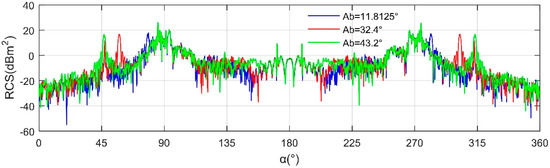
Figure 18.
RCS of aircraft, Frh = 7 GHz, β = 7°.
4.3. Comprehensive Discussion
Figure 19 shows that with the opening of the speed brake, the inner wall of the speed brake chamber may provide some strong scattering sources. For the case of α = 15° where t = 1.83 s, both speed brakes are opened outwards by 20.5875°. The outer surface of speed brake 1 is light orange (about −62 dBm2) because, in this case, the electromagnetic wave is incident from above, and the outer surface of speed brake 1 provides some scattering contributions. The narrow wall at the rear of the cabin of speed brake 1 is under the irradiation of the incident wave, and the current design of its shape cannot deflect an incident wave in a non-threatening direction; thus, it presents a small amount of red (about −40 dBm2). Due to the chamfered narrow surface design, the upper edge of speed brake 2 is a light green color (about −90 dBm2). For the whole aircraft, the vertical tail, the side of the rear fuselage, the curved surface near the leading edge of the wing, the front of the cockpit, and the nose show strong scattering characteristics. Considering the case of α = 27° where t = 3.36 s, the opening angle of the speed brake reaches 37.8°. The surface of speed brake 1 changes to a deeper orange (about −58 dBm2), while its cabin wall also appears more orange–red (about −45 dBm2) and red (about −40 dBm2). The increase in azimuth further strengthens the original strong scattering area of the aircraft; the original orange–red on the surface of the vertical tail changes to bright red; most areas on the side of the cockpit are red; and the red area on the side of the fuselage is deepened and extended to the back of the fuselage. Under the current observation conditions, although the fuselage side and vertical tail areas account for strong scattering contributions, the variation in the scattering intensity of the speed brake can still be reflected.
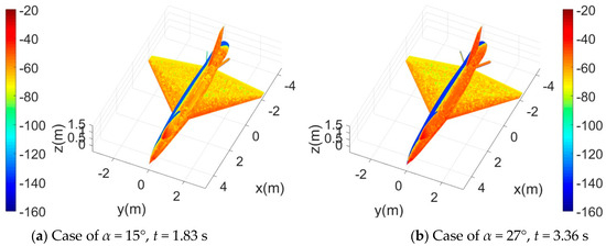
Figure 19.
Surface scattering characteristics of aircraft, Frh = 7 GHz, RCS unit: dBm2, ωb = 0.1963 rad/s, β = 6°.
Figure 20 indicates that the continuous deflection of the two speed brakes brings dynamic changes to the RCS at the forward azimuth angle of the aircraft. When α = 3°, the RCS curve reaches a maximum of −14.4622 dBm2 at t = 5.85 s, while the initial value is −25.91 dBm2. The whole curve shows more fluctuation, and the fluctuation amplitude is greater in the second half of the observation time. The mean RCSs of the α = 3, 6, and 9° curves are −23.13, −23.9752, and −1.7561 dBm2, respectively. Due to the increase in azimuth, the dynamic response of speed brake 2 has just been significantly weakened when α = 9°. In addition to the significant increase in the average RCS of the aircraft, the fluctuation amplitude of the curve of α = 9° is smaller than those of the other two curves within the current observation range. During the first half of the observation time, the RCS curve with α = 3 and 6° can still show some dynamic changes, while the RCS curve with α = 9° has little fluctuation within the current observation range. These results show that when the speed brakes are deflecting, the RCS difference of the aircraft under different forward azimuth angles is mainly reflected in the mean value and fluctuation amplitude.
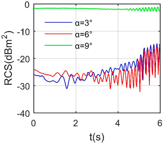
Figure 20.
Forward RCS of aircraft, Frh = 7 GHz, ωb = 0.1963 rad/s, β = 8°.
Figure 21 shows that the speed brake mainly affects the side RCS of the aircraft in the first half of the observation time and mainly affects the tail RCS of the aircraft in the second half of the observation time. The two RCS curves with α = 81 and 83° are similar in terms of mean, peak, and shape, where the mean RCS of the α = 81° curve is 9.6552 dBm2 and the maximum is 19.1092 dBm2 at t = 0.81 s. As the azimuth increases to 87°, the mean value of the RCS curve rapidly increases to 17.8579 dBm2, while the change range of the whole curve reaches 16.66 dBm2 because the scattering contribution is provided by some areas and narrow surfaces under the outer surface of speed brake 1, and there is a diffraction contribution at the lower edge of speed brake 2. For the tail cases, the shape of the RCS curve with α = 185° is completely different from the other two curves. The average RCSs of the α = 182 and 185° curves equal 2.2539 and −14.3263 dBm2, respectively. During the first half of the observation period, the curve of α = 185° fluctuates a little near −20.21 dBm2. When t = 4.71 s, this curve reaches its lowest value at –28.1136 dBm2, while the maximum value of −6.143 dBm2 occurs at t = 5.46 s. For α = 189°, since the narrow tail surface and edge of the speed brake provide a small amount of scattering contribution during the first half of the observation time, the fluctuation in this tail RCS curve in this case can hardly be reflected in the current observation range. Under the given observation conditions, the dynamic characteristics of the side and tail RCS of the aircraft are clear, and the differences are reflected in the main concentration period of the fluctuation, curve peak, and mean.
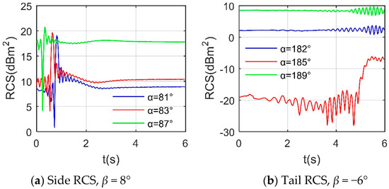
Figure 21.
Dynamic RCS of aircraft, Frh = 7 GHz, ωb = 0.1963 rad/s.
The grayscale remote sensing image when the target aircraft has entered the remote sensing observation zone is presented in Figure 22, where the projection of the target aircraft in the grayscale distribution of the water body area is clearly displayed. At x = −3.508 m and y = 0.9082 m, the open state of the speed brake can be determined, and the deflection angle can be calculated as 43.2°. Observing along the curved boundary of the water body region, several gray bands in the shape of bent line segments can be found. Around the line of y = 37.68 m, several square-shaped light-gray ground reference objects (grayscale about −25) can be identified. Due to the significant difference in gray levels between the surface of the aircraft and the water area, the deflection details of the speed brake plate can be observed without local magnification. By zooming in multiple times, the deflection angle of the speed brake plate can be calculated and obtained. Overall, the dynamic deflection of the thin speed brake can cause sharp changes in the critical azimuth RCS of the aircraft, while also challenging the detailed observation of remote sensing imaging.
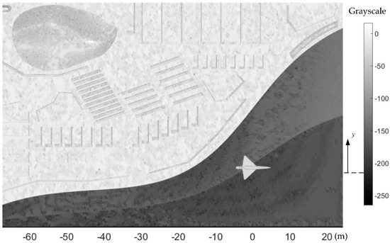
Figure 22.
The grayscale remote sensing image taken when the target aircraft has entered the remote sensing observation region, β = 83°, Frh = 7 GHz, α = 279°.
5. Conclusions
Based on the established comprehensive measurement method, remote sensing imaging of aircraft entering the observation area is obtained, and the dynamic RCS impact caused by the speed brake is analyzed. According to these investigations and discussions, the following conclusions can be drawn:
- (1)
- This remote sensing imaging method can capture the grayscale characteristics of many reference objects on the ground. When the target aircraft enters the observation area, some complex ground reference objects can easily confuse the grayscale projection of the thin speed brake with the ground without taking local magnification measures.
- (2)
- The dynamic RCS of the speed brake at the forward azimuth shows a large amplitude in the second half of the deflection process, where the increase in elevation angle can reduce the mean and initial value of this dynamic RCS. When the speed brake is deflected on one side, the amplitude of the change in RCS at an example forward azimuth of the aircraft may exceed 33.36 dBm2, while the dynamic characteristics and mean value of the aircraft’s RCS vary greatly under different lateral azimuths.
- (3)
- When two speed brakes are opened at a fixed angle, this will introduce a local peak value to the RCS–azimuth curve of the aircraft. The first half of the dynamic deflection of the two speed brakes will introduce large fluctuations to the RCS of the aircraft in the lateral azimuth. When the projection of the target aircraft crosses the water boundary or enters the water area, the fuselage, wings, and vertical tail are easily recognizable, and the opening state and deflection angle of the speed brake can be determined.
Funding
This work was supported by the Project funded by China Postdoctoral Science Foundation (Grant Nos. BX20200035, 2020M680005).
Data Availability Statement
The original contributions presented in the study are included in the article, and further inquiries can be directed to the corresponding author.
Conflicts of Interest
The author declares no conflicts of interest.
Appendix A
The grid independence verification of speed brake 1 is presented in Figure A1, where Ntf is the number of triangular elements on the surface of the brake plate. The increase in the density of edge grid nodes and surface nodes will lead to an increase in the number of grids on the model surface, and it can be observed that the RCS results eventually tend to stabilize (14.12 dBm2); when Ntf = 4.589 × 10⁴, the RCS indicator is 14.092 dBm2. These results indicate that the grid technique used to treat the model surface is feasible and reliable.
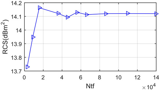
Figure A1.
Grid independence verification of speed brake 1, α = 30°, β = 0°, Frh = 7 GHz, ωb1 = 0.1963 rad/s, t = 5.34 s.
The Doppler feature of the speed brake 1 is shown in Figure A2, where Fdt is the Doppler frequency of the outer vertex of the brake plate [36], Fdtb is the Doppler frequency of the outer vertex of the lower edge of the deceleration plate, ωb1 = 0.1963 rad/s. The dynamic deflection of the deceleration plate will bring Doppler effect to actual observations. When the target is a flexible body, the contributions of motion effects and geometric shape changes require additional calculations as provided in the supplementary information in reference [37].
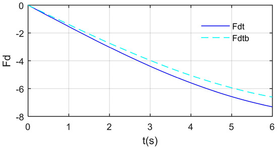
Figure A2.
Doppler feature of the speed brake 1, Frh = 7 GHz, α = 0°, β = 0°.
References
- Lockhart, K.; Sandino, J.; Amarasingam, N.; Hann, R.; Bollard, B.; Gonzalez, F. Unmanned Aerial Vehicles for Real-Time Vegetation Monitoring in Antarctica: A Review. Remote Sens. 2025, 17, 304. [Google Scholar] [CrossRef]
- Liang, H.S. Stealth technology for radar onboard next generation fighter. Mod. Radar. 2018, 40, 11–14. [Google Scholar]
- Cui, W.; Liu, J.; Sun, Y.; Li, Q.; Xiao, Z. Airbrake controls of pitching moment and pressure fluctuation for an oblique tail fighter model. Aerosp. Sci. Technol. 2018, 81, 294–305. [Google Scholar] [CrossRef]
- Wang, G.; Zhang, M.H.; Mao, J.; Sang, W.M.; Chen, Z.L.; Wang, L. and Zhang, B. High-lift technology for spoiler on blended-wing-body civil aircraft. Acta Aeronaut. Et Astronaut. Sinica 2019, 40, 623045. [Google Scholar]
- Teillet, P.M.; Fedosejevs, G.; Gauthier, R.P. Operational radiometric calibration of broadscale satellite sensors using hyperspectral airborne remote sensing of prairie rangeland: First trials. Metrologia 1998, 35, 639. [Google Scholar] [CrossRef]
- Cheng, X.Q.; Wong, C.W.; Hussain, F. Flat plate drag reduction using plasma-generated streamwise vortices. J. Fluid Mech. 2021, 918, A24. [Google Scholar] [CrossRef]
- Wang, W.; Liu, P. Numerical Study of Spoiler Aided by Flap on Roll Control and Airbrake Civil. Aircr. Des. Res. 2017, 1, 38–44. [Google Scholar]
- Yan, X.; Chen, R. Augmented flight dynamics model for pilot workload evaluation in tilt-rotor aircraft optimal landing procedure after one engine failure. Chin. J. Aeronaut. 2019, 32, 92–103. [Google Scholar] [CrossRef]
- Zuo, L.X.; Wang, J.J. Experimental study of the effect of AMT on aerodynamic performance of tailless flying wing aircraft. Acta Aerodyn. Sin. 2010, 28, 132–137. [Google Scholar]
- Mao, L.; Wang, X.; Chi, Y.; Pang, S.; Wang, X.; Huang, Q. A Three-Dimensional FDTD (2,4) Subgridding Algorithm for the Airborne Ground-Penetrating Radar Detection of Landslide Models. Remote Sens. 2025, 17, 1107. [Google Scholar] [CrossRef]
- Li, Z.J.; Ma, D.L. Control characteristics analysis of drag yawing control devices of flying wing configuration. J. Beijing Univ. Aeronaut. Astronaut. 2014, 40, 695–700. [Google Scholar]
- Zhou, Z.; Huang, J. Study of the Radar Cross-Section of Turbofan Engine with Biaxial Multirotor Based on Dynamic Scattering Method. Energies 2020, 13, 5802. [Google Scholar] [CrossRef]
- Qu, X.B.; Zhang, W.G.; Shi, J.P. Control allocation method for split-drag-rudders with asymmetrical deflection. J. Syst. Simul. 2016, 28, 627–639. [Google Scholar]
- Dash, S.M.; Triantafyllou, M.S.; Alvarado, P.V.Y. A numerical study on the enhanced drag reduction and wake regime control of a square cylinder using dual splitter plates. Comput. Fluids 2020, 199, 104421. [Google Scholar] [CrossRef]
- Liu, J.; Zheng, L.Q. Study on Flow Mechanism and Aerodynamic Characteristic of High-Lift Devices with Drooped Spoiler. J. Northwestern Polytech. Univ. 2017, 35, 813–820. [Google Scholar]
- Li, S.; Simonian, A.; Chin, B.A. Sensors for agriculture and the food industry. Electrochem. Soc. Interface 2010, 19, 41–46. [Google Scholar] [CrossRef]
- Liu, C.; Liu, P. Research on Aerodynamic Characteristics of AHDF Civil Aviation Aircraft. Aeronaut. Comput. Tech. 2021, 51, 84–87. [Google Scholar]
- Zhou, Z.; Huang, J. An optimization model of parameter matching for aircraft catapult launch. Chin. J. Aeronaut. 2020, 33, 191–204. [Google Scholar] [CrossRef]
- Li, T.S. Analysis and Treatment on Left Front Deceleration Beam Crack for a Certain Type of Aircraft. Aviat. Maint. Eng. 2019, 3, 97–99. [Google Scholar]
- Saleem, M.; Saifullah, Y. Coding Artificial Magnetic Conductor Ground and Their Application to High-Gain, Wideband Radar Cross-Section Reduction of a 2×2 Antenna Array. Phys. Status Solidi 2021, 218, 2100088. [Google Scholar] [CrossRef]
- Chen, L.; Duan, P.F.; Yuan, C. Research on development status and key technology of stealth air-to-air missiles. Aero Weapon. 2022, 29, 14–21. [Google Scholar]
- Ezuma, M.; Anjinappa, C.K.; Funderburk, M. Radar cross section based statistical recognition of UAVs at microwave frequencies. IEEE Trans. Aerosp. Electron. Syst. 2021, 58, 27–46. [Google Scholar] [CrossRef]
- Bu, L.; Fu, T.; Chen, D.; Cao, H.; Zhang, S.; Han, J. Doppler-Spread Space Target Detection Based on Overlapping Group Shrinkage and Order Statistics. Remote Sens. 2024, 16, 3413. [Google Scholar] [CrossRef]
- Yin, P.; Jia, G.W.; Yang, X.X. Research on the development of foreign military uav stealth design. Aerodyn. Missile J. 2021, 12, 69–74. [Google Scholar]
- Zhou, Z.; Huang, J. Numerical investigations on radar cross-section of helicopter rotor with varying blade pitch. Aerosp. Sci. Technol. 2022, 123, 107452. [Google Scholar] [CrossRef]
- Ye, S.B.; Xiong, J.J. Dynamic RCS Behavior of Helicopter Rotating Blades. Acta Aeronaut. Et Astronaut. Sinica 2006, 27, 816–822. [Google Scholar]
- Zhou, Z.; Huang, J. Mixed design of radar/infrared stealth for advanced fighter intake and exhaust system. Aerosp. Sci. Technol. 2021, 110, 106490. [Google Scholar] [CrossRef]
- Xu, X.; Gong, S.X. The forward-backward IPO algorithm for calculating open-ended cavities. Space Electron. Technol. 2008, 1, 72–76. [Google Scholar]
- Song, S.; Cho, C.; Oh, T. Effect of driving frequency on reduction of radar cross section due to dielectric-barrier-discharge plasma in Ku-band. IEEE Trans. Plasma Sci. 2021, 49, 1548–1556. [Google Scholar] [CrossRef]
- Rodríguez-López, L.; Bravo Alvarez, L.; Duran-Llacer, I.; Ruíz-Guirola, D.E.; Montejo-Sánchez, S.; Martínez-Retureta, R.; López-Morales, E.; Bourrel, L.; Frappart, F.; Urrutia, R. Leveraging Machine Learning and Remote Sensing for Water Quality Analysis in Lake Ranco, Southern Chile. Remote Sens. 2024, 16, 3401. [Google Scholar] [CrossRef]
- Sui, M.; Xu, X.J. Electromagnetic scattering calculation of complex structure using iterative physical optics based on curved surface patches. Chin. J. Radio Sci. 2012, 27, 892–896. [Google Scholar]
- Zhou, Z.; Huang, J. Study of RCS characteristics of tilt-rotor aircraft based on dynamic calculation approach. Chin. J. Aeronaut. 2022, 35, 426–437. [Google Scholar] [CrossRef]
- Zhou, Z.; Huang, J. Y-type quadrotor radar cross-section analysis. Aircr. Eng. Aerosp. Technol. 2023, 95, 535–545. [Google Scholar] [CrossRef]
- Zhang, T. Iterative Physical Optics and Its Acceleration Methods in Electromagnetic Scattering from Target and Rough Sea Surface; Xidian University: Xi’an, China, 2015. [Google Scholar]
- Xu, X.; Feng, C.; Han, L. Classification of Radar Targets with Micro-Motion Based on RCS Sequences Encoding and Convolutional Neural Network. Remote Sens. 2022, 14, 5863. [Google Scholar] [CrossRef]
- Zhou, Z.; Huang, J. X-Band Radar Cross-Section of Tandem Helicopter Based on Dynamic Analysis Approach. Sensors 2021, 21, 271. [Google Scholar] [CrossRef]
- Zhou, Z.; Huang, J. Z-folding aircraft electromagnetic scattering analysis based on hybrid grid matrix transformation. Sci. Rep. 2022, 12, 4452. [Google Scholar] [CrossRef]
Disclaimer/Publisher’s Note: The statements, opinions and data contained in all publications are solely those of the individual author(s) and contributor(s) and not of MDPI and/or the editor(s). MDPI and/or the editor(s) disclaim responsibility for any injury to people or property resulting from any ideas, methods, instructions or products referred to in the content. |
© 2025 by the author. Licensee MDPI, Basel, Switzerland. This article is an open access article distributed under the terms and conditions of the Creative Commons Attribution (CC BY) license (https://creativecommons.org/licenses/by/4.0/).