Article

Fine-Resolution Satellite Remote Sensing Improves Spatially Distributed Snow Modeling to Near Real Time

1
U.S. Geological Survey, Colorado Water Science Center, Lakewood, CO 80225, USA
2
U.S. Geological Survey, Wyoming-Montana Water Science Center, Helena, MT 59601, USA
3
U.S. Geological Survey, Water Mission Area–Observing Systems Division, Hydrologic Remote Sensing Branch, Lakewood, CO 80225, USA
4
U.S. Bureau of Reclamation, Eastern Colorado Area Office, Loveland, CO 80537, USA
5
Northern Colorado Water Conservancy District, Berthoud, CO 80513, USA
6
U.S. Bureau of Reclamation, Technical Service Center, Lakewood, CO 80225, USA
*
Author to whom correspondence should be addressed.
Remote Sens. 2025, 17(10), 1704; https://doi.org/10.3390/rs17101704
Submission received: 28 March 2025 / Revised: 2 May 2025 / Accepted: 7 May 2025 / Published: 13 May 2025
(This article belongs to the Special Issue Understanding Snow Hydrology Through Remote Sensing Technologies)

Abstract

:
Given the highly variable distribution of seasonal snowpacks in complex mountainous environments, the accurate snow modeling of basin-wide snow water equivalent (SWE) requires a spatially distributed approach at a sufficiently fine grid resolution (<500 m) to account for the important processes in the seasonal evolution of a snowpack (e.g., wind redistribution of snow to resolve patchy snow cover in an alpine zone). However, even well-validated snow evolution models, such as SnowModel, are prone to errors when key model inputs, such as the precipitation and wind speed and direction, are inaccurate or only available at coarse spatial resolutions. Incorporating fine-spatial-resolution remotely sensed snow-covered area (SCA) information into spatially distributed snow modeling has the potential to refine and improve fine-resolution snow water equivalent (SWE) estimates. This study developed 30 m resolution SnowModel simulations across the Big Thompson River, Fraser River, Three Lakes, and Willow Creek Basins, a total area of 4212 km2 in Colorado, for the water years 2000–2023, and evaluated the incorporation of a Moderate Resolution Imaging Spectroradiometer (MODIS) and Landsat SCA datasets into the model’s development and calibration. The SnowModel was calibrated spatially to the Landsat mean annual snow persistence (SP) and temporally to the MODIS mean basin SCA using a multi-objective calibration procedure executed using Latin hypercube sampling and a stepwise calibration process. The Landsat mean annual SP was also used to further optimize the SnowModel simulations through the development of a spatially variable precipitation correction field. The evaluations of the SnowModel simulations using the Airborne Snow Observatories’ (ASO’s) light detection and ranging (lidar)-derived SWE estimates show that the versions of the SnowModel calibrated to the remotely sensed SCA had an improved performance (mean error ranging from −28 mm to −6 mm) compared with the baseline simulations (mean error ranging from 69 mm to 86 mm), and comparable spatial patterns to those of the ASO, especially at the highest elevations. Furthermore, this study’s results highlight how a regularly updated 30 m resolution SCA could be used to further improve the calibrated SnowModel simulations to near real time (latency of 5 days or less).

1. Introduction

Across the western United States (US), 71% of the annual streamflow has been estimated to have originated as snowmelt [1]. In the semi-arid, high-elevation headwaters of the over-allocated Upper Colorado River Basin, an even greater fraction of the streamflow is generated by snowmelt (>80%), and the year-to-year streamflow variability is driven by the seasonal accumulation of snowpack water storage and its subsequent melting [2]. Seasonal mountain snowpacks function as large natural reservoirs, accumulating water during the winter and spring each year and releasing it through snowmelt during the spring and summer when water demands are greatest [3]. The optimal management of water in the western United States requires accurate streamflow forecasting that depends heavily on mountain snowpack information [4,5,6]. Thus, a near-real-time (defined in this study as having a latency of 5 days or less) characterization of the seasonal snow resources and the timing and magnitude of their release are vital and urgent for supporting water resources management and decision making [7,8,9,10].
An inadequate characterization of a snowpack is a major source of error in streamflow forecasts. This is especially true for years with anomalous patterns of snow accumulation and melt, which are occurring more frequently because of the changing climate [2]. A challenge to characterizing seasonal snow is that it exhibits complex spatial and temporal variability across a landscape [11,12]. The meteorological drivers and their interactions with the topography and land surface features, such as forests, strongly influence snowpack evolution and snow variability through snow accumulation, wind redistribution, sublimation, and snowmelt processes [13,14,15]. The Natural Resource Conservation Service (NRCS) operates the SNOwpack TELemetry Network (SNOTEL), providing critically important in situ snow water equivalent (SWE) observations across the western US [16]. However, in the Upper Colorado River Basin, seasonal snowpacks cover a large range in elevation that contains a substantial alpine area above the treeline, and the current snowpack-monitoring stations do not fully represent this range of land covers, elevations, and terrain classes [8,17]. Furthermore, the snow measured at monitoring stations may not adequately represent the snow patterns in surrounding areas [18,19,20]. Given the highly variable distribution of seasonal snowpacks in complex mountainous environments, the accurate quantification of basin-wide SWE evolution requires a spatially distributed approach at a sufficiently fine grid resolution to account for important processes in the seasonal evolution of snowpacks (e.g., wind redistribution of snow to resolve patchy snow cover in alpine zones). Many studies have developed retrospective snow modeling techniques and datasets that leverage remotely sensed snow-covered area (SCA) observations during the snow depletion season to reconstruct the spatially distributed SWE information [20,21,22].
The spatiotemporal snow estimation techniques developed by recent studies that combine remotely sensed data, spatial modeling and reanalysis, and ground-based observations using data–model fusion approaches (e.g., [23,24]) have shown promise for generating near-real-time assessments of snow water storage within seasonally snow-covered catchments. Although retrospective modeling approaches cannot be applied in near real time, recent studies have combined these retrospective datasets with additional statistical techniques to develop real-time SWE estimation techniques with considerable success [24,25,26]. A challenge of these statistically based modeling approaches is that they rely heavily on ground SWE observations, which are not always available or can be situated in locations that do not hold snow late in the ablation season.
Operationally, the National Weather Service provides near-real-time daily 1-kilometer (km)-resolution gridded estimates of the SWE for the conterminous US through the Snow Data Assimilation (SNODAS) program that combines spatially distributed snow modeling and data assimilation of ground- and remote sensing-based snow observations [27]. The SNODAS data provide an important and widely available spatiotemporal SWE data source that can be used to support water resources forecasting. However, these relatively coarse spatial resolution model estimates have been shown to underestimate the SWE in the late spring and early summer months when the remaining snowpack is distributed across a matrix of deep snow patches interspersed with snow-free ground across high-elevation alpine zones [28,29,30].
Additionally, many studies have focused on combining process-based snow modeling with the assimilation of snow cover information from optical satellite remote sensing [31]. Most of these studies have utilized moderate-resolution satellite (e.g., Moderate Resolution Imaging Spectroradiometer [MODIS]) SCA observations (e.g., [32,33,34,35]), whereas few studies have evaluated the utility of using fine-resolution satellite (e.g., Landsat, Sentinel-2) SCA observations [36,37]. A substantial challenge of process-based snow modeling approaches arises from the uncertainties associated with atmospheric forcing data [38]. However, data assimilation approaches [31] can be used to reduce these uncertainties, and process-based modeling approaches can be operated in near real time anywhere on earth where snow occurs.
Lastly, aircraft-based light detection and ranging (lidar) can be used to measure the snow-on and snow-off elevation surfaces to derive highly accurate snow depth distributions at very fine spatial resolutions [39]. The Airborne Snow Observatories (ASO) combines snow density estimates from process-based snow modeling, which are constrained by ground observations, with lidar-derived snow depths to provide near-real-time SWE estimates at a 50 m spatial resolution across the basin scale [40,41]. Although the ASO datasets only provide snapshots of both space and time, these highly accurate datasets are being used to support water resources forecasting and are increasingly being considered as ground “truth” for the evaluation of other SWE products (e.g., [42]).
The objective of this study is to evaluate how fine-spatial-resolution remotely sensed SCA information has the potential to improve near-real-time SWE estimates developed through spatially distributed process-based snow modeling. We leverage the recently collected independent ASO datasets to evaluate snow modeling calibrated and constrained by 30 m spatial resolution remotely sensed snow cover information. To address our study objective, we ask the following: (1) How can a physically based snow model be calibrated using historical remotely sensed snow cover? (2) What improvements are made when utilizing historical remotely sensed snow cover compared to baseline snow modeling techniques? (3) Can real-time post-processing of snow modeling output based on observed snow cover further improve model accuracy?

2. Materials and Methods
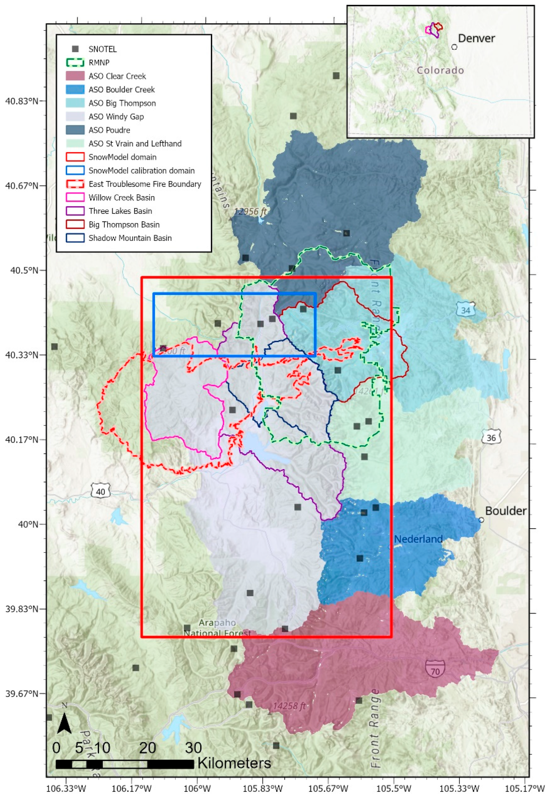
2.1. Study Area

The study area is a 78 km × 54 km (4212 km2) model domain in the north-central Colorado Rocky Mountains, US, ranging in elevation from 2278 m to 4345 m above sea level (Figure 1). The study area encompasses the headwaters of the Upper Colorado, North Platte, and South Platte River Basins. The land cover of the study area is composed of approximately 17% bare rock and alpine tundra area above treeline, 66% forested area, and 17% non-forested area below treeline [43]. The East Troublesome Fire was a large wildfire (784 km2) that occurred within parts of the study area between October and November 2020 (Figure 1; [44]). The study area is positioned within a snow-dominated mountainous region that accumulates deep seasonal snowpacks, and the year-to-year variability in streamflow is mainly driven by snowpack water storage and subsequent snowmelt [2].

2.2. Model Description and Simulations

To simulate detailed snow evolution processes across the study area, we utilized SnowModel, a spatially distributed, time-evolving, physically based snow modeling system designed for application in a wide range of environments where snow occurs (Figure 2; [47,48,49]). SnowModel includes the following submodels: MicroMet [50], a high-resolution meteorological distribution model; EnBal [51], a model of surface energy exchange between the snow and atmosphere; SnowPack [52], a seasonal evolution model of snow depth, snow density, and SWE; SnowTran-3D [53,54], a three-dimensional model of snow redistribution by wind across topographically variable terrain; and SnowAssim [55], a data assimilation system used for assimilating observations into SnowModel. SnowModel includes the physics required to simulate all first-order processes governing the seasonal evolution of a snowpack, including blowing snow redistribution and snow sublimation [15,48]. SnowModel has been shown to perform well in seasonally snow-covered environments within and similar to the study area (e.g., [8,15,30,56,57,58]).
SnowModel simulations were run at a 3-hourly time step with a 30 m spatial grid resolution for water years (from 1 October to 31 September) 2000 through 2023. Elevation, canopy cover fraction, and land cover for the model domain were provided by the U.S. Geological Survey (USGS) National Elevation Dataset [60], USGS National Land Cover Database [61], and the National Park Service (NPS) Vegetation Mapping Inventory Project for Rocky Mountain National Park ([62]; Supporting Information S1), respectively. Effective leaf area index (LAI*) values across the domain were generated by scaling the maximum LAI* for each forest class vegetation type by the canopy cover fraction (e.g., [15,58]). The LAI* for burned forest areas were adjusted based on the methods described in Sexstone et al. [58]. Furthermore, this study used the snow albedo decay parameterization to represent snow albedo decay in non-forested, forested, and burned forest areas for both non-melting and melting snow conditions presented by Sexstone et al. [58]. Meteorological forcing data for the SnowModel simulations were provided by the 1/16° grid-spacing near-real-time North American Land Data Assimilation System (NLDAS-2) reanalysis forcing dataset [63]. NLDAS-2 was used for this study as it provides (1) the sub-daily forcing variables that are required to run SnowModel, (2) the historical record needed for model calibration, and (3) the relatively low latency needed to run the model in near real time (latency of 5 days). Hourly NLDAS-2 forcing data were aggregated into 3-hourly values to correspond with the model simulation time step. The 3-hourly NLDAS-2 forcing data, along with mean elevation of each NLDAS-2 grid cell, were used by MicroMet to downscale and create the 30 m spatial resolution meteorological forcing data required by SnowModel [50].
This study implemented five primary configurations of SnowModel to evaluate differences and possible improvements in model performance (Table 1). The first configuration used the default SnowModel parameters without use of data assimilation (SnowModeldefault_noassim). The SnowAssim data assimilation system was used in subsequent configurations of SnowModel in this study to assimilate daily SWE values from 17 long-term SNOTEL stations across the study domain [55]. This data assimilation procedure used comparisons between daily SWE values from each SNOTEL station to daily simulate SWE to generate precipitation and melt rate adjustment factors for each year of the simulation period that were spatially interpolated across the domain [55]. The default SnowModel parameters (with data assimilation) were also used for the second model configuration (SnowModeldefault). The third and fourth configurations of SnowModel included the calibration of SnowModel parameters (SnowModelcalibrated) and the addition of a Landsat-based precipitation correction field (SnowModelLandsat), and are described in Section 2.3. Lastly, a post-processing routine to update calibrated SnowModel gridded outputs using remotely sensed SCA images was developed (SnowModelSCA_update), and is described in Section 2.4.

2.3. Model Calibration

A calibration subdomain (32 km × 13 km) containing 5 SNOTEL stations was developed within the study area for calibrating SnowModel (SnowModelcalibrated; Figure 1) to make running time manageable. The calibration subdomain showed an elevational (median elevation of 3196 m; Figure S1) and land cover (68 percent forest cover) distribution that was comparable to the entire study domain (median elevation of 2967 m, 66 percent forest cover). We used a single-gridded representation of Landsat-derived mean annual snow persistence (SP; the average number of days per year that a grid cell is snow-covered between January and July; Supporting Information S2) and time-series gridded data of cloud-gap-filled [64] MODIS (MOD10A1F) and VIIRS (VNP10A1F) snow-covered area (SCA; ratio of snow-covered area to total area) as the primary spatial and temporal calibration targets, respectively. Both the mean annual historical Landsat dataset and the daily cloud-gap-filled MODIS and VIIRS datasets used in this study helped address possible limitations of these observations from revisit cycles and cloud cover. This multi-objective calibration approach using remotely sensed SP and SCA reduced the dependence on SNOTEL SWE observations for model validation and allowed for these ground-based SWE measurements to be assimilated into SnowModel to adjust rates of snow accumulation and melt. However, snow density observations from SNOTEL stations were additionally used as a model calibration target. The spatial efficiency metric (SPAEF), a multiple-component (correlation, coefficient of variation, and histogram overlap) evaluation metric of spatial patterns [65], was used to compare spatial patterns of SnowModel and Landsat SP. Root mean squared error (RMSE) and Nash–Sutcliffe efficiency (NSE) objective functions were used to compare MODIS/VIIRS and SnowModel daily mean SCA, as well as SNOTEL snow density and SnowModel snow density across the calibration domain. A range of SnowModel parameters that define snow density evolution, wind redistribution of snow, and snow albedo were calibrated using Latin hypercube sampling [66] in a stepwise process (Table 2). Parameter ranges were determined by previous studies (e.g., [47,58]) and expert opinion to effectively explore the parameter space. We ran 600 different uniquely parameterized SnowModel simulations on the USGS Denali Supercomputer [67] in parallel for water years 2000 through 2020. The parameter sets that maximized SPAEF and NSE and minimized RMSE were considered for the final calibrated parameters. However, parameter sets that maximized Landsat SPAEF did not always minimize MODIS RMSE; therefore, final preference was given to the parameter set that optimized the SPAEF metric in the calibration subdomain as it also resulted in a comparatively low MODIS RMSE.
Subsequently, as part of the calibration effort, a grid-by-grid Landsat-based precipitation correction field was developed and applied to SnowModelcalibrated simulations to further adjust the calibrated model for biases in the meteorological forcing data (SnowModelLandsat). This precipitation correction field was developed according to the exponential relation between SP and peak SWE for all SNOTEL stations within the study domain (Figure 3). For each SNOTEL station, the mean annual SP and mean annual peak SWE were computed for water years 2000 through 2020. The normalized difference in SP (SP minus mean annual SP) and the normalized ratio of peak SWE to mean annual peak SWE were then computed by site for each water year. The normalized difference in SP was then plotted against the normalized ratio of peak SWE to mean peak SWE for all SNOTEL sites within the study area (Figure 3). This exponential relation was then used to convert the grid-by-grid difference in mean annual SP between SnowModelcalibrated and Landsat to the grid-by-grid Landsat-based precipitation correction field for the model domain. The Landsat-based precipitation correction field was applied to all SnowModelLandsat simulations.

2.4. SnowModel Output Grid Updates Using Remotely Sensed SCA

This study also developed a post-processing routine for SnowModel output grids to be updated with fine-resolution remotely sensed SCA data (e.g., Landsat, Sentinel-2) in support of additional real-time model applications (SnowModelSCA_update). SnowModel output grids with SWE greater than 10 millimeters (mm) were considered as snow covered [68] and compared to overlapping remotely sensed SCA for this study. For scenarios when SnowModel output grid SCA and remotely sensed SCA did not differ, no updates to the SnowModel output grids were made. For scenarios when a SnowModel output grid was simulated as snow covered but the remote sensing observation showed the grid as snow free, the SnowModel output grid SWE for that grid cell was set to 0 mm. For scenarios when a SnowModel output grid was simulated as snow free but the remote sensing observation showed the grid as snow covered, the SnowModel output grid was updated with an elevation and aspect-based mean SnowModel SWE output condition computed for each basin of interest. This mean SnowModel SWE output was computed from output grid SWE values greater than 0 mm for 200 m elevation zones within north-facing, east-facing, south-facing, and west-facing aspects (Figure 2). In this study, SnowModelSCA_update (SnowModelLandsat output grids updated with remotely sensed SCA) outputs were generated only for dates that corresponded with remotely sensed SCA images.

2.5. Model Evaluation

The SnowModel simulations developed for this study (Table 1) were evaluated by airborne lidar-derived SWE (observed snow depth and modeled snow density) datasets generated by ASO [41] during April and May 2022 and 2023 for the Colorado River at Windy Gap and Big Thompson River Basins (Figure 1). ASO SWE datasets (50 m spatial resolution) were resampled to the SnowModel grid resolution (30 m spatial resolution) using bilinear interpolation. Comparisons of mean SWEs from ASO and SnowModel were made at the basin scale and by elevation zones that are commonly used for streamflow forecasts in this region (high elevations [>3124 m], middle elevations [2438–3124 m], and low elevations [<2438 m]) within the study area. Additionally, a grid-by-grid evaluation of ASO datasets and SnowModel was used to evaluate mean error, mean absolute error, RMSE, percent bias, NSE, and Pearson correlation coefficient performance metrics for the SnowModel versions developed in this study. These comparisons and statistics included areas with zero or very low snow; thus, evaluations across elevation zones allowed for an assessment over a range of observed SWE values. Model evaluation results were compared between the SnowModeldefault_noassim, SnowModeldefault, SnowModelcalibrated, and SnowModelLandsat configurations.
Comparisons of model performance between the SnowModelLandsat and SnowModelSCA_update (SnowModelLandsat updated with remotely sensed SCA) were also made to evaluate the value added from using remotely sensed SCA in near-real-time SnowModel applications. In this study, ASO remote sensing datasets were classified as snow covered if the ASO-derived SWE was greater than 10 mm. Landsat fractional SCA remote sensing datasets were considered as snow covered if fractional SCA was greater than 10 percent [69]. In the first step of this analysis, we used three ASO datasets collected in late May for the Shadow Mountain Basin (26 May 2022, 27 May 2023) and the Big Thompson Basin (21 May 2023) to generate SnowModelSCA_update gridded outputs and evaluate model performance. The ASO remotely sensed datasets were used to (1) compute the observed SCA, (2) update the SnowModel simulations based on these SCA observations, and (3) evaluate modeled SWE performance. For a second assessment of SnowModelLandsat and SnowModelSCA_update outputs, we used a time series from the Landsat fractional SCA images [70,71] for observations of SCA. We evaluated the differences between SnowModelLandsat and SnowModelSCA_update outputs throughout the snow season from January through August 2010 to 2012 and 2018 to 2020 for the Shadow Mountain Basin. Landsat SCA images were only used to generate SnowModelSCA_update outputs during this period when there were less than 25% missing observations because of cloud cover.
Table 2. SnowModel parameters with default and final calibrated values and the ranges for each parameter that were used for the Latin hypercube sampling [43].
Parameter Description (Parameter Name)Calibration Step and ProcessDefault ValueCalibrated Value [Calibration Range]
Rain–snow threshold (snowfall_frac)not calibrated[72][72]
Snow density rate adjustment factor (ro_adjust)step 1: snow density evolution5.00.4 [0.1–5.0]
Curvature length scale (curve_len_scale)step 2: wind redistribution of snow500575 [30–600]
Slope weight factor (slopewt)step 2: wind redistribution of snow0.580.18 [0, 1]
Curvature weight factor (curvewt)step 2: wind redistribution of snow0.420.82 [0, 1]
Wind increase/decrease with elevation (wind_lapse_rate)step 2: wind redistribution of snow0.01.81 [1, 2]
Forest snow albedo minimum (for_al_min)step 3: snow albedo0.400.22 [0.10–0.55]
Open area snow albedo minimum (open_al_min)step 3: snow albedo0.500.42 [0.10–0.55]
Forest snow albedo maximum (for_al_max)step 3: snow albedo0.680.56 [0.55–0.90]
Open area snow albedo maximum (open_al_max)step 3: snow albedo0.800.71 [0.55–0.90]
Forest snow albedo decay cold snow (for_al_gr_cold)step 3: snow albedo0.030.02 [0.010–0.035]
Open area snow albedo decay cold snow (open_al_gr_cold)step 3: snow albedo0.020.02 [0.010–0.035]
Forest snow albedo decay melting snow (for_al_gr_melt)step 3: snow albedo0.060.06 [0.045–0.095]

3. Results

3.1. Model Calibration

The SnowModel parameters calibrated for this study are shown in Table 2. Calibration parameter adjustments generally resulted in slower snow density increases with time, greater wind speeds and a resulting blowing snow redistribution and sublimation at high elevations, and lower snow albedos for both open and forested environments. SnowModelcalibrated showed a reduced RMSE for the snow density and SWE at the SNOTEL stations compared to SnowModeldefault_noassim (Table S1). An example of how the models’ performances regarding the simulated snow density at the SNOTEL stations varied with the snow density rate adjustment factor parameter is shown in Figure S2. A comparison of the SnowModel simulations to the MODIS observations for the time-series domain-wide SCA (percent of domain that is snow-covered) shows an improved RMSE, from 13.3% to 11.3%, during the calibration (Figure 4; Table S2). SnowModelcalibrated also shows an improved SPAEF, from 0.10 to 0.22, compared to SnowModeldefault (Figure 5; Table S2).
A Landsat-based precipitation correction field ranging from 0.1 to 2.5 based on the simulated versus observed mean annual SP was used as an additional step in the calibration process for this study (Figure 3 and Figure S3). The spatial field of the Landsat-based precipitation correction factors applied to the SnowModelLandsat simulations is shown in Figure S3. The Landsat-based correction field further improved SnowModelLandsat’s performance compared to SnowModelcalibrated’s on the SNOTEL (Table S1) and MODIS (Figure 4; Table S2) data comparisons. However, SnowModelLandsat had a lower overall SPAEF performance compared to SnowModelcalibrated when evaluating the spatial pattern of the Landsat SP (Figure 5; Table S2). Despite the decrease in the overall SPAEF, applying the correction field to the modeled precipitation substantially improved the overall correlation (α) between SnowModelLandsat and Landsat SP (Figure 5; Table S2). Additionally, the mean bias between SnowModelLandsat and Landsat SP (−2.8 days) was lower compared to the mean bias between SnowModelcalibrated and Landsat SP (−3.7 days; Figure 5). Although SnowModelLandsat was generally shown to improve the simulation of the SP, the low-elevation areas were generally biased toward lower values (Figure 5).

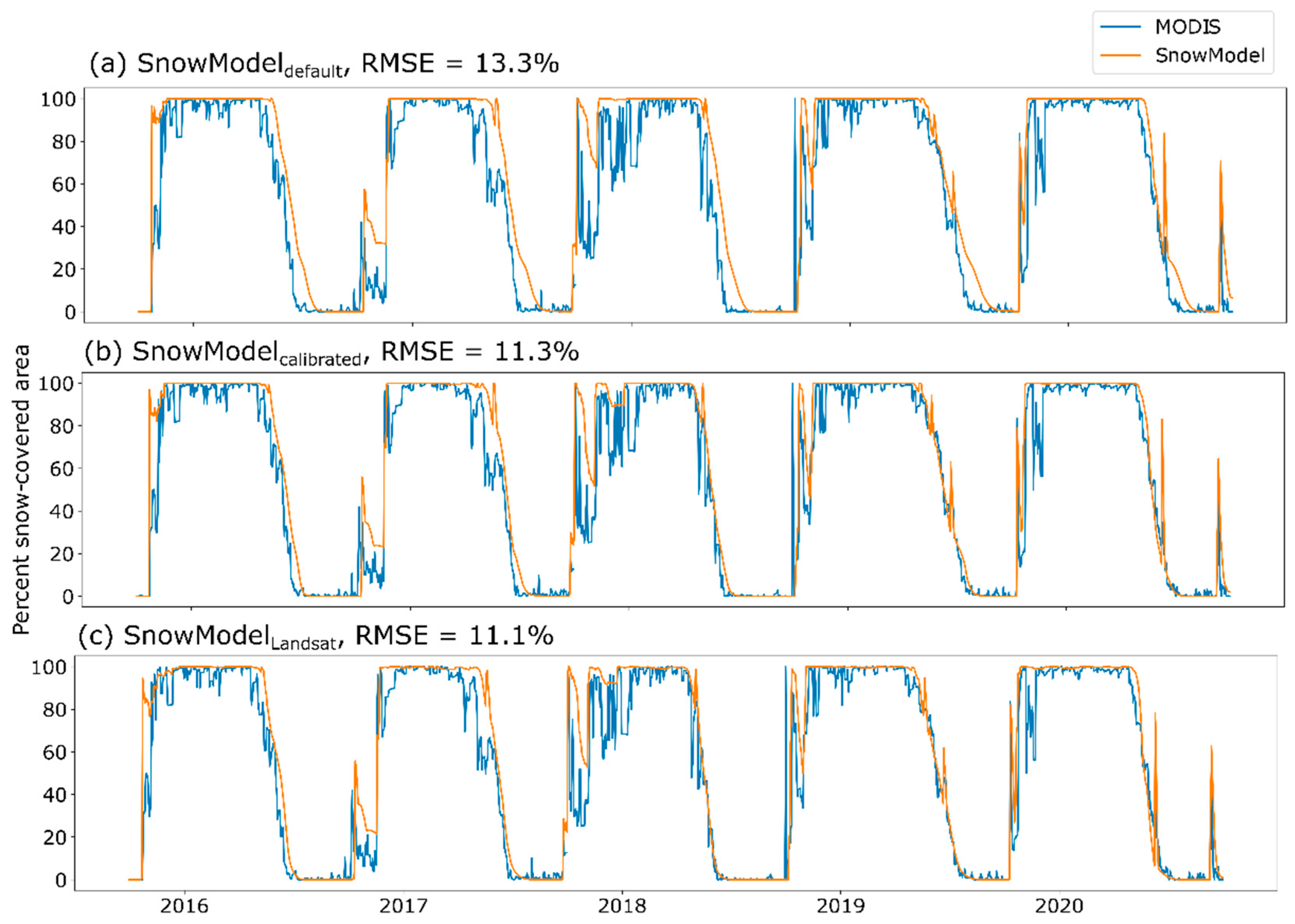
3.2. Model Comparisons with Historical Model

We evaluated the differences in the four SnowModel versions developed by this study (SnowModeldefault_noassim, SnowModeldefault, SnowModelcalibrated, and SnowModelLandsat), and compared these simulations with the SNOw Data Assimilation System (SNODAS) [27], a commonly used operational snow model available at a 1 km spatial grid resolution (Figure 6). For comparison, the SNODAS outputs were resampled to the 30 m SnowModel spatial resolution grid. The assimilation of the SNOTEL SWE data into SnowModeldefault resulted in substantial increases in the SWE compared with SnowModeldefault_noassim, especially at high elevations, where the peak SWE was approximately 1.75 times higher. The calibrated SnowModelcalibrated resulted in a reduction in the SWE at high elevations as a result of increased blowing snow redistribution and sublimation, as well as an earlier melt-out across all elevations compared to SnowModeldefault (Figure 6). SnowModelLandsat showed small increases or decreases in the SWE and more gradual and later melt-outs compared to the calibrated model for the middle and high elevations. Both SnowModelcalibrated and SnowModelLandsat simulated greater SWEs across all elevations (especially at high and low elevations) compared to the SNODAS model. The SNODAS model showed a more rapid snowmelt rate and earlier melt-out compared with SnowModel (Figure 6).

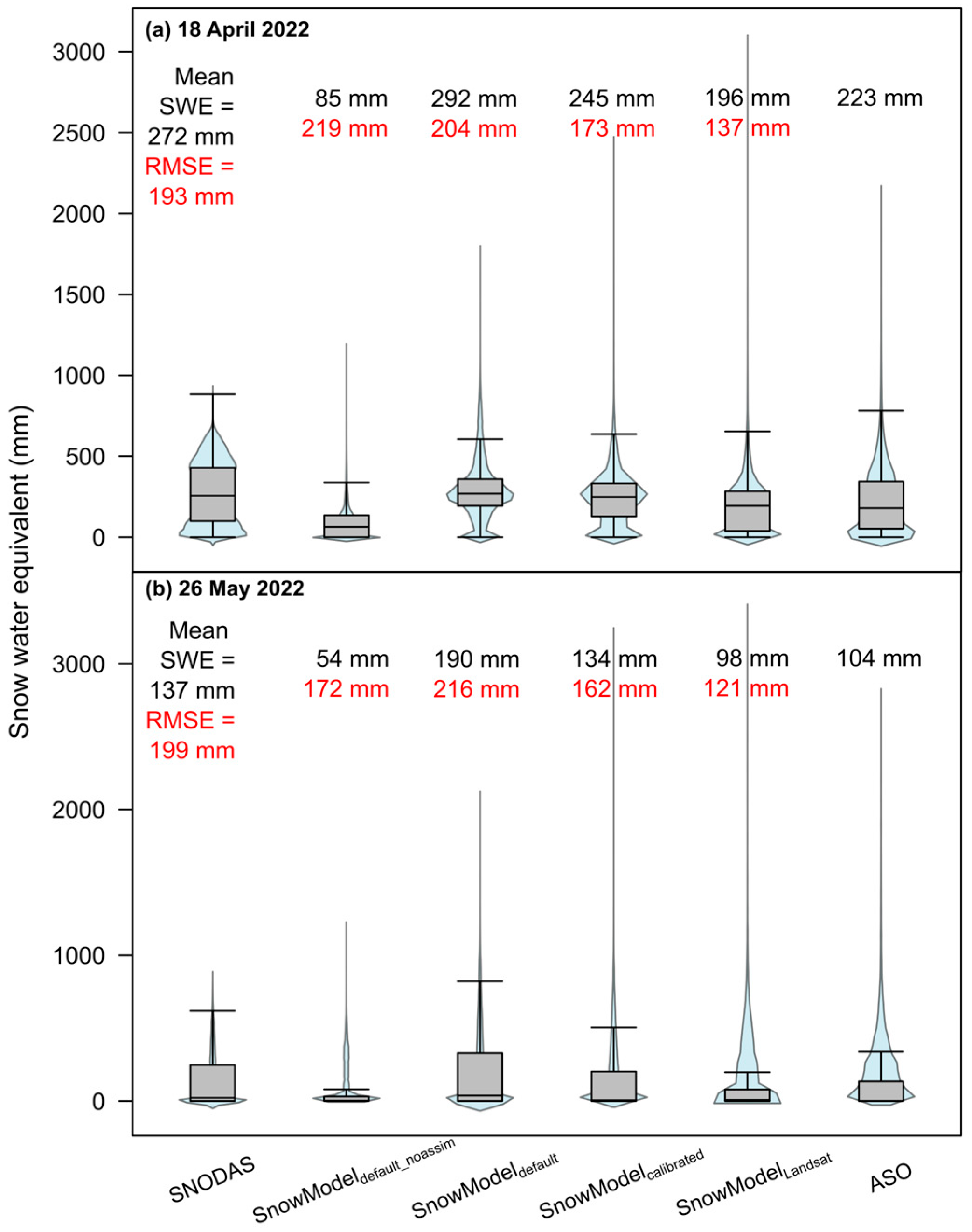
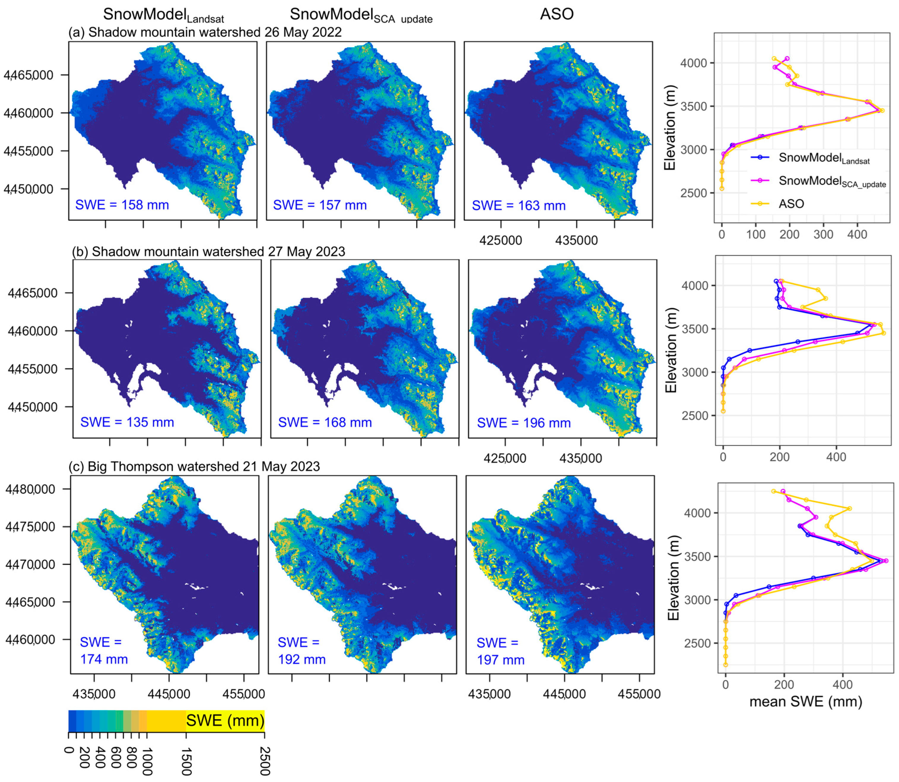
3.3. Model Evaluations Compared to ASO

On 18 April 2022 and 26 May 2022, ASO flights collected information for the Windy Gap Basin (Figure 1). Comparisons between the ASO-derived SWE, SNODAS SWE, and the four SnowModel versions developed by this study (Figure 7) show the improved performance of the SnowModelcalibrated (mean error ranging from 22 to 31 mm) and SnowModelLandsat (mean error ranging from −28 to −6 mm) versions compared to the SNODAS (mean error ranging from 34 to 48 mm) and SnowModeldefault (mean error ranging from 69 to 86 mm). The results indicate a negative bias in SnowModeldefault_noassim and a positive bias in SnowModeldefault, highlighting the influence of assimilating the SNOTEL SWE data into the default model (Figure 7 and Figure 8). Additionally, SnowModelLandsat showed improved error and correlation performance metrics compared to SnowModelcalibrated (Table 3 and Table S3). SnowModelLandsat’s simulated basin-wide mean SWE (196 mm, 98 mm) compared well to the ASO SWE estimates (223 mm, 104 mm) for 18 April 2022 and 26 May 2022, respectively (Figure 7). The mean difference between the SnowModel SWE and ASO-derived SWE across the basin on 26 May 2022 was only −6 mm (Table S3), and the spatial patterns of the datasets were well correlated (Table S3; Figure 8). The observed errors were somewhat homogenous spatially from north to south (Figure 8d), which may indicate interannual differences in the snow accumulation patterns compared to the mean annual conditions. Both the SNODAS and SnowModelLandsat performed relatively well at simulating the mean SWE conditions across all elevation zones (Table 3 and Table S3). However, a grid-by-grid comparison of the SnowModelLandsat and ASO-derived SWE (RMSE of 137 mm and 121 mm for 18 April 2022 and 26 May 2022, respectively) showed a substantial improvement compared to the comparison of the SNODAS and ASO-derived SWE (RMSE of 193 mm and 199 mm for 18 April 2022 and 26 May 2022, respectively) across the middle and high elevation zones (Figure 7, Table 3).

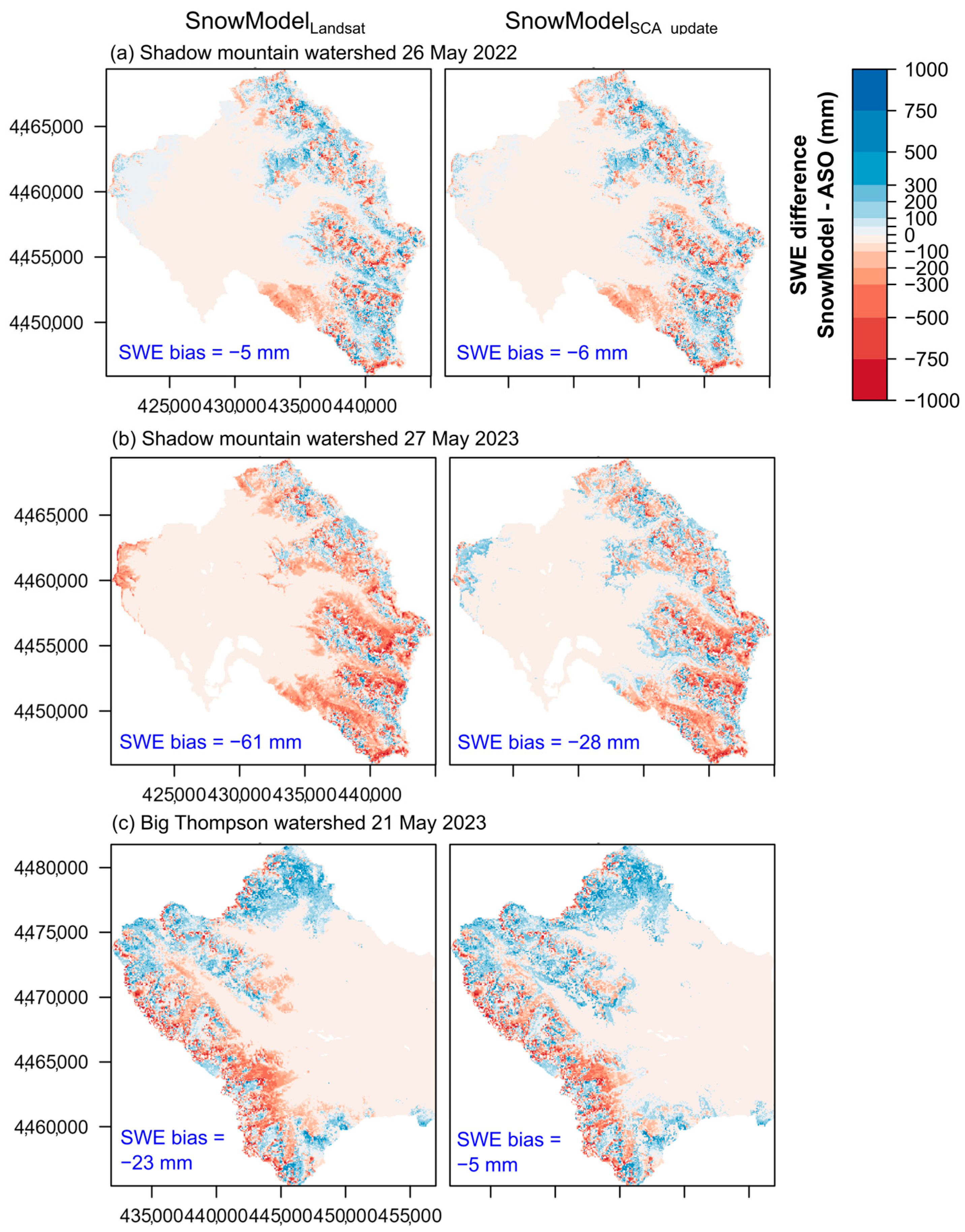
3.4. Value Added Using Additional Real-Time Remote Sensing Datasets

We evaluated whether the SnowModelLandsat simulations could be further improved using remotely sensed SCA observations in a real-time framework. The mean bias of the SnowModelLandsat simulation compared to that of the ASO for the Shadow Mountain Basin for 26 May 2022 was very small (−5 mm), and further model improvements from updating the SnowModel output with the ASO SCA observations (SnowModelSCA_update) were not shown (Figure 9 and Figure 10). However, a larger negative bias in the SnowModelLandsat simulations was observed for the Shadow Mountain Basin on 27 May 2023 and the Big Thompson Basin on 21 May 2023; the SnowModelSCA_update simulations further reduced these mean biases from −61 mm to −28 mm and from −23 mm to −5 mm, respectively (Figure 9 and Figure 10). For all three dates evaluated, the greatest reductions in bias were found for the middle elevation zones between 3000 m and 3300 m, which were slightly above the snow line during that time of year (Figure 9 and Figure 10).
The Landsat fractional SCA data [70,71] for the Shadow Mountain Basin, from January through August 2010 to 2012 and 2018 to 2020, included 31 percent (n = 67) of images with less than 25 percent missing grid cells because of cloud cover. Comparisons between SnowModelLandsat and SnowModelSCA_update using this time series of images showed that the mean absolute difference across all the images for the basin was small (7 mm; Figure 11). However, the mean differences between the model versions for the basin were as large as −82 mm. The percentage difference between SnowModelLandsat and SnowModelSCA_update was generally greater than 5% during January, May, June, July, and August, indicating that this technique is likely most useful during the early accumulation and snowmelt seasons (Figure 11).

4. Discussion

4.1. Advantages of Near-Real-Time Spatially Distributed Snow Modeling Approach

The key results of this study highlight that information from fine-spatial-resolution (30 m) and high-temporal-resolution (daily) remotely sensed snow cover can support important improvements to process-based snow modeling simulations that can be run in near real time. In complex mountainous environments, the patterns of mean annual SP that have been observed by Landsat highlight important repeatable snow-holding patterns across these landscapes [73], and this information was used as a valuable spatial calibration target for the snow modeling performed in this study (Figure 5). A time series of domain-wide MODIS/VIIRS daily SCA observations was also used as an important temporal calibration target that was particularly important for better representing the snowmelt timing (Figure 4). Furthermore, our results show that the strong relation between the SP and peak SWE [69,74,75] can be leveraged to further constrain and bias-correct the precipitation forcing patterns for process-based snow modeling (Figure 7 and Figure 8). This result is consistent with the many studies that have highlighted how the snow patterns across these landscapes tend to be temporally consistent from year to year [76,77,78,79,80]. The results from this study also highlight that post-processing of the SnowModel gridded outputs with observed fine-resolution SCA (e.g., from Landsat or Sentinel 2) can further refine process-based snow model SWE estimates; these updates are shown to have the greatest influence on SWE estimates (Figure 9 and Figure 11) at or near snow-line elevations during the early accumulation and late snowmelt seasons [32,81]. Taken together, these results present a new approach for calibrating and post-processing a process-based snow model that can be applied in near real time using fine-spatial-resolution and high-temporal-resolution remotely sensed snow cover information.
Process-based snow modeling at fine spatial resolutions using the approach outlined in this study has important advantages for the development of additional near-real-time SWE estimations. This modeling approach includes the first-order processes governing the seasonal evolution of snowpacks that could be able to represent varying sensitivities to future climate-induced changes to snowpacks’ energy balance [8,82,83,84]. Furthermore, the fine spatial resolution of the model grid allows for a more realistic representation of the topographic influences on the snow process dynamics [85,86]. The SnowModel simulations developed in this study importantly capture the complex snow patterns (Figure 9) and the more gradual snowmelt rate (Figure 6) at the highest elevations. These snow dynamics are driven by deep pockets of wind-redistributed snow and are more accurately simulated here because of the incorporation of remotely sensed snow cover data into the model’s development. The comparison of high-elevation SWE shown in Figure 6a and Figure 8 highlights the contrast between the rapid depletion of snow simulated by the coarser SNODAS model with the more gradual late-season snowmelt simulated by SnowModelLandsat. Its more accurate quantification of late-season high-elevation snow water storage and variability (Table 3) and snowmelt runoff could be important for the management of inflow forecasts for reservoirs in high-elevation basins. The near-real-time modeling approach presented in this study fills an important need and can support additional snow and water supply forecasting, and can be applied with available fine-resolution remote sensing datasets [87,88] anywhere on earth.

4.2. Comparisons to Previous Investigations

To put the results of this study in the context of previous investigations, we compared the model performance statistics for the model developed in this work to other SWE estimation studies that have compared their results to the ASO datasets. SnowModel simulations calibrated for the Rio Grande headwaters [58] at a 100 m spatial resolution showed a grid-by-grid RMSE of 159 mm when compared to an ASO flight around peak snow accumulation. The results presented in this study show comparable but improved performance statistics to those of Sexstone et al. [58], with comparisons to the ASO highlighting RMSE values from 121 to 137 mm (Table S3). Other recent process-based modeling studies have also presented comparisons to the ASO, but have focused their results on comparisons of the snow depth rather than SWE [40,89]. Bair et al. [90] developed two reconstruction models for basins in the Sierra Nevada, California, that compared favorably with the ASO (25 and 26 mm mean absolute error). Furthermore, Yang et al. [24] developed a retrospective model combined with additional statistical techniques in the same study area to develop a real-time SWE estimation approach; the results from that study highlighted a median RMSE of 133 mm from comparisons with the ASO. Importantly, the results from Bair et al. [90] and Yang et al. [24] were presented based on a 500 m spatial resolution. However, they are still generally comparable to the performance statistics presented by this study. Dawson et al. [91] compared the results from a 4 km spatial resolution University of Arizona SWE product [92] to ASO data averaged across the basin scale in California and found a mean absolute error of 52 mm. When computed based on a 30 m grid comparison, the results from this study show a mean absolute error ranging from 54 to 87 mm. However, when averaged at the basin scale, the mean absolute error from two flight comparisons is 17 mm (Table S3).

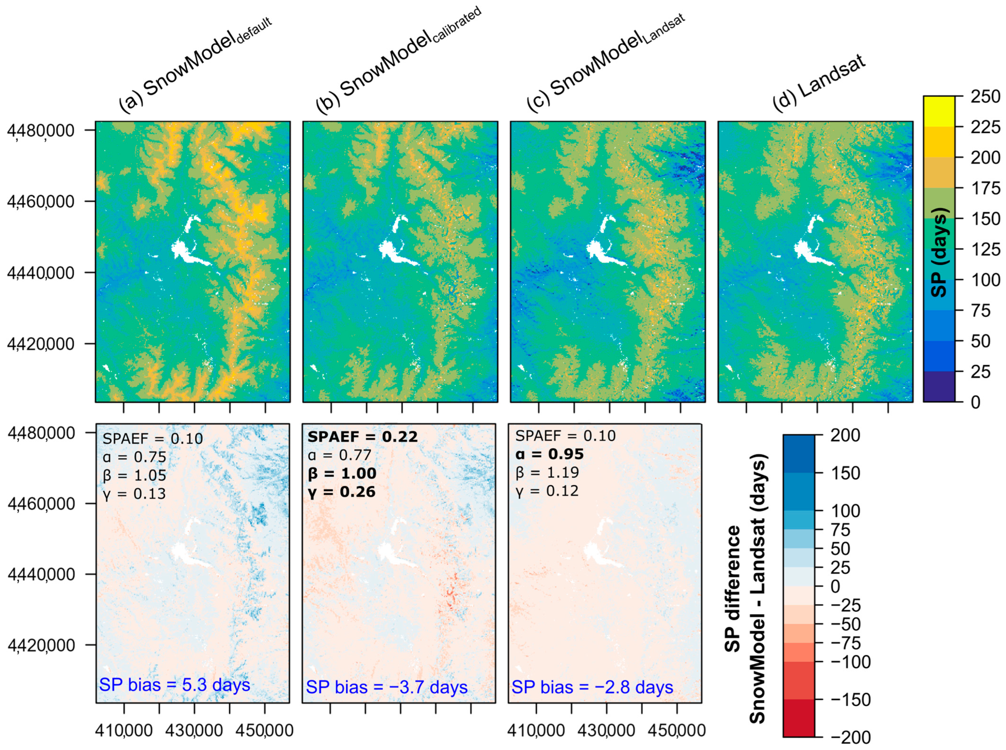
4.3. Temporal Consistency of Snow Patterns

This study implemented a spatial precipitation correction field in the model simulations that builds off previous research highlighting how the temporal consistency of snow patterns across a landscape can be used to improve snow estimates. The data assimilation scheme SnowAssim [55], developed for SnowModel, was built on the premise that observations of snow can be used to help reduce the model uncertainty associated with biases in model forcing (e.g., precipitation, wind) or process representation (e.g., blowing snow redistribution). Sturm and Wagner [76] used empirically derived snow distribution patterns derived from repeated snow surveys to improve SnowModel simulations by up to 60%. Additionally, Vögeli et al. [77] used maps of snow depth distributions from digital photogrammetry to scale the precipitation input data for the Alpine3D snow model [93], showing a reduction in the snow depth error by a factor of 3.4. Recent work has also highlighted that snow patterns derived from historical aerial lidar snow depth surveys can be used to accurately infer snow depth patterns and snow deposition downscaling [78,94], although important challenges have been highlighted, associated with seasons exhibiting abnormal snow accumulation, mid-winter ablation, and snowmelt conditions. Despite the overall improvements in the SnowModelLandsat simulations using the Landsat SP pattern correction field in this study, we highlight that the errors using this approach are spatially homogenous (Figure 8d), which may indicate similar challenges associated with interannual differences in snow accumulation patterns. Previous research has mainly used measurements of the SWE or snow depth to evaluate spatial corrections of snow distributions in process-based snow modeling. However, similar to Hammond et al. [74] and Trujillo and Molotch [75], we show that the SP is well correlated with the peak SWE, and we developed a relation between the SP and peak SWE (Figure 3) that was used to scale the precipitation inputs into the SnowModel based on a similar approach presented by Vögeli et al. [77] and Raleigh and Deems [37] that was able to further reduce the SnowModel RMSE by 36–41 mm from the calibrated model version (Table S3). As noted by Wayand et al. [73], patterns of SP from fine-resolution SCA are globally scalable. Therefore, additional research that evaluates how the relation between the SP and peak SWE varies across different snow regimes [75], and that could support linkages between SP and SWE patterns to improve process-based snow modeling and downscaling, would be useful.

4.4. Uncertainties and Future Research

Major uncertainties in process-based snow modeling are often associated with the uncertainties in atmospheric forcing datasets [38]. In this study, we observed a low bias in the precipitation and wind speeds from the NLDAS-2 forcing data, which has been similarly observed by previous studies [95,96]. The calibration, precipitation scaling, and data assimilation model results developed in this study are, importantly, specific to the atmospheric forcing dataset used (NLDAS-2 in this application) and its inherent biases. However, the peak SWE and SP relation used for precipitation scaling is likely transferable because it is solely based on observations. The approaches developed in the model workflow attempt to reduce forcing-based model uncertainties. Therefore, if major changes were made to the atmospheric forcing dataset, or a different atmospheric forcing dataset was used in the future, the model calibration and precipitation correction field would need to be redeveloped specifically to the new forcing dataset. Future research testing the model workflow developed by this study using a range of atmospheric forcing datasets could provide important information about the consistency between forcing-based and model process-based uncertainties. Additionally, future improvements in the spatial resolution, accuracy, and latency of atmospheric forcing datasets and, similarly, improvements in the spatial resolution and revisit cycles of remotely sensed snow cover products could be utilized in future process-based snow modeling applications with the modeling workflow presented by this study.
This study used the ASO SWE estimates as the primary evaluation dataset for the SnowModel results, and it is shown that the majority of the uncertainty in the lidar-derived SWE estimation techniques is associated with snowpack density modeling [97]. However, the magnitude of the ASO product’s SWE uncertainty is far less than other SWE estimation techniques presented by other studies [41]. Evaluating the differences between the ASO and SnowModel snow density modeling approaches was outside of the scope of this research, but future research evaluating the differences and uncertainties in process-based snow modeling of snow density and their importance in real-time snow estimation could be explored.
Future research could build upon the SnowModel calibration procedure that is developed in this study. Process-based snow models, such as SnowModel, are not typically calibrated using automated methods given the computational expense of this process and the relatively good model performance without these procedures (e.g., [8,15,30,56,57,58]). However, this study highlights how automated calibration procedures can improve the SnowModel’s performance from the baseline conditions (Figure 8, Table S3). The use of a single calibration subdomain in this study may have limited the generalizability of the model; thus, future research could consider how to use a greater number of calibration subdomains across a similarly large study area. Additionally, we suggest that future research could conduct a sensitivity analysis of the calibrated parameters to better understand the significance of each of the calibrated parameters within the calibration process. Lastly, as more airborne lidar-derived snow products become available, future research could analyze the robustness of this type of calibration method over several years in varying climate conditions.

5. Conclusions

The SnowModel simulations were developed over a 24-year period (2000–2023) at a 30 m spatial grid resolution across a 4212 km2 model domain in the north-central Colorado Rocky Mountains. An NLDAS-2 reanalysis was utilized for the model’s atmospheric forcing data, and the SNOTEL SWE observations were incorporated via data assimilation. The SnowModel was calibrated spatially to the Landsat mean annual SP and temporally to the MODIS/VIIRS mean basin SCA using a multi-objective calibration procedure performed through Latin hypercube sampling and a stepwise calibration process. The Landsat mean annual SP was also used to further optimize the SnowModel simulations through the development of a spatially variable precipitation correction field. This study additionally developed a near-real-time workflow for the SnowModel simulations that includes post-processing corrections of the model outputs using observed fine-resolution SCA information. The evaluations of the SnowModel simulations using lidar-derived ASO SWE estimates highlight that the version of SnowModel calibrated to the remotely sensed SCA had an improved performance compared with the baseline simulations and comparable spatial patterns to that of the ASO, especially at the highest elevations. Grid-by-grid comparisons of the baseline and final calibrated SnowModel simulations to the ASO-derived SWE showed an improvement in the mean RMSE from 210 mm to 129 mm, respectively. Furthermore, the post-processing corrections of the SnowModel gridded outputs using the observed fine-resolution SCA were shown to further improve the model’s accuracy, having the greatest influence on the SWE estimates at or near snow-line elevations during the early accumulation and late snowmelt seasons. The results presented in this study highlight a new approach that can be used for calibrating and post-processing a process-based snow model and can be applied in near real time using fine-resolution snow cover information. This research has the potential to informing additional assessments, management planning, and water resources forecasting by providing improvements in near-real-time to snow water storage estimates within seasonally snow-covered mountainous environments.

Supplementary Materials

The following supporting information can be downloaded at: https://www.mdpi.com/article/10.3390/rs17101704/s1, Reference [98] is cited in Supplementary Materials.

Author Contributions

Conceptualization, G.A.S., D.J.S., C.L.-S. and E.C.; methodology G.A.S., G.A.A., D.J.S. and T.B.B.; software, G.A.S., G.A.A. and T.B.B.; validation, G.A.S., G.A.A. and D.J.S.; formal analysis, G.A.S., G.A.A., D.J.S. and T.B.B.; investigation, G.A.S., G.A.A., D.J.S., T.B.B., D.M.R., C.L.-S., E.C. and L.A.B.; resources, G.A.S., G.A.A., D.J.S., T.B.B., D.M.R., C.L.-S., E.C. and L.A.B.; data curation, G.A.S., G.A.A., D.J.S., T.B.B. and D.M.R.; writing—original draft preparation, G.A.S., G.A.A., D.J.S., T.B.B., D.M.R., C.L.-S., E.C. and L.A.B.; writing—review and editing, G.A.S., G.A.A., D.J.S., T.B.B., D.M.R., C.L.-S., E.C. and L.A.B.; visualization, G.A.S., G.A.A., D.J.S., T.B.B. and D.M.R.; supervision, G.A.S., C.L.-S. and E.C.; project administration, G.A.S., C.L.-S., E.C. and L.A.B.; funding acquisition, G.A.S., D.J.S., C.L.-S. and E.C. All authors have read and agreed to the published version of the manuscript.

Funding

This research was funded by the Bureau of Reclamation Science and Technology Program, the Snow Water Supply Forecast Program, and by the Northern Colorado Water Conservancy District (Northern Water). Additional funding support was provided by the U.S. Geological Survey (USGS) Water Availability and Use Science Program as part of the Water Resources Mission Area Snow Hydrology Research Project and the USGS Ecosystems Land Change Science Program. Funding for the Airborne Snow Observatories (ASO) data collection within the Windy Gap domain used in this study was provided by the USGS Next Generation Water Observing System (NGWOS) Program and by Northern Water.

Data Availability Statement

The SnowModel output, land cover grids, and DEM used in this analysis are available via Akie et al. [43] and from the publicly available sources cited in the text. The Airborne Snow Observatories’ (ASO’s) datasets are also openly available [46].

Acknowledgments

The computing resources were provided by the USGS Core Science Systems Advanced Research Computing Center on the Denali and Tallgrass supercomputers [67]. We would like to thank Glen Liston for providing the SnowModel code used in this study [49]. Any use of trade, firm, or product names is for descriptive purposes only and does not imply endorsement by the U.S. Government.

Conflicts of Interest

The authors declare no conflicts of interest.

References

  1. Li, D.; Wrzesien, M.L.; Durand, M.; Adam, J.; Lettenmaier, D.P. How much runoff originates as snow in the western United States, and how will that change in the future? Geophys. Res. Lett. 2017, 44, 6163–6172. [Google Scholar] [CrossRef]
  2. Lukas, J.; Payton, E. Colorado River Basin Climate and Hydrology: State of the Science, Western Water Assessment; University of Colorado Boulder: Boulder, CO, USA, 2020. [Google Scholar] [CrossRef]
  3. Barnett, T.P.; Adam, J.C.; Lettenmaier, D.P. Potential impacts of a warming climate on water availability in snow-dominated regions. Nature 2005, 438, 303–309. [Google Scholar] [CrossRef]
  4. Pagano, T.; Garen, D.; Sorooshian, S. Evaluation of Official Western U.S. Seasonal Water Supply Outlooks, 1922–2002. J. Hydrometeorol. 2004, 5, 896–909. [Google Scholar] [CrossRef]
  5. Wheeler, K.G.; Udall, B.; Wang, J.; Kuhn, E.; Salehabadi, H.; Schmidt, J.C. What will it take to stabilize the Colorado River? Science 2022, 377, 373–375. [Google Scholar] [CrossRef] [PubMed]
  6. Richter, B.D.; Lamsal, G.; Marston, L.; Dhakal, S.; Sangha, L.S.; Rushforth, R.R.; Wei, D.Y.; Ruddell, B.L.; Davis, K.F.; Hernandez-Cruz, A.; et al. New water accounting reveals why the Colorado River no longer reaches the sea. Commun. Earth Environ. 2024, 5, 134. [Google Scholar] [CrossRef]
  7. Bales, R.C.; Molotch, N.P.; Painter, T.H.; Dettinger, M.D.; Rice, R.; Dozier, J. Mountain hydrology of the western United States. Water Resour. Res. 2006, 42, W08432. [Google Scholar] [CrossRef]
  8. Hammond, J.C.; Sexstone, G.A.; Putman, A.L.; Barnhart, T.B.; Rey, D.M.; Driscoll, J.M.; Liston, G.E.; Rasmussen, K.L.; McGrath, D.; Fassnacht, S.R.; et al. High Resolution SnowModel Simulations Reveal Future Elevation-Dependent Snow Loss and Earlier, Flashier Surface Water Input for the Upper Colorado River Basin. Earth’s Future 2023, 11, e2022EF003092. [Google Scholar] [CrossRef]
  9. Fassnacht, S.R.; Venable, N.B.H.; McGrath, D.; Patterson, G.G. Sub-Seasonal Snowpack Trends in the Rocky Mountain National Park Area, Colorado, USA. Water 2018, 10, 562. [Google Scholar] [CrossRef]
  10. Mote, P.W.; Li, S.H.; Lettenmaier, D.P.; Xiao, M.; Engel, R. Dramatic declines in snowpack in the western US. Npj Clim. Atmos. Sci. 2018, 1, 2. [Google Scholar] [CrossRef]
  11. López-Moreno, J.I.; Revuelto, J.; Fassnacht, S.R.; Azorín-Molina, C.; Vicente-Serrano, S.M.; Morán-Tejeda, E.; Sexstone, G.A. Snowpack variability across various spatio-temporal resolutions. Hydrol. Process. 2015, 29, 1213–1224. [Google Scholar] [CrossRef]
  12. Sexstone, G.A.; Fassnacht, S.R.; López-Moreno, J.I.; Hiemstra, C.A. Subgrid snow depth coefficient of variation spanning alpine to sub-alpine mountainous terrain. Cuad. Investig. Geográfica (Geogr. Res. Lett.) 2022, 48, 79–96. [Google Scholar] [CrossRef]
  13. Elder, K.; Dozier, J.; Michaelsen, J. Snow Accumulation and Distribution in an Alpine Watershed. Water Resour. Res. 1991, 27, 1541–1552. [Google Scholar] [CrossRef]
  14. Egli, L.; Jonas, T. Hysteretic dynamics of seasonal snow depth distribution in the Swiss Alps. Geophys. Res. Lett. 2009, 36, L02501. [Google Scholar] [CrossRef]
  15. Sexstone, G.A.; Clow, D.W.; Fassnacht, S.R.; Liston, G.E.; Hiemstra, C.A.; Knowles, J.F.; Penn, C.A. Snow Sublimation in Mountain Environments and Its Sensitivity to Forest Disturbance and Climate Warming. Water Resour. Res. 2018, 54, 1191–1211. [Google Scholar] [CrossRef]
  16. Fleming, S.W.; Zukiewicz, L.; Strobel, M.L.; Hofman, H.; Goodbody, A.G. SNOTEL, the Soil Climate Analysis Network, and water supply forecasting at the Natural Resources Conservation Service: Past, present, and future. JAWRA J. Am. Water Resour. Assoc. 2023, 59, 585–599. [Google Scholar] [CrossRef]
  17. Sexstone, G.A.; Fassnacht, S.R. What drives basin scale spatial variability of snowpack properties in northern Colorado? Cryosphere 2014, 8, 329–344. [Google Scholar] [CrossRef]
  18. Gleason, K.E.; Nolin, A.W.; Roth, T.R. Developing a representative snow-monitoring network in a forested mountain watershed. Hydrol. Earth Syst. Sci. 2017, 21, 1137–1147. [Google Scholar] [CrossRef]
  19. Meromy, L.; Molotch, N.P.; Link, T.E.; Fassnacht, S.R.; Rice, R. Subgrid variability of snow water equivalent at operational snow stations in the western USA. Hydrol. Process. 2013, 27, 2383–2400. [Google Scholar] [CrossRef]
  20. Molotch, N.P.; Bales, R.C. Scaling snow observations from the point to the grid element: Implications for observation network design. Water Resour. Res. 2005, 41, W11421. [Google Scholar] [CrossRef]
  21. Fang, Y.; Liu, Y.; Margulis, S.A. A western United States snow reanalysis dataset over the Landsat era from water years 1985 to 2021. Sci. Data 2022, 9, 677. [Google Scholar] [CrossRef]
  22. Margulis, S.A.; Cortés, G.; Girotto, M.; Durand, M. A Landsat-Era Sierra Nevada Snow Reanalysis (1985–2015). J. Hydrometeorol. 2016, 17, 1203–1221. [Google Scholar] [CrossRef]
  23. Smyth, E.J.; Raleigh, M.S.; Small, E.E. Improving SWE Estimation with Data Assimilation: The Influence of Snow Depth Observation Timing and Uncertainty. Water Resour. Res. 2020, 56, e2019WR026853. [Google Scholar] [CrossRef]
  24. Yang, K.H.; Musselman, K.N.; Rittger, K.; Margulis, S.A.; Painter, T.H.; Molotch, N.P. Combining ground-based and remotely sensed snow data in a linear regression model for real-time estimation of snow water equivalent. Adv. Water Resour. 2022, 160, 104075. [Google Scholar] [CrossRef]
  25. Bair, E.H.; Calfa, A.A.; Rittger, K.; Dozier, J. Using machine learning for real-time estimates of snow water equivalent in the watersheds of Afghanistan. Cryosphere 2018, 12, 1579–1594. [Google Scholar] [CrossRef]
  26. Schneider, D.; Molotch, N.P. Real-time estimation of snow water equivalent in the Upper Colorado River Basin using MODIS-based SWE Reconstructions and SNOTEL data. Water Resour. Res. 2016, 52, 7892–7910. [Google Scholar] [CrossRef]
  27. Carroll, T.; Cline, D.; Olheiser, C.; Rost, A.; Nilsson, A.; Fall, G.; Bovitz, C.; Li, L. NOAA’s national snow analyses. In Proceedings of the 74th Annual Meeting of The Western Snow Conference, Las Cruces, NM, USA, 17–20 April 2006; p. 13. [Google Scholar]
  28. Clow, D.W.; Nanus, L.; Verdin, K.L.; Schmidt, J. Evaluation of SNODAS snow depth and snow water equivalent estimates for the Colorado Rocky Mountains, USA. Hydrol. Process. 2012, 26, 2583–2591. [Google Scholar] [CrossRef]
  29. Hedrick, A.; Marshall, H.P.; Winstral, A.; Elder, K.; Yueh, S.; Cline, D. Independent evaluation of the SNODAS snow depth product using regional-scale lidar-derived measurements. Cryosphere 2015, 9, 13–23. [Google Scholar] [CrossRef]
  30. Barnhart, T.B.; Putman, A.L.; Heldmyer, A.J.; Rey, D.M.; Hammond, J.C.; Driscoll, J.M.; Sexstone, G.A. Evaluating Distributed Snow Model Resolution and Meteorology Parameterizations Against Streamflow Observations: Finer Is Not Always Better. Water Resour. Res. 2024, 60, e2023WR035982. [Google Scholar] [CrossRef]
  31. Largeron, C.; Dumont, M.; Morin, S.; Boone, A.; Lafaysse, M.; Metref, S.; Cosme, E.; Jonas, T.; Winstral, A.; Margulis, S.A. Toward Snow Cover Estimation in Mountainous Areas Using Modern Data Assimilation Methods: A Review. Front. Earth Sci. 2020, 8, 325. [Google Scholar] [CrossRef]
  32. Andreadis, K.M.; Lettenmaier, D.P. Assimilating remotely sensed snow observations into a macroscale hydrology model. Adv. Water Resour. 2006, 29, 872–886. [Google Scholar] [CrossRef]
  33. Fletcher, S.J.; Liston, G.E.; Hiemstra, C.A.; Miller, S.D. Assimilating MODIS and AMSR-E Snow Observations in a Snow Evolution Model. J. Hydrometeorol. 2012, 13, 1475–1492. [Google Scholar] [CrossRef]
  34. Stigter, E.E.; Wanders, N.; Saloranta, T.M.; Shea, J.M.; Bierkens, M.F.P.; Immerzeel, W.W. Assimilation of snow cover and snow depth into a snow model to estimate snow water equivalent and snowmelt runoff in a Himalayan catchment. Cryosphere 2017, 11, 1647–1664. [Google Scholar] [CrossRef]
  35. Thirel, G.; Salamon, P.; Burek, P.; Kalas, M. Assimilation of MODIS Snow Cover Area Data in a Distributed Hydrological Model Using the Particle Filter. Remote Sens. 2013, 5, 5825–5850. [Google Scholar] [CrossRef]
  36. Baba, M.W.; Gascoin, S.; Hanich, L. Assimilation of Sentinel-2 Data into a Snowpack Model in the High Atlas of Morocco. Remote Sens. 2018, 10, 1982. [Google Scholar] [CrossRef]
  37. Raleigh, M.S.; Deems, J.S. Filling the Holes in the Space-Time Cube of Snowpack Evolution with Lasers, Cameras, Computers, and Snow Shovels. In Proceedings of the 86th Annual Western Snow Conference, Albuquerque, NM, USA, 15–18 April 2018. [Google Scholar]
  38. Raleigh, M.S.; Lundquist, J.D.; Clark, M.P. Exploring the impact of forcing error characteristics on physically based snow simulations within a global sensitivity analysis framework. Hydrol. Earth Syst. Sci. 2015, 19, 3153–3179. [Google Scholar] [CrossRef]
  39. Deems, J.S.; Painter, T.H.; Finnegan, D.C. Lidar measurement of snow depth: A review. J. Glaciol. 2017, 59, 467–479. [Google Scholar] [CrossRef]
  40. Hedrick, A.R.; Marks, D.; Havens, S.; Robertson, M.; Johnson, M.; Sandusky, M.; Marshall, H.P.; Kormos, P.R.; Bormann, K.J.; Painter, T.H. Direct Insertion of NASA Airborne Snow Observatory-Derived Snow Depth Time Series Into the iSnobal Energy Balance Snow Model. Water Resour. Res. 2018, 54, 8045–8063. [Google Scholar] [CrossRef]
  41. Painter, T.H.; Berisford, D.F.; Boardman, J.W.; Bormann, K.J.; Deems, J.S.; Gehrke, F.; Hedrick, A.; Joyce, M.; Laidlaw, R.; Marks, D. The Airborne Snow Observatory: Fusion of scanning lidar, imaging spectrometer, and physically-based modeling for mapping snow water equivalent and snow albedo. Remote Sens. Environ. 2016, 184, 139–152. [Google Scholar] [CrossRef]
  42. Yang, K.; Rittger, K.; Musselman, K.N.; Bair, E.H.; Dozier, J.; Margulis, S.A.; Painter, T.H.; Molotch, N.P. Intercomparison of snow water equivalent products in the Sierra Nevada California using airborne snow observatory data and ground observations. Front. Earth Sci. 2023, 11, 1106621. [Google Scholar] [CrossRef]
  43. Akie, G.A.; Barnhart, T.B.; Selkowitz, D.; Sexstone, G.A. Historical simulated snowpack for the Willow Creek and Big Thompson, CO watersheds and vicinity, water years 1994–2023. In U.S. Geological Survey Data Release; United States Geological Survey: St. Petersburg, FL, USA, 2025. [Google Scholar] [CrossRef]
  44. MTBS. Monitoring Trends in Burn Severity (MTBS). 2024. Available online: https://mtbs.gov/ (accessed on 3 January 2024).
  45. NRCS. Natural Resources Conservation Service (NRCS) Snow and Water Interactive Map. 2024. Available online: https://www.nrcs.usda.gov/resources/data-and-reports/snow-and-water-interactive-map (accessed on 3 January 2024).
  46. ASO. Airborne Snow Observatories (ASO). 2024. Available online: https://data.airbornesnowobservatories.com/ (accessed on 3 January 2024).
  47. Liston, G.E.; Elder, K. A distributed snow-evolution modeling system (SnowModel). J. Hydrometeorol. 2006, 7, 1259–1276. [Google Scholar] [CrossRef]
  48. Liston, G.E.; Itkin, P.; Stroeve, J.; Tschudi, M.; Stewart, J.S.; Pedersen, S.H.; Reinking, A.K.; Elder, K. A Lagrangian Snow-Evolution System for Sea-Ice Applications (SnowModel-LG): Part I-Model Description. J. Geophys. Res. Ocean. 2020, 125, e2019JC015913. [Google Scholar] [CrossRef] [PubMed]
  49. Liston, G.E. SnowModel (Version 2020_10_02). 2020. Available online: ftp://gliston.cira.colostate.edu/SnowModel/code/ (accessed on 3 January 2024).
  50. Liston, G.E.; Elder, K. A meteorological distribution system for high-resolution terrestrial modeling (MicroMet). J. Hydrometeorol. 2006, 7, 217–234. [Google Scholar] [CrossRef]
  51. Liston, G.E. Local Advection of Momentum, Heat, and Moisture during the Melt of Patchy Snow Covers. J. Appl. Meteorol. 1995, 34, 1705–1715. [Google Scholar] [CrossRef]
  52. Liston, G.E.; Hall, D.K. An Energy-Balance Model of Lake-Ice Evolution. J. Glaciol. 1995, 41, 373–382. [Google Scholar] [CrossRef]
  53. Liston, G.E.; Haehnel, R.B.; Sturm, M.; Hiemstra, C.A.; Berezovskaya, S.; Tabler, R.D. Instruments and methods simulating complex snow distributions in windy environments using SnowTran-3D. J. Glaciol. 2007, 53, 241–256. [Google Scholar] [CrossRef]
  54. Liston, G.E.; Sturm, M. A snow-transport model for complex terrain. J. Glaciol. 1998, 44, 498–516. [Google Scholar] [CrossRef]
  55. Liston, G.E.; Hiemstra, C.A. A Simple Data Assimilation System for Complex Snow Distributions (SnowAssim). J. Hydrometeorol. 2008, 9, 989–1004. [Google Scholar] [CrossRef]
  56. Greene, E.M.; Liston, G.E.; Pielke, R.A. Simulation of above treeline snowdrift formation using a numerical snow-transport model. Cold Reg. Sci. Technol. 1999, 30, 135–144. [Google Scholar] [CrossRef]
  57. Hiemstra, C.A.; Liston, G.E.; Reiners, W.A. Observing, modelling, and validating snow redistribution by wind in a Wyoming upper treeline landscape. Ecol. Model. 2006, 197, 35–51. [Google Scholar] [CrossRef]
  58. Sexstone, G.A.; Penn, C.A.; Liston, G.E.; Gleason, K.E.; Moeser, C.D.; Clow, D.W. Spatial Variability in Seasonal Snowpack Trends across the Rio Grande Headwaters (1984–2017). J. Hydrometeorol. 2020, 21, 2713–2733. [Google Scholar] [CrossRef]
  59. Liston, G.E.; Polashenski, C.; Rösel, A.; Itkin, P.; King, J.; Merkouriadi, I.; Haapala, J. A Distributed Snow-Evolution Model for Sea-Ice Applications (SnowModel). J. Geophys. Res. Ocean. 2018, 123, 3786–3810. [Google Scholar] [CrossRef]
  60. Gesch, D.; Evans, G.; Oimoen, M.; Arundel, S. The National Elevation Dataset; American Society for Photogrammetry and Remote Sensing: Baton Rouge, LA, USA, 2018; pp. 83–110. Available online: https://pubs.usgs.gov/publication/70201572 (accessed on 3 January 2024).
  61. Homer, C.; Dewitz, J.; Yang, L.; Jin, S.; Danielson, P.; Xian, G.; Coulston, J.; Herold, N.; Wickham, J.; Megown, K. Completion of the 2011 National Land Cover Database for the conterminous United States–representing a decade of land cover change information. Photogramm. Eng. Remote Sens. 2015, 81, 345–354. [Google Scholar]
  62. Salas, D.; Stevens, J.; Schulz, K. Rocky Mountain National Park, Colorado 2001–2005 Vegetation Classification and Mapping Project Report; Remote Sensing and GIS Group Technical Service Center Bureau of Reclamation: Denver, CO, USA, 2005. Available online: https://irma.nps.gov/DataStore/DownloadFile/425168 (accessed on 3 January 2024).
  63. Xia, Y.; Mitchell, K.; Ek, M.; Sheffield, J.; Cosgrove, B.; Wood, E.; Luo, L.; Alonge, C.; Wei, H.; Meng, J. Continental-scale water and energy flux analysis and validation for the North American Land Data Assimilation System project phase 2 (NLDAS-2): 1. Intercomparison and application of model products. J. Geophys. Res. Atmos. 2012, 117, D03110. [Google Scholar] [CrossRef]
  64. Hall, D.K.; Riggs, G.A.; DiGirolamo, N.E.; Román, M.O. Evaluation of MODIS and VIIRS cloud-gap-filled snow-cover products for production of an Earth science data record. Hydrol. Earth Syst. Sci. 2019, 23, 5227–5241. [Google Scholar] [CrossRef]
  65. Koch, J.; Demirel, M.C.; Stisen, S. The SPAtial EFficiency metric (SPAEF): Multiple-component evaluation of spatial patterns for optimization of hydrological models. Geosci. Model Dev. 2018, 11, 1873–1886. [Google Scholar] [CrossRef]
  66. McKay, M.D.; Beckman, R.J.; Conover, W.J. A comparison of three methods for selecting values of input variables in the analysis of output from a computer code. Technometrics 2000, 42, 55–61. [Google Scholar] [CrossRef]
  67. Falgout, J.T.; Gordon, J.; Williams, B.; Davis, M.J. USGS Advanced Research Computing, USGS Denali Supercomputer: U.S. Geological Survey, 2024. Available online: https://www.usgs.gov/advanced-research-computing/usgs-mckinley-supercomputer (accessed on 3 January 2024).
  68. Gascoin, S.; Lhermitte, S.; Kinnard, C.; Bortels, K.; Liston, G.E. Wind effects on snow cover in Pascua-Lama, Dry Andes of Chile. Adv. Water Resour. 2013, 55, 25–39. [Google Scholar] [CrossRef]
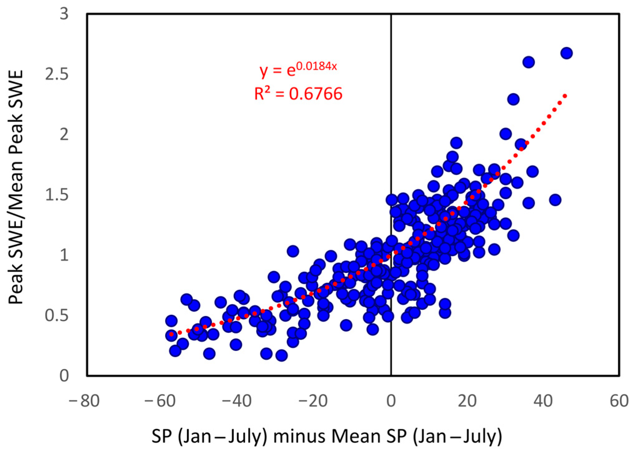
  69. Heldmyer, A.; Livneh, B.; Molotch, N.; Rajagopalan, B. Investigating the Relationship Between Peak Snow-Water Equivalent and Snow Timing Indices in the Western United States and Alaska. Water Resour. Res. 2021, 57, e2020WR029395. [Google Scholar] [CrossRef]
  70. Selkowitz, D.J.; Forster, R.R. Automated mapping of persistent ice and snow cover across the western US with Landsat. ISPRS J. Photogramm. Remote Sens. 2016, 117, 126–140. [Google Scholar] [CrossRef]
  71. U.S. Geological Survey (USGS) Earth Resources Observation and Science (EROS) Center. USGS EROS Archive-Landsat Collection 2 Level-3 Fractional Snow Covered Area (fSCA) Science Product; U.S. Geological Survey: Reston, VA, USA, 2022. [CrossRef]
  72. Dai, A. Temperature and pressure dependence of the rain-snow phase transition over land and ocean. Geophys. Res. Lett. 2008, 35, L12802. [Google Scholar] [CrossRef]
  73. Wayand, N.E.; Marsh, C.B.; Shea, J.M.; Pomeroy, J.W. Globally scalable alpine snow metrics. Remote Sens. Environ. 2018, 213, 61–72. [Google Scholar] [CrossRef]
  74. Hammond, J.C.; Saavedra, F.A.; Kampf, S.K. How Does Snow Persistence Relate to Annual Streamflow in Mountain Watersheds of the Western U.S. with Wet Maritime and Dry Continental Climates? Water Resour. Res. 2018, 54, 2605–2623. [Google Scholar] [CrossRef]
  75. Trujillo, E.; Molotch, N.P. Snowpack regimes of the Western United States. Water Resour. Res. 2014, 50, 5611–5623. [Google Scholar] [CrossRef]
  76. Sturm, M.; Wagner, A.M. Using repeated patterns in snow distribution modeling: An Arctic example. Water Resour. Res. 2010, 46, W12549. [Google Scholar] [CrossRef]
  77. Vögeli, C.; Lehning, M.; Wever, N.; Bavay, M. Scaling Precipitation Input to Spatially Distributed Hydrological Models by Measured Snow Distribution. Front. Earth Sci. 2016, 4, 108. [Google Scholar] [CrossRef]
  78. Pflug, J.M.; Lundquist, J.D. Inferring Distributed Snow Depth by Leveraging Snow Pattern Repeatability: Investigation Using 47 Lidar Observations in the Tuolumne Watershed, Sierra Nevada, California. Water Resour. Res. 2020, 56, e2020WR027243. [Google Scholar] [CrossRef]
  79. Deems, J.S.; Fassnacht, S.R.; Elder, K.J. Interannual Consistency in Fractal Snow Depth Patterns at Two Colorado Mountain Sites. J. Hydrometeorol. 2008, 9, 977–988. [Google Scholar] [CrossRef]
  80. McGrath, D.; Sass, L.; O’Neel, S.; McNeil, C.; Candela, S.G.; Baker, E.H.; Marshall, H.-P. Interannual snow accumulation variability on glaciers derived from repeat, spatially extensive ground-penetrating radar surveys. Cryosphere 2018, 12, 3617–3633. [Google Scholar] [CrossRef]
  81. Arsenault, K.R.; Houser, P.R.; De Lannoy, G.J.M.; Dirmeyer, P.A. Impacts of snow cover fraction data assimilation on modeled energy and moisture budgets. J. Geophys. Res. Atmos. 2013, 118, 7489–7504. [Google Scholar] [CrossRef]
  82. López-Moreno, J.I.; Gascoin, S.; Herrero, J.; Sproles, E.A.; Pons, M.; Alonso-González, E.; Hanich, L.; Boudhar, A.; Musselman, K.N.; Molotch, N.P.; et al. Different sensitivities of snowpacks to warming in Mediterranean climate mountain areas. Environ. Res. Lett. 2017, 12, 074006. [Google Scholar] [CrossRef]
  83. Marshall, A.M.; Abatzoglou, J.T.; Link, T.E.; Tennant, C.J. Projected Changes in Interannual Variability of Peak Snowpack Amount and Timing in the Western United States. Geophys. Res. Lett. 2019, 46, 8882–8892. [Google Scholar] [CrossRef]
  84. Musselman, K.N.; Lehner, F.; Ikeda, K.; Clark, M.P.; Prein, A.F.; Liu, C.; Barlage, M.; Rasmussen, R. Projected increases and shifts in rain-on-snow flood risk over western North America. Nat. Clim. Chang. 2018, 8, 808–812. [Google Scholar] [CrossRef]
  85. Liston, G.E. Representing Subgrid Snow Cover Heterogeneities in Regional and Global Models. J. Clim. 2004, 17, 1381–1397. [Google Scholar] [CrossRef]
  86. López-Moreno, J.I.; Fassnacht, S.R.; Heath, J.T.; Musselman, K.N.; Revuelto, J.; Latron, J.; Morán-Tejeda, E.; Jonas, T. Small scale spatial variability of snow density and depth over complex alpine terrain: Implications for estimating snow water equivalent. Adv. Water Resour. 2013, 55, 40–52. [Google Scholar] [CrossRef]
  87. Rittger, K.; Krock, M.; Kleiber, W.; Bair, E.H.; Brodzik, M.J.; Stephenson, T.R.; Rajagopalan, B.; Bormann, K.J.; Painter, T.H. Multi-sensor fusion using random forests for daily fractional snow cover at 30 m. Remote Sens. Environ. 2021, 264, 112608. [Google Scholar] [CrossRef]
  88. Gascoin, S.; Barrou Dumont, Z.; Deschamps-Berger, C.; Marti, F.; Salgues, G.; López-Moreno, J.I.; Revuelto, J.; Michon, T.; Schattan, P.; Hagolle, O. Estimating Fractional Snow Cover in Open Terrain from Sentinel-2 Using the Normalized Difference Snow Index. Remote Sens. 2020, 12, 2904. [Google Scholar] [CrossRef]
  89. Meyer, J.; Horel, J.; Kormos, P.; Hedrick, A.; Trujillo, E.; Skiles, S.M. Operational water forecast ability of the HRRR-iSnobal combination: An evaluation to adapt into production environments. Geosci. Model Dev. 2023, 16, 233–250. [Google Scholar] [CrossRef]
  90. Bair, E.H.; Rittger, K.; Davis, R.E.; Painter, T.H.; Dozier, J. Validating reconstruction of snow water equivalent in California’s Sierra Nevada using measurements from the NASA Airborne Snow Observatory. Water Resour. Res. 2016, 52, 8437–8460. [Google Scholar] [CrossRef]
  91. Dawson, N.; Broxton, P.; Zeng, X. Evaluation of Remotely Sensed Snow Water Equivalent and Snow Cover Extent over the Contiguous United States. J. Hydrometeorol. 2018, 19, 1777–1791. [Google Scholar] [CrossRef]
  92. Broxton, P.D.; Dawson, N.; Zeng, X. Linking snowfall and snow accumulation to generate spatial maps of SWE and snow depth. Earth Space Sci. 2016, 3, 246–256. [Google Scholar] [CrossRef]
  93. Lehning, M.; Völksch, I.; Gustafsson, D.; Nguyen, T.A.; Stähli, M.; Zappa, M. ALPINE3D: A detailed model of mountain surface processes and its application to snow hydrology. Hydrol. Process. 2006, 20, 2111–2128. [Google Scholar] [CrossRef]
  94. Pflug, J.M.; Hughes, M.; Lundquist, J.D. Downscaling Snow Deposition Using Historic Snow Depth Patterns: Diagnosing Limitations From Snowfall Biases, Winter Snow Losses, and Interannual Snow Pattern Repeatability. Water Resour. Res. 2021, 57, e2021WR029999. [Google Scholar] [CrossRef]
  95. Reynolds, D.S.; Pflug, J.M.; Lundquist, J.D. Evaluating Wind Fields for Use in Basin-Scale Distributed Snow Models. Water Resour. Res. 2021, 57, e2020WR028536. [Google Scholar] [CrossRef]
  96. Henn, B.; Newman, A.J.; Livneh, B.; Daly, C.; Lundquist, J.D. An assessment of differences in gridded precipitation datasets in complex terrain. J. Hydrol. 2018, 556, 1205–1219. [Google Scholar] [CrossRef]
  97. Raleigh, M.S.; Small, E.E. Snowpack density modeling is the primary source of uncertainty when mapping basin-wide SWE with lidar. Geophys. Res. Lett. 2017, 44, 3700–3709. [Google Scholar] [CrossRef]
  98. PlanetTeam. Planet Application Program Interface: In Space for Life on Earth. San Francisco, CA, 2024. Available online: https://api.planet.com/ (accessed on 3 January 2024).
Figure 1. Study area map showing the (1) snow modeling domain location within the north-central Colorado Rocky Mountains, US [43], (2) snow modeling calibration domain within the study area [43], (3) boundary of Rocky Mountain National Park (RMNP), (4) boundary of the East Troublesome Fire [44], (5) basin areas of interest within the study area, (6) SNOwpack TELemetry Network (SNOTEL) station locations [45], and (7) Airborne Snow Observatories (ASO) survey areas [46].
Remotesensing 17 01704 g001
Figure 2. Conceptual diagram of SnowModel inputs, submodels, and outputs, along with a flow chart of the workflows used in this study for calibration and real-time application and post-processing. Diagram modified from previous publication [59].
Remotesensing 17 01704 g002
Figure 3. Exponential relation developed between snow persistence (SP) and peak snow water equivalent (SWE) for all SNOTEL stations within the study domain. This relation was computed based on the site-specific normalized difference in SP (SP minus mean SP) and the site-specific normalized ratio of peak SWE to mean peak SWE [45].
Remotesensing 17 01704 g003
Figure 4. Time series plots and root mean squared error (RMSE) statistics for daily mean percent snow-covered area (SCA) across the model domain, comparing MODIS observations [64] with SCA simulated by the (a) default SnowModel version (SnowModeldefault), (b) calibrated SnowModel version (SnowModelcalibrated), and (c) SnowModel version calibrated with Landsat correction field (SnowModelLandsat) for water years 2016 through 2020 [43].
Remotesensing 17 01704 g004
Figure 5. Mean annual snow persistence (SP) and difference from Landsat-derived SP across the study area domain for water years 2000 through 2020, and the spatial efficiency metric (SPAEF) statistics (including correlation [α], ratio of coefficient of variation [β], and histogram match [γ]) [65] for the (a) default SnowModel version (SnowModeldefault), (b) calibrated SnowModel version (SnowModelcalibrated), and (c) SnowModel version calibrated with Landsat correction field (SnowModelLandsat) [43], as compared to the (d) Landsat observations [71]. Mean SP bias is shown in blue text. Bolded SPAEF statistics indicate the best value.
Remotesensing 17 01704 g005
Figure 6. Time series comparison plots of mean snow water equivalent (SWE) across the Big Thompson Basin for water years 2016 through 2020 simulated by the default SnowModel version without SNOTEL assimilation (SnowModeldefault_noassim), default SnowModel version (SnowModeldefault), calibrated SnowModel version (SnowModelcalibrated), SnowModel version calibrated with Landsat correction field (SnowModelLandsat), and the Snow Data Assimilation (SNODAS) model for (a) high elevations, (b) middle elevations, and (c) low elevations.
Remotesensing 17 01704 g006
Figure 7. Combination of violin plot and boxplot of simulated snow water equivalent (SWE) distribution, simulated mean SWE value, and root mean squared error (RMSE) for SNODAS, the default SnowModel version without SNOTEL assimilation (SnowModeldefault_noassim), default SnowModel version (SnowModeldefault), calibrated SnowModel version (SnowModelcalibrated), and SnowModel version calibrated with Landsat correction field (SnowModelLandsat) [43], as compared to Airborne Snow Observatories (ASO)-derived SWE for (a) 18 April 2022 and (b) 26 May 2022 across the Windy Gap Basin [46].
Remotesensing 17 01704 g007
Figure 8. Maps of simulated snow water equivalent (SWE) distribution and difference from Airborne Snow Observatories (ASO)-derived SWE for the(a) SNODAS, (b) default SnowModel version without SNOTEL assimilation (SnowModeldefault_noassim), (c) default SnowModel version (SnowModeldefault), (d) calibrated SnowModel version (SnowModelcalibrated), and (e) SnowModel version calibrated with Landsat correction field (SnowModelLandsat) [43], as compared to (f) Airborne Snow Observatories (ASO)-derived SWE for 26 May 2022 across the Windy Gap Basin [46].
Remotesensing 17 01704 g008
Figure 9. Map and elevation-based comparison of snow water equivalent (SWE) distribution between SnowModelLandsat, SnowModelSCA_update [43], and Airborne Snow Observatories (ASO) for the (a) Shadow Mountain Basin on 26 May 2022, (b) Shadow Mountain Basin on 27 May 2023, and (c) Big Thompson Basin on 21 May 2023 [46].
Remotesensing 17 01704 g009
Figure 10. Map of snow water equivalent (SWE) distribution difference between Airborne Snow Observatories (ASO)-derived SWE and SnowModelLandsat and SnowModelSCA_update [43] for the (a) Shadow Mountain Basin on 26 May 2022, (b) Shadow Mountain Basin on 27 May 2023, and (c) Big Thompson Basin on 21 May 2023 [46].
Remotesensing 17 01704 g010
Figure 11. Time series comparison (ac) and difference (bd) in mean snow water equivalent (SWE) for the Shadow Mountain Basin, for dates corresponding with Landsat SCA observations (January through August), between SnowModelLandsat and SnowModelSCA_update for (a,b) water years 2010 through 2012 and (c,d) water years 2018 through 2020 [43].
Remotesensing 17 01704 g011
Table 1. SnowModel configurations used in this study.
SnowModel Configuration NameSnowModel Configuration Description
SnowModeldefault_noassimDefault SnowModel parameters without data assimilation.
SnowModeldefaultDefault SnowModel parameters with data assimilation of SNOwpack TELemetry Network (SNOTEL) snow water equivalent (SWE).
SnowModelcalibratedCalibrated SnowModel parameters with data assimilation of SNOTEL SWE.
SnowModelLandsatCalibrated SnowModel parameters with data assimilation of SNOTEL SWE and Landsat snow persistence (SP) precipitation correction field.
SnowModelSCA_updateSnowModelLandsat gridded outputs post-processed and updated for dates corresponding with remotely sensed snow-covered area (SCA) images.
Table 3. Selected performance statistics [Root Mean Squared Error (RMSE) and Nash–Sutcliffe Efficiency (NSE)] based on grid-by-grid SNODAS and SnowModelLandsat [SnowModel version calibrated with Landsat correction field] simulated snow water equivalent (SWE) compared to Airborne Snow Observatories (ASO)-derived SWE for 18 April 2022 and 26 May 2022 across the Windy Gap Basin. Performance statistics are provided for all elevations: high elevations (>3124 m), middle elevations (2438–3124 m), and low elevations (<2438 m). “---” indicates zero snow observed. Additional performance statistics are provided in Table S3.
18 April 202226 May 2022
Model VersionSNODASSnowModelLandsatSNODASSnowModelLandsat
All ElevationsModel mean SWE (mm)27219613898
ASO mean SWE (mm)223223104104
RMSE (mm)193137199121
NSE0.130.560.000.63
High ElevationsModel mean SWE (mm)405320309273
ASO mean SWE (mm)406406284284
RMSE (mm)260200307203
NSE−0.380.18−0.420.38
Middle ElevationsModel mean SWE (mm)2091365411
ASO mean SWE (mm)1351351414
RMSE (mm)1509111438
NSE−0.560.44−4.650.38
Low ElevationsModel mean SWE (mm)18100
ASO mean SWE (mm)101000
RMSE (mm)2023------
NSE−0.07−0.36------
Disclaimer/Publisher’s Note: The statements, opinions and data contained in all publications are solely those of the individual author(s) and contributor(s) and not of MDPI and/or the editor(s). MDPI and/or the editor(s) disclaim responsibility for any injury to people or property resulting from any ideas, methods, instructions or products referred to in the content.

