Article

Precipitation Retrieval from Geostationary Satellite Data Based on a New QPE Algorithm

1
Asia-Pacific Typhoon Collaborative Research Center, Shanghai 201306, China
2
Shanghai Typhoon Institute of China Meteorological Administration, Shanghai 200030, China
*
Author to whom correspondence should be addressed.
Remote Sens. 2025, 17(10), 1703; https://doi.org/10.3390/rs17101703
Submission received: 8 April 2025 / Revised: 6 May 2025 / Accepted: 10 May 2025 / Published: 13 May 2025

Abstract

:
A new quantitative precipitation estimation (QPE) method for Himawari-9 (H9) and Fengyun-4B (FY4B) satellites has been developed based on cloud top brightness temperature (TBB). The 24-hour, 6-hour, and hourly rainfall estimates of H9 and FY4B have been compared with rain gauge datasets and precipitation estimation data from the GPM IMERG V07 (IMERG) and Global Precipitation Satellite (GSMaP) products, especially based on the case study of landfalling super typhoon “Doksuri” in 2023. The results indicate that the bias-corrected QPE algorithm substantially improves precipitation estimation accuracy across multiple temporal scales and intensity categories. For extreme precipitation events (≥100 mm/day), the FY4B-based estimates exhibit markedly better performance. Furthermore, in light-to-moderate rainfall (0.1–24.9 mm/day) and heavy rain to rainstorm ranges (25.0–99.9 mm/day), its retrievals are largely comparable to those from IMERG and GSMaP, demonstrating robust consistency across varying precipitation intensities. Therefore, the new QPE retrieval algorithm in this study could largely improve the accuracy and reliability of satellite precipitation estimation for extreme weather events such as typhoons.

1. Introduction

Precipitation is a crucial component of Earth’s energy cycle and material exchange, serving as a vital driver of terrestrial ecosystems and playing a decisive role in climate change [1,2]. Long-term precipitation records are essential for quantifying the global water cycle, supporting and validating numerical models, and providing climate context data for various water resource management activities [3,4]. Traditional precipitation monitoring methods primarily rely on ground-based observing stations. However, the distribution of these stations is often very uneven, with limited regional coverage. This is especially true in complex mountainous areas and most oceans, where the station distribution is sparse, leading to significant data gaps making it difficult to achieve large-scale spatial continuity in monitoring [5,6]. To address this limitation, satellite remote sensing technology has emerged as an important complementary method for precipitation monitoring. Geostationary meteorological satellites have consistent detection capabilities and thus can provide continuous all-weather and high-frequency observations of the same region, offering wide coverage and high temporal resolution. This capability helps fulfill the demand for precipitation data in areas with sparse meteorological stations and regions lacking weather radar coverage [7,8]. Typhoons are intense tropical cyclones characterized by strong winds, heavy rainfall, and organized convective systems. Their precipitation structure is highly dynamic, with deep convective cores and spiral rainbands contributing to extreme rainfall, often bringing intense and prolonged rainfall that leads to severe flooding, landslides, and infrastructure damage. Accurate and timely estimation of typhoon precipitation is crucial for disaster preparedness, early warning systems, and hydrological modeling, helping to mitigate economic losses and protect human lives.
Satellite-based quantitative precipitation estimation (QPE) is crucial in monitoring and predicting precipitation, particularly for extreme weather events such as typhoons [9]. Accurately estimating typhoon precipitation is essential for disaster prevention, hydrological forecasting, and climate studies [10,11]. However, estimating precipitation from landfalling typhoons remains challenging due to the complex and dynamic nature of typhoon systems, which involve intense convective precipitation, rapid cloud evolution, and strong interactions with topography.
Traditional QPE methods based on visible and infrared remote sensing infer precipitation by analyzing cloud properties. For example, the precipitation estimation from remotely sensed information using artificial neural networks (PERSIANN) algorithm utilizes infrared (IR) brightness temperature from geostationary satellites combined with ground-based data to estimate precipitation using an adaptive artificial neural network approach [12]. Building on this, the PERSIANN-Cloud Classification System (PERSIANN-CCS) further classifies clouds into different clusters based on thresholding techniques, establishing characteristic curves for each cluster (cloud top temperature and rainfall) [13]. The PERSIANN-CCS method has been integrated into the widely used Global Precipitation Measurement (IMERG) product. Braithwaite et al., combined PERSIANN with ground observations to create a long-term climate precipitation dataset called PERSIANN-CDR (PERSIANN-Climate Data Record) [3].
Several studies have attempted to improve typhoon precipitation estimation using satellite data. Yue et al., employed cloud motion extrapolation to forecast short-term convective rainfall intensity in tropical cyclone conditions [14]. Zhang et al. conducted correlation analyses between the infrared brightness temperature from GMS-5 and precipitation forecasts to establish a short-term QPE model [9]. More recently, Ma et al. introduced an all-weather near-real-time QPE framework based on multi-spectral analysis (MSA), leveraging data from the Advanced Geostationary Radiation Imager (AGRI) aboard the FengYun-4 series satellites to enhance precipitation retrievals [15].
Despite these advances, existing methods still face significant challenges in estimating the extreme precipitation associated with typhoons. Many traditional methods have difficulty capturing strong convective precipitation, especially due to the limitations of infrared technology in detecting deep convective clouds and precipitation structures under strong cloud cover. This difficulty results in significant errors in the current methods for heavy precipitation, with the estimated precipitation being mostly lower than the true value. Machine learning and deep learning methods have shown promise in improving precipitation estimation by learning the complex relationship between satellite observations and precipitation. For example, Min et al. combined the infrared brightness temperature of Himawari-8 with numerical weather forecasting to develop a precipitation estimation model based on random forests [16]. Sehad et al., applied support vector machines to the northern region of Algeria to achieve precipitation estimation [17]. Similarly, Wang et al. used a convolutional neural network (CNN) trained in mainland United States and adjusted it using Fengyun satellite data to improve precipitation estimation in China [18]. A key prerequisite for using machine learning and deep learning is having a good training dataset. However, due to the relatively low amount of extreme precipitation events such as typhoons, it is difficult to obtain a large amount of heavy-precipitation datasets. Therefore, existing precipitation algorithms and related products still have significant limitations in estimating heavy-rainfall events such as typhoons.
Currently, common rainfall products include those derived from satellite missions such as the Tropical Rainfall Measuring Mission (TRMM) and the Global Precipitation Measurement (GPM) mission, as well as the Climate Prediction Center’s MORPHing technique (CMORPH). These products are based on data from both microwave and infrared sensors on the respective satellites. Numerous studies have assessed the performance of these products. For example, Wang et al., evaluated the performance of GPM IMERG and TRMM 3B42V7 in the arid region of Northwest China, finding that IMERG performed well in detecting precipitation events but had a high false alarm rate, particularly in overestimating light precipitation [19]. In another study, Wang et al. compared IMERG and TRMM, revealing that IMERG showed improvement in overestimating light precipitation and had better capability in reproducing precipitation intensity compared to TRMM Multi-satellite Precipitation Analysis (TMPA) [20]. Zhang et al., assessed the performance of GPM, TRMM, and CMORPH in the Tianshan Mountains, finding that GPM performed best at lower to middle rainfall amounts (5–25 mm/day) but still exhibited underestimation issues in light rainfall (<5 mm/day) [21]. However, most of these studies have focused on evaluating daily precipitation, with fewer studies on extreme precipitation events such as typhoons. Although Yu et al., compared the accuracy of TRMM 3B42, CMORPH, and GMS5-TBB in typhoon precipitation, they did not involve the Himawari and FengYun series satellites [22]. With the rapid development of the Himawari (H9) and FengYun (FY4B) series satellites, their high temporal and spatial resolution and multi-channel observation data provide significant value in precipitation monitoring and weather forecasting [16].
Therefore, this study developed a new QPE algorithm based on Adler [23], Goldenberg [24], and Yue [14] to improve the accuracy and reliability of geostationary satellites in typhoon heavy-precipitation inversion. We adjusted the formula for convective precipitation rate based on hourly rainfall data from automatic ground stations during typhoon landfall events and compared the inverted precipitation results with measured precipitation values (2017–2022) using the least squares method to construct a regression correction equation to improve the accuracy of inverted heavy precipitation. It will apply the algorithm to high-resolution geostationary satellite data (H9 and FY4B) for the inversion of heavy rainfall caused by landfalling typhoons and evaluate in detail the accuracy of the inversion results under different time scales and precipitation intensities. The ultimate goal is to develop high-precision precipitation products to meet the needs of climate change and disaster management, particularly in monitoring typhoon-related heavy-precipitation events, thereby providing a solid data foundation to reduce the impact of severe precipitation and associated secondary disasters.

2. Materials and Methods

2.1. Data

This study uses Himawari-9 (H9) and Fengyun-4B (FY4B) satellite data to develop a QPE method based on cloud top brightness temperature (TBB). The rainfall estimates of H9 and FY4B are compared with the precipitation estimate datasets from the GPM IMERG V07 (IMERG) and Global Precipitation Satellite (GSMaP) products based on the case study of landfalling super typhoon “Doksuri” in 2023. Rain gauge datasets are also used in this study as a rain observation truth for reference.

2.1.1. H9 Data

H9 is a next-generation geostationary meteorological satellite launched by the Japan Aerospace Exploration Agency’s Earth Observation Research Center. It can capture full-disk observations in just 10 min and features multiple spectral channels with high temporal and spatial resolution, which is advantageous for monitoring the development and changes of heavy-rainfall cloud systems. It is equipped with the Advanced Himawari Imager (AHI), which has 16 channels [25]. This study uses Level 1 data from the Himawari-9 satellite’s AHI, specifically with a central wavelength of 11.2 μm, which has undergone radiometric calibration and geographic positioning preprocessing. The data has a spatial resolution of 2 km, a temporal resolution of 10 min, and covers the range of 60°N to 60°S and 80°E to 160°W. The data are sourced from the website http://www.eorc.jaxa.jp/ptree/index.html (accessed on 22 April 2024).

2.1.2. FY4B Data

FY4B is the first operational meteorological satellite in China’s second-generation geostationary meteorological satellite series. It works alongside FengYun-4A, FengYun-2H, FengYun-2G, and FengYun-2F to form China’s geostationary meteorological satellite observation network, gradually replacing Fengyun-2 and becoming a key component of the World Meteorological Organization’s global satellite observation system. FengYun-4B carries four main payloads: the Advanced Geostationary Radiation Imager (AGRI), the Geostationary Interferometric Infrared Sounder (GIIRS), the Rapid Imaging Instrument (GHI), and the Space Environment Monitoring Package (SEP). AGRI features 15 channels and adds a low-level water vapor channel (7.24–7.6 μm) compared to FengYun-4A, allowing it to capture rapid changes in low-level water vapor. The spatial resolution for visible and near-infrared channels is 0.5–1 km, while the infrared channels have a 2–4 km resolution. AGRI’s observation mode is consistent with that of FengYun-4A, capturing full-disk images every 15 min, along with a variable regional observation mode [15]. This study utilizes brightness temperature data from the infrared channel, with a central wavelength of 10.8 μm, in AGRI. The data feature a temporal resolution of 15 min and a spatial resolution of 4 km, covering the range from 60°N to 60°S and 80°E to 160°W. The data are sourced from the website http://satellite.nsmc.org.cn/PortalSite/Data/Satellite.aspx (accessed on 10 April 2024).

2.1.3. IMERG Precipitation Data

The Global Precipitation Measurement (GPM) IMERG is a global precipitation dataset (https://pmm.nasa.gov/ (accessed on 7 July 2024)). The IMERG product integrates various data sources, including satellite-derived microwave precipitation estimates, microwave-calibrated infrared estimates, ground gauge measurements, and other potential datasets, at spatial and temporal resolutions of 0.1° × 0.1° and half-hourly intervals [26]. The IMERG V07 is intended to intercalibrate, merge, and interpolate all satellite microwave precipitation estimates, together with microwave-calibrated infrared (IR) satellite estimates, precipitation gauge analyses, and potentially other precipitation estimators at fine time and space scales for the TRMM and GPM eras over the entire globe [27]. This study selects the hourly-scale precipitation product IMERG V07 with a resolution of 0.1° × 0.1° as the data source for cross-validation in this research.

2.1.4. GSMaP Precipitation Data

The GSMaP dataset, developed by the Japan Aerospace Exploration Agency (JAXA), aims to provide high spatiotemporal resolution global precipitation estimates by integrating observations from multiple meteorological satellites (https://sharaku.eorc.jaxa.jp/GSMaP/ (accessed on 10 July 2024)). This dataset primarily relies on microwave and infrared observations and uses a combination of physical models and machine learning algorithms to deliver accurate precipitation estimates. GSMaP has a temporal resolution of hourly intervals and a spatial resolution of 0.1° × 0.1°, covering the globe [28]. Compared to other precipitation data sources such as IMERG and CMORPH, GSMaP has its own advantages in different regions and sometimes performs better in capturing short-duration intense precipitation events in tropical areas [29]. In this study, the GSMaP_Gauge (hereafter referred to as GSMaP) dataset is used as a reference data source with the same spatial resolution as the IMERG dataset, 0.1° × 0.1°.

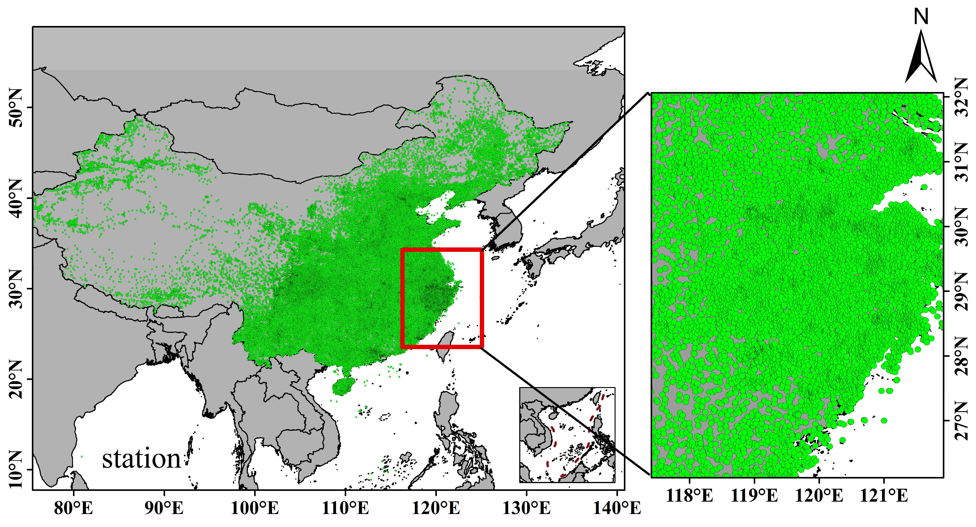
2.1.5. Gauge Rain Data

Ground station rain gauges have the advantages of high accuracy, strong real-time performance, and good adaptability. They can directly measure precipitation, provide accurate local precipitation data, deploy flexibly, and are suitable for long-term monitoring. This study used a large number of measured precipitation values (2017–2022) and applied the least squares method to correct the gridded precipitation rate values, resulting in higher-precision precipitation rates, and constructed a regression correction equation. The ground observation station data also serve as a reference truth for comparing the satellite estimate results of the new QPE algorithm in this study. It uses hourly precipitation data from ground meteorological stations in China from 1 July to 31 July 2023, providing detailed observational information on the precipitation during the landfall of typhoon “Doksuri”. Figure 1 shows the spatial distribution of the ground meteorological stations, which are densely distributed in the southeastern coastal region of China.

2.2. Methods

2.2.1. QPE Method

Based on the previous work of Adler and Negri (AN) [23], Goldenberg [24], and Li [30], a preliminary method of QPE for landfalling typhoons was proposed by Yue [14] using GMS5 infrared channel 1 (IR1) TBB data. Through parameter modification and adjustment, a new precipitation estimation method suitable for landfalling typhoons using H9 and FY4B satellite data has been developed in this study. The calculation process is as follows:
(1) Determining the Convective Core: Calculate the minimum temperature ( T m i n ) convective slope parameter  S i , j  (Equation (1)) and the critical value of the convective slope (Equation (2)). For grid points with a TBB not exceeding 253 K, evaluate whether the TBB of the point is less than or equal to the surrounding 4 (top, bottom, left, right) adjacent grid points. If so, the corresponding cloud top temperature is denoted as  T m i n .
S i , j = 4 [ T i 1 , j + T i + 1 , j 2 T i , j E W + T i , j 1 + T i , j + 1 2 T i , j N S ]
S l o p e = e x p [ 0.0826 ( T m i n 217 ) ]
Equations (1) and (2) here are improved and applicable to FY4B and H9. The original formulas were designed by Adler, Negri, and Goldenberg to calculate the GOES satellite, and they constructed relationships based on radar data. In the equations, T represents TBB, △EW = △NS denotes the satellite’s horizontal resolution (2 km for H9 and 4 km for FY4B), and Δ = 5.6 km is the horizontal resolution for the GOES satellite [23]. If  S i , j  >= the slope, the grid point corresponding to  T m i n  is determined to be the convective core. Due to the differences in FY4B, H9, and GOES satellites, we have increased the minimum cloud top temperature for landing typhoons from 207 in Equation (2) to 217. Here, the convective core is the area with the strongest updraft in the precipitation system, dominating the production of heavy precipitation and affecting the accuracy of precipitation inversion. The convective tilt parameter is used to determine whether there is precipitation in the convective region.
(2) Establishing the Correction Formula: Due to the difference in horizontal resolution between the visible satellite field and the one-dimensional cloud model, it is not feasible to directly calculate the convective precipitation coverage area and average convective precipitation rate. Therefore, it is necessary to derive the correction value  T C  for  T m i n  separately for H9 (Equation (4)) and FY4B (Equation (5)) based on the differences in horizontal resolution between H9, FY4B, and the GOES satellite (Equation (3)).
T m i n T C = 0.283 × T m i n 56.6 ,     T m i n > 200 K 0                                                                 ,     T m i n 200 K
T m i n T C = 0.046 × T m i n 9.13 , T m i n > 200 K 0                                                                 , T m i n 200 K
T m i n T C = 0.183 × T m i n 36.52 ,       T m i n > 200 K 0                                                                 ,       T m i n 200 K
Here, because the resolutions of FY4B, H9, and GOES are different, we use the Goldenberg method to correct the different satellite data [24]. That is, we divide the GOES satellite horizontal resolution area of 8.0 × 3.1 (=24.8 km2) by the FY4B and H9 horizontal resolution area of 4 × 4 (=16 km2), 2 × 2 (=4 km2), to obtain the correction factors 1.55 and 6.2. Then, we divide the right-hand side of Equation (3) by 1.55 and 6.2 to obtain Equations (4) and (5). For H9, temperature correction is performed if the convective core condition is met. For FY4B, a correction threshold is first established, which is the mean temperature  T m e a n  of all TBB values corresponding to the identified convective cores. If  T m i n  <  T m e a n   , temperature correction is then applied.
(3) Calculating Convective Precipitation Coverage Area  A r  (Equation (6)) and Average Convective Precipitation Rate ( R m e a n ) (Equation (8)): Calculate the convective precipitation coverage area  A r  (Equation (6)) and the average convective precipitation rate ( R m e a n ) (Equation (8)): The formula for the convective precipitation coverage area is obtained by simulating the observation profiles of Florida (summer) and Oklahoma (spring) through a series of cloud models calculated by AN and Goldenberg. The calculation of the convective precipitation coverage area in this study follows the methodologies of AN, Goldenberg, and Yue [14,23,24]. However, we have newly corrected the use of the formula. The original formula for precipitation coverage area assumes that there is a convective core M with a corresponding convective rain coverage radius of rm and an average convective precipitation rate of rm. For any grid point D on the cloud map, its distance from the convective core M is rd. If RD > RM, the D grid point will not be assigned RM. Conversely, if RD ≤ RM, the D grid point will be assigned Rm. If there is another convective core N at the same time, with a corresponding convective rain coverage radius of RN and an average convective precipitation rate of Rn, then grid point D will also be covered by the convective rain area generated by convective core N, i.e., RD ≤ RN, and this grid point D will also be assigned RN. In response to this situation, the processing method for AN and Goldenberg is to take the arithmetic mean. That is to say, for grid point D, the arithmetic mean of the different average convective precipitation rates assigned to it at the same time is taken, and this arithmetic mean is the final average convective precipitation rate of grid point D. This processing method makes the convective precipitation rate of grid point D easily change with the number of convective coverage areas. We believe that this processing method is difficult to accurately estimate the actual convective precipitation rate that may occur at point D. So, we proposed a new processing method, which means that for the grid points within the coverage area of convective rainfall, it is not simply assigning the same average convective precipitation rate to all but treating them separately. Because for each grid point within the coverage area, there is its own cloud top temperature TBB, which is corrected using Equations (4) and (5) to obtain its respective cloud top correction temperature. Then, the cloud top correction temperature is substituted into Equation (6) to calculate the convective precipitation rate of each grid point. This avoids the need for a simple arithmetic mean to determine the convective precipitation rate of a grid point when it is in multiple convective coverage areas. With the new calculation method, regardless of how many convective coverage areas a grid point is in at the same time, its corresponding convective precipitation rate is always unique and unchanged.
Similarly, the formula for calculating the convective precipitation rate has been adjusted based on hourly rainfall data from automated ground stations during typhoon landfall events. Latitude affects satellite precipitation retrieval, mainly reflected in atmospheric thickness, cloud characteristics, and seasonal variations. Equatorial regions have more precipitation and thicker clouds, while high-latitude regions have less precipitation and thinner clouds. In addition, satellite inversion needs to consider latitude differences to improve the accuracy of inversion. In this study, latitude was introduced as a variable in the original calculation formula. The average brightness temperature  T i  corresponding to the convective core that satisfies condition (1) is calculated using Equation (7). This  T s  is used as a threshold to compute the formula for estimating landfall typhoon precipitation intensity for H9 and FY4B satellites (Equation (8)). For each grid point under the convective precipitation coverage area, the cloud top temperature is corrected using step (2), and then the convective precipitation rate corresponding to that point is calculated based on the corrected temperature.
A r = e x p ( 15.27 0.0465 T C )
T s = 1 n i = 1 n T i
R m e a n = exp ( 0.0257 T C + 7.968 + cos ( 90 lat ) )   , T < T s exp ( 0.0257 T C + 7.468 )   , T T s
(4) Calculating Stratiform Precipitation: When the cloud top temperature of certain grid points is below the critical temperature and has not been assigned a convective precipitation rate, these grid points are classified as stratiform precipitation, with a 2 mm/h precipitation rate. For H9, the critical temperature is determined by first identifying the convective slope parameters corresponding to the  T m i n  grid points. If the convective slope parameter is less than 4, it is retained. The mean TBB of all retained convective slope parameters is then calculated, which serves as the critical temperature for H9. For FY4B, the critical temperature is identified similarly to the convective slope parameters which correspond to the  T m i n  grid points, and it is retained if the parameter is less than 4. The mean TBB of these retained parameters is computed, followed by calculating the mean of this value compared to  T m e a n  from step (2), which establishes the critical temperature for FY4B.

2.2.2. Correction Method

To better reduce the error in the retrieved precipitation results, this study constructed a regression correction equation by comparing inversion precipitation results with station-measured precipitation values (2017–2022) using the least squares method. This regression correction equation can further improve the precision and accuracy of the inversion results. The process is as follows:
First, a threshold is determined to divide the correction equation intervals, which is the mean TBB corresponding to the convective core. By analyzing the relationship between inversion precipitation and station-measured precipitation, it was found that different precipitation intensity intervals have varying levels of adaptability to the correction equation. Therefore, different correction equations need to be constructed for different precipitation intensities.
Next, based on the threshold, correction equations for two precipitation intensity intervals are constructed separately. The first interval applies to lighter or moderate precipitation, while the second interval applies to intense precipitation. These correction equations account for the nonlinear relationship between inversion precipitation and station-measured precipitation, providing targeted corrections for different levels of precipitation intensity.
Finally, the inversion precipitation results from the H9 and FY4B satellites are corrected using the constructed correction equations. By applying different correction equations, the biases caused by satellite inversion algorithms at different precipitation intensities can be effectively reduced, thus improving the reliability and accuracy of the precipitation inversion results.
Equations (9) and (10), corresponding to the H9 and FY4B satellites, respectively, show the specific correction equations. In these equations, the inversion precipitation values are adjusted based on the regression relationship with station-measured values. The corrected results better reflect the actual precipitation conditions, providing more accurate data support for subsequent meteorological analysis and typhoon research.
R H 9 , c o r r e c t = R H 9 , m e a n × 1.32 7.66 ,     T H 9 < T s R H 9 , m e a n × 0.53 + 1.55 ,     T H 9 T s
R F Y 4 B , c o r r e c t = R F Y 4 B , m e a n × 1.44 8.33 ,     T F Y 4 B < T s R F Y 4 B , m e a n × 0.62 + 1.74 ,     T F Y 4 B T s

2.2.3. Verification Method

To comprehensively evaluate the accuracy and reliability of the new QPE method in this study, we use gauge rain data as a reference to verify the different satellite QPE data results.
Firstly, we use bilinear interpolation to interpolate the different QPE results to the corresponding gauge stations and then compare them one by one. In addition, this study employs various statistical metrics for a thorough analysis, which include threat score (TS), equitable threat score (ETS), Heidke skill score (HSS), correlation coefficient (CC), probability of detection (POD), false alarm ratio (FAR), bias, and root mean square error (RMSE) [22]. These metrics allow for a systematic evaluation of the differences and consistency between satellite-retrieved precipitation data and rain gauge truth measurements. The relevant formulas can be found in Appendix A.

3. Results

3.1. Evaluation of Precipitation Results Across All Gauge Stations

The 24-hour, 6-hour, and hourly rainfall estimates of H9 and FY4B produced by this study have been compared with rain gauge datasets and also the precipitation estimation data from IMERG and GSMaP. We used the meteorological station data from the Chinese region in July 2023 to validate the inversion results of the algorithm. By comparing the inversion results with the actual observed data, we assessed the accuracy and reliability of the algorithm. This helped us identify the strengths and weaknesses of the algorithm and provided a basis for further optimization.

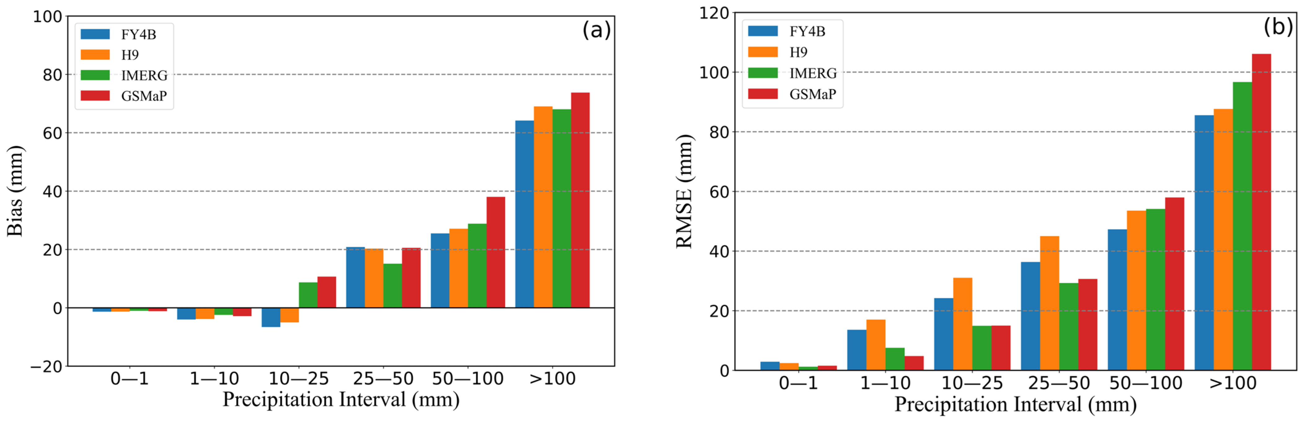
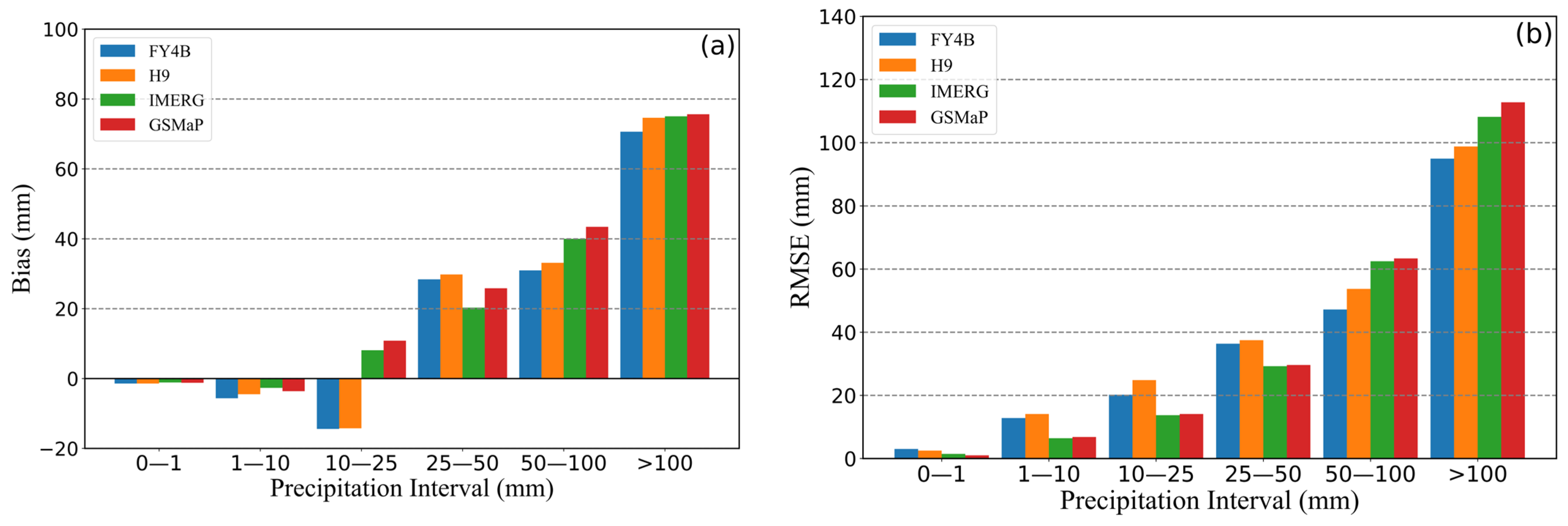
3.1.1. Results for 24-Hour Precipitation

Table 1 presents the validation results for 24-hour precipitation estimates from FY4B, H9, IMERG, and GSMaP under various precipitation thresholds. IMERG and GSMaP generally exhibit superior performance across key indicators such as TS, ETS, CC, and HSS for rainstorms and below (<100 mm). For instance, at a threshold of 1, both IMERG and GSMaP achieve a TS value of 0.54 and 0.52, an ETS value of 0.48 and 0.42, a CC value of 0.71 and 0.72, respectively, and an HSS value of 0.59. These results are significantly higher than those of FY4B (TS = 0.42, ETS = 0.38, CC = 0.66, HSS = 0.44) and H9 (TS = 0.45, ETS = 0.34, CC = 0.67, HSS = 0.51), indicating their stronger predictive ability for light rain events. Furthermore, the FAR values for IMERG and GSMaP are notably lower at lower thresholds. For example, at a threshold of 1, GSMaP’s FAR value is only 0.22, substantially lower than FY4B’s 0.36 and H9’s 0.26, further demonstrating the reliability of their predictions. In contrast, for rainstorms and above (≥100 mm), FY4B and H9 outperform IMERG and GSMaP, particularly in terms of POD and FAR. At a threshold of 250, FY4B’s POD value is 0.19, significantly higher than the 0.14 of IMERG and GSMaP, and its FAR value is 0.62, lower than IMERG’s 0.71 and GSMaP’s 0.66. Additionally, FY4B and H9 show strong performance in TS and ETS under the extreme heavy-rainstorm threshold. At a threshold of 250, FY4B’s TS value is 0.15, and its ETS value is 0.15, superior to IMERG’s TS (0.13) and ETS (0.11). H9 also performs better than IMERG, with a TS value of 0.11 and an ETS value of 0.11. Moreover, FY4B stands out with a high HSS value under the extreme heavy-rainstorm threshold. At a threshold of 250, FY4B’s HSS value is 0.28, significantly higher than IMERG’s 0.18 and GSMaP’s 0.17.
Figure 2 illustrates the 24-hour precipitation errors for FY4B, H9, IMERG, and GSMaP. Overall, IMERG performs best in the low-precipitation ranges (0–1 mm and 1–10 mm), exhibiting the smallest bias (−1.41 and −4.31), indicating minimal overestimation. Additionally, IMERG has the lowest RMSE (0.51 and 4.79), reflecting the highest prediction accuracy and making it well-suited for precipitation inversion in low-precipitation areas. However, as precipitation increases, IMERG’s performance declines, particularly in the high-precipitation range (>250 mm), where the bias increases significantly (110.88), indicating underestimation, and the RMSE peaks at 139.8, resulting in a sharp decrease in prediction accuracy. GSMaP demonstrates relatively balanced performance in the low-to-moderate-precipitation ranges, with bias and RMSE at moderate levels, especially closely matching IMERG in the low-precipitation range. Nevertheless, its bias (112.98) and RMSE (137.13) remain high in the high-precipitation range, indicating limited applicability in high-precipitation areas. In contrast, FY4B and H9 excel in the extreme heavy-rainstorm range (>250 mm), though some underestimation persists. Their biases (FY4B: 103.67; H9: 104.7) and RMSE (FY4B: 129.92; H9: 133) are relatively low, indicating high prediction accuracy and making them suitable for precipitation inversion in high-precipitation areas. However, in the rainstorm and below (<100 mm) ranges, both FY4B and H9 perform worse than IMERG and GSMaP, exhibiting large deviations and overestimation with high RMSE values, signaling limited effectiveness in these ranges.

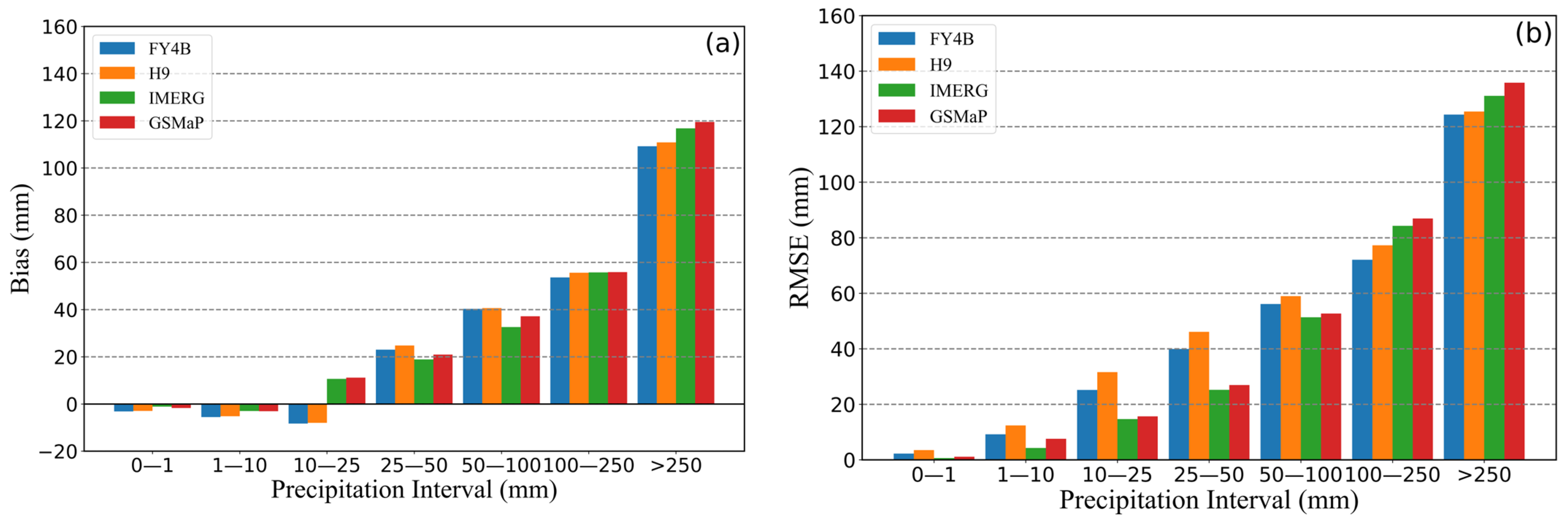
3.1.2. Results for 6-Hour Precipitation

Compared to the 24-hour results, the precipitation prediction performance at the 6-hour timescale shows a similar trend but with some differences in specific indicators (see Table 2). For instance, the TS, ETS, and CC values of IMERG and GSMaP in rainstorms <50mm are slightly lower on the 6-hour scale than on the 24-hour scale.
For rainstorms <50 mm, IMERG and GSMaP continue to perform the best in metrics like TS, ETS, CC, and HSS. For example, when the threshold is 1 mm, the TS values for IMERG and GSMaP are 0.48, the ETS values are 0.39, the CC values are 0.51 and 0.48, and the HSS values are 0.56, respectively. These values are significantly higher than those of FY4B and H9, indicating stronger predictive abilities for low-intensity precipitation events. Additionally, the FAR values for IMERG and GSMaP are lower at low thresholds. For instance, at a threshold of 1 mm, IMERG’s FAR is 0.30, and GSMaP’s FAR is 0.33, both significantly lower than FY4B’s 0.43 and H9’s 0.42, further confirming the reliability of their predictions. In rainstorms or above (≥50 mm), FY4B and H9 perform better, especially in POD and FAR. For example, at a threshold of 100 mm, FY4B’s POD is 0.16, significantly higher than the 0.11 of IMERG and GSMaP, and its FAR is 0.71, lower than IMERG’s 0.76 and GSMaP’s 0.79. At the same time, the TS, ETS, and HSS values for FY4B and H9 also show strong performance under the heavy-rainfall threshold. For example, at a threshold of 100 mm, FY4B’s TS is 0.14, ETS is 0.14, and HSS is 0.16, all higher than those of IMERG and GSMaP.
Compared to the 24-hour precipitation results, the error values for FY4B, H9, IMERG, and GSMaP in the 6-hour precipitation analysis have increased (see Figure 3). Analyzing the bias and root mean square error (RMSE), all four products (FY4B, H9, IMERG, GSMaP) tend to overestimate precipitation in the low range (“0–1”, “1–10”). FY4B and H9 also show overestimation in the “10–25” category. In the higher precipitation ranges (“25–50”, “50–100”, “>100”), all products exhibit underestimation, with the most significant bias observed in extreme rainfall (>100 mm). Among them, GSMaP shows the largest underestimation, with a value of 73.77. From the error perspective, the RMSE for all products increases as precipitation increases. IMERG has the smallest error (1.22) in the low-precipitation range but the largest error (96.67) in extreme precipitation (>100 mm). The underestimation of FY4B and H9 in extreme heavy rainstorms (>100 mm) is relatively smaller than that of IMERG and GSMaP, with FY4B at 64.19 and H9 at 69.04. Additionally, the RMSE of FY4B and H9 is lower than that of IMERG and GSMaP under extreme heavy rainstorms (>100 mm), with FY4B at 85.54 and H9 at 87.65. This further demonstrates the superior error control of FY4B and H9 in extreme heavy-rainstorm conditions.

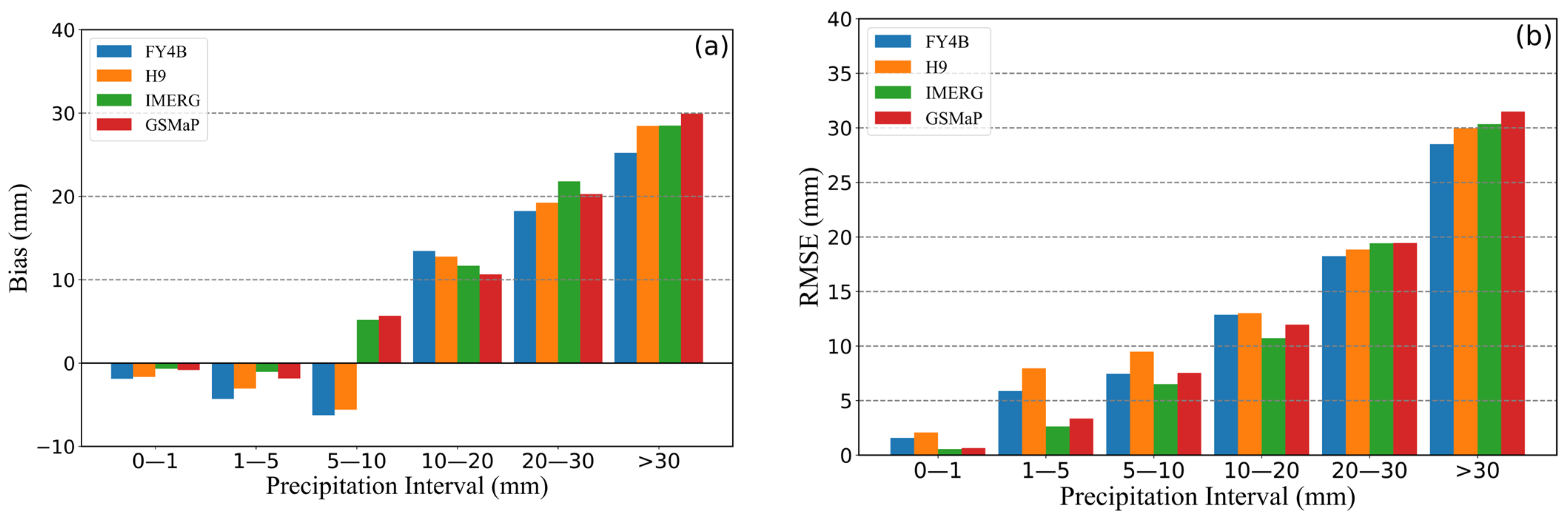
3.1.3. Results for Hourly Precipitation
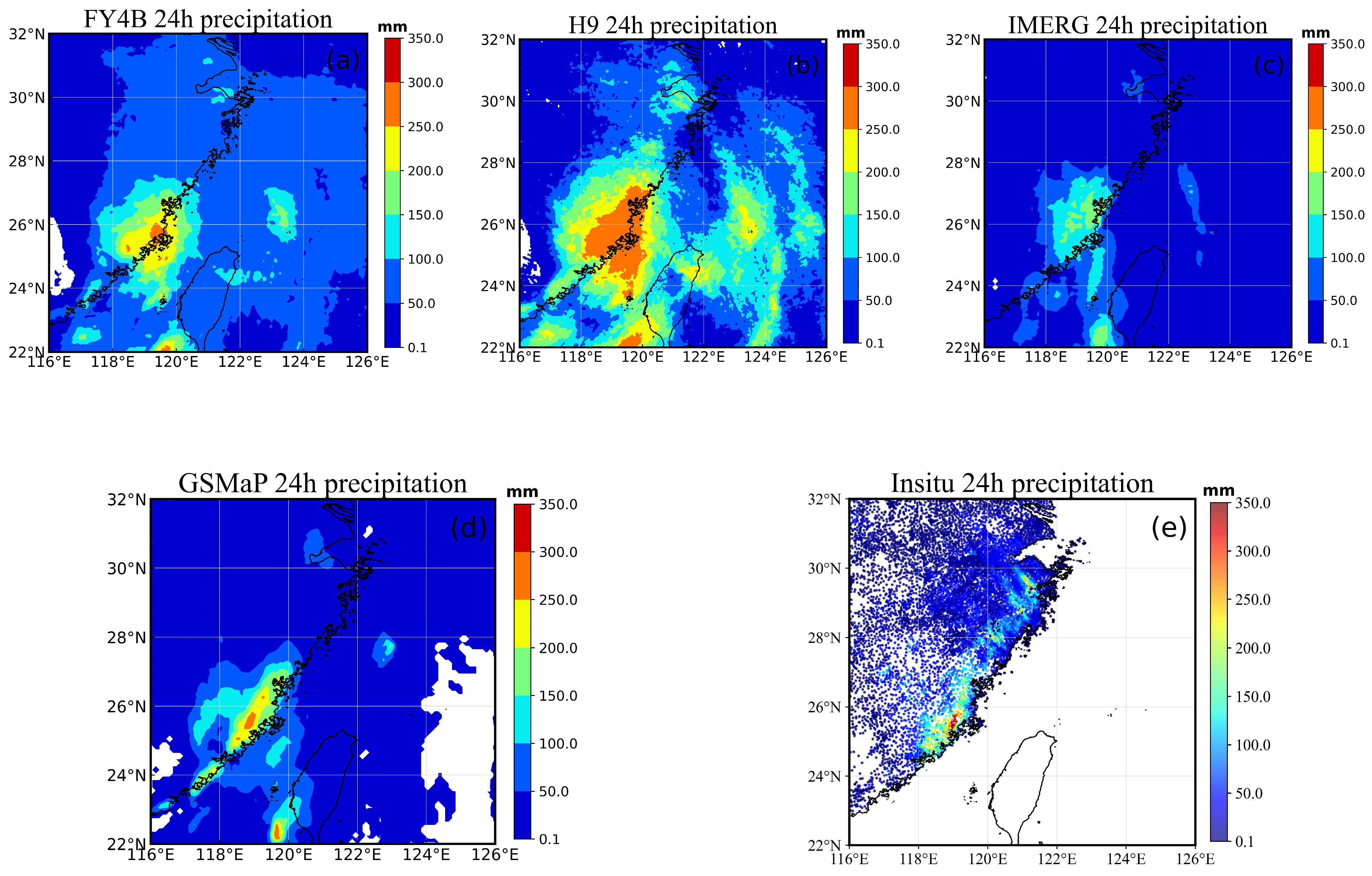
Compared to the 24-hour and 6-hour precipitation results, FY4B, H9, IMERG, and GSMaP performed relatively poorly in the 1 h rainfall analysis (see Table 3), with all scoring indicators showing a downward trend and a significant decrease. GSMaP and IMERG performed best at low-to-moderate-precipitation levels (<20 mm), while FY4B and H9 showed better performance in heavy rainfall (≥20 mm). The best performance was observed in light rainfall (>1 mm), where IMERG outperformed the others, with TS, ETS, CC, HSS, POD, and FAR values of 0.40, 0.36, 0.33, 0.52, 0.41, and 0.48, respectively. However, all four datasets showed the worst performance in extreme rainfall (>30 mm), with FY4B achieving the highest accuracy, with TS, ETS, CC, HSS, POD, and FAR values of 0.05, 0.05, 0.09, 0.09, 0.07, and 0.87, respectively.
Figure 4 illustrates the 1-hour precipitation error results for FY4B, H9, IMERG, and GSMaP. All four products (FY4B, H9, IMERG, GSMaP) show overestimation in the low-precipitation range (“0–1”, “1–5”), with FY4B and H9 also showing overestimation in the “5–10” range. In the precipitation ranges “10–20”, “20–30”, and “>30”, all products exhibit underestimation, with the most significant underestimation occurring in extreme precipitation (>30 mm), where GSMaP shows the largest underestimation (29.9). From the perspective of RMSE, the error for all products increases with higher precipitation. IMERG has the smallest error (0.6) in the low-precipitation range, while H9 has the largest error (2.1). Under extreme precipitation (>30 mm), GSMaP exhibits the highest error (31.5), while FY4B shows the lowest error (28.5).

3.2. A Case Study

Typhoon “Doksuri” formed in the northwest Pacific Ocean on the morning of 21 July 2023. It gradually intensified into a super typhoon, reaching its peak intensity (62 m per second) as recognized by the Central Meteorological Observatory on July 25. The typhoon made landfall on Fuga Island in the Philippines in the early morning of July 26, and by the evening of July 27, it was reclassified as a super typhoon. On the morning of July 28, it made landfall again along the coastal area of Jinjiang, Fujian Province, at a strong typhoon level. Subsequently, it weakened into a tropical depression in Anhui Province on July 29 and was declassified. However, its residual circulation continued moving northward, causing persistent heavy rainfall in northern China.
Typhoon “Doksuri” caused severe damage in both the Philippines and China. In the Philippines, its interaction with the southwest monsoon led to 30 fatalities and an economic loss of approximately PHP 15.318 billion. In China, the typhoon caused direct economic losses of CNY 14.95 billion across five provinces: Fujian, Zhejiang, Anhui, Jiangxi, and Guangdong. Its residual circulation resulted in 154 people being killed or declared missing, with economic losses totaling CNY 187.31 billion. The typhoon was later recognized as one of China’s top ten natural disasters and one of the top ten weather and climate events of 2023.
In this study, we apply the improved QPE algorithm to “Doksuri” and evaluate its effectiveness in assessing the heavy rainfall associated with the typhoon. We utilized meteorological station data from Fujian Province, China, on 28 August 2023 (UTC), to evaluate the algorithm’s performance in inverting typhoon landfall precipitation. A comparison between the inversion results and the actual observational data was conducted to assess the accuracy and reliability of the algorithm in predicting precipitation during typhoon landfall. Figure 5a shows the path of the super typhoon “Doksuri,” while Figure 5b,c presents the TBB distribution maps at landfall.

3.2.1. 24-Hour Precipitation Results

Table 4 presents the performance of FY4B, H9, IMERG, and GSMaP in typhoon landfall precipitation. We found that IMERG and GSMaP perform well under rainstorms and below (<100 mm), exhibiting significantly better TS, ETS, CC, HSS, and POD indicators than FY4B and H9. For example, at a precipitation level of 1 mm, the TS value for IMERG is 0.53, the ETS value is 0.47, and the CC value reaches 0.64. The HSS values for IMERG and GSMaP are 0.66 and 0.57, respectively, indicating their strong detection ability and correlation for moderate-to-low-intensity precipitation. Even at a precipitation level of 50 mm, the TS values (0.34 and 0.33) and ETS values (0.29) for IMERG and GSMaP remain superior to those of FY4B and H9 (TS values of 0.26 and 0.23, ETS values of 0.22 and 0.22, respectively). However, under heavy rainstorms or above (100 mm, 250 mm), FY4B and H9 perform better, particularly in the POD index. At a 100 mm precipitation level, the POD value for FY4B is 0.38, significantly higher than IMERG’s 0.36 and GSMaP’s 0.34, highlighting its stronger detection capability for heavy-rainstorm events. Additionally, the FAR values for FY4B and H9 are relatively low under heavy-precipitation conditions. For instance, FY4B has FAR values of 0.70 and 0.78 at the 100 mm and 250 mm precipitation levels, respectively, which are lower than GSMaP’s 0.82 and 0.86, further confirming their reliability under extreme-rainstorm scenarios.
FY4B, H9, IMERG, and GSMaP exhibit similar errors in the 24-hour typhoon landfall cumulative precipitation, as seen in the overall error analysis (see Figure 6). From a biased perspective, all four datasets show overestimation under heavy rain <25 mm and underestimation in heavy rain >25 mm. In terms of RMSE, GSMaP and IMERG exhibit smaller RMSE values in precipitation <100 mm compared to FY4B and H9. The four products show the smallest RMSE in the 0–1mm precipitation range, with IMERG having the smallest RMSE among them at 0.7. However, in rainstorms >100 mm, the errors for FY4B and H9 are smaller than those for GSMaP and IMERG, with the overall error being the largest in the >250 mm range. In this extreme-precipitation category, FY4B shows the smallest RMSE at 124.36.
We also compared the spatial distribution of the 24-hour precipitation results from FY4B, H9, IMERG, and GSMaP (see Figure 7). Compared to ground-based observations, FY4B, H9, and GSMaP show higher consistency in spatial distribution, especially in regions of intense precipitation during typhoon landfall, demonstrating greater accuracy. However, some underestimation still exists. In contrast, IMERG performs poorly in areas of heavy precipitation, with more significant underestimation and larger errors.

3.2.2. 6-Hour Precipitation Results

Regarding precipitation performance during typhoon landfall, the performance of FY4B, H9, IMERG, and GSMaP decreased compared to the 24-hour and overall precipitation assessment results (see Table 5). Overall, the performance trend remains the same, with IMERG and GSMaP performing the best under rainstorms <50 mm, while FY4B and H9 perform the best in rainfall ≥50 mm. For example, at a precipitation level of 1 mm, the TS value (0.52), CC value (0.53), and POD value (0.89) of IMERG are all the highest. At the levels of precipitation 50 mm and 100 mm, FY4B and H9 performed better, especially FY4B’s POD value (0.19 for 50 mm), which was significantly higher than IMERG and GSMaP, while its FAR value was lower (0.72 for 50 mm), indicating its stronger ability to detect heavy precipitation.
We also compared the precipitation errors of FY4B, H9, IMERG, and GSMaP during typhoon landfall and found that the errors were higher (see Figure 8). All four products (FY4B, H9, IMERG, and GSMaP) overestimate precipitation in the “0–1” and “1–5” mm ranges, while FY4B and H9 overestimate and IMERG and GSMaP underestimate precipitation in the “5–10” mm range. For precipitation levels greater than 10 mm, all products (FY4B, H9, IMERG, and GSMaP) show underestimation. From the perspective of RMSE, it increases as precipitation levels rise. Under the rainstorm ranges <50 mm, IMERG and GSMaP have lower RMSE values than FY4B and H9, with GSMaP achieving the smallest RMSE of 1.0 in the “0–1 mm” range. However, in the rainstorm ranges >50 mm, IMERG and GSMaP show higher RMSE values than FY4B and H9, with FY4B exhibiting the smallest RMSE at 94.96 in the “>100 mm” range.
Compared to the 24-hour precipitation results, the spatial distribution of 6-hour precipitation shows some limitations (see Figure 9). This is particularly evident in areas of heavy precipitation, where both FY4B and H9 exhibit noticeable underestimation compared to station-measured precipitation. Despite these discrepancies, FY4B and H9 still perform relatively closely to the observed values. In contrast, IMERG and GSMaP show more significant estimation errors.

4. Discussion

Geostationary satellites, due to their fixed positions, provide high temporal resolution data through continuous observations of the Earth [31]. This continuous observation capability makes monitoring the temporal and spatial changes in precipitation more feasible, which is particularly useful for capturing intense precipitation events over short periods and for timely updates to weather forecasts [32]. Geostationary satellite data can typically be processed and transmitted to the ground within minutes of observation, providing near-real-time precipitation information. This is crucial for disaster warnings and responses, such as the timely forecasting and handling of typhoons, heavy rains, and other severe weather events.
In this study, we designed a correction equation construction method to address the imbalance between heavy-rainfall and light-rainfall samples. In the original dataset, heavy-rainfall events are relatively rare, which weakens the model’s ability to identify heavy rainfall. To resolve this issue, we balanced the number of heavy-rainfall and light-rainfall samples by resampling the data, ensuring an equal number of both. This correction step aims to allow the model to fully learn the characteristics of heavy rainfall and thus improve its performance under extreme weather conditions. This strategy significantly enhanced the performance of the FY-4B and H9 models during training, particularly in predicting extreme heavy-rainfall events. By balancing the class distribution in the dataset, the model was better able to identify and predict heavy-rainfall events, resulting in a stronger performance in threat Score (TS) and equitable threat score (ETS).
This study demonstrates that using geostationary satellite cloud top brightness temperatures to estimate precipitation can effectively address the spatial limitations of station data, particularly in areas with sparse stations and over oceans. However, it is essential to note that the method used in this study has some limitations. Since this study relies on cloud top brightness temperatures in the near-infrared spectrum, which cannot penetrate cloud layers and can only observe radiative information from the cloud top, direct observation of precipitation below the clouds is impossible [33]. This means that in cases of thick or multilayered clouds, near-infrared data cannot provide accurate information about surface precipitation. Additionally, this method does not capture internal cloud temperatures, humidity, and precipitation distribution, limiting the understanding of cloud microphysical properties and precipitation mechanisms. Moreover, the near-infrared spectrum exhibits significant differences in observation quality between day and night. During the day, solar radiation increases the near-infrared reflectance, while at night, near-infrared radiation is weaker. This diurnal variation reduces the consistency of near-infrared data in all-weather monitoring.
The intrinsic systematic errors of satellite data—such as cloud thickness, atmospheric conditions, solar angle, and the calibration errors of the satellite sensors themselves—are major contributors to the inaccuracies in quantitative precipitation estimation (QPE) algorithms [18,34]. Additionally, the correction fusion algorithm used in this study is based on regression analysis with large samples, and various factors such as the distribution of observation stations and differences in satellite data can influence the algorithm to varying degrees. The number of samples and time can also lead to errors, and using existing typhoon data to estimate the heavy precipitation of future typhoons is biased, which is also one of the shortcomings of this algorithm. For example, complex factors such as strong convective activity during precipitation, microphysical processes, and local topographical effects can lead to significant deviations between the retrieved results and actual precipitation [35]. Furthermore, the accuracy of QPE algorithms can vary when dealing with different types of precipitation (e.g., convective versus stratiform precipitation), presenting challenges for the generalizability of results [36,37]. Finally, this study did not fully consider the changes in precipitation characteristics across different time scales. Satellite-derived precipitation represents instantaneous precipitation, and rapid changes in actual precipitation processes can lead to significant instantaneous errors in retrievals.
The results of the 6-hour and 1-hour precipitation analyses are not as good as those of the 24-hour precipitation, mainly because precipitation at short time scales (such as 1 h and 6 h) has higher spatiotemporal variability. Specifically, precipitation over short periods exhibits large fluctuations in spatial distribution and intensity, which are significantly influenced by local climatic factors (such as topography, local convection, etc.), making it challenging for models to capture these rapid changes accurately. Additionally, observational data at short time scales are usually sparser, especially in satellite remote sensing, where capturing short-term precipitation can be limited by cloud coverage and observation frequency, leading to less accurate predictions compared to longer periods.
In summary, there are still some shortcomings in this study, and future work will include continuing to improve satellite typhoon precipitation monitoring, adding polar orbit satellites to supplement the disadvantage of stationary satellites not being able to penetrate clouds, and also consider using machine learning methods to further improve and optimize the correction fusion algorithm to achieve more accurate and reliable satellite precipitation estimation.

5. Conclusions

This study has optimized and improved the QPE precipitation estimation algorithm of Adler and Negri based on Himawari-9 and FY4B satellite TBB data and proposed a precipitation correction scheme based on geostationary satellites. Additionally, using the rain gauge data from mainland China, the study has analyzed and compared the datasets of IMERG, GSMaP, and both new FY4B-TBB and H9-TBB satellite-derived precipitation in capturing 1-hour, 6-hour, and 24-hour precipitation events associated with a landfalling typhoon over mainland China.
The results indicate that the new QPE algorithm based on the FY4B and H9 satellites has largely improved the precipitation estimation capability, especially for heavy-precipitation conditions. By comparing and analyzing the precipitation performance of FY4B, H9, IMERG, and GSMaP at different time scales (1 h, 6 h, and 24 h), it can be concluded that under extreme heavy-precipitation conditions, FY4B and H9 performed better, especially in terms of the POD index and false alarm rate (FAR), indicating their stronger detection ability in heavy-precipitation events. FY4B had the smallest error, demonstrating its advantage in extreme-precipitation scenarios. Therefore, IMERG and GSMaP perform well in low-to-moderate-intensity precipitation, while FY4B and H9 have more advantages under high-intensity precipitation conditions, providing important references for satellite product selection under different precipitation conditions. We also found that compared to the 6-hour estimate, these three satellite products have better accuracy in estimating 24-hour rainfall, and the 6-hour estimate is more accurate than the 1-hour estimate. IMERG and GSMaP perform better at low-to-moderate-precipitation intensities, with smaller RMSEs and higher scoring indicators (such as TS, ETS, CC, HSS). Especially under mild-precipitation conditions, IMERG performs the best.
In summary, the QPE algorithm with the newly proposed correction scheme in this study can effectively improve the heavy-precipitation retrieval capabilities of the high-resolution geostationary satellites of FY4B and H9, making satellite precipitation estimates more reliable for monitoring and forecasting severe weather events such as typhoons.

Author Contributions

Conceptualization, H.C. and Z.Y.; methodology, H.C.; software, H.C.; validation, H.C.; formal analysis, H.C.; investigation, H.C. and Z.Y.; resources, Z.Y.; data curation, H.C.; writing—original draft preparation, H.C.; writing—review and editing, H.C., Z.Y., Y.Y. and R.R.; visualization, H.C.; supervision, Z.Y.; project administration, Z.Y.; funding acquisition, Z.Y. All authors have read and agreed to the published version of the manuscript.

Funding

This study was supported by the Shanghai Science and Technology Commission Fund [No. 23DZ1204700], Ningbo Key R&D Program [No. 2023Z139], and the Shanghai Meteorological Service Qimingxing Project [No. QM202517].

Data Availability Statement

The original contributions presented in the study are included in the article, further inquiries can be directed to the corresponding author.

Acknowledgments

The data that support the findings of this study are available, open, and free to the public and can be downloaded from the websites presented in Section 2 “Materials and Methods”.

Conflicts of Interest

The authors declare no conflicts of interest.

Appendix A

Evaluation metric calculation formulas:
T S = H H + F + M
C H = ( H + M ) ( H + F ) H + F + M + Z
E T S = H C H H + F + M C H
H S S = 2 H × Z F × M H + M M + Z + H + F F + Z
C C = i = 1 N Y i Y ¯ X i X ¯ i = 1 N Y i Y 2 i = 1 N X i X 2
P O D = H H + F
F A R = M H + M
B i a s = 1 N i = 1 N Y i X i
R M S E = 1 N i = 1 N Y i X i 2
where Z represents observed no rainfall with model no rainfall; F indicates observed no rainfall but model rainfall; M represents observed rainfall but model no rainfall; and H indicates observed rainfall with model rainfall.  Y i  is the observed value at the station,  X i  is the inverted value,  Y ¯  is the mean of the station results, and  X ¯  is the mean of the inverted results.

References

  1. Markonis, Y.; Papalexiou, S.M.; Martinkova, M.; Hanel, M. Assessment of Water Cycle Intensification Over Land using a Multisource Global Gridded Precipitation DataSet. J. Geophys. Res. Atmos. 2019, 124, 11175–11187. [Google Scholar] [CrossRef]
  2. Zhou, Z.; Guo, B.; Xing, W.; Zhou, J.; Xu, F.; Xu, Y. Comprehensive evaluation of latest GPM era IMERG and GSMaP precipitation products over mainland China. Atmos. Res. 2020, 246, 105132. [Google Scholar] [CrossRef]
  3. Braithwaite, D.K.; Sorooshian, S.; Hsu, K.-L.; Ashouri, H.; Knapp, K.R.; Cecil, L.D.; Nelson, B.R.; Prat, O.P. PERSIANN-CDR: Daily Precipitation Climate Data Record from Multisatellite Observations for Hydrological and Climate Studies. Bull. Am. Meteorol. Soc. 2015, 96, 69–83. [Google Scholar] [CrossRef]
  4. Huffman, G.J.; Adler, R.F.; Bolvin, D.T.; Gu, G. Improving the global precipitation record: GPCP Version 2.1. Geophys. Res. Lett. 2009, 36. [Google Scholar] [CrossRef]
  5. Sharifi, E.; Saghafian, B.; Steinacker, R. Downscaling Satellite Precipitation Estimates With Multiple Linear Regression, Artificial Neural Networks, and Spline Interpolation Techniques. J. Geophys. Res. Atmos. 2019, 124, 789–805. [Google Scholar] [CrossRef]
  6. Shen, Y.; Xiong, A.; Hong, Y.; Yu, J.; Pan, Y.; Chen, Z.; Saharia, M. Uncertainty analysis of five satellite-based precipitation products and evaluation of three optimally merged multi-algorithm products over the Tibetan Plateau. Int. J. Remote Sens. 2014, 35, 6843–6858. [Google Scholar] [CrossRef]
  7. Nguyen, P.; Ombadi, M.; Sorooshian, S.; Hsu, K.; AghaKouchak, A.; Braithwaite, D.; Ashouri, H.; Thorstensen, A.R. The PERSIANN family of global satellite precipitation data: A review and evaluation of products. Hydrol. Earth Syst. Sci. 2018, 22, 5801–5816. [Google Scholar] [CrossRef]
  8. Yang, Z.; Hsu, K.; Sorooshian, S.; Xu, X.; Braithwaite, D.; Zhang, Y.; Verbist, K.M.J. Merging high-resolution satellite-based precipitation fields and point-scale rain gauge measurements—A case study in Chile. J. Geophys. Res. Atmos. 2017, 122, 5267–5284. [Google Scholar] [CrossRef]
  9. Zhang, M.; Luo, C.; Zou, Y. A Model for Quantitatively Estimating Short-Range Precipitation Based on GMS Digitalized Cloud Maps-Part I: Analysis of Quantitative Cloud-Precipitation Relations and Model Design. ACTA Meteorol. Sin.-Engl. Ed. 2003, 17, 230–244. [Google Scholar]
  10. Jiang, S.; Wei, L.; Ren, L.; Xu, C.-Y.; Zhong, F.; Wang, M.; Zhang, L.; Yuan, F.; Liu, Y. Utility of integrated IMERG precipitation and GLEAM potential evapotranspiration products for drought monitoring over mainland China. Atmos. Res. 2021, 247, 105141. [Google Scholar] [CrossRef]
  11. Wei, L.; Jiang, S.; Ren, L.; Zhang, L.; Wang, M.; Duan, Z. Preliminary utility of the retrospective IMERG precipitation product for large-scale drought monitoring over Mainland China. Remote Sens. 2020, 12, 2993. [Google Scholar] [CrossRef]
  12. Hsu, K.-l.; Gao, X.; Sorooshian, S.; Gupta, H.V. Precipitation estimation from remotely sensed information using artificial neural networks. J. Appl. Meteorol. Climatol. 1997, 36, 1176–1190. [Google Scholar] [CrossRef]
  13. Hong, Y.; Hsu, K.-L.; Sorooshian, S.; Gao, X. Precipitation estimation from remotely sensed imagery using an artificial neural network cloud classification system. J. Appl. Meteorol. 2004, 43, 1834–1853. [Google Scholar] [CrossRef]
  14. Yue, C.-j.; Chen, P.; Lei, X.-t.; Yang, Y. A preliminary study on method of Quantitative Precipitation Estimation (QPE) for landfall typhoon. Sci. Meteor. Sin 2006, 26, 17–23. [Google Scholar]
  15. Ma, Z.; Zhu, S.; Yang, J. FY4QPE-MSA: An all-day near-real-time quantitative precipitation estimation framework based on multispectral analysis from AGRI onboard Chinese FY-4 series satellites. IEEE Trans. Geosci. Remote Sens. 2022, 60, 1–15. [Google Scholar] [CrossRef]
  16. Min, M.; Bai, C.; Guo, J.; Sun, F.; Liu, C.; Wang, F.; Xu, H.; Tang, S.; Li, B.; Di, D. Estimating summertime precipitation from Himawari-8 and global forecast system based on machine learning. IEEE Trans. Geosci. Remote Sens. 2018, 57, 2557–2570. [Google Scholar] [CrossRef]
  17. Sehad, M.; Lazri, M.; Ameur, S. Novel SVM-based technique to improve rainfall estimation over the Mediterranean region (north of Algeria) using the multispectral MSG SEVIRI imagery. Adv. Space Res. 2017, 59, 1381–1394. [Google Scholar] [CrossRef]
  18. Wang, C.; Tang, G.; Xiong, W.; Ma, Z.; Zhu, S. Infrared Precipitation Estimation using Convolutional neural network for FengYun satellites. J. Hydrol. 2021, 603, 127113. [Google Scholar] [CrossRef]
  19. Wang, X.; Ding, Y.; Zhao, C.; Wang, J. Similarities and improvements of GPM IMERG upon TRMM 3B42 precipitation product under complex topographic and climatic conditions over Hexi region, Northeastern Tibetan Plateau. Atmos. Res. 2019, 218, 347–363. [Google Scholar] [CrossRef]
  20. Wang, W.; Lu, H.; Zhao, T.; Jiang, L.; Shi, J. Evaluation and Comparison of Daily Rainfall From Latest GPM and TRMM Products Over the Mekong River Basin. IEEE J. Sel. Top. Appl. Earth Obs. Remote Sens. 2017, 10, 2540–2549. [Google Scholar] [CrossRef]
  21. Zhang, C.; Chen, X.; Shao, H.; Chen, S.; Liu, T.; Chen, C.; Ding, Q.; Du, H. Evaluation and Intercomparison of High-Resolution Satellite Precipitation Estimates—GPM, TRMM, and CMORPH in the Tianshan Mountain Area. Remote Sens. 2018, 10, 1543. [Google Scholar] [CrossRef]
  22. Yu, Z.; Yu, H.; Chen, P.; Qian, C.; Yue, C. Verification of tropical cyclone–related satellite precipitation estimates in mainland China. J. Appl. Meteorol. Climatol. 2009, 48, 2227–2241. [Google Scholar] [CrossRef]
  23. Adler, R.F.; Negri, A.J. A satellite infrared technique to estimate tropical convective and stratiform rainfall. J. Appl. Meteorol. Climatol. 1988, 27, 30–51. [Google Scholar] [CrossRef]
  24. Goldenbergl, S.B.; Houze, R.A., Jr.; Churchill, D.D. Convective and stratiform components of a winter monsoon cloud cluster determined from geosynchronous infrared satellite data. J. Meteorol. Soc. Jpn. Ser. II 1990, 68, 37–63. [Google Scholar] [CrossRef]
  25. Beattie, C.; Leibo, J.Z.; Teplyashin, D.; Ward, T.; Wainwright, M.; Küttler, H.; Lefrancq, A.; Green, S.; Valdés, V.; Sadik, A. Deepmind lab. arXiv 2016, arXiv:1612.03801. [Google Scholar]
  26. Huffman, G.J.; Bolvin, D.T.; Braithwaite, D.; Hsu, K.; Joyce, R.; Xie, P.; Yoo, S.-H. NASA global precipitation measurement (GPM) integrated multi-satellite retrievals for GPM (IMERG). Algorithm Theor. Basis Doc. (ATBD) Vers. 2015, 4, 30. [Google Scholar]
  27. Wang, Y.; Li, Z.; Gao, L.; Zhong, Y.; Peng, X. Comparison of GPM IMERG version 06 final run products and its latest version 07 precipitation products across scales: Similarities, differences and improvements. Remote Sens. 2023, 15, 5622. [Google Scholar] [CrossRef]
  28. Tian, Y.; Peters-Lidard, C.D.; Adler, R.F.; Kubota, T.; Ushio, T. Evaluation of GSMaP precipitation estimates over the contiguous United States. J. Hydrometeorol. 2010, 11, 566–574. [Google Scholar] [CrossRef]
  29. Prakash, S.; Mitra, A.K.; Rajagopal, E.; Pai, D. Assessment of TRMM-based TMPA-3B42 and GSMaP precipitation products over India for the peak southwest monsoon season. Int. J. Climatol. 2016, 36, 1614–1631. [Google Scholar] [CrossRef]
  30. Li, J.; Wang, L.; Zhou, F. Convective and stratiform cloud rainfall estimation from geostationary satellite data. Adv. Atmos. Sci. 1993, 10, 475–480. [Google Scholar] [CrossRef]
  31. Yin, G.; Baik, J.; Park, J. Comprehensive analysis of GEO-KOMPSAT-2A and FengYun satellite-based precipitation estimates across Northeast Asia. GIScience Remote Sens. 2022, 59, 782–800. [Google Scholar] [CrossRef]
  32. Sun, Q.; Miao, C.; Duan, Q.; Ashouri, H.; Sorooshian, S.; Hsu, K.L. A review of global precipitation data sets: Data sources, estimation, and intercomparisons. Rev. Geophys. 2018, 56, 79–107. [Google Scholar] [CrossRef]
  33. Scofield, R.A.; Kuligowski, R.J. Status and outlook of operational satellite precipitation algorithms for extreme-precipitation events. Weather Forecast. 2003, 18, 1037–1051. [Google Scholar] [CrossRef]
  34. Gao, Z.; Huang, B.; Ma, Z.; Chen, X.; Qiu, J.; Liu, D. Comprehensive comparisons of state-of-the-art gridded precipitation estimates for hydrological applications over southern China. Remote Sens. 2020, 12, 3997. [Google Scholar] [CrossRef]
  35. Basist, A.; Bell, G.D.; Meentemeyer, V. Statistical relationships between topography and precipitation patterns. J. Clim. 1994, 7, 1305–1315. [Google Scholar] [CrossRef]
  36. Upadhyaya, S.A.; Kirstetter, P.-E.; Gourley, J.J.; Kuligowski, R.J. On the propagation of satellite precipitation estimation errors: From passive microwave to infrared estimates. J. Hydrometeorol. 2020, 21, 1367–1381. [Google Scholar] [CrossRef]
  37. Vicente, G.A.; Scofield, R.A.; Menzel, W.P. The operational GOES infrared rainfall estimation technique. Bull. Am. Meteorol. Soc. 1998, 79, 1883–1898. [Google Scholar] [CrossRef]
Figure 1. Spatial distribution of ground meteorological stations across China.
Remotesensing 17 01703 g001
Figure 2. 24-hour precipitation error results.: (a) bias; (b) RMSE. Unit: mm.
Remotesensing 17 01703 g002
Figure 3. 6-hour precipitation error results: (a) bias; (b) RMSE. Unit: mm.
Remotesensing 17 01703 g003
Figure 4. 1-hour precipitation error results: (a) bias; (b) RMSE. Unit: mm.
Remotesensing 17 01703 g004
Figure 5. Path of super typhoon “Doksuri” landfall and cloud top brightness temperature results: (a) track of “Doksuri”, (b) TBB distribution map from FY4B at landfall, and (c) TBB distribution map from H9 at landfall. The landfall time was 2:00 AM UTC on 28 July.
Remotesensing 17 01703 g005
Figure 6. 24-hour typhoon landfall precipitation error results: (a) bias; (b) RMSE. Unit: mm.
Remotesensing 17 01703 g006
Figure 7. 24-hour accumulated precipitation spatial distribution results: (a) FY4B; (b) H9; (c) IMERG; (d) GSMaP; (e) In situ.
Remotesensing 17 01703 g007
Figure 8. 6-hour typhoon landfall precipitation error results: (a) bias; (b) RMSE. Unit: mm.
Remotesensing 17 01703 g008
Figure 9. 6-hour accumulated precipitation spatial distribution results: (a) FY4B; (b) H9; (c) IMERG; (d) GSMaP; (e) In situ.
Remotesensing 17 01703 g009
Table 1. 24-hour rainfall estimate performance of FY4B, H9, IMERG, and GSMaP.
1102550100250
TSFY4B0.420.390.360.330.300.15
H90.450.420.350.310.280.11
IMERG0.540.510.470.360.270.13
GSMaP0.520.470.460.350.250.13
ETSFY4B0.380.340.330.290.270.15
H90.340.340.310.260.230.11
IMERG0.480.410.400.340.210.11
GSMaP0.420.390.380.330.160.11
CCFY4B0.660.620.570.520.360.25
H90.670.650.610.490.340.22
IMERG0.730.690.620.580.400.18
GSMaP0.720.670.600.500.360.12
HSSFY4B0.440.390.380.430.310.28
H90.510.510.480.420.320.19
IMERG0.670.630.600.550.360.18
GSMaP0.590.560.550.550.280.17
PODFY4B0.800.740.650.540.440.19
H90.800.680.610.490.310.11
IMERG0.850.820.780.560.420.16
GSMaP0.820.790.760.530.360.14
FARFY4B0.360.360.490.500.520.62
H90.260.390.440.520.540.65
IMERG0.200.360.410.450.540.63
GSMaP0.220.380.410.440.580.66
Table 2. 6-hour rainfall estimate performance of FY4B, H9, IMERG, and GSMaP.
1102550100
TSFY4B0.400.260.220.200.14
H90.420.310.210.170.08
IMERG0.480.390.330.170.08
GSMaP0.480.350.280.140.06
ETSFY4B0.330.270.220.200.14
H90.370.300.220.160.08
IMERG0.390.330.320.170.08
GSMaP0.390.320.270.140.06
CCFY4B0.380.310.250.130.11
H90.380.330.250.120.06
IMERG0.510.420.330.120.06
GSMaP0.480.370.280.110.04
HSSFY4B0.460.360.340.330.16
H90.520.420.320.280.11
IMERG0.560.480.430.260.11
GSMaP0.560.480.420.240.11
PODFY4B0.820.490.380.280.16
H90.820.490.360.240.11
IMERG0.880.620.540.260.11
GSMaP0.840.560.400.230.11
FARFY4B0.430.530.600.630.71
H90.420.520.600.620.74
IMERG0.300.380.410.620.76
GSMaP0.330.430.480.670.79
Table 3. 1-hour rainfall estimate performance of FY4B, H9, IMERG, and GSMaP.
15102030
TSFY4B0.300.160.100.080.05
H90.340.170.110.060.04
IMERG0.400.220.170.060.04
GSMaP0.380.190.140.050.04
ETSFY4B0.270.150.090.080.05
H90.270.170.100.060.04
IMERG0.360.210.140.040.04
GSMaP0.340.180.110.040.03
CCFY4B0.260.210.180.110.09
H90.270.230.180.100.08
IMERG0.330.270.240.100.08
GSMaP0.280.240.190.090.07
HSSFY4B0.390.300.170.110.09
H90.420.300.190.080.08
IMERG0.520.410.280.100.07
GSMaP0.510.320.200.080.07
PODFY4B0.370.240.200.090.07
H90.360.250.210.050.05
IMERG0.410.340.270.050.04
GSMaP0.400.310.270.050.02
FARFY4B0.650.730.830.850.87
H90.630.690.810.880.90
IMERG0.480.590.740.890.90
GSMaP0.500.630.800.910.95
Table 4. 24-hour landfall TC rainfall estimate performance of FY4B, H9, IMERG, and GSMaP.
1102550100250
TSFY4B0.460.390.330.260.200.18
H90.460.340.320.230.190.18
IMERG0.530.470.440.340.180.14
GSMaP0.510.460.440.330.160.09
ETSFY4B0.370.330.270.220.200.18
H90.380.350.240.220.180.17
IMERG0.440.410.350.290.150.12
GSMaP0.400.380.300.290.130.07
CCFY4B0.670.500.440.410.380.26
H90.560.470.390.370.330.20
IMERG0.640.620.610.560.330.19
GSMaP0.610.600.580.530.320.15
HSSFY4B0.480.400.340.320.220.20
H90.470.370.320.280.210.20
IMERG0.660.630.520.480.220.14
GSMaP0.570.550.500.450.220.13
PODFY4B0.860.760.610.400.380.21
H90.870.650.570.480.360.19
IMERG0.930.900.810.580.360.18
GSMaP0.900.820.700.490.340.17
FARFY4B0.340.360.390.680.700.78
H90.300.320.430.670.710.80
IMERG0.220.260.320.600.740.82
GSMaP0.260.280.410.630.820.86
Table 5. 6-hour landfall TC rainfall estimate performance of FY4B, H9, IMERG, and GSMaP.
1102550100
TSFY4B0.440.330.240.180.15
H90.450.320.200.120.10
IMERG0.520.480.270.220.09
GSMaP0.510.460.260.220.06
ETSFY4B0.360.260.220.180.15
H90.360.240.190.120.10
IMERG0.410.320.270.220.09
GSMaP0.390.290.260.220.06
CCFY4B0.350.290.210.160.12
H90.400.270.190.160.13
IMERG0.530.370.310.180.12
GSMaP0.480.320.290.140.09
HSSFY4B0.510.370.360.280.20
H90.530.330.310.260.18
IMERG0.560.510.480.330.12
GSMaP0.560.530.460.360.08
PODFY4B0.800.440.300.190.17
H90.830.390.260.150.16
IMERG0.890.510.440.140.11
GSMaP0.870.480.360.140.06
FARFY4B0.420.580.640.720.81
H90.440.570.680.750.85
IMERG0.230.450.590.760.86
GSMaP0.250.540.610.790.89
Disclaimer/Publisher’s Note: The statements, opinions and data contained in all publications are solely those of the individual author(s) and contributor(s) and not of MDPI and/or the editor(s). MDPI and/or the editor(s) disclaim responsibility for any injury to people or property resulting from any ideas, methods, instructions or products referred to in the content.

