Simultaneous Vibration and Nonlinearity Compensation for One-Period Triangular FMCW Ladar Signal Based on MSST

Abstract

When frequency-modulated continuous-wave (FMCW) laser radar (Ladar) is employed for three-dimensional imaging, the echo signal is susceptible to modulation nonlinearity and platform vibration due to modulation and the short wavelength. These effects cause main-lobe widening, side-lobe elevation, and positional shift, which degrades distance detection accuracy. To solve these problems, this paper proposes a compensation method combining multiple synchrosqueezing transform (MSST), equal-phase interval resampling, and high-order ambiguity function (HAF). Firstly, variational mode decomposition (VMD) is applied to the optical prism signal to eliminate low-frequency noise and harmonic peaks. MSST is used to extract the time–frequency curve of the optical prism. The nonlinearity in the transmitted signal is estimated by two-step integration. An internal calibration signal containing nonlinearity is constructed at a higher sampling rate to resample the actual signal at an equal-phase interval. Then, HAF compensates for high-order vibration and residual phase error after resampling. Finally, symmetrical triangle wave modulation is used to remove constant-speed vibration. Verifying by actual data, the proposed method can enhance the main lobe and suppress the side lobe about 1.5 dB for a strong reflection target signal. Natural-target peaks can also be enhanced and the remaining peaks are suppressed, which is helpful to extract an accurate target distance.

1. Introduction

Frequency-modulated continuous-wave (FMCW) laser radar (Ladar) combines electronic frequency modulation, optical coherence, and radar signal processing, which makes it a technology with growing research and promising application interest [1]. Compared with traditional pulse Ladar, which measures optical time-of-flight (ToF) for distance measurement, FMCW Ladar uses optical heterodyne detection to establish a connection between target distance and signal frequency, enabling high-precision ranging. Due to the continuous-wave system, it can work at a lower power [2]. FMCW Ladar provides more continuous ground observations and an enhanced detection of faint targets compared to pulsed systems. However, system structure change also introduces problems, primarily frequency modulation nonlinearity and platform vibration. Nonlinearity leads to main-lobe widening, side-lobe elevation, peak distortion, and positional shifts [3], all of which degrade the ranging accuracy and point cloud quality. Additionally, Ladar works in the infrared band, and the short wavelength amplifies the influence of the Doppler effect, causing large frequency deviation from the small platform vibration, further affecting range accuracy and distorting point cloud targets [4]. Since FMCW Ladar has a large bandwidth and works on a moving platform, these issues usually co-exist. When FMCW Ladar generates a point cloud, each period represents a laser footprint and there are no repeated observations. There is no azimuth concept in synthetic aperture radar (SAR) or long-dwell observation in frequency scanning interferometry (FSI). Thus, the problem is summarized as the compensation for frequency modulation nonlinearity and platform vibration in one period.

Only a few of the existing literatures discuss the simultaneous compensation of the two errors. Wang et al. use second-order SST to extract the time–frequency variation curve and derives range expression for joint vibration-nonlinearity disturbance. Nonlinearity is extracted from a reference signal and directly compensated, while the particle filter is used to compensate for high-order vibration [5]. Although this method achieves simultaneous compensation, it is not accurate to directly compensate for nonlinearity extracted from the reference signal into the target dechirp signal, and the particle filter’s vibration tracking is highly sensitive to phase noise. Song et al. unify the nonlinearity and vibration into a polynomial model, jointly analyzing them and compensating coefficients step-by-step using discrete polynomial transformation [6]. However, this method suffers from error accumulation, limiting its effectiveness. Zhang et al. use equal-phase interval resampling to compensate for nonlinearity and use symmetrical triangle wave modulation to compensate for vibration. This method is a simple combination of the two compensation methods, which has a requirement of reference signal delay and only models the vibration at a constant speed [7].

Among the methods for compensating frequency modulation nonlinearity, in addition to hardware improvement methods, data processing methods such as residual video-phase (RVP) filtering and equal-phase interval resampling are widely used. The RVP filter method is particularly notable for its ability to compensate multi-target echoes with unknown time delays by making the nonlinear phase independent of target delay, enabling a uniform compensation [8]. However, its application requires a reference signal with a known small delay to estimate a transmitted signal’s nonlinearity. Since the estimation relies on first-order Taylor expansion, smaller delay results better the compensation. A number of improvements to the RVP filter method have been proposed. Yang et al. introduce a comb notch filter applied to the reference signal. 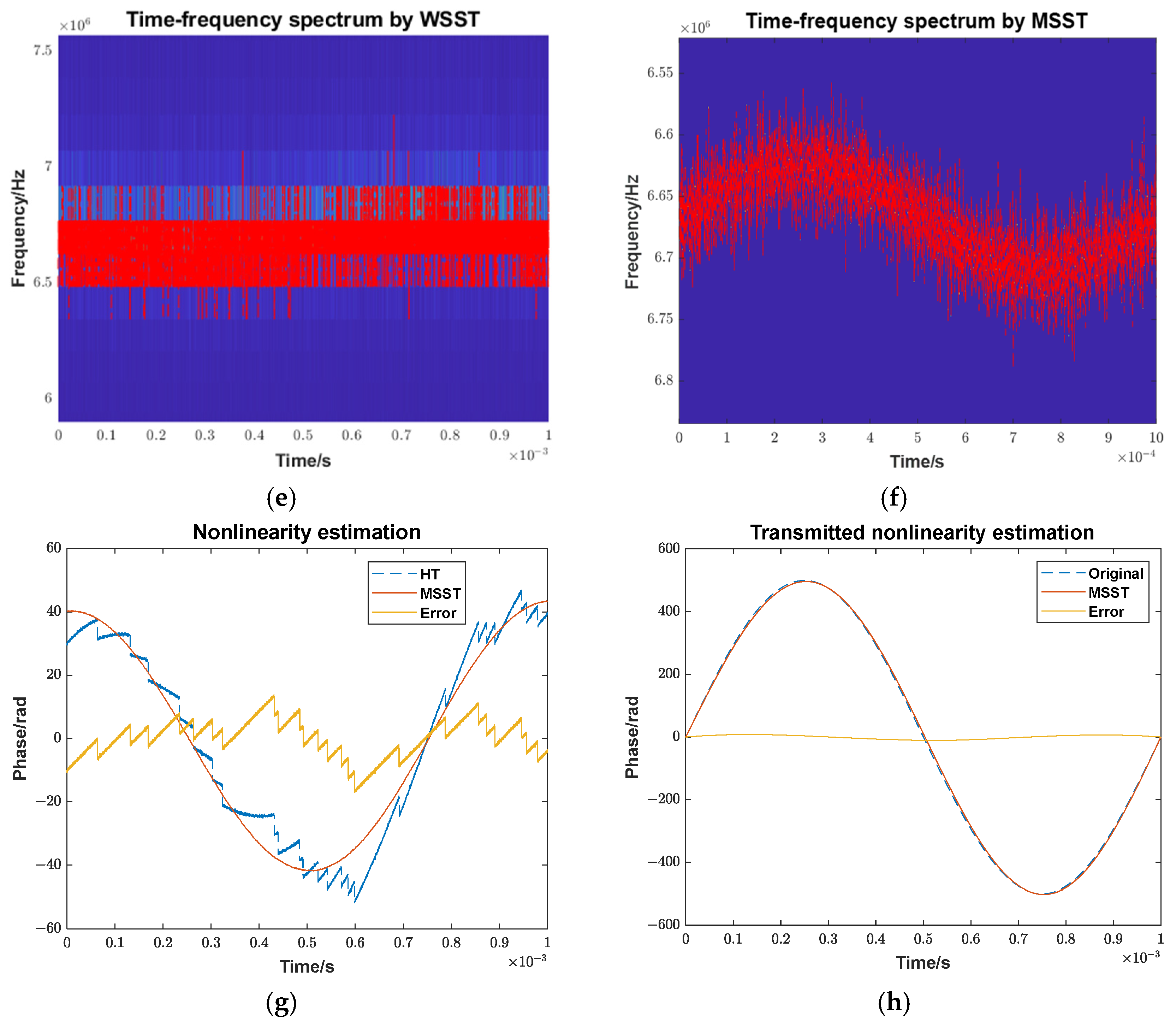The nonlinear phase is generated by reference target and its harmonics, leading to a more accurate transmitted nonlinearity estimation [9]. Wang et al. combine the RVP filter with wavelet synchro-squeezing transforms (WSST). Compared with using Hilbert transform (HT) to extract the phase, WSST can reduce phase-noise influence due to its energy aggregation characteristic, robustly extract the time–frequency curve, and improve nonlinearity estimation accuracy [10]. Li et al. estimate transmitted nonlinearity by using two strong echo signals with known delays as reference signals, combined with the phase gradient autofocus (PGA) method and remove nonlinearity using an RVP filter [11]. Chu et al. model nonlinearity as a sum of polynomial and sinusoidal components. After estimating transmitted nonlinearity, the coefficients of the polynomial and sinusoidal models are estimated, followed by the RVP filter [12]. While the method is very accurate in deriving the model, the RVP method itself does not heavily rely on specific model coefficients. From these improvements, it can be seen that the RVP filter method is the core of de-nonlinearity and their improvement strategies are mostly based on a more accurate transmitted nonlinearity estimation. The core requirement is a reference signal with a known time delay.

The equal-phase interval resampling method uses a reference signal with a known time delay to resample the target signal by replacing the equal time axis with an equal phase axis. The purpose is to convert the high-order phase of the original signal with respect to time into a linear expression with respect to phase, ensuring that its first-order derivative is still the point frequency, thereby eliminating the effects of nonlinearity [13]. Many improvements have been proposed to enhance this method: Ahn et al. use HT to extract the phase from a reference signal with a known time delay, and removes nonlinearity by equal-phase interval resampling [14]. While straightforward, this method is limited by phase noise, which reduces the accuracy of the extracted phase. Lin et al. reduce the equal-phase interval from π to a shorter value, avoiding the limitation that the reference fiber delay must exceed twice the actual target distance [15]. Zhang et al. also propose a similar method, dividing multiple equal phase points based on the phase zero crossing point [16]. However, shorter interval increase the susceptibility to phase noise. Zheng et al. consider the reference signal with multiple peaks, applying complementary ensemble empirical mode decomposition (CEEMD) to separate the reference target into a single intrinsic mode function (IMF), then extracts the phase and performs equal-phase interval resampling [17]. In another method, Zheng et al. use multiple synchrosqueezing transform (MSST) to extract a nonlinear phase from a reference signal and compensate it with equal-phase interval resampling [18]. However, this method still requires a reference signal with a known delay greater than twice the target delay. Wang et al. use the variational nonlinear chirp mode decomposition method for time–frequency analysis, where the time–frequency curves are demodulated by polynomial and multi-sinusoidal matching, and then used equal-phase interval resampling to remove nonlinearity. This method is too complicated in modeling and still requires reference signal assistance [19]. Hu et al. also use polynomials to model nonlinearity, and use multiple reference signals with different delays to estimate polynomial coefficients for resampling to compensate. This method uses too many reference signals with specific delays, which is inconvenient to operate in practice [20]. Dai et al. derive formulas and perform equal-phase interval resampling for moving targets, reducing the impact of Doppler frequency on resampling [21].

In addition to these two mainstream methods, alternative methods have been proposed. Qi et al. adjust the estimated reference signal nonlinearity by the ratio of actual distance to reference distance and compensate for it in the actual signal [22]. This method requires an estimated target distance and relies on HT to extract target nonlinearity, which assumes a high signal-to-noise ratio. Similarly, You et al. have a comparable method but introduce an additional step: using absorbing material to measure the transmitted signal leakage and then compensating it to make the extracted phase more accurate [23]. Hao et al. use a high-order ambiguity function method to compensate for frequency-modulated nonlinearity and use chirp-Z transform to improve frequency accuracy. However, this method has the problem of error accumulation [24].

For vibration compensation, Wang et al. use WSST to extract a time–frequency curve within one period, modeling vibration as a combination of constant speed and disturbance components. The disturbance is compensated by averaging the positive and negative time–frequency curves, while symmetrical triangular modulation is used to eliminate the constant speed component [25]. In another approach, Wang et al. model vibration as constant acceleration, and firstly estimate and compensate for acceleration through the segmented interference method, then use the symmetrical triangular wave to compensate for constant speed [26]. Huang et al. use the modulation form of a point frequency signal and linear frequency modulation signal. The point frequency measures Doppler frequency, which is then compensated into a dechirp signal to estimate distance [27]. Zhang et al. apply sliding FFT to analyze the frequency change caused by vibration within one period [28], but this method requires longer observation periods and neglects phase-noise effects. For multi-period scenarios, Jia et al. employ a time-varying Kalman filter [29], while Deng et al. combine a cascaded unscented Kalman filter with a particle filter [30] to estimate and compensate for velocity and acceleration changes based on time–frequency variations. Wang et al. arrange multi-period observation signals into a matrix and use two-dimensional FFT to estimate and compensate for velocity, decoupling it from distance [31]. These methods rely on long dwell times and multiple periods, which is difficult to apply to one period.

Due to the system characteristics of the FMCW Ladar we developed, it operates in a three-dimensional mode with a short period, and the reference signal’s sampling rate is only one-sixth of an echo dechirp signal. This makes it seriously affected by phase noise. It is necessary to construct an auxiliary reference signal for compensation. This paper utilizes an optical prism dechirp signal as an auxiliary signal due to its strong energy. Due to the platform’s vibration, the optical prism signal also contains Doppler frequency. Symmetrical triangle wave modulation is firstly used to roughly estimate the vibration speed and distance [32]. 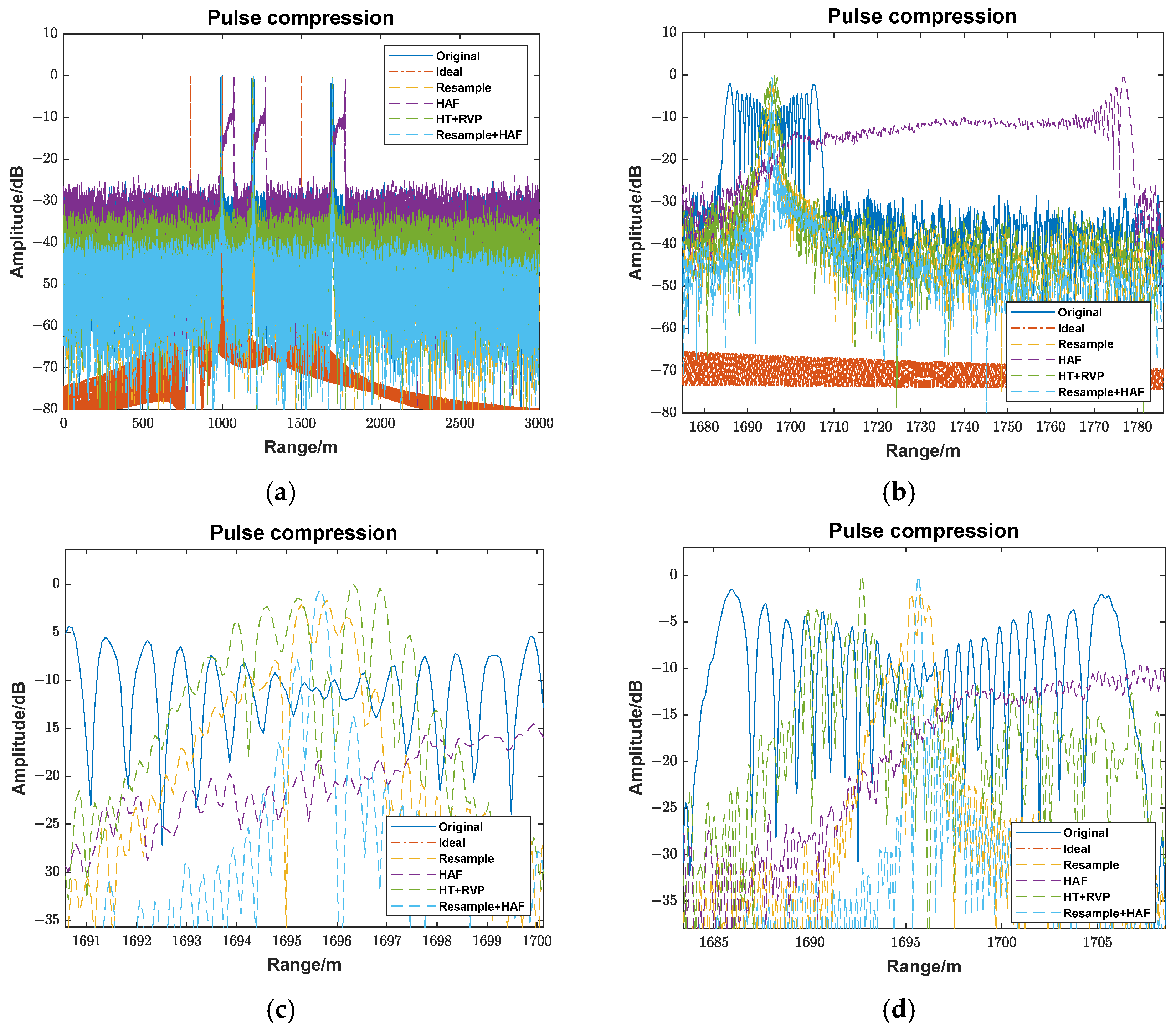MSST is then employed to extract a nonlinear phase for each frequency modulation direction [33], and the transmitted nonlinearity is estimated by two-step integration. Under specific constraints, appropriate extrapolation is applied to estimate the transmitted nonlinearity over the whole symmetrical triangular modulation period. An ideal signal with transmitted nonlinearity is constructed at a higher sampling rate, with a delay time longer than the ranging distance. This signal is mixed with the Doppler frequency from the estimation to create an internal calibration signal. The internal calibration signal is used to resample the actual signal at an equal-phase interval. Subsequently, the high-order ambiguity function (HAF) [24] method is applied to remove the non-constant-speed vibration and residual nonlinear phase. Finally, the compensated positive and negative dechirp signals are used to remove the Doppler frequency caused by constant speed, and the target distance is accurately obtained. The effectiveness of the proposed method is demonstrated through simulation and airborne FMCW Ladar three-dimensional imaging data. The conclusions are summarized.

The rest of this paper is structured as follows. In Section 2, we introduce the signal acquisition method and derive the coupling equation of vibration and frequency modulation nonlinearity, the basic principles and characteristics of MSST, equal-phase interval resampling, HAF, and form the algorithm flow. In Section 3, we use a simulation to verify the effectiveness of the proposed method and compare it with the simple equal-phase interval resampling and HAF methods to highlight its superiority, and we also apply it to actual data for verification. Finally, the conclusion is drawn in Section 4.

2. Method and Theory

2.1. The Process of Obtaining an Ideal Signal

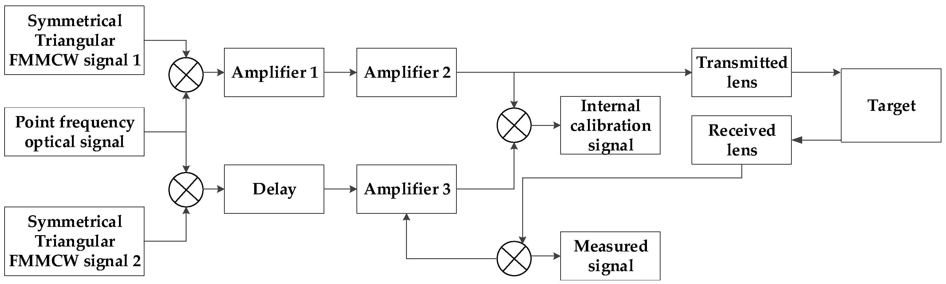
Due to the long working range of the FMCW Ladar system, the echo delay time typically exceeds the signal period. Unlike general systems, where the reference signal is a delayed version of the transmitted signal, both the echo and reference signals are mixed with the transmitted signal. From Figure 1, we use two identical modulations to generate the transmitted and reference signals, respectively. The delay method uses a digital delay to allow for a flexible adjustment based on the working distance. To ensure the target dechirp signal frequency remains within the system’s sampling rate, the echo signal is mixed with the reference signal to form the measurement signal, while the transmitted signal is mixed with the reference signal to create the internal calibration signal.

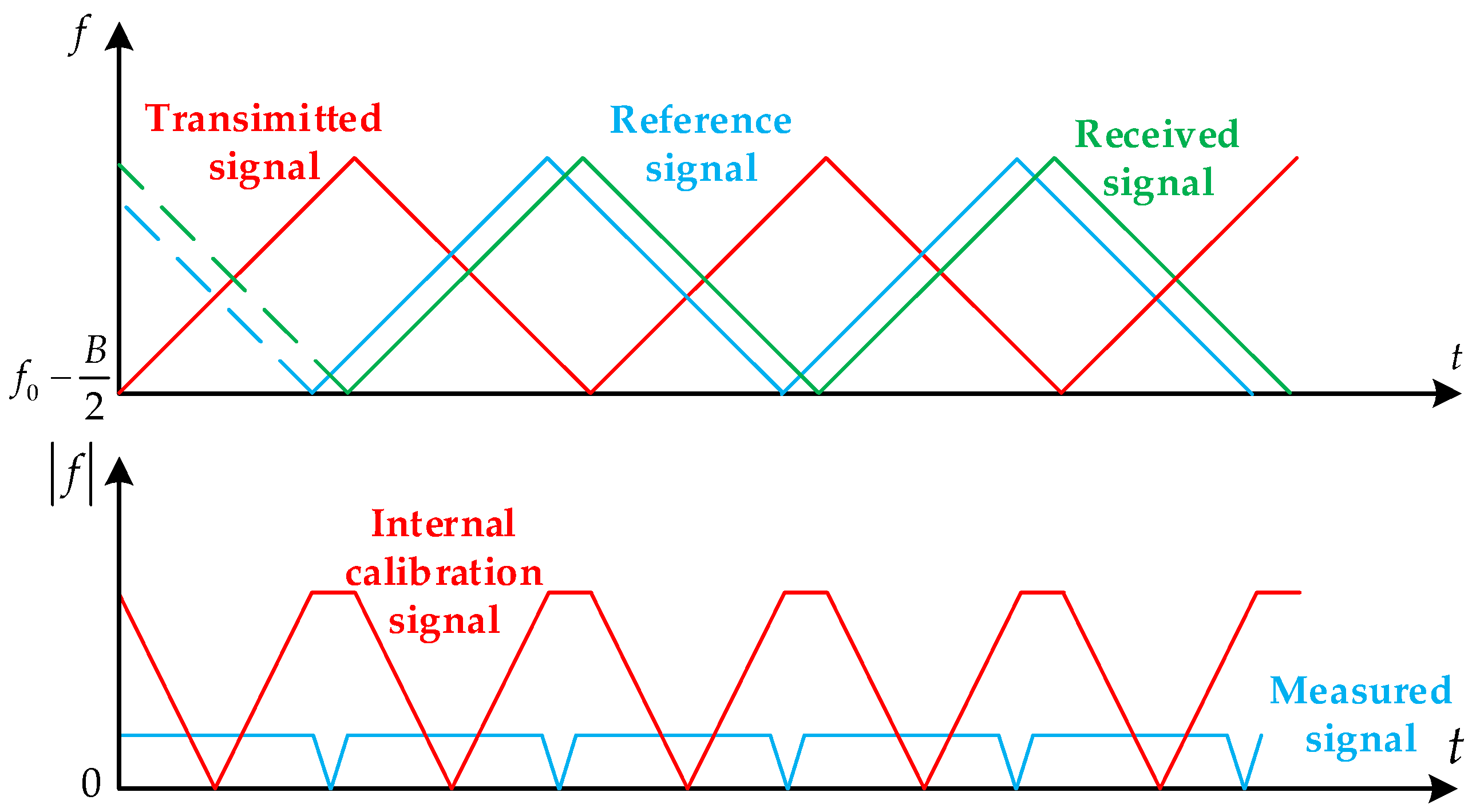
The Ladar transmits a symmetrical triangular FMCW signal, which is modulated into an optical signal and split into two channels. One channel is mixed with the reference signal and sampled as an internal calibration signal. The other channel is reflected by the target, collected by the receiving lens, and mixed with the reference signal as a measurement signal. Figure 2 shows a schematic diagram of the frequency mixing.

The ideal symmetrical triangular FMCW transmitted signal is (ignoring the amplitude representation) as follows:

$$\left\{\begin{array}{l}{s}_{tup}\left(t\right)=exp\left(j2\pi \left(\left(f_c-B/2\right)t+0.5K{t}^2\right)\right)\begin{array}{ll}& 0<t\le T/2\end{array}\\ s_{tdown}\left(t\right)=exp\left(j2\pi \left(\left(f_c+B/2\right)t-0.5K{t}^2\right)\right)\begin{array}{ll}& T/2<t\le T\end{array}\end{array}\right.$$

(1)

where $s_{tup}\left(t\right)$ and $s_{tdown}\left(t\right)$ correspond to the positive and negative frequency modulation of the transmitted signal, respectively, $f_c$ is the carrier frequency, B is the bandwidth, K is the modulation frequency rate, and T is the signal period.

The echo signal with target distance R and the reference signal with reference distance $R_{ref}$ can be derived from the transmitted signal (only the positive frequency modulation part is shown here. The derivation process of the negative portion is the same):

$$\left\{\begin{array}{l}{s}_{rup}\left(t\right)=\exp \left(j2\pi \left(\left(f_c-B/2\right)\left(t-2R/c\right)+0.5K{\left(t-2R/c\right)}^2\right)\right)\\ s_{refup}\left(t\right)=\exp \left(j2\pi \left(\left(f_c-B/2\right)\left(t-2R_{ref}/c\right)-0.5K{\left(t-2R_{ref}/c\right)}^2\right)\right)\end{array}\right.$$

(2)

where $s_{rup}\left(t\right)$ represents the target echo with distance R of the positive received part, $s_{refup}\left(t\right)$ represents the reference signal with delayed distance $R_{ref}$ of the positive received part, and c is the speed of light.

Therefore, the internal calibration signal and measurement signal can be expressed as follows:

$$\left\{\begin{array}{ll}{s}_{dup}\left(t\right)& =s_{refup}^{\ast }\left(t\right)s_{rup}\left(t\right)\\ & =\exp \left(j2\pi \left(\begin{array}{l}\left(f_c-B/2\right)2\left(R-R_{ref}\right)/c\\ +Kt2\left(R-R_{ref}\right)/c+0.5K{\left(2\left(R-R_{ref}\right)/c\right)}^2\end{array}\right)\right)\\ s_{inup}\left(t\right)& =s_{tup}\left(t\right)s_{refup}^{\ast }\left(t\right)\\ & =\exp \left(j2\pi \left(\left(f_c-B/2\right)2R_{ref}/c+Kt2R_{ref}/c-0.5K{\left(2R_{ref}/c\right)}^2\right)\right)\end{array}\right.$$

(3)

where $s_{dup}\left(t\right)$ represents the measurement signal, $s_{inup}\left(t\right)$ represents the internal calibration signal, and * represents the conjugate. At this point, analyzing the frequency of the measurement signal and internal calibration signal, that is, the first-order term in the expression with respect to time, can be derived as follows:

$$\left\{\begin{array}{l}{f}_{dup}=2K\left(R-R_{ref}\right)/c\\ f_{inup}=2K{R}_{ref}/c\end{array}\right.$$

(4)

where $f_{dup}$ represents the frequency of the positive dechirp part in the measurement signal, and $f_{inup}$ represents the frequency of the positive dechirp part in the internal calibration signal. According to the above equation, the target distance can be calculated as follows:

$$R=c{f}_{dup}/2K+R_{ref}$$

(5)

At this point, the target distance can be calculated using only the positive dechirp signal. The above analysis assumes a static target and linear frequency modulation.

2.2. The Impact of Vibration Coupled with Nonlinearity in FMCW Ladar Ranging

The radar signal will be subjected to nonlinearity when it is linearly modulated and transmits through the electrical device. This introduces a nonlinear phase term in the transmitted signal compared to the ideal signal, as follows:

$$s_{teup}\left(t\right)=\exp \left(j2\pi \left(\left(f_c-B/2\right)t+0.5K{t}^2\right)+je\left(t\right)\right)$$

(6)

where $s_{teup}\left(t\right)$ represents the transmitted signal with the nonlinear phase, and $e\left(t\right)$ represents the nonlinear phase. The echo signal and the reference signal will also contain a time-delay term of the nonlinear phase:

$$\left\{\begin{array}{l}{s}_{reup}\left(t\right)=\exp \left(j2\pi \left(\left(f_c-B/2\right)\left(t-\tau \right)+0.5K{\left(t-\tau \right)}^2\right)+je\left(t-\tau \right)\right)\\ s_{refeup}\left(t\right)=\exp \left(j2\pi \left(\left(f_c-B/2\right)\left(t-{\tau }_{ref}\right)-0.5K{\left(t-{\tau }_{ref}\right)}^2\right)+je\left(t-{\tau }_{ref}\right)\right)\end{array}\right.$$

(7)

where $s_{reup}\left(t\right)$ represents the echo signal with nonlinear phase, $s_{refeup}\left(t\right)$ represents the reference signal with the nonlinear phase, and $\tau =2R/c$ and ${\tau }_{ref}=2R_{ref}/c$ are the time delays of the echo signal and reference signal, respectively. It can be derived that the influence of nonlinearity on the measurement signal and internal calibration signal is as follows:

$$\left\{\begin{array}{l}{s}_{deup}\left(t\right)=\exp \left(\begin{array}{l}j2\pi \left(\left(f_c-B/2\right)\left(\tau -{\tau }_{ref}\right)+Kt\left(\tau -{\tau }_{ref}\right)+0.5K{\left(\tau -{\tau }_{ref}\right)}^2\right)\\ +j\left(e\left(t-\tau \right)-e\left(t-{\tau }_{ref}\right)\right)\end{array}\right)\\ s_{ineup}\left(t\right)=\exp \left(\begin{array}{l}j2\pi \left(\left(f_c-B/2\right){\tau }_{ref}+Kt{\tau }_{ref}-0.5K{\tau }_{ref}^2\right)\\ +j\left(e\left(t\right)-e\left(t-{\tau }_{ref}\right)\right)\end{array}\right)\end{array}\right.$$

(8)

where $e\left(t-\tau \right)-e\left(t-{\tau }_{ref}\right)$ represents a nonlinear term in the measured signal, which contains quadratic or higher-order components. Due to these terms, the frequency of the measured signal is no longer a constant, but a time-varying value. This results in main-lobe widening, side-lobe elevation, and potential inaccuracies in measured values after pulse compression.

The above analysis focuses on the effect of nonlinear phase on the signal. However, in practice, vibration is always present. Since Ladar works in the laser band with a short wavelength, even a small movement introduces a large Doppler frequency. In the previous analysis, R is considered as a constant. Under vibration conditions, R is a time-varying value $R\left(t\right)$, and $\tau$ also becomes a time-varying value $\tau \left(t\right)$. At this point, the time-varying distance of the target can be expressed as follows:

$$R\left(t\right)=R_0+{\displaystyle {\int }^{t}v\left(s\right)}ds$$

(9)

where $R_0$ is the initial distance between the target and Ladar at the beginning of the period, $v\left(t\right)$ is the vibration speed, which is also a time-varying value, and $ds$ is the time differential. The time delay $\tau \left(t\right)$ caused by distance is considered into Equation (8), ${\tau }_{ref}$ is still a constant, and then $s_{deup}\left(t\right)$ changes to the following:

$$s_{deup}\left(t\right)=\exp \left(\begin{array}{l}j2\pi \left(\begin{array}{l}\left(f_c-B/2\right)\left(2R\left(t\right)/c-{\tau }_{ref}\right)\\ +Kt\left(2R\left(t\right)/c-{\tau }_{ref}\right)+0.5K{\left(2R\left(t\right)/c-{\tau }_{ref}\right)}^2\end{array}\right)\\ +j\left(e\left(t-2R\left(t\right)/c\right)-e\left(t-{\tau }_{ref}\right)\right)\end{array}\right)$$

(10)

where it can be seen from the change of the nonlinear phase term that the influence of nonlinearity and vibration is coupled with each other. When $R\left(t\right)$ and $e\left(t\right)$ are uniformly modeled with polynomials, the formula below follows:

$$\left\{\begin{array}{l}e\left(t\right)={\displaystyle \sum _{i=2}^k{b}_i{t}^i}\\ R\left(t\right)=R_0+v_{0}t+0.5a{t}^2\end{array}\right.$$

(11)

where $b_i$ is the coefficient of each order polynomial of the nonlinear phase, $v_0$ is the initial velocity of the vibration at the beginning of the period, a is the acceleration of the vibration. The acceleration is also a time-varying value, but it can be approximated as a constant, if a short measurement period is considered, that is, the vibration is modeled as a uniformly accelerated motion within a period. At this time, the $s_{deup}\left(t\right)$ expression can be changed to the following:

$$s_{deup}\left(t\right)=\exp \left(\begin{array}{l}j2\pi \left(\begin{array}{l}\left(f_c-B/2\right)\left(2\left(R_0+v_{0}t+0.5a{t}^2\right)/c-{\tau }_{ref}\right)\\ +Kt\left(2\left(R_0+v_{0}t+0.5a{t}^2\right)/c-{\tau }_{ref}\right)\\ +0.5K{\left(2\left(R_0+v_{0}t+0.5a{t}^2\right)/c-{\tau }_{ref}\right)}^2\end{array}\right)\\ +j\left({\displaystyle \sum _{i=2}^k{b}_i{\left(t-2\left(R_0+v_{0}t+0.5a{t}^2\right)/c\right)}^i}-{\displaystyle \sum _{i=2}^k{b}_i{\left(t-{\tau }_{ref}\right)}^i}\right)\end{array}\right)$$

(12)

The frequency of $s_{deup}\left(t\right)$ is expressed as follows:

$$\begin{array}{ll}{f}_{deup}\left(t\right)& =\left(\left(f_c-B/2\right)2v_0/c+K2R_0/c-K{\tau }_{ref}+K4R_0{v}_0/c^2-K{\tau }_{ref}2v_0/c\right)\\ & +\left(\left(f_c-B/2\right)2a/c+4K{v}_0/c+K4R_{0}a/c^2+K4v_0^2/c^2-K{\tau }_{ref}2a/c\right)t\\ & +\left(3Ka/2c+K4v_{0}a/c^2+K2v_{0}a/c^2\right)t^2+K2a^2{t}^3/c^2\\ & +\left({\displaystyle \sum _{i=2}^k\begin{array}{l}i{b}_i{\left(t-2\left(R_0+v_{0}t+0.5a{t}^2\right)/c\right)}^{i-1}\left(1-2\left(v_0+at\right)/c\right)\\ -{\displaystyle \sum _{i=2}^{k}i{b}_i{\left(t-{\tau }_{ref}\right)}^{i-1}}\end{array}}\right)/2\pi \end{array}$$

(13)

From Equation (4), the ideal dechirp frequency should be point frequency. However, when considering both vibration and nonlinearity, the frequency includes a constant term, a Doppler frequency term, a term related to the initial distance and velocity, and higher-order phase components. This results in a highly complex expression. Under polynomial modeling, the effects of vibration and nonlinearity become coupled, doubling the order of the polynomial expression. Due to the limited sampling frequency resolution of FMCW Ladar, the expression can be simplified for analysis. By ignoring the $c^2$ term in the denominator of each order polynomial coefficient, the simplified frequency expression becomes the following:

$$\begin{array}{ll}{f}_{deup}\left(t\right)& \approx \left(\left(f_c-B/2\right)2v_0/c+K2R_0/c-K{\tau }_{ref}\right)\\ & +\left(\left(f_c-B/2\right)2a/c+4K{v}_0/c\right)t+3Ka{t}^2/2c\\ & +\left({\displaystyle \sum _{i=2}^4\begin{array}{l}i{b}_i{\left(t-2\left(R_0+v_{0}t+0.5a{t}^2\right)/c\right)}^{i-1}\left(1-2\left(v_0+at\right)/c\right)\\ -{\displaystyle \sum _{i=2}^{4}i{b}_i{\left(t-{\tau }_{ref}\right)}^{i-1}}\end{array}}\right)/2\pi \end{array}$$

(14)

where the phase of the nonlinearity and vibration coupled part only discards the terms higher than the third-order t, though it is not fully expanded. From Equation (14), it is evident that the expression still includes terms ranging from constants to higher-order terms of t. Analyzing the frequency expression, the constant terms consist of the Doppler frequency and the initial range difference. The coupled part also contains terms such as $-2b_2\left(2R_0/c\right)+4b_2{\tau }_{ref}$, which causes the frequency shift and the approximate nonlinear phase when only a stationary target is considered. Among the first-order terms, since the denominator contains more c and is multiplied by a smaller t, this makes their contribution smaller than the constant term. Similarly, the higher order terms have even less impact. These terms primarily affect the peak shape and increase the side lobes.

2.3. Multiple Synchro-Squeezing Transform

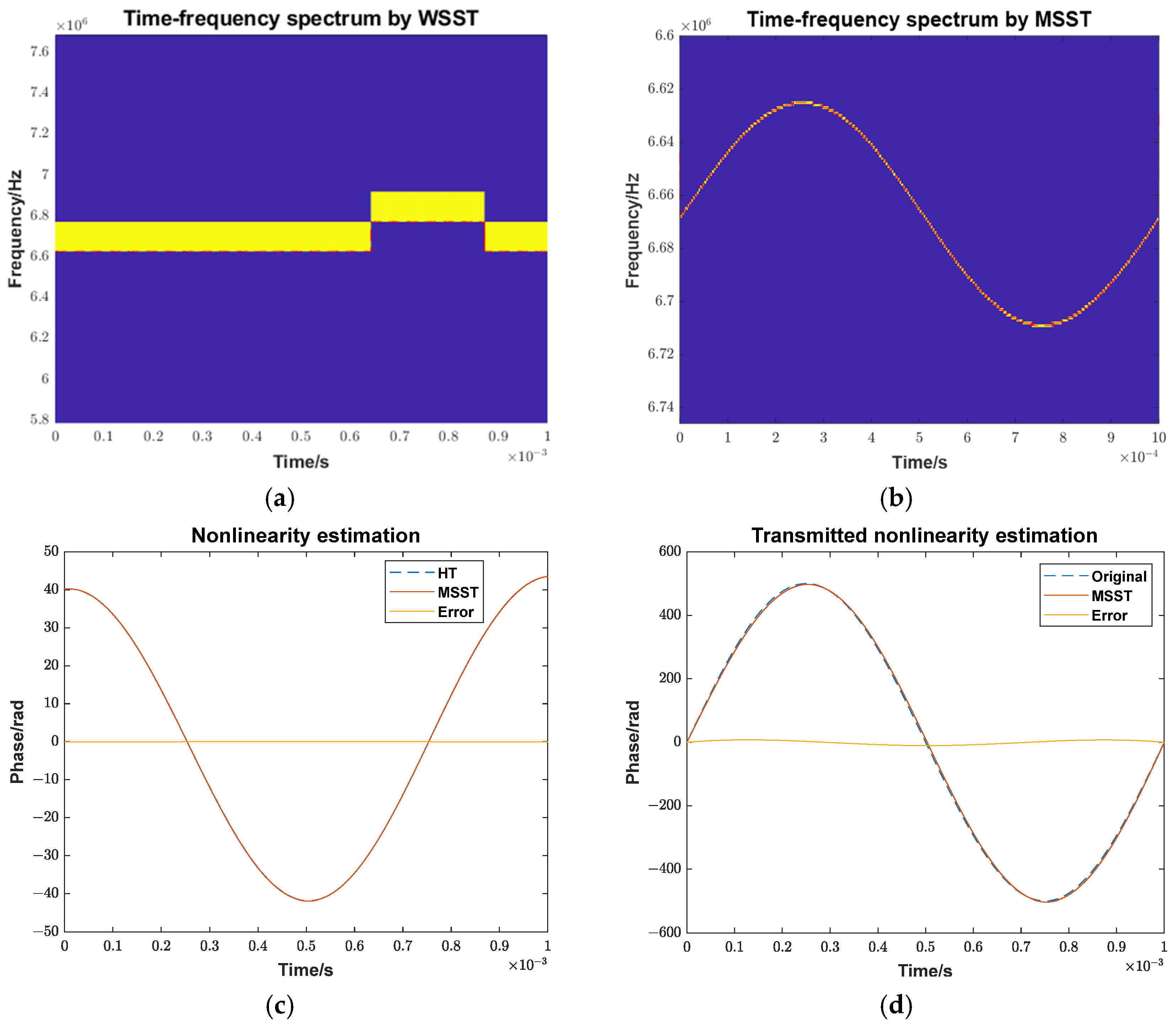
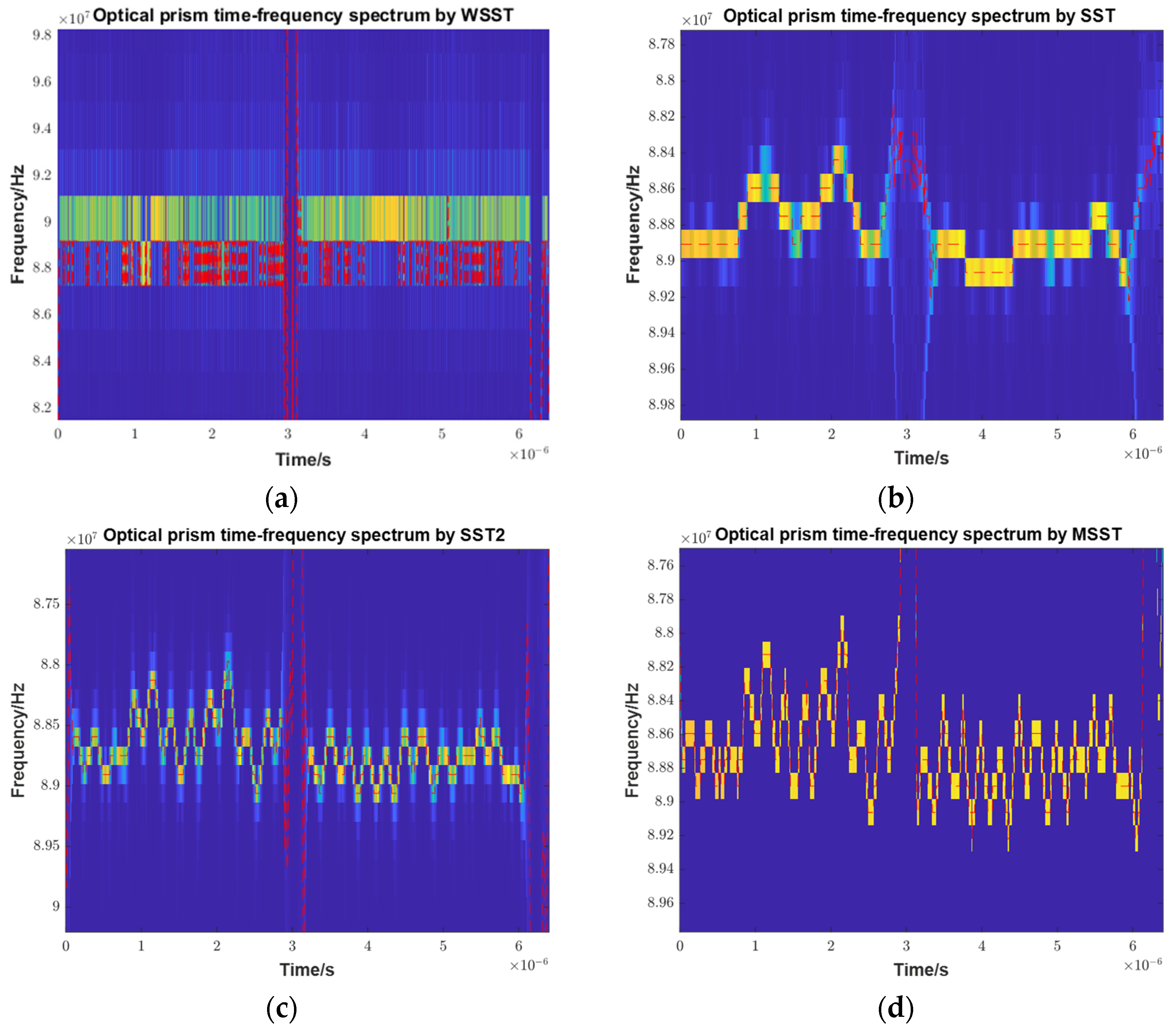
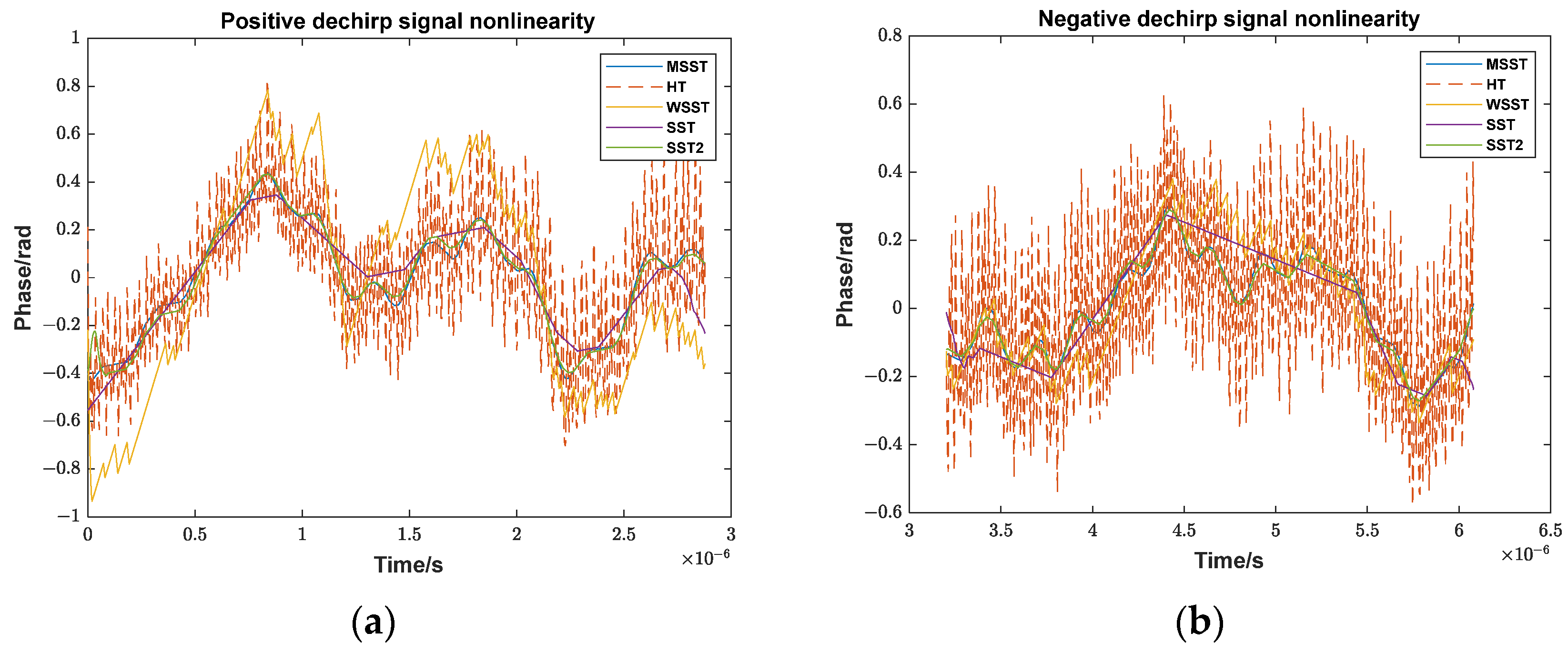
To compensate for frequency modulation nonlinearity, the nonlinear phase of the internal calibration signal must be analyzed, because it does not contain the phase change caused by vibration. However, due to the inevitable presence of phase noise in the actual signals, the nonlinear phase extracted directly via HT is not smooth and is unsuitable for constructing a reference signal. This paper proposes to use MSST, which is an improvement of synchrosqueezing transform (SST). SST improves time–frequency resolution over the short-time Fourier transform (STFT) by rearranging the signal energy in the time–frequency domain [34]. MSST performs SST iteratively to achieve a better energy concentration. Compared with the second-order SST and higher-order SST, MSST requires only a single STFT computation, offering a lower computational cost while ensuring accurate signal reconstruction.

MSST operates within the STFT framework. Firstly, the STFT of the full-period optical prism signal is expressed as follows:

$$G_{deup}\left(t,\omega \right)={\displaystyle {\int }_{-\infty }^{+\infty }g\left(u-t\right)s_{deup}\left(u\right)e^{-i\omega \left(u-t\right)}}du$$

(15)

where $G_{deup}\left(t,\omega \right)$ represents the transformed time–frequency matrix, $g\left(t\right)$ represents the compact support window, and $\omega$ is the angular frequency. The phase of $s_{deup}\left(t\right)$ can be expressed by Equation (14) as follows:

$$\phi \left(t\right)=2\pi {\displaystyle \int f_{deup}\left(t\right)dt}$$

(16)

Equation (15) can be derived as follows:

$$G_{deup}\left(t,\omega \right)=s_{deup}\left(t\right)F\left(g\left(\omega -{\phi }^{\prime }\left(t\right)\right)\right)$$

(17)

where $F\left(·\right)$ represents Fourier transform. We can calculate the partial derivative of Equation (17) with respect to t:

$${\partial }_t{G}_{deup}\left(t,\omega \right)={\partial }_t\left(s_{deup}\left(t\right)F\left(g\left(\omega -{\phi }^{\prime }\left(t\right)\right)\right)\right)=G_{deup}\left(t,\omega \right)i{\phi }^{\prime }\left(t\right)$$

(18)

The estimation of the instantaneous angular frequency can be derived as follows:

$$\widehat{{\phi }^{\prime }}\left(t\right)=\widehat{\omega }\left(t,\omega \right)=\mathrm{Re}\left[{\displaystyle \frac{{\partial }_t{G}_{deup}\left(t,\omega \right)}{i{G}_{deup}\left(t,\omega \right)}}\right]$$

(19)

For weakly time-varying signals, this estimation provides a good approximation of the signal’s intermediate frequency. SST employs a frequency rearrangement operator to converge the extended time–frequency coefficients, expressed as follows:

$$Ts\left(t,\eta \right)={\displaystyle {\int }_{-\infty }^{+\infty }{G}_{deup}\left(t,\omega \right)\delta \left(\eta -\widehat{\omega }\left(t,\omega \right)\right)}d\omega$$

(20)

Through SST, the energy of the time–frequency matrix is concentrated around the estimated intermediate frequency. MSST extends this process by iteratively repeating the synchronous compression step, achieving further refinement, as follows:

$$\begin{array}{ll}T{s}_2\left(t,\eta \right)& ={\displaystyle {\int }_{-\infty }^{+\infty }Ts\left(t,\xi \right)\delta \left(\eta -\widehat{\omega }\left(t,\xi \right)\right)}d\xi \\ & ={\displaystyle {\int }_{-\infty }^{+\infty }{\displaystyle {\int }_{-\infty }^{+\infty }{G}_{deup}\left(t,\omega \right)\delta \left(\xi -\widehat{\omega }\left(t,\omega \right)\right)d\omega }}\delta \left(\eta -\widehat{\omega }\left(t,\xi \right)\right)d\xi \\ & ={\displaystyle {\int }_{-\infty }^{+\infty }{G}_{deup}\left(t,\omega \right)}{\displaystyle {\int }_{-\infty }^{+\infty }\delta \left(\xi -\widehat{\omega }\left(t,\omega \right)\right)\delta \left(\eta -\widehat{\omega }\left(t,\xi \right)\right)d\xi d\omega }\\ & ={\displaystyle {\int }_{-\infty }^{+\infty }{G}_{deup}\left(t,\omega \right)\delta \left(\eta -\widehat{\omega }\left(t,\widehat{\omega }\left(t,\omega \right)\right)\right)}d\omega \end{array}$$

(21)

Performing SST again on the basis of SST is equivalent to a new estimation of frequency to redistribute the energy of STFT. Thus, the core improvement of MSST over SST lies in its multiple frequency estimates.

Here, the previous phase Equation (16) is expanded using Taylor series:

$$\phi \left(t\right)=\phi \left(u\right)+{\phi }^{\prime }\left(u\right)\left(t-u\right)+0.5{\phi }^{″}\left(u\right){\left(t-u\right)}^2+O\left({\phi }^{″}\left(u\right)\right)$$

(22)

Inserting this into Equation (15) and defining the Gaussian window function as $g\left(t\right)=e^{-0.5t^2}$, the time–frequency representation after STFT can be derived as follows:

$$G_{deup}\left(t,\omega \right)={\displaystyle {\int }_{-\infty }^{+\infty }{e}^{-0.5{\left(u-t\right)}^2}{e}^{i\phi \left(t\right)}{e}^{-i\omega \left(u-t\right)}}du=e^{i\phi \left(t\right)}{\displaystyle \frac{1}{\sqrt{1-i{\phi }^{″}\left(t\right)}}}{e}^{{\displaystyle \frac{{\left(\omega -{\phi }^{\prime }\left(t\right)\right)}^2}{2\left(1-i{\phi }^{\prime }\left(t\right)\right)}}}$$

(23)

Inserting it into the angular frequency estimation Equation (19), we receive the following formula:

$$\widehat{\omega }\left(t,\omega \right)={\phi }^{\prime }\left(t\right)+{\displaystyle \frac{{\phi }^{″}{\left(t\right)}^2}{1+{\phi }^{″}{\left(t\right)}^2}}\left(\omega -{\phi }^{\prime }\left(t\right)\right)$$

(24)

Then, the frequency after the twice-frequency estimation can be expressed as follows:

$$\widehat{\omega }\left(t,\widehat{\omega }\left(t,\omega \right)\right)={\phi }^{\prime }\left(t\right)+{\displaystyle \frac{{\phi }^{″}{\left(t\right)}^2}{1+{\phi }^{″}{\left(t\right)}^2}}\left(\widehat{\omega }\left(t,\omega \right)-{\phi }^{\prime }\left(t\right)\right)={\phi }^{\prime }\left(t\right)+{\left({\displaystyle \frac{{\phi }^{″}{\left(t\right)}^2}{1+{\phi }^{″}{\left(t\right)}^2}}\right)}^2\left(\omega -{\phi }^{\prime }\left(t\right)\right)$$

(25)

According to the above derivation, the frequency and SST after multiple rearrangements can be expressed as follows:

$$\left\{\begin{array}{l}{\widehat{\omega }}_N\left(t,\omega \right)={\phi }^{\prime }\left(t\right)+{\left({\displaystyle \frac{{\phi }^{″}{\left(t\right)}^2}{1+{\phi }^{″}{\left(t\right)}^2}}\right)}^N\left(\omega -{\phi }^{\prime }\left(t\right)\right)\\ T{s}_N\left(t,\eta \right)={\displaystyle {\int }_{-\infty }^{+\infty }{G}_{deup}\left(t,\omega \right)\delta \left(\eta -{\widehat{\omega }}_N\left(t,\omega \right)\right)}d\omega \end{array}\right.$$

(26)

where N represents the number of rearrangements. Through iterative rearrangements, the frequency estimation continuously converges to the intermediate frequency, resulting in a more concentrated time–frequency energy distribution for the target. The time–frequency curve is extracted by ridge detection more accurately.

2.4. Equal-Phase Interval Resampling

From Equation (3), for ideal linear frequency modulation and a stationary target, the signal phase is a linear function of time. Under equal-time interval sampling, the phase changes uniformly, allowing direct spectrum analysis via FFT. However, when frequency modulation nonlinearity and vibration are modeled as polynomial functions, the signal phase becomes a polynomial function of time. In this case, equal-time interval sampling results in non-uniform phase changes, and direct FFT analysis will introduce problems such as main-lobe widening and side-lobe elevation, which degrades the target peak shape. The signal is transformed from Equations (12) and (14):

$$s_{deup}\left(t\right)=\exp \left(j2\pi \left(\psi +\left(\left(f_c-B/2\right)2v_0/c+K2R_0/c-K{\tau }_{ref}\right){\tau }_0\theta \left(t\right)\right)\right)$$

(27)

where $\psi$ represents constant phases, ${\tau }_0$ represents the delay corresponding to the initial distance, and $\theta \left(t\right)$ is expressed as follows:

$$\theta \left(t\right)=t+{\displaystyle \sum _{i=2}^N\frac{a_i}{\left(\left(f_c-B/2\right)2v_0/c+K2R_0/c-K{\tau }_{ref}\right)}}{t}^i$$

(28)

where $a_i$ represents the corresponding coefficients of each order polynomial. In this case, the phase of the signal is collapsed to $\theta \left(t\right)$ as a function of the independent variable. The Doppler frequency is considered when simplifying the expression of first-order phase coefficient. If the signal is resampled at an equal-phase interval about $\theta \left(t\right)$, instead of equal-time intervals, the influence of high-order terms is eliminated during FFT analysis. This resampling process removes the interference of a polynomial phase, improving peak shape.

2.5. High-Order Ambiguity Function

Since the vibration of the target cannot be completely equivalent to a constant speed, the effect of high-order phase terms may still remain after equal-phase interval resampling. In this case, the signal is expressed as follows:

$$s_{deup}^{re}\left(t\right)=\exp \left(j2\pi \left(m_o+m_{1}t+{\displaystyle \sum _{i=2}^N{m}_i{t}^i}\right)\right)$$

(29)

where $s_{deup}^{re}\left(t\right)$ represents the resampled signal, and $m_i$ represents the coefficient of polynomial phase. By segmenting the signal into equal interval and alternately conjugating and multiplying them, a single-frequency signal can be obtained as follows:

$$HI{M}_N\left[s_{deup}^{re}\left(t\right),{\tau }_{lag}\right]=\exp \left(j2\pi {\tilde{f}}_{N}t\right)$$

(30)

where $HIM\left(·\right)$ represents the ambiguity operator, and ${\tau }_{lag}$ represents the delay of each interval. Equation (30) is the result of the alternating conjugate multiplication of N-order signals, and its frequency is as follows:

$${\tilde{f}}_N=N!{\tau }_{lag}^{N-1}{m}_N$$

(31)

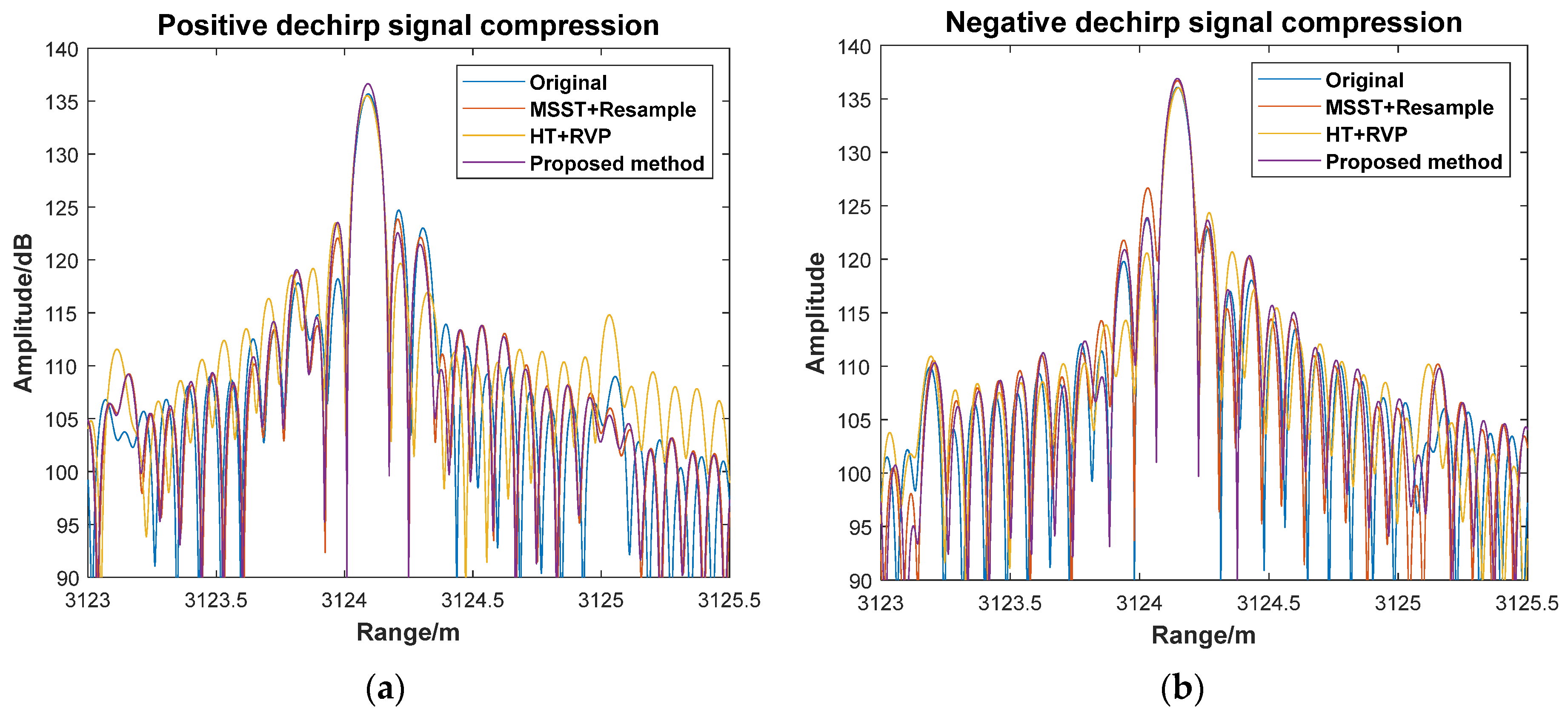
The frequency of the ambiguity function can be analyzed using FFT. Combining with this relationship, high-order polynomial terms can be compensated step-by-step until only the first-order phase term remains. Subsequently, the symmetrical triangular wave modulation is utilized to compensate for the Doppler frequency caused by constant speed.

Theoretically, the HAF method can directly compensate for both vibration and nonlinearity. However, it suffers from the accumulation of errors in polynomial coefficient estimation and requires a high signal-to-noise ratio. Therefore, the primary compensation method remains equal-phase interval resampling, with the HAF method applied for residual compensation.

2.6. Proposed Method

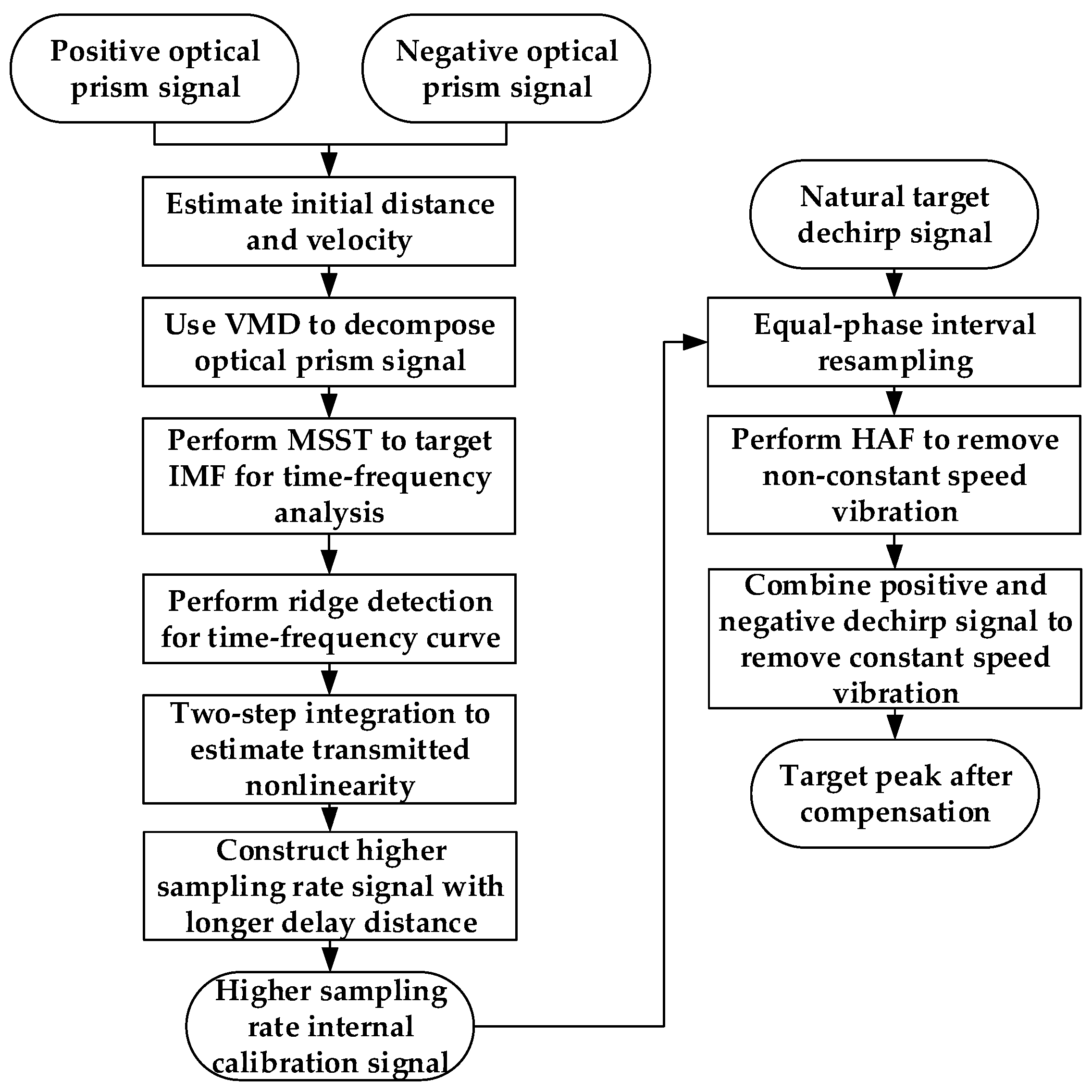
The proposed method for the simultaneous compensation of frequency modulation nonlinearity and vibration is implemented as Figure 3:

(a) Preliminary Estimation: Select the optical prism actual signal, which has a high signal-to-noise ratio, and perform FFT to preliminarily estimate the target distance and constant speed of vibration.

(b) Signal Decomposition: Apply variational mode decomposition (VMD) [35] to the positive and negative dechirp signals to extract the intrinsic mode function (IMF) of the optical prism signal, eliminating noise and harmonics interference.

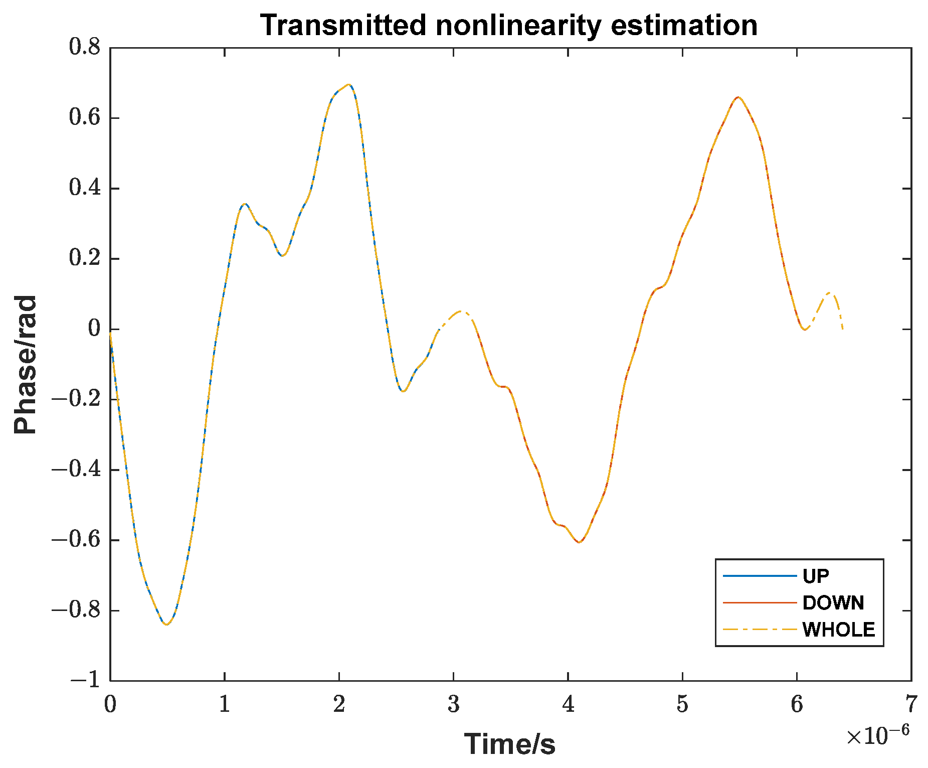
(c) Time–Frequency Analysis: Perform MSST on the optical prism signals’ IMFs and extract the time–frequency variation curve using ridge detection. The ideal frequency is a point frequency, and the Doppler frequency from constant speed is also a point frequency. The remaining variations represent frequency modulation nonlinearity, the non-constant speed term of vibration, and phase noise.

(d) Nonlinear Phase Extraction: Integrate the time–frequency curve and remove the linear trend to obtain the nonlinear phase in the optical prism signal. Estimate the transmitted signal nonlinearity based on first-order Taylor series expansion with preliminary prism distance. The small delay of the optical prism echo relative to the period justifies the use of first-order approximation.

(e) Signal Alignment and Construction: Cyclically shift the transmitted nonlinearity estimation to align with the reference delay signal period. Construct an ideal transmitted signal at a higher sampling rate, adding the estimated nonlinearity. Generate an echo signal with a delay greater than the maximum range of the actual signal, adding nonlinearity corresponding to the delay cycle shift. Mix the two signals and add the Doppler frequency from the estimated speed.

(f) Resampling: Taking the constructed internal calibration signal as a reference, interpolate the time points corresponding to its equal-phase points, and resample the actual signal at these time points.

(g) Residual Compensation: Apply the HAF method to compensate for residual polynomial phase errors. Average the positive and negative frequency modulation peaks to remove the Doppler frequency influence caused by the constant speed.

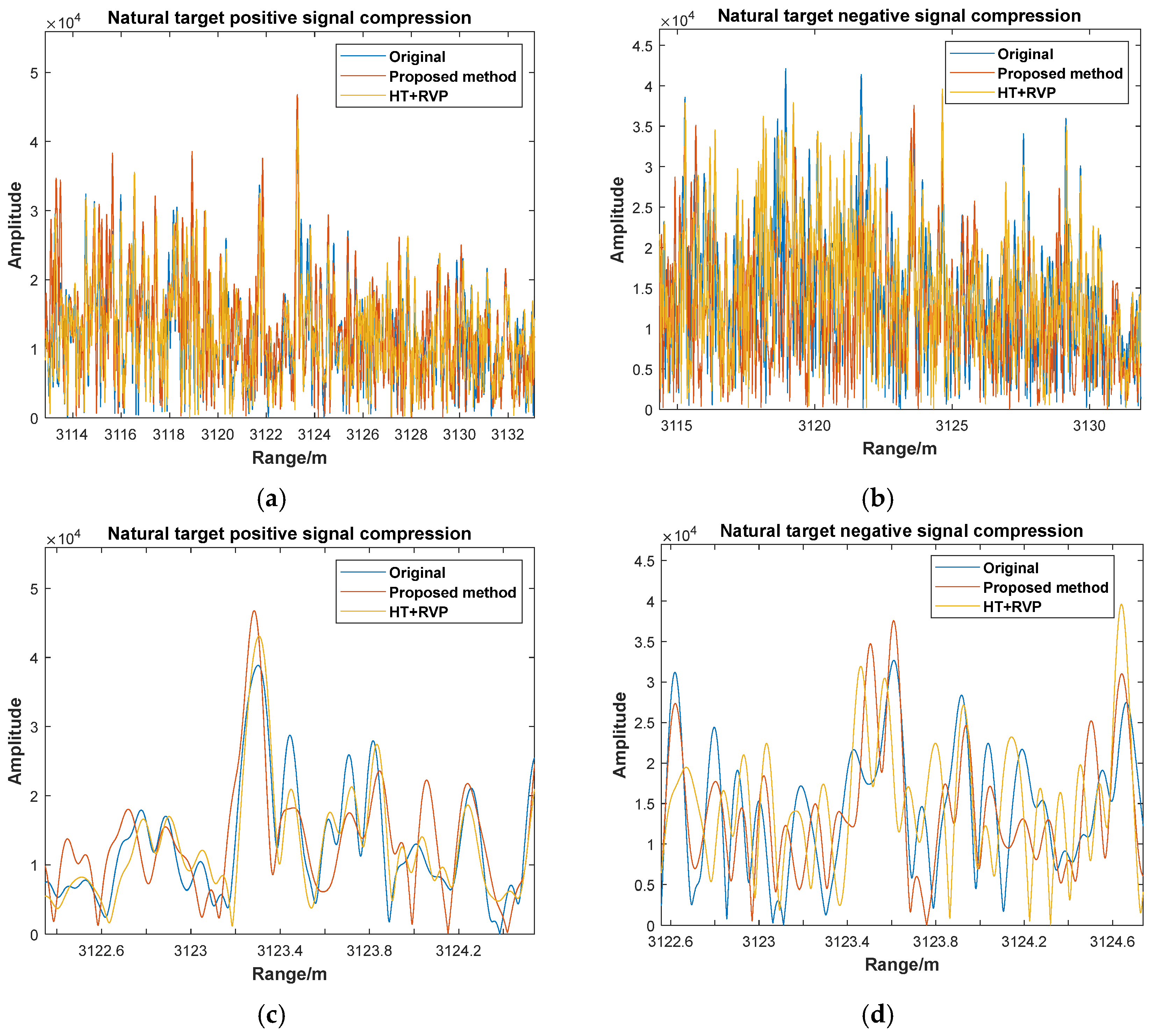
3. Experimental Analysis

3.1. Simulation Analysis

To verify the effectiveness of the proposed method combining MSST, equal-phase interval resampling, and HAF, a sawtooth wave signal is used and the frequency modulation nonlinearity and vibration are added. After compensation, the target peak value still has an offset caused by the constant speed compared to the ideal situation.

The simulation parameters include a period of 1 ms, a bandwidth of 500 MHz, and a sampling frequency of 20 MHz. Three targets are set at 800 m, 1000 m, and 1500 m, and the reference signal is delayed by 2000 m. A longer period is chosen to extend the detection range and emphasize the impact of vibration, which becomes more pronounced over extended durations and smaller frequency modulation rates. Vibration is modeled as a constant acceleration, with an initial velocity of 0.5 m/s and an acceleration of 10 m/s². Frequency modulation nonlinearity is introduced in sinusoidal form to simulate the nonlinear phase effect of high-order polynomials.

From Figure 4a,b, it can be seen that the MSST time–frequency analysis achieves a high time–frequency resolution, accurately depicting the variations in the time–frequency curve, while WSST cannot achieve that. From Figure 4c,d, it can be seen that the estimated nonlinearity in the internal calibration signal and transmitted signal closely match the original signal’s nonlinearity. Although the estimation error in Figure 4d is slightly larger, it does not significantly impact the subsequent compensation. This is related to the larger reference delay setting, which is also encountered in actual data processing. From Figure 4e–h, it can be seen that the MSST time–frequency analysis still achieves a high time–frequency resolution with 10 dBW Gaussian noise to the reference signal.

From Figure 5a, the actual compressed peak deviates significantly from the ideal peak due to the Doppler frequency effect, as expected. From Figure 5b, the blue line represents the result of direct pulse compression, which is highly distorted by errors, making the target position identification impossible. From Figure 5c, the yellow line shows the result of MSST and equal-phase interval resampling, which improves the peak resolution but exhibits bifurcation due to non-constant vibration effects. Its peak position is offset by 0.15 m and its PSLR is −0.455 dB. The purple line represents the fifth-order HAF compensation result. Although VMD has been used to decompose the single target peak before HAF coefficient estimation, strong interference leads to inaccurate polynomial coefficient estimation and error accumulation, resulting in unsatisfactory compensation. The green line shows the combined result of HT and RVP compensation. Its peak position is offset by 0.67 m and its PSLR is −0.446 dB. The light-blue line shows the combined result of equal-phase interval resampling and HAF compensation. HAF compensates for nonlinearity from fourth-order to second-order, achieving a near-ideal performance. Its PSLR is −7.836 dB. From Figure 5d, when the noise is added to the reference signal, other methods’ effects remain unchanged, the HAF method still compensates incorrectly, and the HT method fails to extract the nonlinear phase, which makes the RVP method fail and its peak position is offset by 2.93 m.

The simulation confirms the feasibility of the proposed method. However, it is also found from the implementation process that HAF requires an independent target and a strong signal-to-noise ratio signal. While VMD can solve the former, the latter depends on the actual signal condition.

3.2. Actual Data Analysis

Use FMCW Ladar airborne three-dimensional imaging data for verification. The signal is modulated by a symmetrical triangular wave, with a period of 6.4 µs, a bandwidth of 2 GHz, and a sampling frequency of 300 MHz. The reference delay is set to 20.7 µs. The initial analysis focuses on the optical prism echo.

From Figure 6, which shows the spectrum of the optical prism signal, it can be seen that the prism signal energy is dominant. However, low-frequency noise and harmonic peaks remain prominent in the spectrum, which will affect the extraction of the nonlinear phase. To solve this, VMD is applied to decompose the signal and extract target IMF.

After decomposition, the IMF containing the target peak can be identified based on the signal spectrum amplitude. As shown in Figure 7, the target is located in IMF2. A time–frequency analysis is performed on the IMF2 using MSST. For comparison, other methods, WSST, SST, and second-order SST, are applied directly to the original signal.

From Figure 8, the time–frequency diagrams reveal that the frequency resolution of WSST (using MATLAB’s function) is limited. The ridge detection result oscillates within two frequency resolution units, failing to accurately capture time–frequency variations. SST shows a better time–frequency resolution. The trend of time–frequency changes can be observed. Both second-order SST and MSST provide a finer time–frequency resolution, and the result of MSST is more concentrated than second-order SST2. The nonlinear phase is estimated by integrating the time–frequency curve and removing the linear trend.

From Figure 9, the red dotted line represents the nonlinear phase estimated using HT to directly extract the phase and remove the linear trend. However, due to phase noise and other peaks in the spectrum, the extracted nonlinear phase exhibits many burrs and abrupt changes. Its nonlinear phase trend is difficult to fit directly with the polynomial phase or sinusoidal form. In contrast, the blue solid line shows the nonlinear phase estimated by integrating the time–frequency curve extracted from IMF2 using MSST time–frequency analysis and ridge detection. This approach yields a smoother phase trend, removing the remaining noise on the phase, which is more suitable for compensation operation. The orange line represents the nonlinear phase estimated by the WSST method. Due to its poor time–frequency analysis, the estimated nonlinear phase is different from that estimated by the HT method. The purple line shows the estimation by the SST method, and due to its time–frequency resolution being low, the trend of the estimated nonlinear phase is similar to that of the HT method, but the details are missing, especially in the negative dechirp part. The green line represents the estimation by the second-order SST method, which has a high time–frequency resolution and the estimated nonlinear phase is close to the result of MSST.

Due to the difficulty of polynomial fitting, the nonlinear phases of the positive and negative dechirp signals are arranged, with constraints ensuring phase continuity at the period’s start and end. From Figure 10, based on the first-order Taylor series expansion and the fact that the optical prism echo delay is much smaller than the reference delay and period, the transmitted nonlinearity for the whole period is extrapolated and estimated.

Since digital methods are used to construct complex reference signals, and the reference delay distance must exceed the actual maximum detection range according to the Nyquist theorem, the sampling rate of the constructed signal should be greater than the actual signal sampling rate. An ideal transmitted signal with a sampling rate of 600 MHz is constructed. The transmitted nonlinearity is cyclically shifted according to the optical prism delay and added to the signal. Similarly, a reference signal with a delay distance greater than the actual signal detection range is constructed. The transmitted nonlinearity is cyclically shifted according to the reference distance and added to the reference signal. These signals are then mixed to create an internal calibration signal for equal-phase interval resampling, with the Doppler frequency phase corresponding to the estimated constant velocity added. As the constructed internal calibration signal does not contain random phase noise, HT is used to directly extract its phase. The equal-phase axis is determined according to phase expansion range. The corresponding sampling time points are interpolated for each phase point. The actual signal is then resampled according to this non-uniformly spaced time axis.

$$R_r^1=F_S/2·c/\left(2K{R}_{ref}^0\right)·N_F·R_r^0$$

(32)

where $R_r^1$ is the distance axis after resampling, $R_r^0$ is the original distance axis, $F_s$ is the original sampling frequency, $R_{ref}^0$ is the set reference delay, and $N_F$ is the up-sampling multiple. This equation is derived with π as the sampling interval. If the sampling interval is reduced, it must be multiplied by the corresponding factor. An additional explanation for constructing the reference signal is provided. In addition to ensuring the distance satisfies the Nyquist sampling theorem, the system’s internal calibration signal contains phase noise. Furthermore, due to the delay uncertainty caused by working distance, it is difficult to use first-order Taylor series expansion to approximate the small delay required for transmitted nonlinearity estimation. Another reason is that, due to hardware limitations, the transmitted signal is emitted later than the reference signal, resulting in a negative delay for the reference signal under zero internal delay. Since the internal calibration signal’s sampling rate is only 50 MHz, lower than that of the measurement signal, there is aliasing even under zero delay, preventing accurate internal delay calibration. Constructing a digital signal effectively avoids these issues.

After compensation, the pulse compression result of the optical prism signal is compared with the original signal’s direct pulse-pressure compression result in Figure 11.

As shown in Figure 11, the blue line shows FFT for the original signal. The red line represents the result of equal-phase interval resampling using the constructed internal calibration signal described above. For both positive and negative beat frequencies, the prism peak is slightly stronger after compensation. From

Table 1. A comparison of indexes after pulse pressure.

	Original		MSST + Resample		HT + RVP		Proposed Method
	P	N	P	N	P	N	P	N
Bandwidth/m	0.0749	0.0740	0.0728	0.0725	0.0980	0.0946	0.0728	0.0723
PSLR/dB	−10.97	−12.36	−12.87	−10.29	−12.00	−11.68	−13.12	−13.01
ISLR/dB	−8.93	−9.64	−9.89	−8.37	−9.40	−9.74	−9.97	−9.59

, the side lobe of the positive dechirp signal is suppressed 1.9 dB, while the side lobe of the negative dechirp signal is elevated 2.07 dB. The yellow line indicates the compensation results of the HT combined with the RVP method. The side lobe of the positive dechirp signal is suppressed 1.03 dB, while the side lobe of the negative dechirp signal is elevated 0.68 dB. The main lobe is widened about 0.022 m. The purple line represents the compensation result of the proposed method. The side lobe of the positive dechirp signal is suppressed 2.15 dB, while the side lobe of the negative dechirp signal is suppressed 0.65 dB. From the direct pulse-pressure results, the side lobe is already very low near the main-lobe intersection, which means that the frequency modulation nonlinearity and non-constant-speed vibration do not seriously distort the peak shape. Nevertheless, the proposed method still provides meaningful compensation.

To further validate the method, it is applied to natural-target echoes to assess its effectiveness in removing nonlinearity and vibration.

Due to the weak energy of the natural-target echo, HAF compensation is omitted after resampling. As shown in Figure 12c,d, the amplitude of the natural target after the proposed method’s compensation is slightly higher than that of before, and nearby maximum points are suppressed. From Figure 12b, it is evident that some extreme points with amplitudes higher than the target peak at a closer distance are suppressed. However, HT combined with the RVP method has a poor effect on the suppression of noise peaks in this case, and cannot make the target peak prominent. The proposed method enhancement of the target peak energy and the suppression of noise demonstrates the effectiveness of the method in removing nonlinearity and non-constant-speed vibration, facilitating peak extraction.

4. Discussion

Here, we discuss the reasons for designing the internal calibration path in the actual system while not utilizing its data. As previously mentioned, the low sampling rate and uncalibrated internal delay make the data inconvenient to use. Furthermore, the reference signal delay of 20.7 µs designed according to the actual working distance is equivalent to three times the signal period (6.4 µs) plus 1.5 µs, which is too large to estimate transmitted nonlinearity. However, it has been verified that the nonlinearity remains consistent across each period under zero-delay conditions, which is a prerequisite for analysis. Under these conditions, the proposed method is applied, and the target signal is compensated based on the actual internal calibration signal.

Firstly, from Figure 13, the effect of the MSST time–frequency analysis for estimating nonlinearity remains applicable. However, unlike the optical prism nonlinearity discussed earlier, the results here show no similarity.

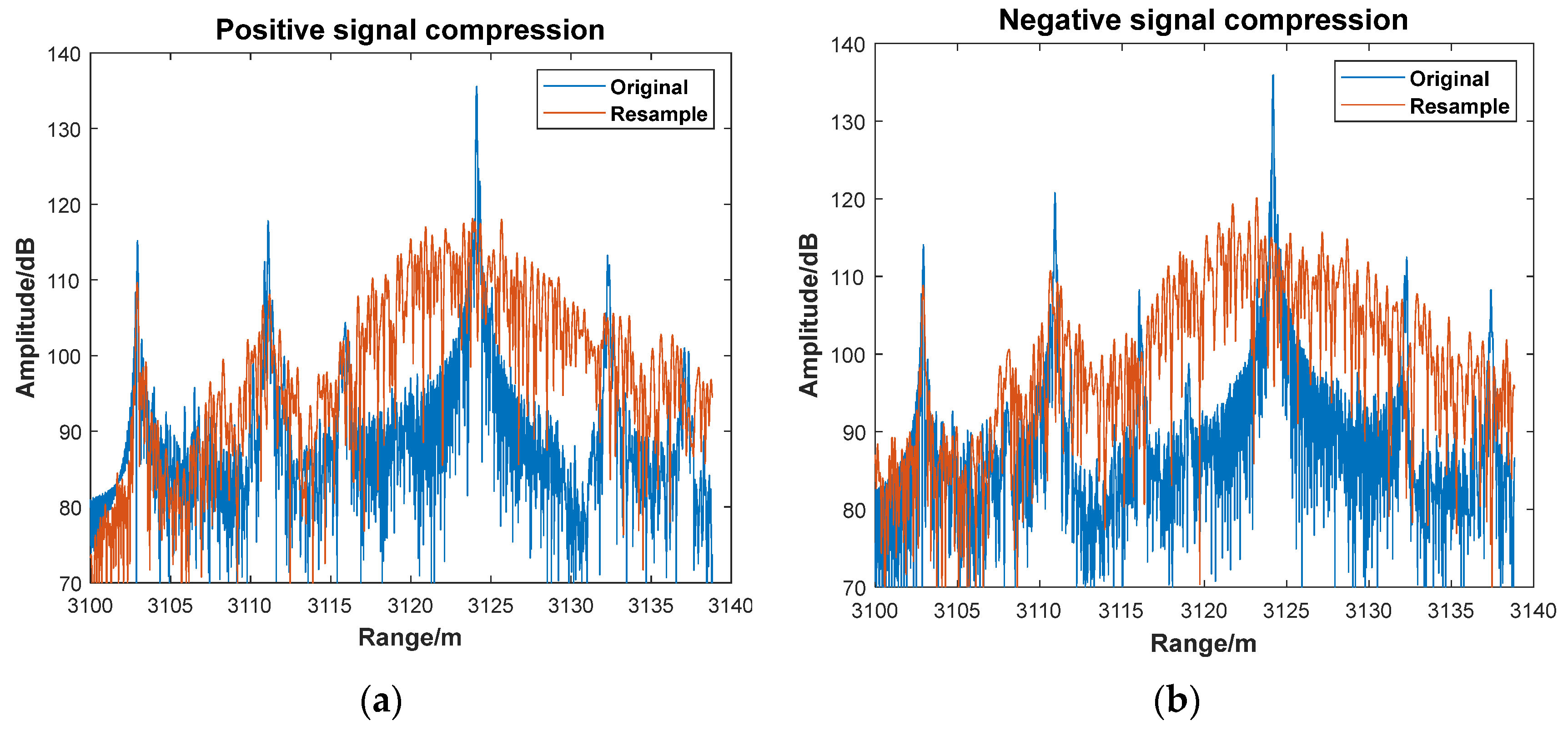
Next, the internal calibration signal is directly used for resampling tests. Due to the limited number of points in the internal calibration signal, the phase curve obtained by integrating the time–frequency curve has a small range. If the phase interval $\pi$ is used as the equal-phase interval, the resulting signal contains only a few dozen points, significantly fewer than the original signal. Therefore, the phase interval is reduced to $\pi /16$, increasing the number of sampling points.

As shown in Figure 14, equal-phase interval resampling significantly deteriorates the signal spectrum, making the target peak unrecognizable. Although the internal calibration signal with a 1.5 µs delay satisfies the Nyquist theorem, the operation fails primarily due to the measured signal’s sampling rate being six times higher than that of the internal calibration signal. Moreover, simply reducing the resampling interval further exacerbates the susceptibility to phase noise, preventing correct resampling. Another important issue lies in the system’s signal structure. As described in Section 2, the internal calibration signal’s nonlinearity is $e\left(t\right)-e\left(t-\tau \right)$, while the measured signal’s nonlinearity is $e\left(t-\tau \right)-e\left(t-{\tau }_{ref}\right)$. This is different from the nonlinearity expression for the measured and internal calibration signal described in most of the literatures, leading to errors when directly applying their methods. In this study, the constructed transmitted and reference delay signal is equivalent to the auxiliary signal in the literature. This ensures a time alignment between the internal calibration signal and measured signal at the reference signal’s start time, so the compensation method can be directly applied.

5. Conclusions

This paper proposes a method combining MSST time–frequency analysis, equal-phase interval resampling, and HAF to compensate for frequency modulation nonlinearity and vibration in FMCW Ladar signals modulated by symmetrical triangular waves. A strong reflective target, such as optical prism, is utilized as auxiliary signals to replace the internal calibration signal. The optical prism target signal is decomposed using VMD, and its time–frequency variation curve is extracted through MSST analysis and ridge detection. The transmitted nonlinearity is estimated via two-step integration, minimizing the influence of phase noise for the reference signal. By generating a reference signal with a higher sampling rate and adding nonlinearity and the Doppler frequency, an internal calibration signal with an appropriate delay time is constructed to resample the actual signal at the equal-phase interval. This process removes frequency modulation nonlinearity and the nonlinear phase coupled with constant-speed vibration. The remaining high-order phase terms are compensated by the HAF method. The symmetrical triangular wave modulation is used to compensate for the Doppler frequency caused by constant speed, and the target peak position is accurately determined. Through the actual FMCW Ladar three-dimensional data verification, the proposed method can enhance the target peak and suppress side lobes. It can also suppress the non-target extreme points in natural signals. This improvement facilitates subsequent target extraction and imaging operations.

References

1. Futatsumori, S.; Morioka, K.; Kohmura, A.; Okada, K.; Yonemoto, N. Design and Field Feasibility Evaluation of Distributed-Type 96 GHz FMCW Millimeter-Wave Radar Based on Radio-Over-Fiber and Optical Frequency Multiplier. J. Light. Technol. 2016, 34, 4835–4843. [Google Scholar] [CrossRef]
2. Meta, A.; Hoogeboom, P.; Ligthart, L.P. Signal processing for FMCW SAR. IEEE Trans. Geosci. Remote Sens. 2007, 45, 3519–3532. [Google Scholar] [CrossRef]
3. Ding, Z.Y.; Yao, X.S.; Liu, T.G.; Du, Y.; Liu, K.; Jiang, J.F.; Meng, Z.; Chen, H.X. Compensation of laser frequency tuning nonlinearity of a long range OFDR using deskew filter. Opt. Express 2013, 21, 3826–3834. [Google Scholar] [CrossRef]
4. Shi, S.Y.; Li, C.; Hu, J.M.; Zhang, X.J.; Fang, G.Y. A High Frequency Vibration Compensation Approach for Terahertz SAR Based on Sinusoidal Frequency Modulation Fourier Transform. IEEE Sens. J. 2021, 21, 10796–10803. [Google Scholar] [CrossRef]
5. Wang, R.R.; Wang, B.N.; Xiang, M.S.; Li, C.; Wang, S.; Song, C. Simultaneous Time-Varying Vibration and Nonlinearity Compensation for One-Period Triangular-FMCW Lidar Signal. Remote. Sens. 2021, 12, 1731. [Google Scholar] [CrossRef]
6. Song, N.F.; Yang, D.Z.; Lin, Z.L.; Ou, P.; Jia, Y.D.; Sun, M.J. Impact of transmitting light’s modulation characteristics on LFMCW Lidar systems. Opt. Laser Technol. 2012, 44, 452–458. [Google Scholar] [CrossRef]
7. Zhang, F.M.; Yi, L.P.; Qu, X.H. Simultaneous measurements of velocity and distance via a dual-path FMCW lidar system. Opt. Commun. 2020, 474, 126066. [Google Scholar] [CrossRef]
8. Meta, A.; Hoogeboom, P.; Ligthart, L.P. Range Non-linearities Correction in FMCW SAR. In Proceedings of the 2006 IEEE International Symposium on Geoscience and Remote Sensing, Denver, CO, USA, 31 July–4 August 2006; pp. 403–406. [Google Scholar]
9. Yang, J.; Liu, C.; Wang, Y.F. Nonlinearity Correction of FMCW SAR Based on Homomorphic Deconvolution. IEEE Geosci. Remote Sens. Lett. 2013, 10, 991–995. [Google Scholar] [CrossRef]
10. Wang, R.R.; Xiang, M.S.; Wang, B.N.; Li, C. Nonlinear Phase Estimation and Compensation for FMCW Ladar Based on Synchrosqueezing Wavelet Transform. IEEE Geosci. Remote Sens. Lett. 2021, 18, 1174–1178. [Google Scholar] [CrossRef]
11. Li, Y.D.; Hu, W.D.; Zhang, H.; Zhao, Y.Z.; Ni, J.Q.; Ligthart, L.P. A Non-Linear Correction Method for Terahertz LFMCW Radar. IEEE Access 2020, 8, 102784–102794. [Google Scholar] [CrossRef]
12. Chu, W.; Liu, Y.Q.; Li, X.L.; Lei, C. Phase Estimation and Correction of Nonlinear Sweep Frequency for Detecting Vehicle Targets with FMCW Radar. In Proceedings of the 2020 IEEE 6th International Conference on Computer and Communications (ICCC), Chengdu, China, 11–14 December 2020; pp. 1273–1277. [Google Scholar]
13. Anghel, A.; Vasile, G.; Cacoveanu, R.; Ioana, C.; Ciochina, S. Short-Range Wideband FMCW Radar for Millimetric Displacement Measurements. IEEE Trans. Geosci. Remote Sens. 2014, 52, 5633–5642. [Google Scholar] [CrossRef]
14. Ahn, T.J.; Lee, J.Y.; Kim, D.Y. Suppression of nonlinear frequency sweep in an optical frequency-domain reflectometer by use of Hilbert transformation. Appl. Opt. 2005, 44, 7630–7634. [Google Scholar] [CrossRef] [PubMed]
15. Lin, C.X.; Wang, Y.F.; Tan, Y.D. Laser Feedback FMCW Ranging System Based on Multiple-Equal-Phase-Subdivision Resampling. J. Light. Technol. 2023, 41, 2846–2854. [Google Scholar] [CrossRef]
16. Zhang, X.B.Q.; Kong, M.; Guo, T.T.; Zhao, J.; Wang, D.D.; Liu, L.; Liu, W.; Xu, X.K. Frequency modulation nonlinear correction and range-extension method based on laser frequency scanning interference. Appl Opt. 2021, 60, 3446–3451. [Google Scholar] [CrossRef] [PubMed]
17. Zheng, R.Y.; Zhu, J.Z.; Wang, C.; Li, X.W. An Improved HAF-Based Nonlinear Correction Method of FMCW Radar with CEEMD. IEEE Trans. Instrum. Meas. 2023, 72, 8505410. [Google Scholar] [CrossRef]
18. Zheng, R.Y.; Wang, C.; He, X.K.; Li, X.W. A Correction Method for the Nonlinearity of FMCW Radar Sensors Based on Multisynchrosqueezing Transform. IEEE Sens. J. 2023, 23, 609–619. [Google Scholar] [CrossRef]
19. Wang, B.; Lai, T.; Huang, H.; Wang, H. A Nonlinear Phase Compensation Method for FMCW Radar Based on VNCMD. IEEE Sens. J. 2024, 24, 35156–35166. [Google Scholar] [CrossRef]
20. Hu, R.T.; Li, P. Calibration and Positioning of nonlinear wideband FMCW radar. In Proceedings of the 2020 IEEE MTT-S In-ternational Wireless Symposium (IWS), Shanghai, China, 20–23 September 2020; pp. 1–3. [Google Scholar]
21. Dai, Z.W.; Fan, X.Y.; He, Z.Y. Phase-noise-compensation method of optical source for velocity measurement by FMCW lidar. Opt. Commun. Technol. 2021, 47, 5. [Google Scholar]
22. Qi, B.L.; Li, Q.Y.; Guo, D.B.; Zhang, B.; Wang, C.H. A High-precision FMCW Lidar Ranging System Based on Dual-path Error Compensation Algorithm. In Proceedings of the 2020 IEEE International Conference on Information Technology, Big Data and Artificial Intelligence (ICIBA), Chongqing, China, 6–8 November 2020; pp. 1428–1432. [Google Scholar]
23. You, C.W.; Chen, S.T.; Wang, T.Y.; Liu, J.S.; Wang, K.J.; Yang, Z.G. Nonlinear error correction for Terahertz FMCW System by a new beat frequency estimation method. Opt. Express 2021, 29, 34510–34521. [Google Scholar] [CrossRef]
24. Hao, Y.; Han, Y.Q.; Chang-Hasnain, C.; Fu, H.Y. A Novel Post-Processing Method for Nonlinearity Correction of FMCW LiDAR. In Proceedings of the 2023 Opto-Electronics and Communications Conference (OECC), Shanghai, China, 2–6 July 2023; pp. 1–4. [Google Scholar]
25. Wang, R.R.; Wang, B.N.; Xiang, M.S.; Li, C.; Wang, S. Vibration compensation method based on instantaneous ranging model for triangular FMCW ladar signals. Opt. Express 2021, 29, 15918–15939. [Google Scholar] [CrossRef]
26. Wang, R.R.; Wang, B.N.; Wang, Y.C.; Li, W.; Wang, Z.B.; Xiang, M.S. Time-Varying Vibration Compensation Based on Segmented Interference for Triangular FMCW LiDAR Signals. Remote. Sens. 2021, 13, 3803. [Google Scholar] [CrossRef]
27. Huang, H.X.; Xu, C.; Xia, L.H.; Wu, C. Moving target detection based on velocity compensation methods in a coherent continuous wave lidar. J. Eng. 2019, 20, 7065–7068. [Google Scholar] [CrossRef]
28. Zhang, F.G.; Qi, Y.; Wang, H.J. Sliding DFT for Spectrum Analysis of Coherent Wind Lidar. In Proceedings of the International Conferences on Communications, Signal Processing, and Systems CSPS 2017, Harbin, China, 14–16 July 2017; Springer: Singapore, 2019; Volume 463. [Google Scholar]
29. Jia, X.Y.; Liu, Z.G.; Tao, L.; Deng, Z.W. Frequency-scanning interferometry using a time-varying Kalman filter for dynamic tracking measurements. Opt. Express 2017, 25, 25782–25796. [Google Scholar] [CrossRef] [PubMed]
30. Deng, Z.W.; Liu, Z.G.; Jia, X.Y.; Deng, W.; Zhang, X. Dynamic cascade-model-based frequency-scanning interferometry for real-time and rapid absolute optical ranging. Opt. Express 2019, 27, 21929–21945. [Google Scholar] [CrossRef] [PubMed]
31. Wang, Q.; Du, X. Velocity Compensation Based Multi-Target Distinguishing Method for FMCW Ladar. In Proceedings of the 2012 Symposium on Photonics and Optoelectronics, Shanghai, China, 21–23 May 2012; pp. 1–4. [Google Scholar]
32. Liu, Q.H.; Wang, J.D.; Qu, X.H.; Zhang, F.M. Vibration compensation method of frequency modulated continuous wave ranging based on the superposition of frequency scanning measurement signals in the opposite direction. In Proceedings of the 2021 International Conference on Optical Instruments and Technology: Optoelectronic Measurement Technology and Systems, Online, 8 July 2022; Volume 12282. Available online: https://www.spiedigitallibrary.org/conference-proceedings-of-spie/12282/1228207/Vibration-compensation-method-of-frequency-modulated-continuous-wave-ranging-based/10.1117/12.2619772.short (accessed on 1 March 2025).
33. Yu, G.; Wang, Z.; Zhao, P. Multisynchrosqueezing Transform. IEEE Trans. Ind. Electron. 2019, 66, 5441–5455. [Google Scholar] [CrossRef]
34. Daubechies, I.; Lu, J.F.; Wu, H.T. Synchrosqueezed Wavelet Transforms: A Tool for Empirical Mode Decomposition. arXiv 2009, arXiv:0912.2437. [Google Scholar] [CrossRef]
35. Dragomiretskiy, K.; Zosso, D. Variational mode decomposition. IEEE Trans. Signal Process. 2013, 62, 531–544. [Google Scholar] [CrossRef]
Figure 1. The system design of symmetrical triangular FMCW Ladar.
Remotesensing 17 01689 g001
Figure 2. The schematic diagram of the dechirp process.
Remotesensing 17 01689 g002
Figure 3. The proposed method’s algorithm flow.
Remotesensing 17 01689 g003
Figure 4. (a) Time–frequency spectrum for the internal calibration signal through WSST without noise (Blue: background noise; Yellow: target energy; Red: ridge detection results); (b) time–frequency spectrum for the internal calibration signal through MSST without noise (Blue: background noise; Yellow: target energy; Red: ridge detection results); (c) the estimation of nonlinearity in the internal calibration signal by single integration; (d) estimate nonlinearity in the transmitted signal by twice integration; (e) time–frequency spectrum for the internal calibration signal through WSST with 10 dBW Gaussian noise to the reference signal (Blue: background noise; Yellow: target energy; Red: ridge detection results); (f) time–frequency spectrum for the internal calibration signal through MSST with 10 dBW Gaussian noise to the reference signal (Blue: background noise; Yellow: target energy; Red: ridge detection results); (g) the estimation of nonlinearity in the internal calibration signal by single integration; and (h) estimate nonlinearity in the transmitted signal by twice integration.
Remotesensing 17 01689 g004aRemotesensing 17 01689 g004b
Figure 5. (a) A comparison of the proposed method with MSST and equal-phase interval resampling, HAF, and HT+RVP compensation with 4 dBW Gaussian noise to the signal; (b) the 1500 m target peak zoomed in (a); (c) the 1500 m target peak zoomed in (b); and (d) the same comparison with 4 dBW Gaussian noise to the signal and 10 dBW Gaussian noise to the reference signal.
Remotesensing 17 01689 g005
Figure 6. The optical prism signal spectrum: (a) positive dechirp signal spectrum; (b) negative dechirp signal spectrum.
Remotesensing 17 01689 g006
Figure 7. VMD for optical prism signal: (a) the IMF time domain signal; (b) the frequency domain signal after FFT.
Remotesensing 17 01689 g007
Figure 8. A time–frequency spectrum comparison (Blue: background noise; Yellow: target energy; Red: ridge detection results): (a) WSST; (b) SST; (c) second-order SST; and (d) MSST (five times).
Remotesensing 17 01689 g008
Figure 9. The nonlinearity estimation through MSST compared with HT: (a) positive signal nonlinearity; (b) negative signal nonlinearity.
Remotesensing 17 01689 g009
Figure 10. The estimation of nonlinearity in the whole symmetrical triangular period.
Remotesensing 17 01689 g010
Figure 11. (a) Positive optical prism signal spectrum; (b) negative optical prism signal spectrum.
Remotesensing 17 01689 g011
Figure 12. (a) Natural-target positive dechirp signal spectrum; (b) natural-target negative dechirp signal spectrum; (c) the enlarged target spectrum of (a); and (d) the enlarged target spectrum of (b).
Remotesensing 17 01689 g012
Figure 13. The internal calibration signal nonlinearity estimation through MSST compared with HT: (a) the positive signal; (b) the negative signal.
Remotesensing 17 01689 g013
Figure 14. The resampling signal spectrum through the internal calibration signal: (a) the positive signal; (b) the negative signal.
Remotesensing 17 01689 g014