


Bridging Disciplines with Photogrammetry: A Coastal Exploration Approach for 3D Mapping and Underwater Positioning


Abstract
1. Introduction
2. Materials and Methods
2.1. Method
2.2. Equipment
2.3. Study Area
3. Results
3.1. Topograpghic Model
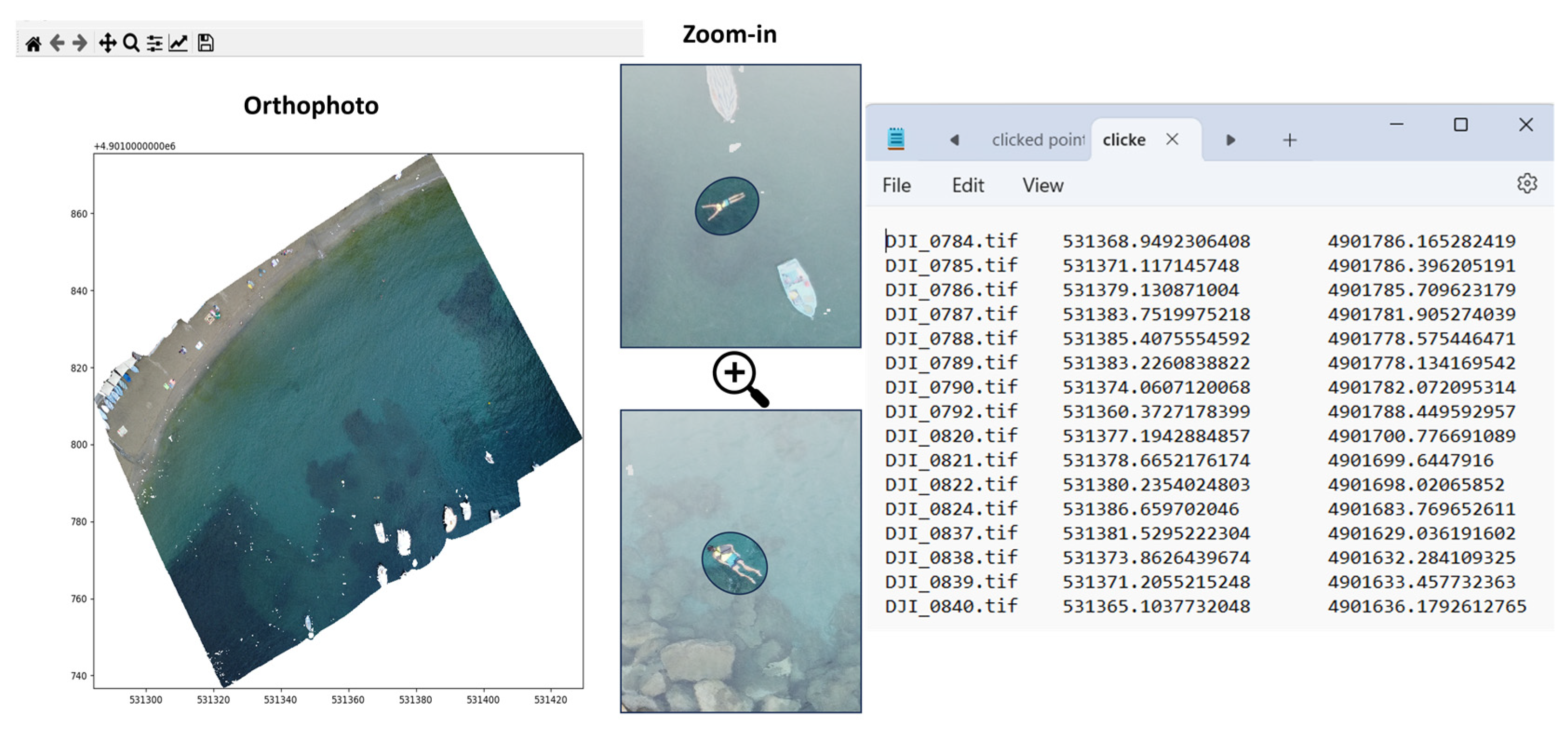
3.1.1. Orthophoto as Bridge
3.1.2. User Friendly Application
3.2. Underwater Photogrammetric Model
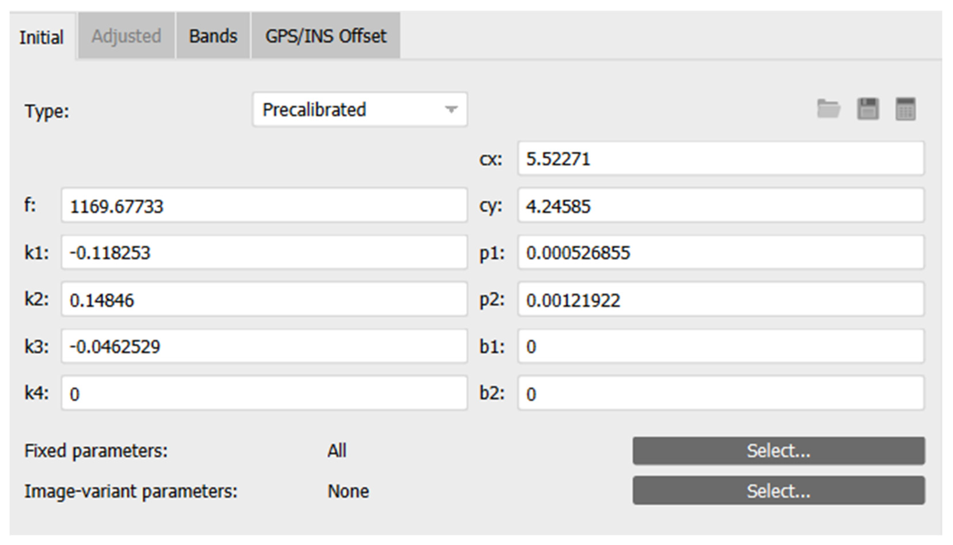
3.2.1. Camera Calibration
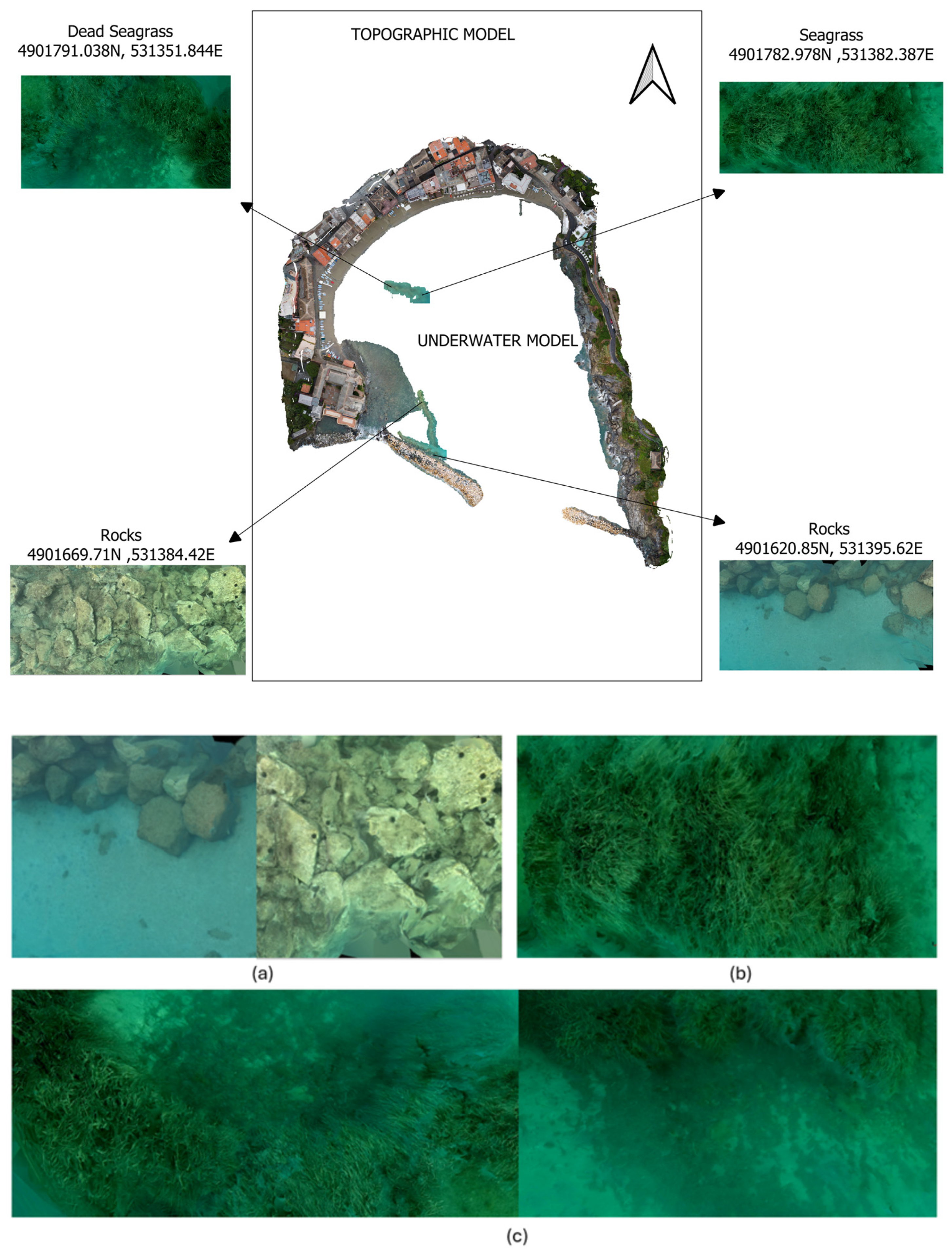
3.2.2. Underwater Georeferenced Model
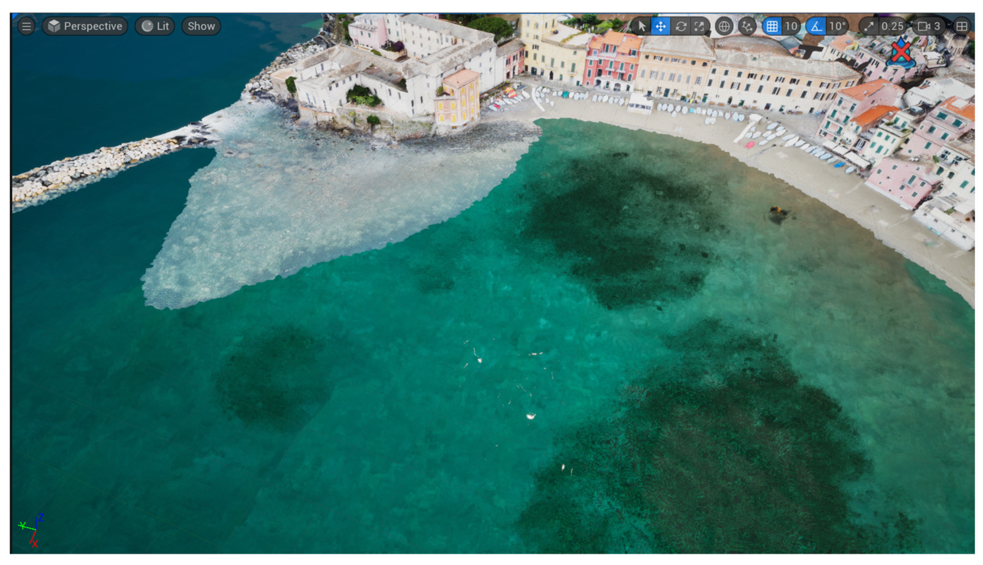
3.3. Merged Model
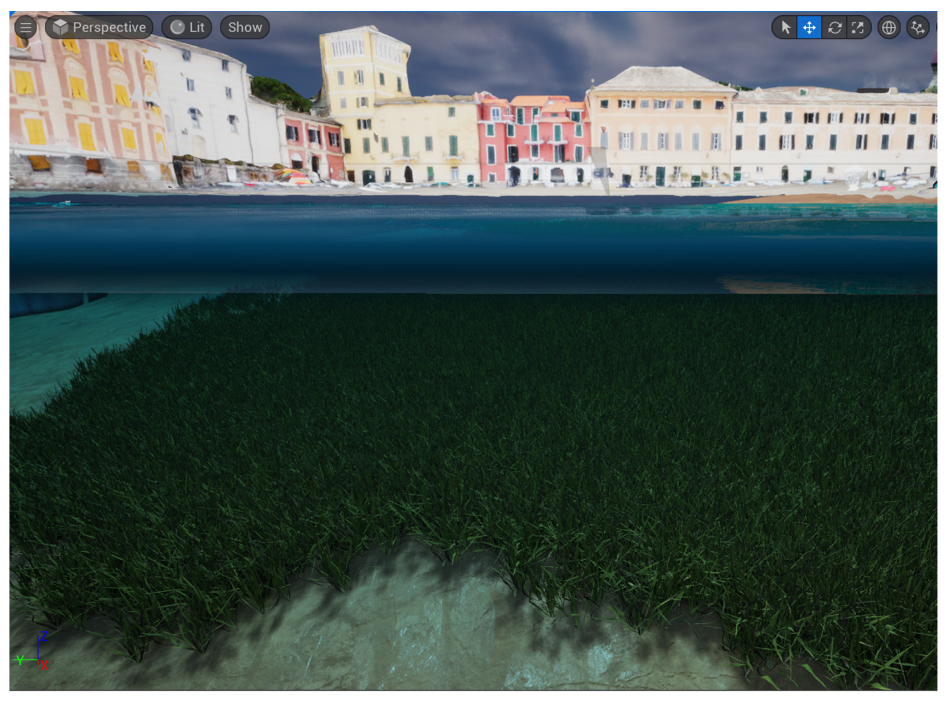
3.4. Virtual Model
4. Discussion
5. Conclusions
Author Contributions
Funding
Data Availability Statement
Acknowledgments
Conflicts of Interest
References
- Bonaldo, D.; Antonioli, F.; Archetti, R.; Bezzi, A.; Correggiari, A.; Davolio, S.; De Falco, G.; Fantini, M.; Fontolan, G.; Furlani, S.; et al. Integrating multidisciplinary instruments for assessing coastal vulnerability to erosion and sea level rise: Lessons and challenges from the Adriatic Sea, Italy. J. Coast. Conserv. 2019, 23, 19–37. [Google Scholar] [CrossRef]
- Teague, J.; Scott, T. Underwater Photogrammetry and 3D Reconstruction of Submerged Objects in Shallow Environments by ROV and Underwater GPS. J. Mar. Sci. Res. Technol. 2017, 1, 005. Available online: https://core.ac.uk/download/pdf/132613751.pdf (accessed on 5 July 2024).
- Fan, J.; Wang, X.; Zhou, C.; Ou, Y.; Jing, F.; Hou, Z. Development, Calibration, and Image Processing of Underwater Structured Light Vision System: A Survey. IEEE Trans. Instrum. Meas. 2023, 72, 5004418. [Google Scholar] [CrossRef]
- Calantropio, A.; Chiabrando, F. Underwater Cultural Heritage Documentation Using Photogrammetry. J. Mar. Sci. Eng. 2024, 12, 413. [Google Scholar] [CrossRef]
- Gallina, V.; Torresan, S.; Critto, A.; Sperotto, A.; Glade, T.; Marcomini, A. A review of multi-risk methodologies for natural hazards: Consequences and challenges for a climate change impact assessment. J. Environ. Manag. 2016, 168, 123–132. [Google Scholar] [CrossRef] [PubMed]
- Pulido Mantas, T.; Roveta, C.; Calcinai, B.; Di Camillo, C.G.; Gambardella, C.; Gregorin, C.; Coppari, M.; Marrocco, T.; Puce, S.; Riccardi, A.; et al. Photogrammetry, from the Land to the Sea and Beyond: A Unifying Approach to Study Terrestrial and Marine Environments. J. Mar. Sci. Eng. 2023, 11, 759. [Google Scholar] [CrossRef]
- McFadden, L. Governing Coastal Spaces: The Case of Disappearing Science in Integrated Coastal Zone Management. Coast. Manag. 2007, 35, 429–443. [Google Scholar] [CrossRef]
- Masselink, G.; Lazarus, E.D. Defining Coastal Resilience. Water 2019, 11, 2587. [Google Scholar] [CrossRef]
- National Academies of Sciences, Engineering, and Medicine; Division of Behavioral and Social Sciences and Education; Division on Earth and Life Studies; Board on Environmental Change and Society; Ocean Studies Board; Board on Earth Sciences and Resources; Committee on Long-Term Coastal Zone Dynamics. Understanding the Long-Term Evolution of the Coupled Natural-Human Coastal System: The Future of the U.S. Gulf Coast; National Academies Press: Washington, DC, USA, 2018; ISBN 978-0-309-47584-6. [Google Scholar]
- Ferrando, I.; Brandolini, P.; Federici, B.; Lucarelli, A.; Sguerso, D.; Morelli, D.; Corradi, N. Coastal Modification in Relation to Sea Storm Effects: Application of 3D Remote Sensing Survey in Sanremo Marina (Liguria, NW Italy). Water 2021, 13, 1040. [Google Scholar] [CrossRef]
- Karaki, A.A.; Bibuli, M.; Caccia, M.; Ferrando, I.; Gagliolo, S.; Odetti, A.; Sguerso, D. Multi-Platforms and Multi-Sensors Integrated Survey for the Submerged and Emerged Areas. J. Mar. Sci. Eng. 2022, 10, 753. [Google Scholar] [CrossRef]
- Alexander, K.A.; Hobday, A.J.; Cvitanovic, C.; Ogier, E.; Nash, K.L.; Cottrell, R.S.; Fleming, A.; Fudge, M.; Fulton, E.A.; Frusher, S.; et al. Progress in integrating natural and social science in marine ecosystem-based management research. Mar. Freshw. Res. 2018, 70, 71–83. [Google Scholar] [CrossRef]
- Holm, P.; Goodsite, M.E.; Cloetingh, S.; Agnoletti, M.; Moldan, B.; Lang, D.J.; Leemans, R.; Moeller, J.O.; Buendía, M.P.; Pohl, W.; et al. Collaboration between the natural, social and human sciences in Global Change Research. Environ. Sci. Policy 2013, 28, 25–35. [Google Scholar] [CrossRef]
- Spooner, E.; Karnauskas, M.; Harvey, C.J.; Kelble, C.; Rosellon-Druker, J.; Kasperski, S.; Lucey, S.M.; Andrews, K.S.; Gittings, S.R.; Moss, J.H.; et al. Using Integrated Ecosystem Assessments to Build Resilient Ecosystems, Communities, and Economies. Coast. Manag. 2021, 49, 26–45. [Google Scholar] [CrossRef]
- Gonçalves, G.; Andriolo, U.; Pinto, L.; Bessa, F. Mapping marine litter using UAS on a beach-dune system: A multidisciplinary approach. Sci. Total Environ. 2020, 706, 135742. [Google Scholar] [CrossRef] [PubMed]
- Cardoso-Andrade, M.; Queiroga, H.; Rangel, M.; Sousa, I.; Belackova, A.; Bentes, L.; Oliveira, F.; Monteiro, P.; Sales Henriques, N.; Afonso, C.M.L.; et al. Setting Performance Indicators for Coastal Marine Protected Areas: An Expert-Based Methodology. Front. Mar. Sci. 2022, 9, 848039. [Google Scholar] [CrossRef]
- Bini, M.; Rossi, V. Climate Change and Anthropogenic Impact on Coastal Environments. Water 2021, 13, 1182. [Google Scholar] [CrossRef]
- van Dongeren, A.; Ciavola, P.; Martinez, G.; Viavattene, C.; Bogaard, T.; Ferreira, O.; Higgins, R.; McCall, R. Introduction to RISC-KIT: Resilience-increasing strategies for coasts. Coast. Eng. 2018, 134, 2–9. [Google Scholar] [CrossRef]
- Clement, S.; Jozaei, J.; Mitchell, M.; Allen, C.R.; Garmestani, A.S. How resilience is framed matters for governance of coastal social-ecological systems. Environ. Policy Gov. 2024, 34, 65–76. [Google Scholar] [CrossRef] [PubMed]
- Talubo, J.P.; Morse, S.; Saroj, D. Whose resilience matters? A socio-ecological systems approach to defining and assessing disaster resilience for small islands. Environ. Chall. 2022, 7, 100511. [Google Scholar] [CrossRef]
- Flood, S.; Schechtman, J. The rise of resilience: Evolution of a new concept in coastal planning in Ireland and the US. Ocean Coast. Manag. 2014, 102, 19–31. [Google Scholar] [CrossRef]
- Chaffin, B.C.; Scown, M. Social-ecological resilience and geomorphic systems. Geomorphology 2018, 305, 221–230. [Google Scholar] [CrossRef]
- Hamal, S.N.G. Investigation of Underwater Photogrammetry Method: Challenges and Photo Capturing Scenarios of the Method. Adv. Underw. Sci. 2023, 3, 19–25. [Google Scholar]
- Abadie, A.; Boissery, P.; Viala, C. Georeferenced underwater photogrammetry to map marine habitats and submerged artificial structures. Photogramm. Rec. 2018, 33, 448–469. [Google Scholar] [CrossRef]
- Marín-Buzón, C.; Pérez-Romero, A.; López-Castro, J.L.; Ben Jerbania, I.; Manzano-Agugliaro, F. Photogrammetry as a New Scientific Tool in Archaeology: Worldwide Research Trends. Sustainability 2021, 13, 5319. [Google Scholar] [CrossRef]
- Rossi, P.; Castagnetti, C.; Capra, A.; Brooks, A.J.; Mancini, F. Detecting change in coral reef 3D structure using underwater photogrammetry: Critical issues and performance metrics. Appl. Geomat. 2020, 12, 3–17. [Google Scholar] [CrossRef]
- Pace, L.A.; Saritas, O.; Deidun, A. Exploring future research and innovation directions for a sustainable blue economy. Mar. Policy 2023, 148, 105433. [Google Scholar] [CrossRef]
- Penca, J.; Barbanti, A.; Cvitanovic, C.; Hamza-Chaffai, A.; Elshazly, A.; Jouffray, J.-B.; Mejjad, N.; Mokos, M. Building competences for researchers working towards ocean sustainability. Mar. Policy 2024, 163, 106132. [Google Scholar] [CrossRef]
- Gill, J.C.; Smith, M. Geosciences and the Sustainable Development Goals; Springer Nature: Berlin, Germany, 2021; ISBN 978-3-030-38815-7. [Google Scholar]
- Ventura, D.; Bonifazi, A.; Gravina, M.F.; Belluscio, A.; Ardizzone, G. Mapping and Classification of Ecologically Sensitive Marine Habitats Using Unmanned Aerial Vehicle (UAV) Imagery and Object-Based Image Analysis (OBIA). Remote Sens. 2018, 10, 1331. [Google Scholar] [CrossRef]
- Wright, A.E.; Conlin, D.L.; Shope, S.M. Assessing the Accuracy of Underwater Photogrammetry for Archaeology: A Comparison of Structure from Motion Photogrammetry and Real Time Kinematic Survey at the East Key Construction Wreck. J. Mar. Sci. Eng. 2020, 8, 849. [Google Scholar] [CrossRef]
- Marre, G.; Holon, F.; Luque, S.; Boissery, P.; Deter, J. Monitoring Marine Habitats With Photogrammetry: A Cost-Effective, Accurate, Precise and High-Resolution Reconstruction Method. Front. Mar. Sci. 2019, 6, 276. [Google Scholar] [CrossRef]
- Prahov, N.; Prodanov, B.; Dimitrov, K.; Dimitrov, L.; Velkovsky, K. Application of Aerial Photogrammetry in the Study of the Underwater Archaeological Heritage of Nessebar. In Proceedings of the 20th International Multidisciplinary Scientific GeoConference SGEM 2020, Albena, Bulgaria, 16–25 August 2020; pp. 175–182. [Google Scholar] [CrossRef]
- Russo, F.; Del Pizzo, S.; Di Ciaccio, F.; Troisi, S. Monitoring the Posidonia Meadows structure through underwater photogrammetry: A case study. In Proceedings of the 2022 IEEE International Workshop on Metrology for the Sea; Learning to Measure Sea Health Parameters (MetroSea), Milazzo, Italy, 3–5 October 2022; pp. 215–219. [Google Scholar] [CrossRef]
- Arnaubec, A.; Ferrera, M.; Escartín, J.; Matabos, M.; Gracias, N.; Opderbecke, J. Underwater 3D Reconstruction from Video or Still Imagery: Matisse and 3DMetrics Processing and Exploitation Software. J. Mar. Sci. Eng. 2023, 11, 985. [Google Scholar] [CrossRef]
- Nocerino, E.; Menna, F.; Gruen, A.; Troyer, M.; Capra, A.; Castagnetti, C.; Rossi, P.; Brooks, A.J.; Schmitt, R.J.; Holbrook, S.J. Coral Reef Monitoring by Scuba Divers Using Underwater Photogrammetry and Geodetic Surveying. Remote Sens. 2020, 12, 3036. [Google Scholar] [CrossRef]
- Hains, D.; Schiller, L.; Ponce, R.; Bergmann, M.; Cawthra, H.C.; Cove, K.; Echeverry, P.; Gaunavou, L.; Kim, S.-P.; Lavagnino, A.C.; et al. Hydrospatial—Update and progress in the definition of this term. Int. Hydrogr. Rev. 2022, 28, 221–225. [Google Scholar] [CrossRef]
- Davila Delgado, J.M.; Oyedele, L. Digital Twins for the built environment: Learning from conceptual and process models in manufacturing. Adv. Eng. Inform. 2021, 49, 101332. [Google Scholar] [CrossRef]
- Madusanka, N.S.; Fan, Y.; Yang, S.; Xiang, X. Digital Twin in the Maritime Domain: A Review and Emerging Trends. J. Mar. Sci. Eng. 2023, 11, 1021. [Google Scholar] [CrossRef]
- Riaz, K.; McAfee, M.; Gharbia, S.S. Management of Climate Resilience: Exploring the Potential of Digital Twin Technology, 3D City Modelling, and Early Warning Systems. Sensors 2023, 23, 2659. [Google Scholar] [CrossRef] [PubMed]
- Stern, P.C. Understanding Individuals’ Environmentally Significant Behavior. Environ. Law. Report. News Anal. 2005, 35, 10785. [Google Scholar]
- Hofman, K.; Walters, G.; Hughes, K. The effectiveness of virtual vs real-life marine tourism experiences in encouraging conservation behaviour. J. Sustain. Tour. 2022, 30, 742–766. [Google Scholar] [CrossRef]
- Kelly, R.; Evans, K.; Alexander, K.; Bettiol, S.; Corney, S.; Cullen-Knox, C.; Cvitanovic, C.; de Salas, K.; Emad, G.R.; Fullbrook, L.; et al. Connecting to the oceans: Supporting ocean literacy and public engagement. Rev. Fish Biol. Fish. 2022, 32, 123–143. [Google Scholar] [CrossRef]
- Wang, Z. Influence of Climate Change On Marine Species and Its Solutions. IOP Conf. Ser. Earth Environ. Sci. 2022, 1011, 012053. [Google Scholar] [CrossRef]
- Ferreira, J.C.; Vasconcelos, L.; Monteiro, R.; Silva, F.Z.; Duarte, C.M.; Ferreira, F. Ocean Literacy to Promote Sustainable Development Goals and Agenda 2030 in Coastal Communities. Educ. Sci. 2021, 11, 62. [Google Scholar] [CrossRef]
- He, J.; Lin, J.; Ma, M.; Liao, X. Mapping topo-bathymetry of transparent tufa lakes using UAV-based photogrammetry and RGB imagery. Geomorphology 2021, 389, 107832. [Google Scholar] [CrossRef]
- Mazza, D.; Parente, L.; Cifaldi, D.; Meo, A.; Senatore, M.R.; Guadagno, F.M.; Revellino, P. Quick bathymetry mapping of a Roman archaeological site using RTK UAS-based photogrammetry. Front. Earth Sci. 2023, 11, 1183982. [Google Scholar] [CrossRef]
- Apicella, L.; De Martino, M.; Ferrando, I.; Quarati, A.; Federici, B. Deriving Coastal Shallow Bathymetry from Sentinel 2-, Aircraft- and UAV-Derived Orthophotos: A Case Study in Ligurian Marinas. J. Mar. Sci. Eng. 2023, 11, 671. [Google Scholar] [CrossRef]
- Jaud, M.; Delsol, S.; Urbina-Barreto, I.; Augereau, E.; Cordier, E.; Guilhaumon, F.; Le Dantec, N.; Floc’h, F.; Delacourt, C. Low-Tech and Low-Cost System for High-Resolution Underwater RTK Photogrammetry in Coastal Shallow Waters. Remote Sens. 2023, 16, 20. [Google Scholar] [CrossRef]
- Kahmen, O.; Rofallski, R.; Luhmann, T. Impact of Stereo Camera Calibration to Object Accuracy in Multimedia Photogrammetry. Remote Sens. 2020, 12, 2057. [Google Scholar] [CrossRef]
- Remmers, T.; Grech, A.; Roelfsema, C.; Gordon, S.; Lechene, M.; Ferrari, R. Close-range underwater photogrammetry for coral reef ecology: A systematic literature review. Coral Reefs 2024, 43, 35–52. [Google Scholar] [CrossRef]
- Calantropio, A.; Chiabrando, F. Georeferencing Strategies in Very Shallow Waters: A Novel GCPs Survey Approach for UCH Photogrammetric Documentation. Remote Sens. 2024, 16, 1313. [Google Scholar] [CrossRef]
- Del Savio, A.A.; Luna Torres, A.; Vergara Olivera, M.A.; Llimpe Rojas, S.R.; Urday Ibarra, G.T.; Neckel, A. Using UAVs and Photogrammetry in Bathymetric Surveys in Shallow Waters. Appl. Sci. 2023, 13, 3420. [Google Scholar] [CrossRef]
- Ventura, D.; Castoro, L.; Mancini, G.; Casoli, E.; Pace, D.S.; Belluscio, A.; Ardizzone, G. High spatial resolution underwater data for mapping seagrass transplantation: A powerful tool for visualization and analysis. Data Brief 2022, 40, 107735. [Google Scholar] [CrossRef] [PubMed]
- Wang, E.; Li, D.; Wang, Z.; Cao, W.; Zhang, J.; Wang, J.; Zhang, H. Pixel-level bathymetry mapping of optically shallow water areas by combining aerial RGB video and photogrammetry. Geomorphology 2024, 449, 109049. [Google Scholar] [CrossRef]
- Marre, G.; Deter, J.; Holon, F.; Boissery, P.; Luque, S. Fine-scale automatic mapping of living Posidonia oceanica seagrass beds with underwater photogrammetry. Mar. Ecol. Prog. Ser. 2020, 643, 63–74. [Google Scholar] [CrossRef]
- Menna, F.; Nocerino, E.; Drap, P.; Remondino, F.; Murtiyoso, A.; Grussenmeyer, P.; Börlin, N. IMPROVING UNDERWATER ACCURACY BY EMPIRICAL WEIGHTING OF IMAGE OBSERVATIONS. Int. Arch. Photogramm. Remote Sens. Spat. Inf. Sci. 2018, XLII–2, 699–705. [Google Scholar] [CrossRef]
- Federici, B.; Corradi, N.; Ferrando, I.; Sguerso, D.; Lucarelli, A.; Guida, S.; Brandolini, P. Remote sensing techniques applied to geomorphological mapping of rocky coast: The case study of Gallinara Island (Western Liguria, Italy). Eur. J. Remote Sens. 2019, 52, 123–136. [Google Scholar] [CrossRef]
- Menna, F.; Nocerino, E.; Nawaf, M.M.; Seinturier, J.; Torresani, A.; Drap, P.; Remondino, F.; Chemisky, B. Towards real-time underwater photogrammetry for subsea metrology applications. In Proceedings of the OCEANS 2019—Marseille, Marseilles, France, 17–20 June 2019; IEEE: Marseille, France, 2019; pp. 1–10. [Google Scholar] [CrossRef]
- Capra, A.; Castagnetti, C.; Mancini, F.; Rossi, P. Underwater Photogrammetry for Change Detection. In Proceedings of the FIG Working Week, Amsterdam, The Netherlands, 10–14 May 2020. [Google Scholar]
- Russo, F.; Del Pizzo, S.; Di Ciaccio, F.; Troisi, S. An Enhanced Photogrammetric Approach for the Underwater Surveying of the Posidonia Meadow Structure in the Spiaggia Nera Area of Maratea. J. Imaging 2023, 9, 113. [Google Scholar] [CrossRef] [PubMed]
- Hochschild, V.; Braun, A.; Sommer, C.; Warth, G.; Omran, A. Visualizing Landscapes by Geospatial Techniques. In Modern Approaches to the Visualization of Landscapes; Edler, D., Jenal, C., Kühne, O., Eds.; Springer Fachmedien: Wiesbaden, Germany, 2020; pp. 47–78. ISBN 978-3-658-30956-5. [Google Scholar] [CrossRef]
- Bayomi, N.; Fernandez, J.E. Eyes in the Sky: Drones Applications in the Built Environment under Climate Change Challenges. Drones 2023, 7, 637. [Google Scholar] [CrossRef]
- Ferrando, I.; Berrino, E.; Federici, B.; Gagliolo, S.; Sguerso, D. Photogrammetric Processing and Fruition of Products in Open-Source Environment Applied to the Case Study of the Archaeological Park of Pompeii. Int. Arch. Photogramm. Remote Sens. Spat. Inf. Sci. 2022, XLVIII-4-W1-2022, 143–149. [Google Scholar] [CrossRef]
- Vacca, G.; Vecchi, E. UAV Photogrammetric Surveys for Tree Height Estimation. Drones 2024, 8, 106. [Google Scholar] [CrossRef]
- Nocerino, E.; Menna, F. Photogrammetry: Linking the World across the Water Surface. J. Mar. Sci. Eng. 2020, 8, 128. [Google Scholar] [CrossRef]
- Pulido Mantas, T.; Roveta, C.; Calcinai, B.; Coppari, M.; Di Camillo, C.G.; Marchesi, V.; Marrocco, T.; Puce, S.; Cerrano, C. Photogrammetry as a promising tool to unveil marine caves’ benthic assemblages. Sci. Rep. 2023, 13, 7587. [Google Scholar] [CrossRef] [PubMed]
- Eltner, A.; Sofia, G. Chapter 1—Structure from motion photogrammetric technique. In Developments in Earth Surface Processes; Tarolli, P., Mudd, S.M., Eds.; Remote Sensing of Geomorphology; Elsevier: Amsterdam, The Netherlands, 2020; Volume 23, pp. 1–24. [Google Scholar] [CrossRef]
- Jeon, I.; Lee, I. 3D reconstruction of unstable underwater environment with sfm using slam. Int. Arch. Photogramm. Remote Sens. Spat. Inf. Sci. 2020, XLIII-B2-2020, 957–962. [Google Scholar] [CrossRef]
- Alkhatib, M.N.; Bobkov, A.V.; Zadoroznaya, N.M. Camera pose estimation based on structure from motion. Procedia Comput. Sci. 2021, 186, 146–153. [Google Scholar] [CrossRef]
- Hu, K.; Wang, T.; Shen, C.; Weng, C.; Zhou, F.; Xia, M.; Weng, L. Overview of Underwater 3D Reconstruction Technology Based on Optical Images. J. Mar. Sci. Eng. 2023, 11, 949. [Google Scholar] [CrossRef]
- Wang, X.; Fan, X.; Shi, P.; Ni, J.; Zhou, Z. An Overview of Key SLAM Technologies for Underwater Scenes. Remote Sens. 2023, 15, 2496. [Google Scholar] [CrossRef]
- Ventura, D.; Mancini, G.; Casoli, E.; Pace, D.S.; Lasinio, G.J.; Belluscio, A.; Ardizzone, G. Seagrass restoration monitoring and shallow-water benthic habitat mapping through a photogrammetry-based protocol. J. Environ. Manag. 2022, 304, 114262. [Google Scholar] [CrossRef]
- Hamal, S.N.G.; Ulvi, A.; Yiğit, A.Y. Three-Dimensional Modeling of an Object Using Underwater Photogrammetry. Adv. Underw. Sci. 2021, 1, 11–15. [Google Scholar]
- Nocerino, E.; Menna, F. In-camera IMU angular data for orthophoto projection in underwater photogrammetry. ISPRS Open J. Photogramm. Remote Sens. 2023, 7, 100027. [Google Scholar] [CrossRef]
- Menna, F.; Nocerino, E.; Ural, S.; Gruen, A. MITIGATING IMAGE RESIDUALS SYSTEMATIC PATTERNS IN UNDERWATER PHOTOGRAMMETRY. Int. Arch. Photogramm. Remote Sens. Spat. Inf. Sci. 2020, XLIII-B2-2020, 977–984. [Google Scholar] [CrossRef]
- Neyer, F.; Nocerino, E.; Gruen, A. Image quality improvements in low-cost underwater photogrammetry. ISPRS—Int. Arch. Photogramm. Remote. Sens. Spat. Inf. Sci. 2019, XLII-2/W10, 135–142. [Google Scholar] [CrossRef]
- Nocerino, E.; Nawaf, M.M.; Saccone, M.; Ellefi, M.B.; Pasquet, J. Multi-Camera System Calibration of a Low-Cost Remotely Operated Vehicle for Underwater Cave Exploration. ISPRS—Int. Arch. Photogramm. Remote. Sens. Spat. Inf. Sci. 2018, XLII-1, 329–337. [Google Scholar] [CrossRef]
- She, M.; Song, Y.; Mohrmann, J.; Köser, K. Adjustment and Calibration of Dome Port Camera Systems for Underwater Vision. In Pattern Recognition; Fink, G.A., Frintrop, S., Jiang, X., Eds.; Springer International Publishing: Cham, Switzerland, 2019; Volume 11824, pp. 79–92. ISBN 978-3-030-33675-2. Lecture Notes in Computer Science. [Google Scholar] [CrossRef]
- James, M.R.; Robson, S. Mitigating systematic error in topographic models derived from UAV and ground-based image networks. Earth Surf. Process. Landf. 2014, 39, 1413–1420. [Google Scholar] [CrossRef]
- Ballarin, M.; Costa, E.; Piemonte, A.; Piras, M.; Teppati Losè, L. UNDERWATER PHOTOGRAMMETRY: POTENTIALITIES AND PROBLEMS RESULTS OF THE BENCHMARK SESSION OF THE 2019 SIFET CONGRESS. Int. Arch. Photogramm. Remote Sens. Spat. Inf. Sci. 2020, XLIII-B2-2020, 925–931. [Google Scholar] [CrossRef]
- Agisoft Metashape. Available online: https://www.agisoft.com/ (accessed on 5 July 2024).
- Regione Liguria GNSS Service. Available online: https://geoportal.regione.liguria.it/servizi/rete-gnss-liguria.html (accessed on 11 December 2024).
- Unreal Engine. Available online: https://www.unrealengine.com/en-US (accessed on 5 July 2024).


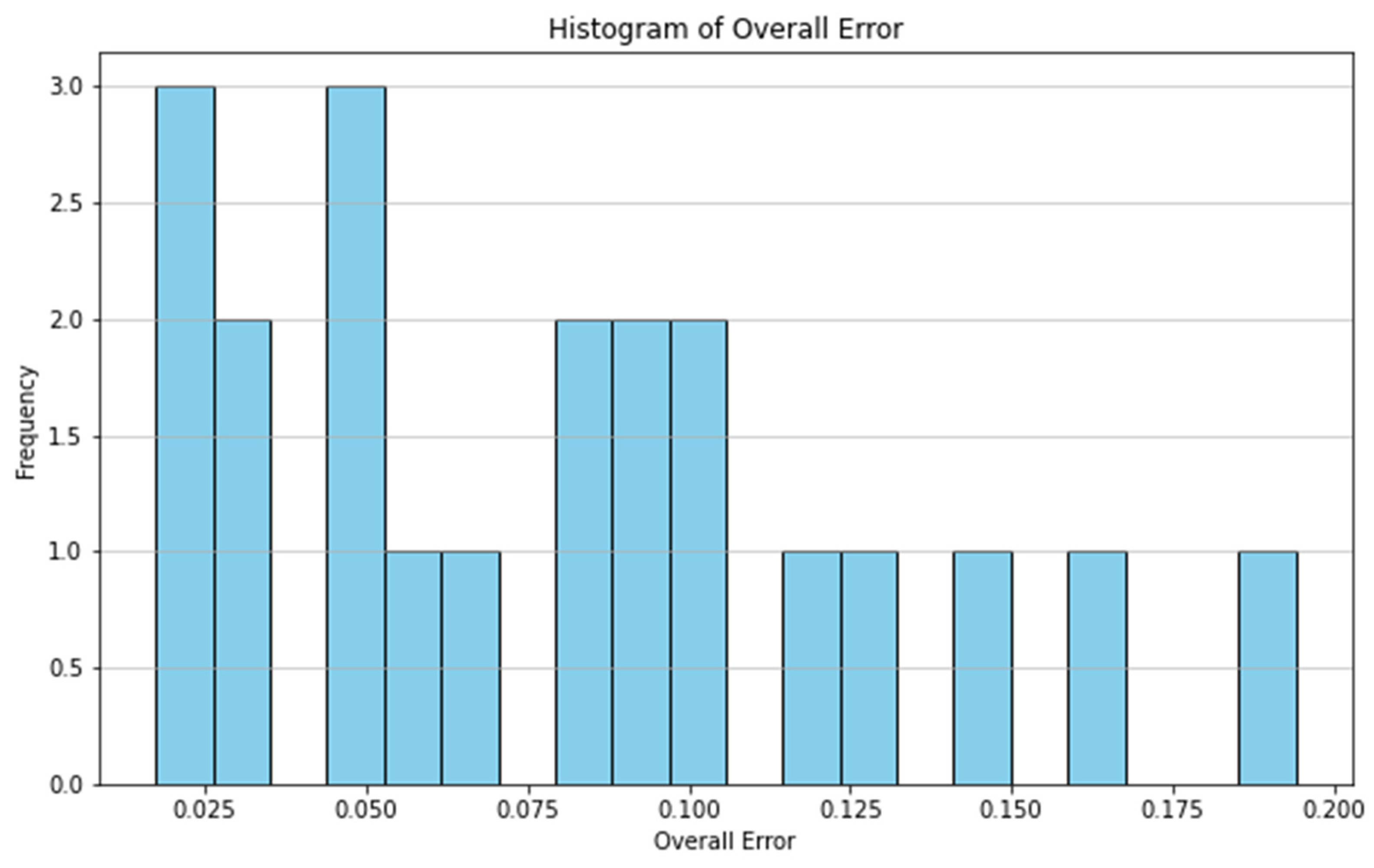
| Error [m] | x | y | Total |
|---|---|---|---|
| Mean | 0.068 | 0.093 | 0.08 |
| Standard deviation | 0.05 | 0.09 | 0.05 |
| Minimum | 0.01 | 0.01 | 0.02 |
| Maximum | 0.16 | 0.34 | 0.19 |
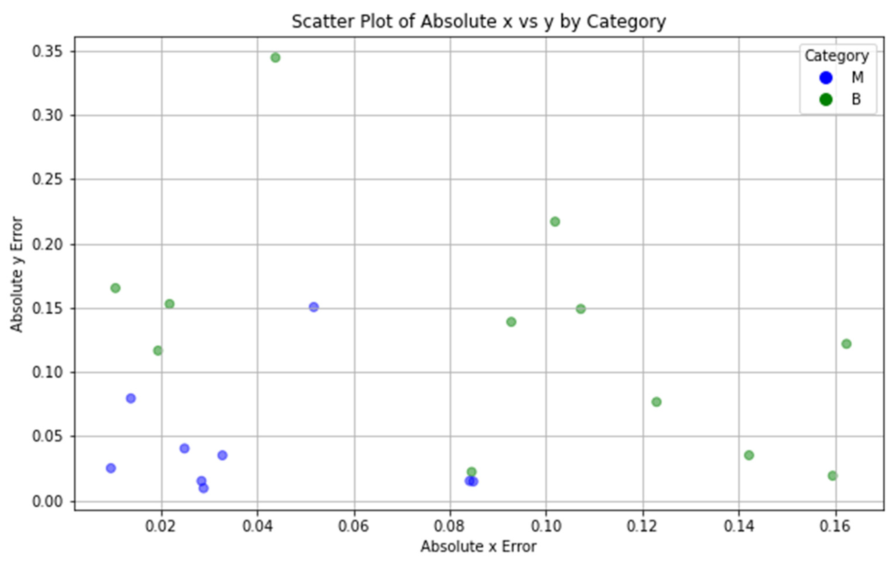
| Error [m] | M | B |
|---|---|---|
| Mean | 0.04 | 0.11 |
| Standard deviation | 0.03 | 0.04 |
| Minimum | 0.02 | 0.05 |
| Maximum | 0.1 | 0.19 |
Disclaimer/Publisher’s Note: The statements, opinions and data contained in all publications are solely those of the individual author(s) and contributor(s) and not of MDPI and/or the editor(s). MDPI and/or the editor(s) disclaim responsibility for any injury to people or property resulting from any ideas, methods, instructions or products referred to in the content. |
© 2024 by the authors. Licensee MDPI, Basel, Switzerland. This article is an open access article distributed under the terms and conditions of the Creative Commons Attribution (CC BY) license (https://creativecommons.org/licenses/by/4.0/).
Share and Cite
Karaki, A.A.; Ferrando, I.; Federici, B.; Sguerso, D. Bridging Disciplines with Photogrammetry: A Coastal Exploration Approach for 3D Mapping and Underwater Positioning. Remote Sens. 2025, 17, 73. https://doi.org/10.3390/rs17010073
Karaki AA, Ferrando I, Federici B, Sguerso D. Bridging Disciplines with Photogrammetry: A Coastal Exploration Approach for 3D Mapping and Underwater Positioning. Remote Sensing. 2025; 17(1):73. https://doi.org/10.3390/rs17010073
Chicago/Turabian StyleKaraki, Ali Alakbar, Ilaria Ferrando, Bianca Federici, and Domenico Sguerso. 2025. "Bridging Disciplines with Photogrammetry: A Coastal Exploration Approach for 3D Mapping and Underwater Positioning" Remote Sensing 17, no. 1: 73. https://doi.org/10.3390/rs17010073
APA StyleKaraki, A. A., Ferrando, I., Federici, B., & Sguerso, D. (2025). Bridging Disciplines with Photogrammetry: A Coastal Exploration Approach for 3D Mapping and Underwater Positioning. Remote Sensing, 17(1), 73. https://doi.org/10.3390/rs17010073