Star Identification Algorithm Based on Dynamic Distance Ratio Matching

Abstract

A star tracker is a widely used celestial sensor in astronomical navigation systems, which calculates the spacecraft’s high-precision attitude by observing stars in space to obtain several star vectors. Existing star identification algorithms typically require the selection of a specific anchor star (e.g., the nearest neighbor star), using the line connecting the target star and the anchor star as the rotational reference axis to achieve rotation invariance in the star identification algorithm. However, this approach makes the entire identification algorithm overly dependent on the anchor star, resulting in insufficient identification accuracy in cases of excessive positional noise or a high number of false stars. In this paper, we adopt the angles between any neighboring stars and the distances ratio between neighboring stars and the observed star as the initial matching criteria. We then calculate the matching with each navigation star using the accumulated angle in the counterclockwise direction based on this criterion. The navigation star with the highest matching is identified. Unlike other identification algorithms that require selecting the nearest neighbor star which can be easily affected by interference as the rotational reference axis, our method effectively achieves rotation invariance in star identification by leveraging angle information. Therefore, it exhibits better tolerance to positional noise, magnitude noise, and false stars, particularly demonstrating higher robustness against focal length variations.

1. Introduction

A star tracker is a celestial sensor used in astronomical navigation systems, characterized by its compact size, high precision, and strong autonomy. It calculates the spacecraft’s attitude by observing stars in space and has been widely applied in the aerospace field. As a key technology of star sensors, star identification algorithms are essential for implementing reliable and rapid star identification, making it an important research topic [1,2,3,4,5].

The triangular algorithm proposed by Liebe et al. [6] utilizes the angular distances between three stars as features for identification. This method is relatively fast but exhibits some redundancy. Mortari et al. [7] extended this approach to include four star points, further reducing redundancy in the identification process. Zhang Guangjun et al. [8] introduced an algorithm based on the navigation star field and K-vectors, accelerating the algorithm using a K-vector lookup table. Wei et al. [9] proposed converting the star image from Cartesian to polar coordinates to achieve scale and rotation invariance in the identification algorithm. Padgett et al. [10] developed a grid-based algorithm for star pattern matching by rasterizing the star image as a feature; however, this algorithm performs poorly under small disturbances such as varying star magnitudes and positional noise. Na et al. [11] replaced the hard template matching in the original raster matching process with a cost function that considers the differences between the measured pattern and database patterns, employing the relative magnitudes of stars as weights to enhance robustness against positional and magnitude noise. Silani et al. [12] introduced the Polestar algorithm, using one star as a reference to calculate angular distances to neighboring stars, forming a specific binary vector and applying a lookup table structure combined with a voting method for identification. Subsequently, Zhang [13] utilized a stepwise identification algorithm, performing initial matching with radial features and subsequent matching with angular features. However, like the grid algorithm, the choice of the starting edge in angular features is susceptible to noise. Wei et al. [14] proposed using the angles between neighboring star vectors as dynamic angular features to mitigate the impact of starting edge selection under noisy conditions. Samirbhai et al. [15] employed a rotation-invariant additive vector as identification features, selecting the best match via voting; however, this method also heavily relies on the selection of the starting star.

The aforementioned identification processes are overly dependent on the starting star, leading to inadequate identification precision in the presence of significant positional noise or numerous false stars. We address this issue by using the angles between arbitrary neighboring stars and the distance ratios between neighboring stars and the observed star as the conditions for initial matching. Subsequently, a cumulative angle calculation method in the counterclockwise direction is employed to assess the matching degree with each navigation star. The star with the highest matching degree is determined to be the correct navigation star, thereby improving the robustness of the star identification algorithm against noise interference.

2. Star Pattern and Catalog

Star identification algorithms are mainly divided into two parts: offline establishment of a star pattern database and online algorithm application. This section primarily focuses on the offline process, which includes the selection of a navigation star pattern and the construction of a star catalog.

2.1. Theory

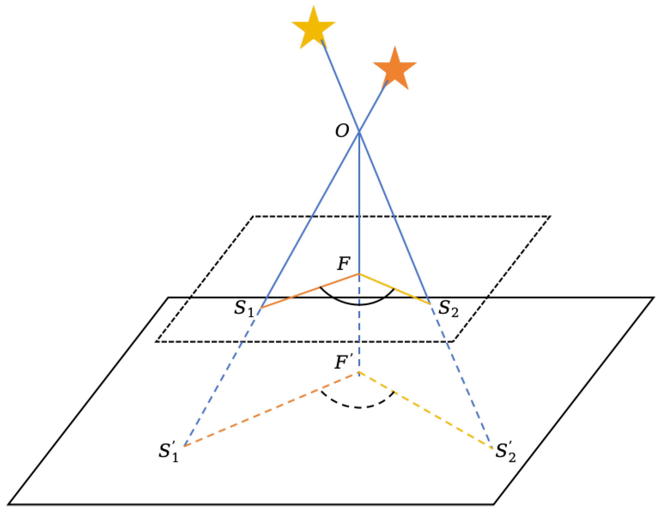
The imaging principle of a star tracker can be approximated as a projection transformation [16]. As shown in Figure 1, star 1 and star 2 are imaged onto the image plane through the lens O, with points F and $F^{\prime }$ representing the center points of the plane. The lengths $OF$ and $O{F}^{\prime }$ correspond to the focal lengths. Due to the variation in focal length, the star points are imaged from $S_1$, $S_2$ to $S_1^{\prime }$, $S_2^{\prime }$ on the image plane.

According to the principle of similar triangles, △$OF{S}_1$ and △$O{F}^{\prime }{S}_1^{\prime }$, △$OF{S}_2$ and △$O{F}^{\prime }{S}_2^{\prime }$ are corresponding similar triangles. Therefore, we can derive the following Equation (1):

$$\left\{\begin{array}{cc}\hfill {\displaystyle \frac{F{S}_1}{F^{\prime }{S}_1^{\prime }}}& ={\displaystyle \frac{F{S}_2}{F^{\prime }{S}_2^{\prime }}}\\ \hfill \angle S_{1}F{S}_2& =\angle S_1^{\prime }{F}^{\prime }{S}_2^{\prime }\end{array}\right.\Rightarrow \left\{\begin{array}{ccc}\hfill d_r& ={\displaystyle \frac{F{S}_1}{F^{\prime }{S}_1^{\prime }}}& ={\displaystyle \frac{F{S}_2}{F^{\prime }{S}_2^{\prime }}}\hfill \\ \hfill \theta & =\angle S_{1}F{S}_2& =\angle S_1^{\prime }{F}^{\prime }{S}_2^{\prime }\hfill \end{array}\right.$$

(1)

In this context, $d_r$ represents the ratio of the distances between the star points on the image plane, and $\theta$ is the angle between the two lines formed by these distances. Both $d_r$ and $\theta$ remain invariant with changes in focal length. Therefore, using {$d_r$, $\theta$} as features in the star identification algorithm can effectively enhance the algorithm’s robustness to variations in focal length and image distortion [17].

2.2. Star Pattern Establishment

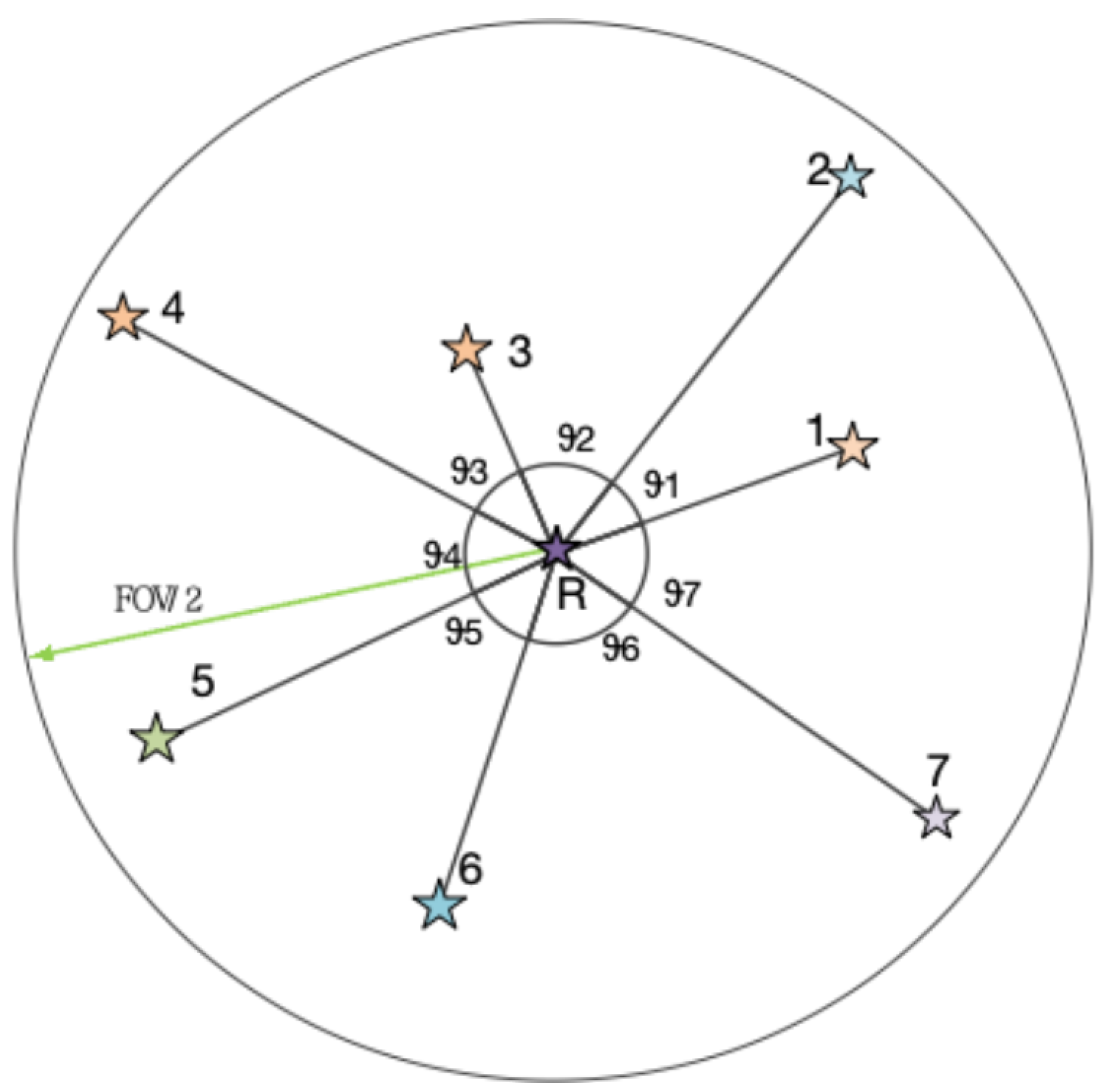
In star identification algorithms, the construction of star pattern features typically involves selecting the navigation star to be identified as the center, with the surrounding stars as neighboring stars for feature construction. As shown in Figure 2, when constructing star pattern features, the navigation star serves as the center of a circle, and half of the field of view $FOV/2$ is used as the radius. This circular area represents the observable region of the celestial sphere that the star sensor can capture when the navigation star is the central axis of view.

In this paper, the distance $r_i$ between the navigation star R and its neighboring stars, along with the angles ${\theta }_i$ between adjacent neighboring stars, are used as the two fundamental features of the navigation star. These features exhibit rotational invariance, making them robust for star identification.

In this region, all stars except the navigation star R are considered neighboring stars. These neighboring stars are labeled in counterclockwise order as {$S_1$, $S_2$, …, $S_n$}, where n represents the total number of neighboring stars. Connecting each neighboring star {$S_1$, $S_2$, …, $S_n$} to the navigation star R, the following Equations (2) and (3) can be used to calculate the distance {$r_1$, $r_2$, …, $r_n$} and angles {${\theta }_1$, ${\theta }_2$, …, ${\theta }_n$}:

$$r_i=\sqrt{{(x_i-x_c)}^2+{(y_i-y_c)}^2}$$

(2)

$${\theta }_i=\left\{\begin{array}{ccc}\hfill arctan\left({\displaystyle \frac{y_{i+1}-y_c}{x_{i+1}-x_c}}\right)-arctan\left({\displaystyle \frac{y_i-y_c}{x_i-x_c}}\right)& \mathrm{for}& i=1,2,\dots ,n-1\hfill \\ \hfill 360-arctan\left({\displaystyle \frac{y_n-y_c}{x_n-x_c}}\right)+arctan\left({\displaystyle \frac{y_1-y_c}{x_1-x_c}}\right)& \mathrm{for}& i=n\hfill \end{array}\right.$$

(3)

where $x_i$ and $y_i$ are the i-th neighbor star coordinates in the image coordinate system, respectively; n is the total neighbor stars in the FOV; and $x_c$ and $y_c$ are the coordinates of the navigation star.

The above features are arranged in a counterclockwise manner. Different starting points $s_i$ correspond to feature vectors $v_r$ and $v_{\theta }$ that are merely cyclically shifted. For example, for navigation star R, the feature vectors $v_r=\{r_1,r_2,\dots ,r_n\}$, $v_{\theta }=\{{\theta }_1,{\theta }_2,\dots ,{\theta }_n\}$ obtained from starting point $s_1$ and the feature vectors $v_r=\{r_6,r_7,\dots ,r_n,\dots ,r_5\}$, $v_{\theta }=\{{\theta }_6,{\theta }_7,\dots ,{\theta }_n,\dots ,{\theta }_5\}$ obtained from another starting point $s_6$ differ only by one cyclic shift. Therefore, using these two features as star pattern features has rotational invariance.

2.3. Star Catalog Generation

We select stars from the SAO J2000 [18] star catalog as navigation stars. Assuming the sensitivity magnitude of the star tracker is set to $6M_v$, then unstable variable stars and difficult-to-distinguish binary stars are removed. Ultimately, 4960 stars are selected as navigation stars. During catalog generation, each of the 4960 stars are taken as the center of the FOV in the star tracker. Based on the size of the FOV, stars that have angular distances within the set FOV are calculated as neighboring stars. This results in $n_{id}$ neighboring stars used to generate the pattern features of the navigation stars. $n_{id}$ is determined by the reference star, which means different stars may have diverse values of $n_{id}$. Generally, the value of $n_{id}$ is greater than 0 and far less than 4960.

Finally, the feature vectors $v_r=\{r_1,r_2,\dots ,r_{n_{id}}\}$, $v_{\theta }=\{{\theta }_1,{\theta }_2,\dots ,{\theta }_{n_{id}}\}$ of each navigation star are obtained and stored in a format shown in

Table 1. Navigation star distance feature.

Star ID	${\mathit{r}}_1$	${\mathit{r}}_2$	…	${\mathit{r}}_{{\mathit{n}}_{\mathbf{id}}}$
1	76.6	425.62	…	129.94
2	127.34	407.67	…	435.60
…	…	…	…	…
4960	128.19	341.2	…	364.03

and

Table 2. Navigation star angle feature.

Star ID	${\mathit{\theta }}_1$	${\mathit{\theta }}_2$	…	${\mathit{\theta }}_{{\mathit{n}}_{\mathbf{id}}}$
1	14.83	6.99	…	70.82
2	15.88	18.74	…	35.66
…	…	…	…	…
4960	51.94	10.84	…	24.26

. The first column contains a unique id for each navigation star, while the subsequent $n_{id}$ columns represent the distance features and angular features corresponding to the $n_{id}$ neighboring stars associated with the current navigation star.

When calculating the distance ratios, the dynamic angles selected are not fixed every time. To enhance the robustness of the algorithm, real-time ratio calculations are employed. Starting from the initial matched angle, each neighboring star’s distance is then computed as a ratio value to the previously matched neighboring star’s distance. This method eliminates variations in star imaging caused by changes in the star tracker’s focal length, and helps prevent issues with false or missing stars that affect identification. Since the distance ratio calculation is dynamic, ratios are computed during the algorithm’s execution rather than being pre-calculated. The specific matching process will be detailed in the following sections.

2.4. Lookup Table Generation

The identification algorithm is divided into two parts: initial matching and similarity calculation. In the initial matching process, we use the distance ratio between the reference star and neighboring stars, as well as the angles between adjacent neighboring stars, as features for subsequent matching. A lookup table (LUT) is generated by precomputing and storing the features of star patterns, including distance ratios and angles, enabling efficient retrieval during the matching process.

According to the feature $\{r_k,{\theta }_k\}$, we construct a two-dimensional lookup table to store stars that share this feature together, thereby reducing redundant matches and further improving the efficiency of initial matching. In this lookup table, the distance ratio $r_k$ and angles ${\theta }_k$ between neighboring stars are discretized as indices $\{i_k,j_k\}$, while the stored values consist of the stars ID $i{d}_{star}$ that possess this feature and the corresponding positions $k_{start}$.

$$i=\lceil {\displaystyle \frac{r_k}{Interva{l}_r}}\rceil$$

(4)

$$j=\lceil {\displaystyle \frac{{\theta }_k}{Interva{l}_{\theta }}}\rceil$$

(5)

$$LUT(i,j)=\{i{d}_{star},k_{start}\}$$

(6)

where $\lceil x\rceil$ denotes the smallest integer greater than a given value, and the intervals for distance and angle partitioning are represented by $interval{s}_r$ and $interval{s}_{\theta }$, respectively. Each time an initial match is performed, the search is reduced to a sufficiently small area. Subsequent matching is then carried out within this reduced search space.

3. Star Identification Algorithm

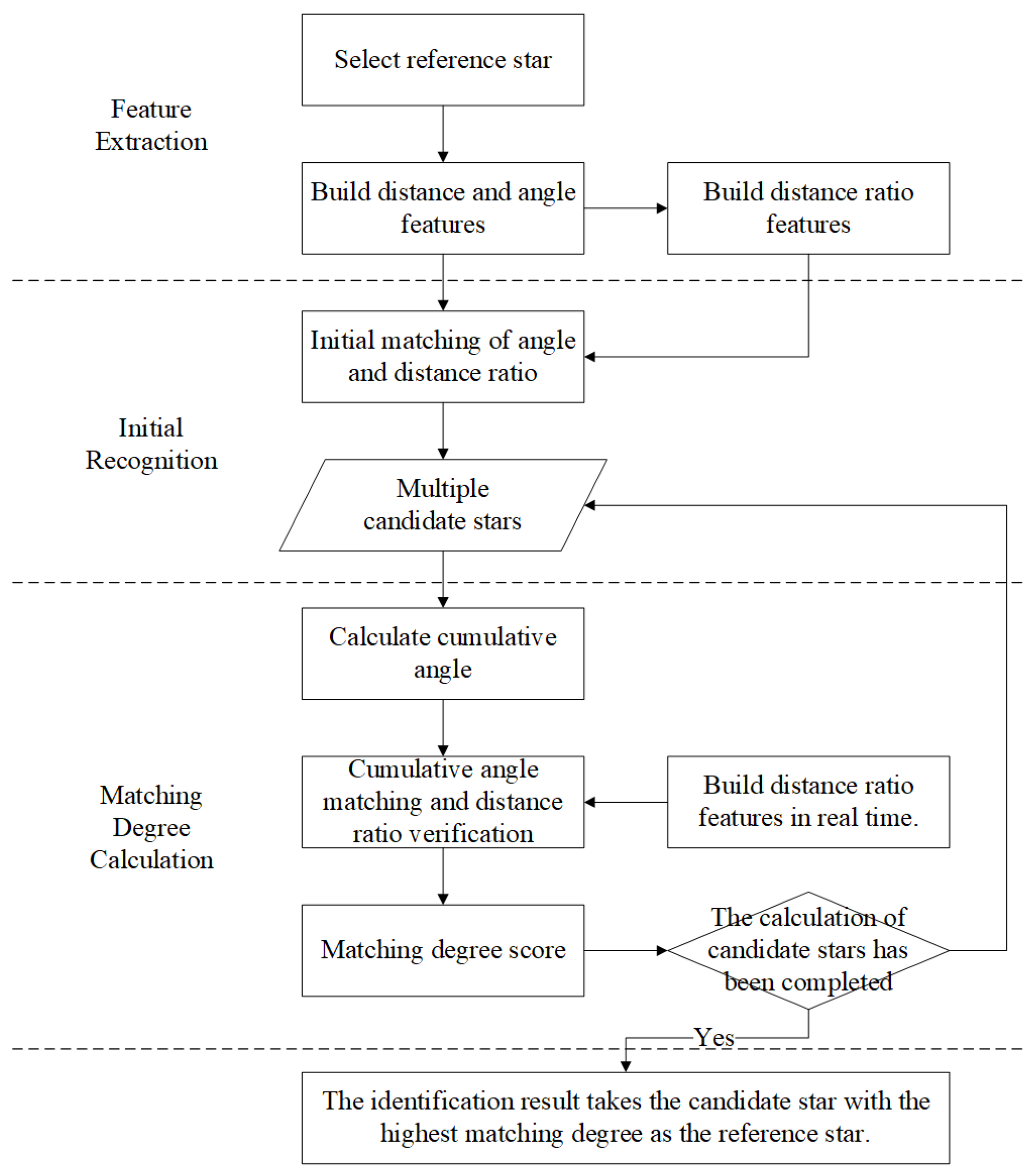
The star identification algorithm is primarily divided into two parts: initial matching and similarity calculation. First, the initial matching process narrows down the range for navigation star identification. Subsequently, among the selected candidate stars, the degree of matching between the reference star and each candidate star is calculated, ultimately selecting the star with the highest matching degree as the result for the reference star.

3.1. Identification Algorithm Flow

In the star identification, the star closest to the center of the FOV is selected as the reference star, and other stars within the FOV are considered neighboring stars. Using these neighboring stars, a star pattern feature is constructed for the reference star, including the distances r between the reference star and its neighboring stars, as well as the angles $\theta$ between each pair of neighboring stars. The distance r between the reference star and neighboring stars varies with changes in focal length. To reduce the dependency of the identification algorithm on an accurate focal length, the distance ratio corresponding to the angle sides is used as an identification feature.

Through the feature extraction, multiple sets of identification features can be obtained. Each feature set serves as starting points for identification. This method overcomes the previous methods’ excessive reliance on the positioning star/reference star, achieving rotational invariance and enhancing robustness against variations in focal length. By expanding from a single match to multiple matches, the overall performance of the algorithm is improved.

After the initial identification of this feature, multiple candidate star combinations that meet the initial matching criteria can be obtained. Next, the matching degree between each candidate star and the reference star to be identified is calculated. Since different starting points may correspond to the same candidate star, multiple matching degree scores may arise. In this case, the highest matching degree score is selected as the final score for that candidate star. Ultimately, the candidate star with the highest matching degree score will be identified as the identification result for the reference star to be identified. The pseudocode is given in Appendix A.

3.2. Initial Identification

During the initial identification process, the star closest to the center of the FOV is selected as the reference star R. As shown in the Figure 2, the reference star R serves as the center of the coordinate system, with other stars (neighboring stars) within the surrounding FOV designated as neighboring stars. Next, the planar distances $\{r_1,r_2,\dots ,r_N\}$ between the reference star and its neighboring stars, as well as the angles $\{{\theta }_1,{\theta }_2,\dots ,{\theta }_N\}$ between each pair of neighboring stars, are calculated sequentially. Based on the planar distances between the reference star and the neighboring stars, the corresponding distance ratios $\{d_{r1},d_{r2},\dots ,d_{r3}\}$ are further obtained.

Using the ratio of distances instead of absolute distances enhances the robustness against focal length variations. Changes in focal length do not affect the distance ratios between the stars.

$$d_{ri}=\left\{\begin{array}{ccc}\hfill {\displaystyle \frac{r_{i+1}}{r_i}}& \mathrm{for}& i=1,2,\dots ,N-1\hfill \\ \\ \hfill {\displaystyle \frac{r_1}{r_N}}& \mathrm{for}& i=N\hfill \end{array}\right.$$

(7)

The distance ratios and angles corresponding to the reference star to be identified are used as initial identification features $\{R_k,{\theta }_k\}$, and a 2D lookup table is utilized to accelerate the search. It is quantified as $\{i,j\}$ according to Equation (6), allowing for rapid identification of candidate navigation stars that meet the criteria through indexing. Simultaneously, to enhance the robustness of the identification algorithm against noise and prevent noise-induced stars from falling into other ranges, the effective candidate star $sta{r}_{condidate}$ search area is expanded to a nine-grid pattern centered around the star $\{i,j\}$ during the search process.

$${\{sta{r}_{id},inde{x}_k\}}_{cod}=\bigcup _{\begin{array}{c}i-1⩽m⩽i+1\\ j-1⩽n⩽j+1\end{array}}LUT(m,n)$$

(8)

After the initial identification process, promising candidate stars that meet the matching requirements have been selected from the navigation star list. Additionally, the corresponding order of the current matching angles with respect to the candidate stars has been established, laying the foundation for the subsequent similarity calculation.

3.3. Matching Calculation

The angles and distance features of the neighboring stars of the reference star R are defined as $ref=\{({\theta }_1,r_1),({\theta }_2,r_2),\dots ,({\theta }_m,r_m)\}$, while the angles and distance features of the neighboring stars of the candidate star $sta{r}_{id}$ are defined as $pa{t}_{id}=\{({\psi }_1,d_1),({\psi }_2,d_2),\dots ,({\psi }_n,d_n)\}$. Here, m and n represent the number of neighboring stars generated for the reference star and the candidate star, respectively.

Through the initial identification process, it can be seen that the k-th adjacent star feature of the reference star is matched with the k-th adjacent star feature of the candidate star. Based on this cumulative angle, the number of feature matches $nu{m}_{match}$ between the reference star R to be identified and the selected candidate star $sta{r}_{id}$ is calculated.

First, the features $ref$ and $pa{t}_{id}$ are cyclically shifted k times and l times, respectively, to obtain $shift\_ref=\{({\alpha }_1,{\beta }_1),({\alpha }_2,{\beta }_2),\dots ,({\alpha }_m,{\beta }_m)\}$, $shift\_pa{t}_{id}=\{(a_1,b_1),(a_2,b_2),\dots ,(a_n,b_n)\}$, and it is easy to know that the starting neighbor features in $shift\_ref$ and $shift\_pa{t}_{id}$ have been matched by $\{{\theta }_k,r_k\}$ and $\{{\psi }_l,d_l\}$, respectively. This satisfies Equation (9):

$$\left\{\begin{array}{c}\hfill ({\alpha }_1,{\beta }_1)\equiv ({\theta }_k,r_k)\\ \hfill (a_1,b_1)\equiv ({\psi }_l,d_l)\end{array}\right.$$

(9)

Based on the cyclic shift features $shift\_ref$ and $shift\_pa{t}_{id}$, and using the angle of them, the cumulative angle features $angl{e}_{ref}=\{{\omega }_1,{\omega }_2,\dots ,{\omega }_m\}$ and $angle\_pa{t}_{id}=\{{\mu }_1,{\mu }_2,\dots ,{\mu }_n\}$ are constructed, and each element is defined as follows:

$$\left\{\begin{array}{cc}\hfill {\omega }_i=\sum _{t=1}^i{\alpha }_t& i\in \{1,2,\dots ,m\}\\ \hfill {\mu }_j=\sum _{t=1}^j{a}_t& j\in \{1,2,\dots ,n\}\end{array}\right.$$

(10)

The $angl{e}_{ref}$ and $angle\_pa{t}_{id}$ could be used for the purpose of match calculations. The closest cumulative angles ${\omega }_i$ and ${\mu }_j$ are taken as the matching candidates pair by traversing through the $angl{e}_{ref}$ and $angle\_pa{t}_{id}$, which satisfies

$$|{\omega }_i-{\mu }_j|\le {\epsilon }_{angle}$$

(11)

where i and j are the i-th element in $angl{e}_{ref}$ and the j-th element in $angle\_pa{t}_{id}$, respectively, and ${\epsilon }_{angle}$ is the threshold for cumulative angle matching. When ${\omega }_i$ and ${\mu }_j$ satisfy Equation (11), only angle information is used. To reduce redundancy in matching, it is also necessary to calculate the current distance ratio as an additional feature for verification.

The calculation of distance ratios is closely related to the selection of comparison objects. To enhance the robustness of the identification algorithm, it is essential not to fix any specific neighboring star as the comparison object. Instead, a dynamic selection method should be used to reduce mutual interference between neighboring stars. In dynamically calculating the distance ratio, the distance between the current neighboring star and the previously successfully matched neighboring star is selected each time to compute the ratio. This method effectively reduces interference from factors such as false stars and missing stars.

Based on the matching results of ${\omega }_i$ and ${\mu }_j$, the corresponding distances ${\beta }_i$ and $b_j$ of the current matching candidate can be obtained. To calculate the distance ratio for the current valid angle, the previously saved distances ${\beta }_{last\_i}$ and $b_{last\_j}$ from the prior match are required. When the distance ratio constraint is satisfied, ${\omega }_i$ and ${\mu }_j$ can be considered successfully matched, i.e.,

$$|{\displaystyle \frac{{\beta }_{last\_i}}{{\beta }_i}}-{\displaystyle \frac{b_{last\_j}}{b_j}}|\le {\epsilon }_R$$

(12)

In the process of calculating the feature match count, i and j start from 1, with the distances ${\beta }_{last\_i}={\beta }_m$ and $b_{last\_i}=b_n$ saved from the previous match. If the features corresponding to i and j match under the cumulative angle and distance ratio constraints, the feature match count $nu{m}_{match}$ between the reference star and the candidate star increases 1, and the current distances ${\beta }_i$ and $b_j$ replace the previously saved distances ${\beta }_{last\_i}$ and $b_{last\_j}$. Then, compare the next position. Otherwise, make the next judgment based on the value of ${\omega }_i$ and ${\mu }_j$ to proceed: if ${\omega }_i<{\mu }_j$, then $i=i+1$; if ${\omega }_i>{\mu }_j$, then $j=j+1$. This process of angle matching accumulation and distance ratio validation continues.

Ultimately, when $i\ge m$ or $j\ge n$ is satisfied, the feature match count calculation ends. The resulting feature match count $nu{m}_{match}$ at this point represents the number of successfully matched neighboring star feature pairs between the reference star R to be identified and the candidate star $sta{r}_{id}$.

Due to differences in the number of neighboring stars around each navigation star, using only the feature match count to measure the matching degree is not reasonable. Therefore, the ratio of the feature match count to the number of neighboring stars around the navigation star should be used as the measure of the matching degree. That is,

$$S={\displaystyle \frac{nu{m}_{match}}{nu{m}_{neighbor}}}$$

(13)

Clearly, the matching score S is in the range of [0,1], where a higher value indicates a greater degree of similarity between the reference star and the current candidate star.

3.4. Algorithm Robustness Analysis

In this section, we illustrate the robustness of the algorithm through a typical identification process. In Figure 3, the filled circle represents the real observed star image, $I_c$ is the center of FOV of star tracker. The star closest to $I_c$ is selected as the reference star R to be identified. In fact, the star pattern feature R is represented as a dashed circular area. As seen in the Figure 3, the current observed star image contains neighboring stars 1, 2, 3, 6, 7, and the false star F. Comparing the ideal neighboring stars 1, 2, 3, 4, 5, 6, and 7 used to construct the star pattern feature R, we find that stars 4 and 5 are missing from the observed star image, while the false star F, which does not exist in the ideal star pattern, is present. The current scene involves the issues of lost stars and multiple stars in stellar identification, which can be used to validate the robustness of the algorithm presented in this paper in handling situations involving missing stars and false stars.

The ideal star patterns of R are $({\theta }_1,{\theta }_2,{\theta }_3,{\theta }_4,{\theta }_5,{\theta }_6,{\theta }_7)$ and $(r_1,r_2,r_3,r_4,r_5,r_6,r_7)$. The actual extracted star patterns are $({\theta }_1,{\theta }_2,{\theta }_3+{\theta }_4+{\theta }_5,{\theta }_{6F},{\theta }_{F7},{\theta }_7)$ and $(r_1,r_2,r_3,r_6,r_F,r_7)$. We randomly select the angle ${\theta }_1$ formed by stars 1 and 2 to create $({\theta }_1,{\displaystyle \frac{r_1}{r_2}})$ as the initial matching feature. This angle ${\theta }_1$ will serve as the starting angle for accumulating angles in the matching degree calculation. The cumulative angle feature of the ideal star model is obtained as $({\theta }_{12},{\theta }_{13},{\theta }_{14},{\theta }_{15},{\theta }_{16},{\theta }_{17},360)$, and the real pattern is $({\theta }_{12},{\theta }_{13},{\theta }_{16},{\theta }_{1F},{\theta }_{17},360)$.

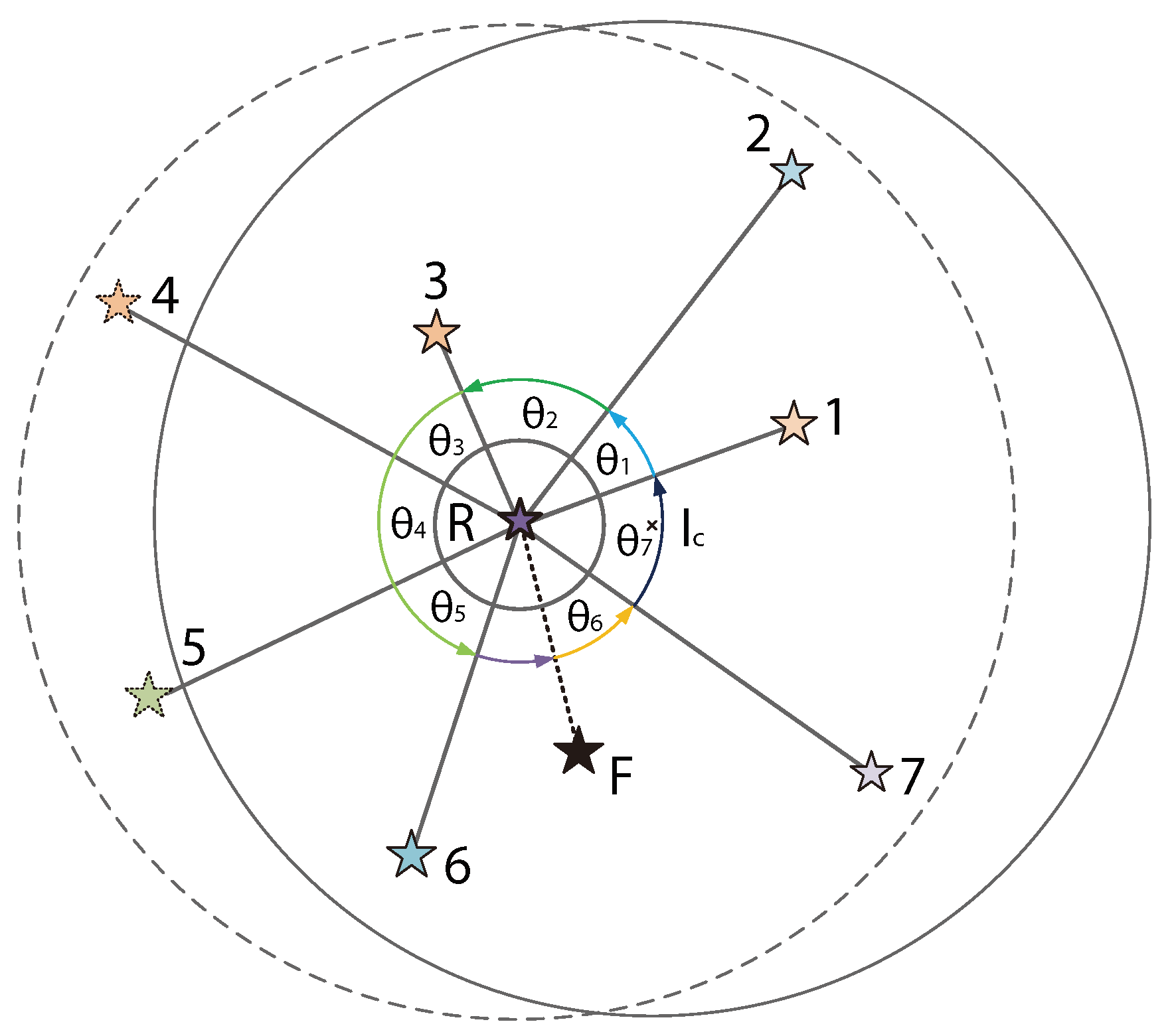
As shown in Figure 4, the current number of neighbor star feature matches is 5. Due to the absence of stars 4 and 5, the accumulated angles ${\theta }_{14}$ and ${\theta }_{15}$ have not completed matching. Additionally, the presence of the false star F has affected the matching of the accumulated angle ${\theta }_{1F}$, which also remains unmatched. However, these two situations do not affect the subsequent matching of neighboring star features. Both stars 6 and 7 complete their matching. Therefore, the proposed algorithm demonstrates strong tolerance to interference from missing stars and false stars.

In addition, to prevent excessive redundancy during the matching process, it is necessary to further verify the dynamic distance ratio after each pair of accumulated angles completes matching. According to previous sections, the distance ratio is independent of focal length, allowing the use of the distance ratio to replace actual distances, thus enhancing the robustness of the identification algorithm against variations in the focal length of the star sensor. When selecting neighboring stars to form the ratio, a dynamic selection method should also be considered.

Figure 5 shows the matching situation using the distance ratios of neighboring angles, with a feature match count of 3. Figure 6 illustrates the method using dynamic distance ratios, where each time the ratio between the current neighboring star’s distance and the distance of the previously matched neighboring star is calculated, resulting in a feature match count of 5. It can be seen that the use of dynamic distance ratios effectively reduces interference from false stars and missing stars. Furthermore, transforming the ratio into a dynamic process enhances the robustness of the algorithm.

4. Supplementation with Adjacent Stars and Distortion Correction

Due to the limitations of optical systems and the degradation of performance during on-orbit operations, actual observed star maps may exhibit various distortions. Typically, the degree of distortion increases with the distance from the center of the image. As a result, in distorted conditions, only a few stars near the center of the field of view can be successfully identified. Additionally, the sparse distribution of some stars or the presence of certain stars in edge regions of the image, where there are fewer neighboring stars providing information, can also lead to incomplete identification.

We propose a method for supplementing neighboring stars by further utilizing the information from various neighboring stars during the matching process to increase the number of identified stars. By employing this method, the actual stars affected can be obtained, while also providing data support for subsequent distortion correction of the star image.

By analyzing the previous stellar identification process, it was found that some neighboring stars’ positional information was not fully utilized. In star identification, the reference star relies on the features provided by its neighboring stars. If the reference star is correctly identified, these neighboring stars should also be uniquely determined. Therefore, when constructing the navigation star catalog, in addition to recording the distance and angle features of each navigation star, it is also necessary to record the corresponding neighboring star numbers in counterclockwise order for each set of features.

The matching process is conducted in a fixed order. When a star is successfully identified, some neighboring stars’ numbers have also been determined throughout the matching process. For the identified navigation star, by combining the order of feature matches during the process and the neighboring star numbers stored in the navigation star database, the true star numbers of each neighboring star can be inferred, thereby restoring these neighboring stars’ numbers sequentially.

Using this method, it is possible to extend the identification from a single recognized star to multiple neighboring stars, significantly increasing the number of identified stars.

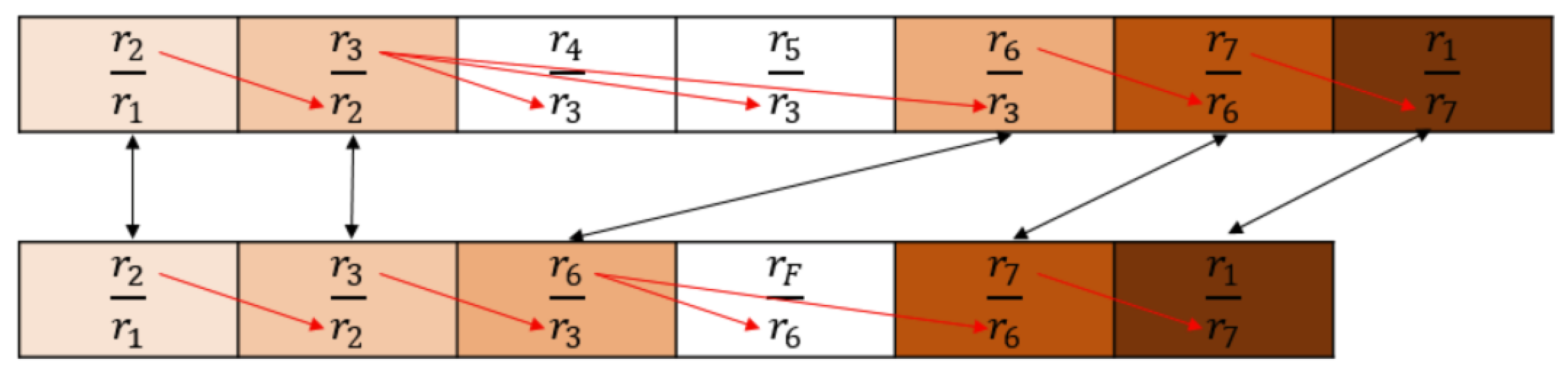
In Figure 7, the left side represents the ideal star pattern, while the right side shows the actual star pattern. As discussed in the previous sections, when the navigation star is correctly identified, the number of neighboring star features that are currently matched is 6, meaning that neighboring stars 1, 2, 4, 5, 6, and 7 have all completed matching.

When constructing the star catalog, the star numbers of each neighboring star are recorded in counterclockwise order, and the matching order is documented during the matching process to derive the theoretical star numbers for neighboring stars 1, 2, 4, 5, 6, and 7. With our method, the number of identified stars can be further expanded.

In our method, it is possible to supplement multiple neighboring star numbers while only identifying one star. Additionally, when multiple stars are recognized, each recognized star can supplement its own neighboring stars, and a neighboring star is considered a valid supplementary star only when the results are consistent across different recognized stars. This approach allows for mutual verification between neighboring stars, further enhancing the reliability of the supplementary neighboring star identification.

Combined with the identification algorithm presented in this paper, the method of neighboring star supplementation can fully utilize the information between various stars, especially in cases where there is significant distortion in star images or a limited number of recognized stars, resulting in a notable improvement in performance.

5. Experiment and Analysis

The simulated star images are used to test the performance of various identification algorithms, selecting some representative star identification algorithms as comparisons for our algorithm. The improved triangle algorithm [8], radial axial algorithm [13], grid algorithm [10], pyramid algorithm [7], and dynamic angle matching [19] are compared with the algorithm presented in this section.

Additionally, to make the simulated star images more closely resemble actual star images, factors such as positional noise, false stars, and magnitude noise are introduced during the simulation process. The identification rates of the algorithms under different conditions are further analyzed to assess their robustness. Finally, real star images transmitted by a specific model of satellite star sensor are used for testing to validate the usability of the algorithm.

All experiments and algorithms were simulated in PyCharm CE (V2021.3) with Python 3.11 on a PC with a 2.30 GHz Intel Xeon Gold 6139 CPU with 32 GB RAM and an NVIDIA Quadro P4000 GPU with 8 GB RAM.

5.1. Generate Simulated Star Images

Stars are selected from the SAO J2000 star catalog, and simulated star images generated using MATLAB 2024 are used to test the algorithm proposed in this paper. The star sensor’s FOV for generating the simulated star images is set to ${12}^{\circ }$ × ${12}^{\circ }$, with an image resolution of 1024 × 1024, pixel size is set to 12 μm, a focal length of $58.4563$ mm, and a sensitive magnitude limit of $6.0$ Mv. During the generation, right ascension and declination are uniformly traversed at $2^{\circ }$ intervals, ultimately resulting in 16,200 simulated star images [15] that evenly cover the entire celestial sphere.

5.2. Position Noise

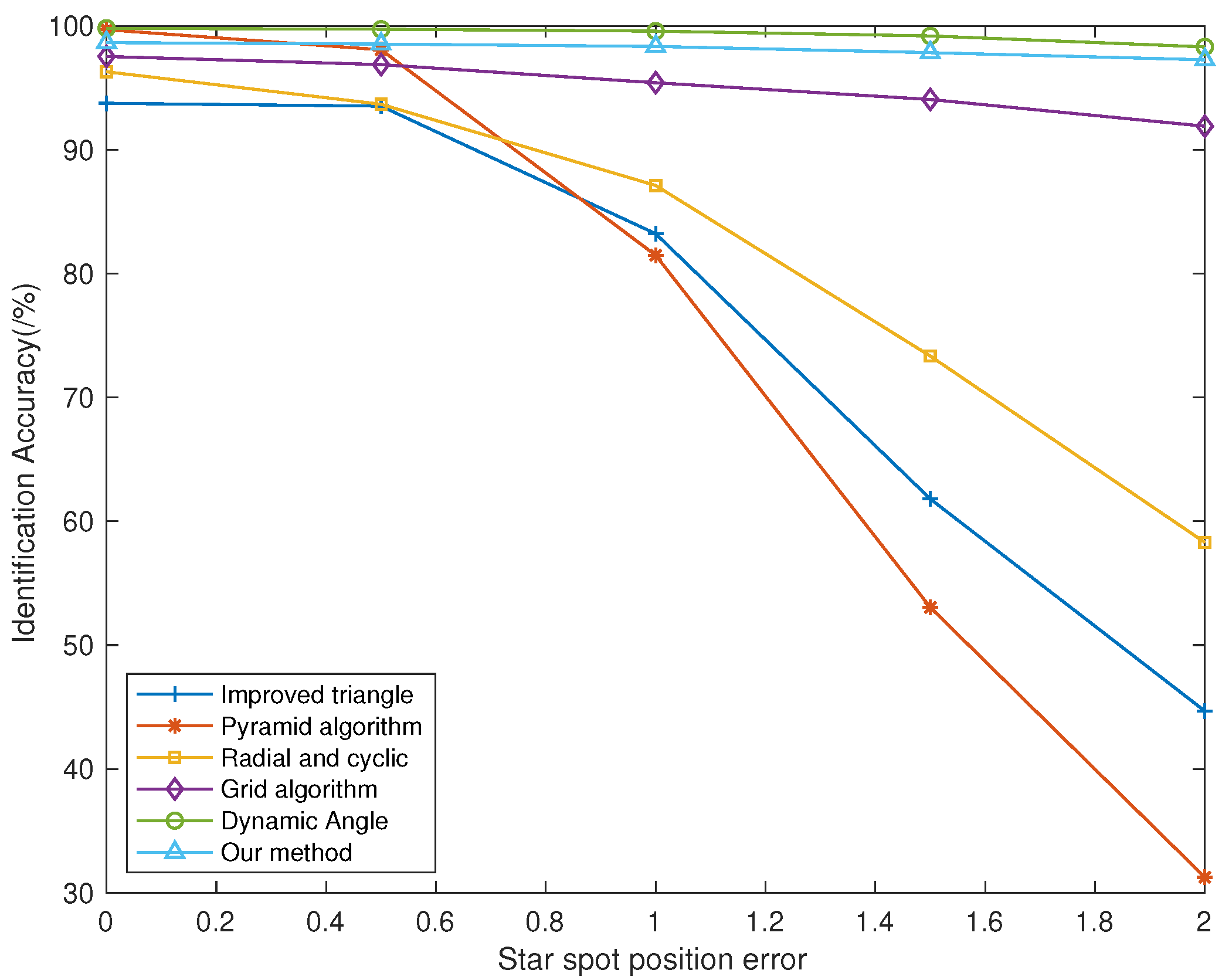
To verify the robustness of various star identification algorithms against positional noise, we added noise with a mean of 0 pixel and a variance ranging from 0 to 2 pixels to the star point coordinates in the simulated star images to observe changes in identification accuracy. As shown in Figure 8, under the influence of positional noise, the identification rates of the improved triangle algorithm, pyramid algorithm, and radial axial algorithm rapidly decline with increasing noise, while the grid algorithm performs slightly better, maintaining a identification rate above 90%. The algorithm based on dynamic angle matching exhibited the highest identification rate. At the same time, the dynamic distance ratio algorithm also showed no significant decrease in recognition rate, maintaining an average recognition rate of 97.26%, even when the star point deviation reached 2 pixels, demonstrating stronger robustness to position noise.

5.3. Pseudo Stars

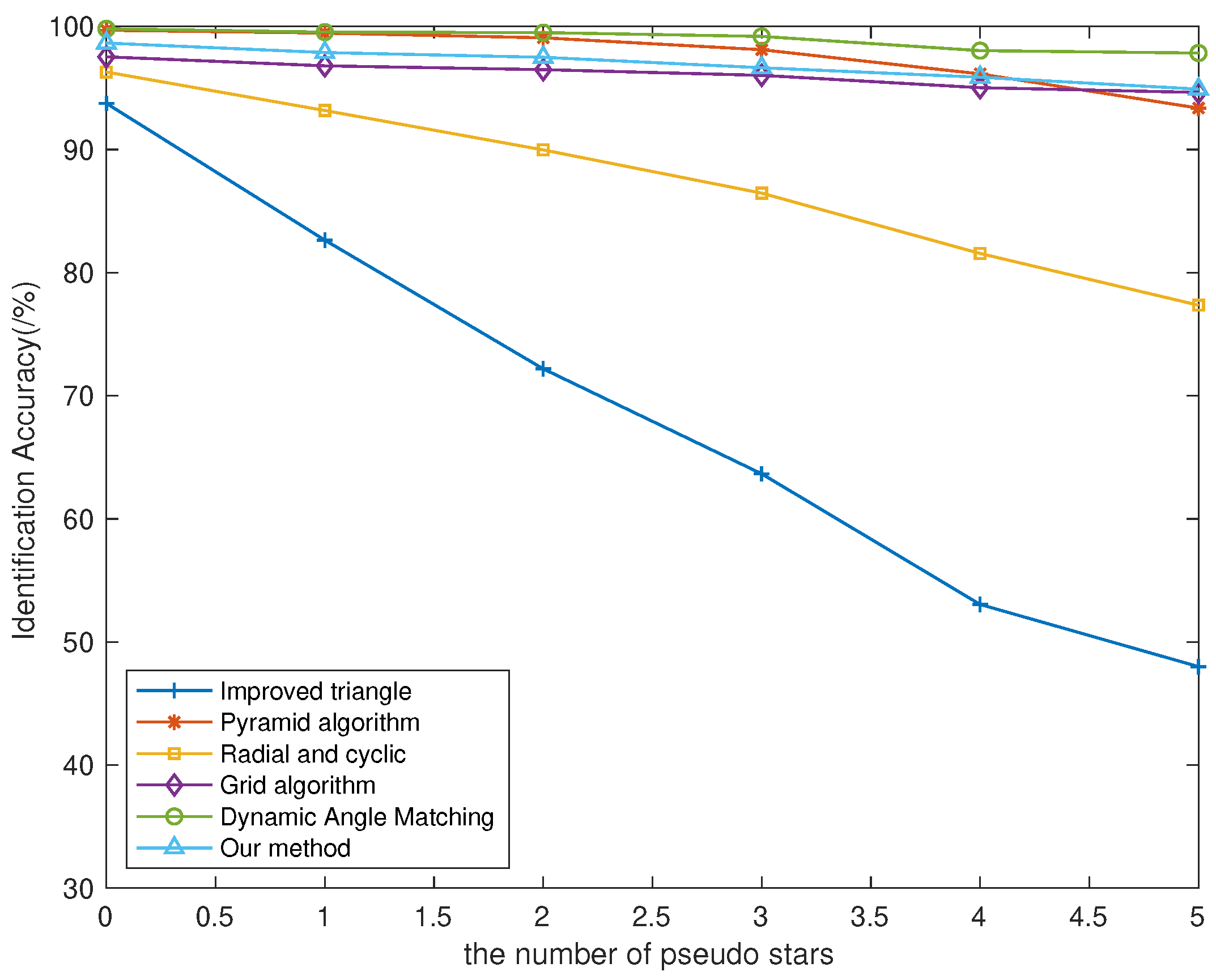
In the simulation of the actual identification process, false star points may occur due to interference from dust and high-energy particles. Therefore, one to five false star points are randomly placed in the simulated star maps to validate the robustness of various star identification algorithms against false star interference. As shown in Figure 9, compared to other identification algorithms, the algorithm based on dynamic angle matching demonstrated the highest recognition rate, while the dynamic distance ratio algorithm’s recognition rate also showed no significant decrease. Even in the presence of five false stars, the algorithm was able to maintain an average recognition rate of $\mathrm{94.91\%}$. Thus, the proposed algorithm demonstrates good robustness against pseudo star interference.

It should be clarified that although in Section 5.2 and Section 5.3 the identification rate of the dynamic angle matching algorithm is comparable to that of the dynamic distance ratio method, there is a significant difference in identification rates between the two in the focal length error and image distortion experiments. This will be discussed in detail in the next section.

5.4. Focal Length Error

In the simulation, the focal length value f is modified to simulate changes in focal length. The accuracy of each identification algorithm is then statistically analyzed under varying focal lengths to assess the robustness of the identification algorithms to focal length changes.

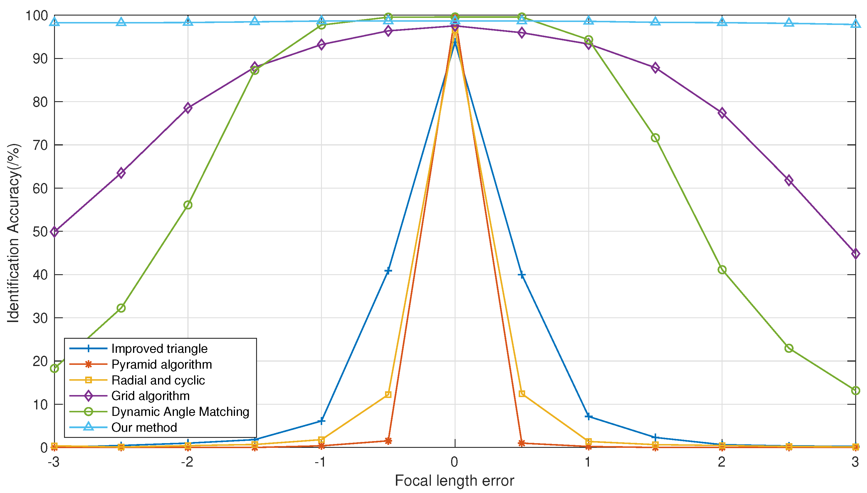
Based on a focal length of $58.4563$ mm, each algorithm’s identification rates are tested with a step of $0.5$ mm, under a range of errors from −3 mm to +3 mm, as shown in Figure 10.

As seen in Figure 10, the proposed identification algorithm, which uses distance ratios as features, demonstrates a clear advantage under focal length errors. Next, a detailed analysis of the impact of focal length variations on each algorithm will be provided.

The improved triangle algorithm and pyramid algorithm, both of which rely on angular distances between stars for identification, show a significant drop in identification rates to below $\mathrm{5\%}$ with slight variations in focal length. Analyzing the reasons behind this reveals that these algorithms depend on the coordinates of the star points in the image coordinate system and the focal length to obtain the direction vectors. Therefore, when there is a deviation between the actual focal length and the set focal length, these algorithms quickly become ineffective.

In the radial axial algorithm, the distances between each neighboring star and the reference star to be identified are measured and used as radial features, with fixed intervals for differentiation. However, as the focal length changes, the positions of the star points also shift, causing variations in the distances between the reference star and its neighboring stars. This ultimately prevents correct radial matching, leading to identification failures. The figure illustrates that as the focal length error increases, the identification rate of this algorithm sharply declines.

The grid algorithm achieves identification by dividing star points into grids. When the focal length changes, the shape of the entire star map also shifts, causing the star points to continue to diverge outward from the field center. When the divergence error of these star points exceeds the interval of each grid in the grid algorithm, effective identification becomes impossible. The figure shows that as the focal length error gradually increases, the identification accuracy of the grid algorithm declines to below $\mathrm{50\%}$.

The distance ratio algorithm is nearly unaffected by changes in focal length, maintaining an identification rate of over $\mathrm{98\%}$. This effectively demonstrates the algorithm’s validity and indicates that it possesses strong robustness in dealing with variations in focal length.

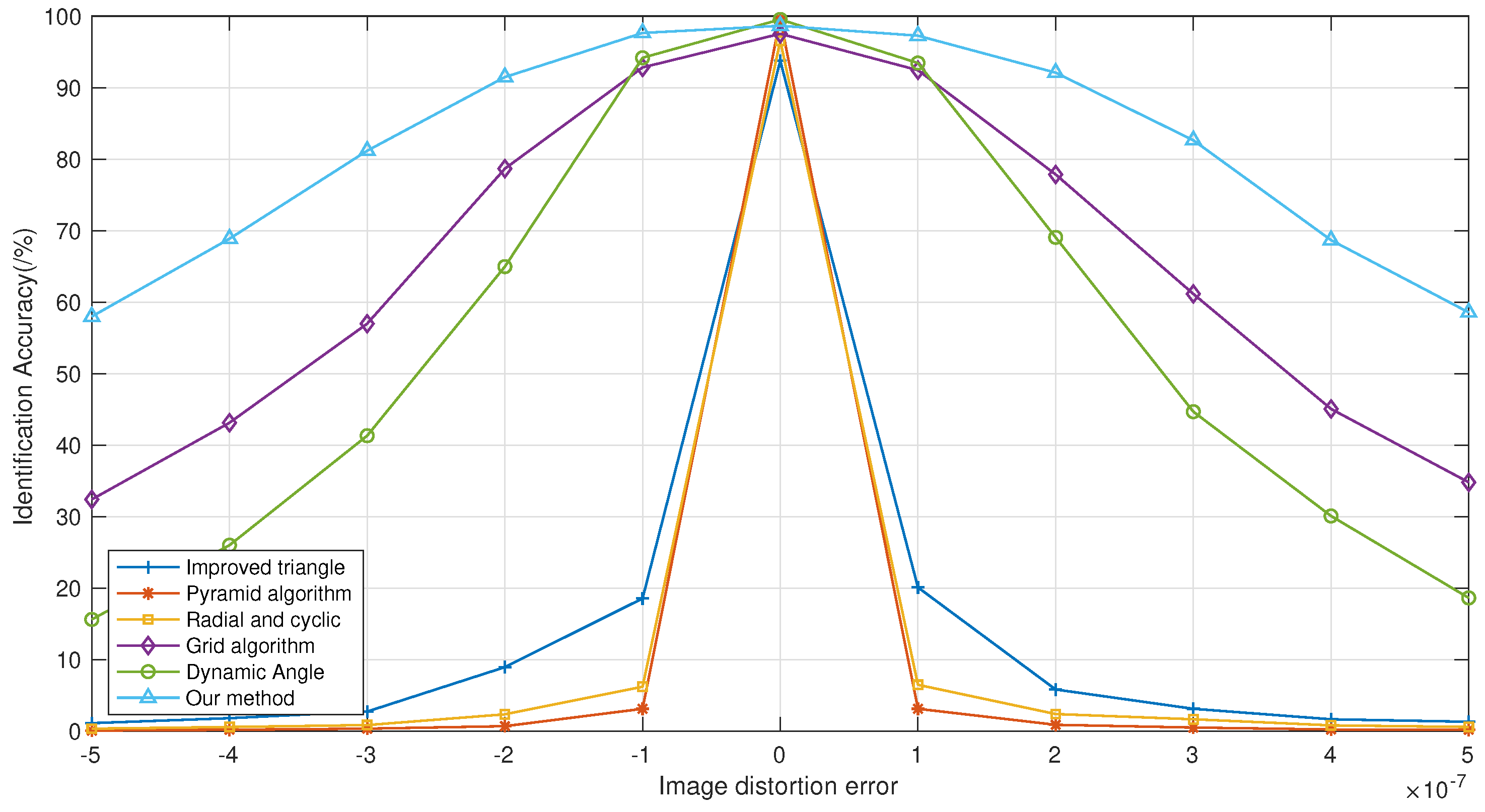
5.5. Image Distortion

By simulating the identification accuracy of various algorithms under radial distortion, we can evaluate their robustness to distortion. We test several values of the distortion coefficient K ranging from $-5\times {10}^{-7}$ to $+5\times {10}^{-7}$ in Equation (14). When the K value is less than zero, it indicates the presence of barrel distortion, while a positive K value signifies the presence of pincushion distortion.

$$\left\{\begin{array}{c}\hfill x_0=x(1+K{r}^2)\\ \hfill y_0=y(1+K{r}^2)\end{array}\right.$$

(14)

As the distortion coefficient increases, the degree of distortion in the star image becomes more pronounced, and the positional deviation of each pixel increases with the distance from the center of the image. When the distortion coefficient is set to 5 × ${10}^{-7}$, the positional deviation reaches 150 pixels at the outermost edge of the image.

From Figure 11, it can be seen that the identification accuracy of all algorithms has decreased. Among them, the grid algorithm, the dynamic angle algorithm from the previous chapter, and the dynamic distance ratio algorithm presented in this section exhibit stronger robustness, especially when the distortion coefficient is small, where the drop in identification accuracy is not significant. Notably, the dynamic distance ratio algorithm shows a clear advantage in tolerance to distortion; while the identification accuracy of other algorithms drops below $\mathrm{30\%}$, this algorithm maintains approximately $\mathrm{60\%}$ accuracy. Therefore, it can be concluded that the algorithm presented in this chapter demonstrates strong robustness against image distortion.

5.6. Comparison of Computation Time

The average computation time of various star identification algorithms was tested using 16,200 simulated star images, and the results are shown in Figure 12.

It can be observed that the proposed algorithm does not demonstrate a significant advantage in computational efficiency compared to other algorithms, particularly when compared to some existing highly efficient algorithms, as there is a gap in computation time. Specifically, we employ a two-dimensional lookup table structure during algorithm execution to optimize search efficiency. The algorithm primarily relies on distance ratios and angular features for matching. Accordingly, the navigation star database is utilized to construct a two-dimensional lookup table by organizing the navigation stars based on distance ratios and angles. The indices of this table are the distance ratios and angles, while the corresponding values represent the relevant navigation star information. This approach enables direct access to navigation stars that meet the requirements during the initial matching phase of dynamic angles, thereby improving the overall search efficiency. Future research will continue to incorporate the characteristics of the navigation star database to construct specific structures, further optimizing the search process and enhancing the execution efficiency of the algorithm.

Nonetheless, computational efficiency is not the primary focus of this study, nor is it the sole criterion for evaluating the algorithm. Instead, the main objective of this research is to enhance the robustness and accuracy of the star identification algorithm under various adverse conditions, particularly in the presence of uncertainties such as image distortion and focal length variations, while maintaining high identification accuracy.

We designed focal length variation experiments and image distortion experiments to evaluate the performance of the proposed algorithm under complex conditions. The experimental results demonstrate that the recognition accuracy of the proposed algorithm is barely affected under these extreme conditions, significantly outperforming traditional algorithms under the same circumstances. Even in cases of severe image distortion or substantial focal length changes, the algorithm is capable of accurately recognizing the targets in star images. This performance advantage enhances the reliability of the algorithm in practical applications, especially when performing star identification tasks in challenging environments, ensuring successful task execution and efficient target identification.

Therefore, although there is some compromise in computational efficiency, the proposed algorithm’s advantages in robustness and accuracy enable it to maintain stable performance in various complex and unpredictable environments. This makes the algorithm particularly suitable for practical tasks with extremely high reliability requirements.

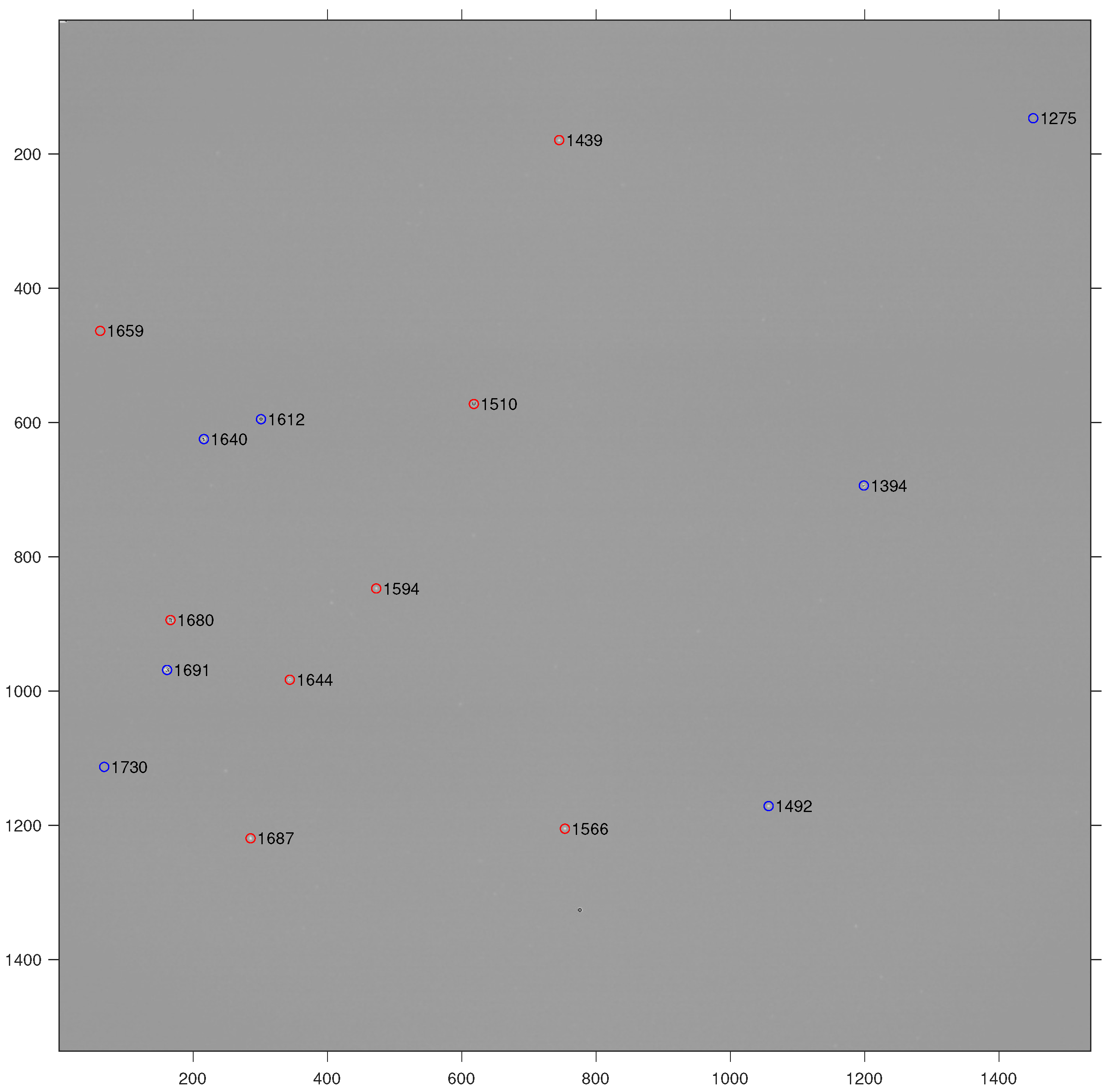
5.7. Replenish Adjacent Stars

Using actual star images for testing, the identification results are shown in Figure 13. Here, the red circles represent successfully recognized stars, while the blue circles indicate stars obtained through the neighbor supplementation algorithm after identification was completed. On the left side of the Figure 14, the star distribution is relatively sparse, providing fewer features, which led to unsuccessful identification when directly applying the identification algorithm. However, with the assistance of the recognized stars, multiple star numbers were further supplemented, thereby increasing the overall number of recognized stars.

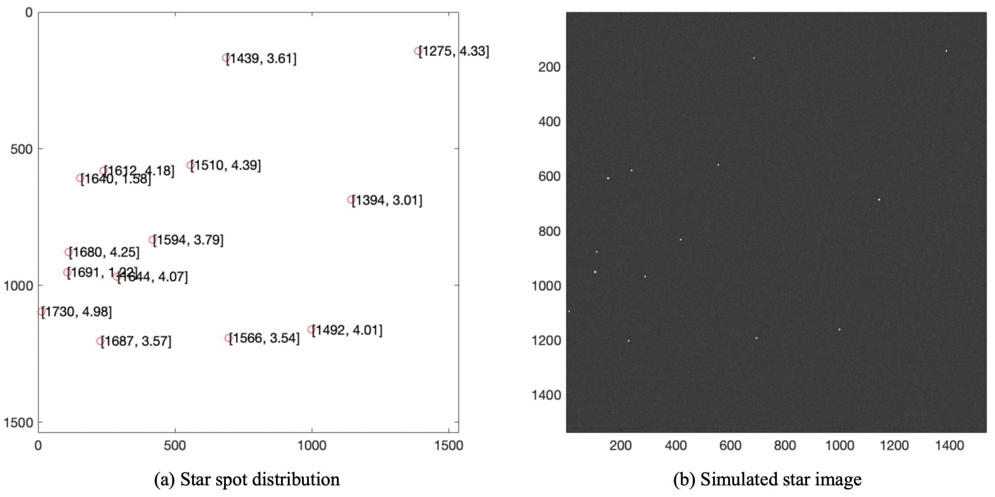
To further verify the reliability of these star identification results, the current attitude of the star sensor is calculated based on these star points, and the simulated star image is presented in Figure 14.

From the simulated star image in Figure 14, it can be observed that the use of the neighbor star supplementation method results in accurate star point identifications, effectively increasing the number of recognized stars. By comparing the relationship between the ideal star point positions and the actual star point positions, this approach provides a possibility of calibrating various parameters of the star sensor. Specifically, the estimated correction for the star image can be made based on the displacement of star point positions, achieving distortion correction.

6. Conclusions

An identification algorithm based on dynamic distance ratios is proposed, transforming previous distance features into ratio-based features to enhance robustness against image distortion and focal length variations. This approach demonstrates strong resilience, especially in the presence of positional noise and false stars. Some pattern matching methods use the nearest neighbor star as a starting point; however, incorrect selection of the starting star can lead to identification failures in cases of significant star extraction errors. To address this issue, the algorithm employs the angles between neighbor stars and the distance ratios between neighbor stars and the observed star as dynamic angular features. These features serve as the starting point for subsequent matching, calculating the matching degree with each navigation star through cumulative angle, and distance verification methods, combined with dynamic ratio calculations. Ultimately, the star with the highest matching degree is identified as the correct navigation star. The algorithm exhibits greater adaptability to distortion, particularly in response to variations in focal length, thereby enhancing its overall robustness.

References

- Yoon, H.; Baeck, K.; Wi, J. Star tracker geometric calibration through full-state estimation including attitude. Int. J. Aeronaut. Space Sci. 2022, 23, 180–191. [Google Scholar] [CrossRef]
- Finney, G.A.; Fox, S.; Nemati, B.; Reardon, P.J. Extremely Accurate Star Tracker for Celestial Navigation. In Proceedings of the Advanced Maui Optical and Space Surveillance (AMOS) Technologies Conference, Maui, HI, USA, 19–22 September 2023; p. 98. [Google Scholar]
- Lu, R.; Zhang, J.; Han, X.; Wu, Y.; Li, L. Dynamic accuracy measurement method for star trackers using a time-synchronized high-accuracy turntable. Appl. Opt. 2024, 63, 3854–3862. [Google Scholar] [CrossRef] [PubMed]
- Bürger, K.C.; Fialho, F.d.O.; Aykroyd, C.R.B. Embedded Star Catalog Calculation Tool for Autonomous Star Trackers; IOP Publishing Ltd.: Bristol, UK, 2024. [Google Scholar]
- Liu, X.; Yan, T.; Zhang, L.; Zhan, H.; Guo, S.; Gao, X.; Xing, F.; You, Z. A Novel Satellite Beacon for Ground-Based All-Day Observation Using a Star Tracker. IEEE Trans. Geosci. Remote Sens. 2024, 62, 5629716. [Google Scholar] [CrossRef]
- Liebe, C.C.; Gromov, K.; Meller, D.M. Toward a stellar gyroscope for spacecraft attitude determination. J. Guid. Control Dyn. 2004, 27, 91–99. [Google Scholar] [CrossRef]
- Mortari, D.; Samaan, M.A.; Bruccoleri, C.; Junkins, J.L. The Pyramid Star Identification Technique. Navigation 2004, 51, 171–183. [Google Scholar] [CrossRef]
- Zhang, G.; Wei, X.; Jiang, J. Star map identification based on a modified triangle algorithm. Acta Aeronaut. Astronaut. Sin. 2006, 27, 1150–1154. [Google Scholar]
- Wei, X.; Zhang, G.; Jiang, J. Star identification algorithm based on log-polar transform. J. Aerosp. Comput. Inf. Commun. 2009, 6, 483–490. [Google Scholar] [CrossRef]
- Padgett, C.; Kreutz-Delgado, K. A grid algorithm for autonomous star identification. IEEE Trans. Aerosp. Electron. Syst. 1997, 33, 202–213. [Google Scholar] [CrossRef]
- Na, M.; Zheng, D.; Jia, P. Modified grid algorithm for noisy all-sky autonomous star identification. IEEE Trans. Aerosp. Electron. Syst. 2009, 45, 516–522. [Google Scholar] [CrossRef]
- Silani, E.; Lovera, M. Star identification algorithms: Novel approach & comparison study. IEEE Trans. Aerosp. Electron. Syst. 2006, 42, 1275–1288. [Google Scholar]
- Zhang, G.; Wei, X.; Jiang, J. Full-sky autonomous star identification based on radial and cyclic features of star pattern. Image Vis. Comput. 2008, 26, 891–897. [Google Scholar] [CrossRef]
- Wei, X.; Wen, D.; Song, Z.; Xi, J.; Zhang, W.; Liu, G.; Li, Z. A star identification algorithm based on radial and dynamic cyclic features of star pattern. Adv. Space Res. 2019, 63, 2245–2259. [Google Scholar] [CrossRef]
- Mehta, D.S.; Chen, S.; Low, K.S. A rotation-invariant additive vector sequence based star pattern identification. IEEE Trans. Aerosp. Electron. Syst. 2018, 55, 689–705. [Google Scholar] [CrossRef]
- Li, J.; Wei, X.; Zhang, G. Iterative algorithm for autonomous star identification. IEEE Trans. Aerosp. Electron. Syst. 2015, 51, 536–547. [Google Scholar] [CrossRef]
- Shi, C.; Zhang, R.; Yu, Y.; Lin, X. On-Orbit Geometric Distortion Correction on Star Images through 2D Legendre Neural Network. Remote Sens. 2022, 14, 2814. [Google Scholar] [CrossRef]
- Oudmaijer, R.D.; Van der Veen, W.; Waters, L.; Trams, N.; Waelkens, C.; Engelsman, E. SAO stars with infrared excess in the IRAS Point Source Catalog. Astron. Astrophys. Suppl. Ser. 1992, 96, 625–643. [Google Scholar]
- Sun, X.; Zhang, R.; Shi, C.; Lin, X. Star Identification Algorithm Based-on Dynamic Angle Matching. Acta Opt. Sin. 2021, 41, 1610001. [Google Scholar]