Article

RS-FeatFuseNet: An Integrated Remote Sensing Object Detection Model with Enhanced Feature Extraction

1
National Laboratory on Adaptive Optics, Chengdu 610209, China
2
University of Chinese Academy of Sciences, Beijing 101408, China
3
Institute of Optics and Electronics, Chinese Academy of Sciences, Chengdu 610209, China
*
Author to whom correspondence should be addressed.
Remote Sens. 2025, 17(1), 61; https://doi.org/10.3390/rs17010061
Submission received: 5 October 2024 / Revised: 18 December 2024 / Accepted: 24 December 2024 / Published: 27 December 2024
(This article belongs to the Special Issue Advanced AI Technology in Remote Sensing)

Abstract

:
With the advancement of satellite and sensor technologies, remote sensing images are playing crucial roles in both civilian and military domains. This paper addresses challenges such as complex backgrounds and scale variations in remote sensing images by proposing a novel attention mechanism called ESHA. This mechanism effectively integrates multi-scale feature information and introduces a multi-head self-attention (MHSA) to better capture contextual information surrounding objects, enhancing the model’s ability to perceive complex scenes. Additionally, we optimized the C2f module of YOLOv8, which enhances the model’s representational capacity by introducing a parallel multi-branch structure to learn features at different levels, resolving feature scarcity issues. During training, we utilized focal loss to handle the issue of imbalanced target class distributions in remote sensing datasets, improving the detection accuracy of challenging objects. The final network model achieved training accuracies of 89.1%, 91.6%, and 73.2% on the DIOR, NWPU VHR-10, and VEDAI datasets, respectively.

1. Introduction

As more satellites are deployed and diverse imaging sensors are developed, remote sensing images are generated in huge quantities [1]. These images are pivotal in resource exploration, disaster detection, military analysis, air quality monitoring, etc. Effectively processing these remote sensing images stands as a prominent research focus. Identifying objects of interest within images automatically is a fundamental objective in remote sensing image processing, which is known as remote sensing image object detection [2,3].
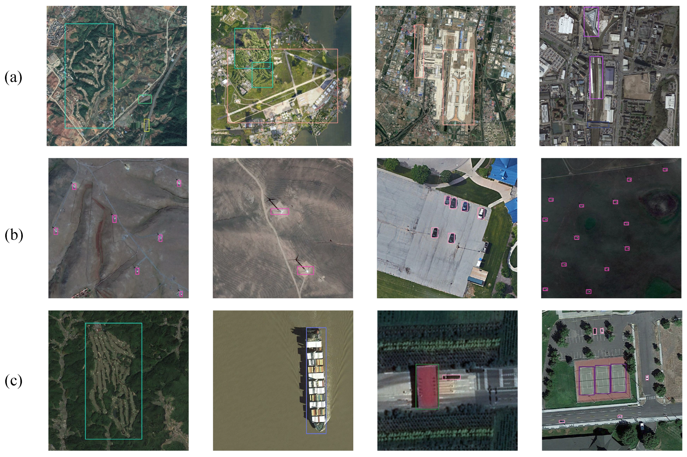
In this study, our research focuses on visible spectral remote sensing images. Most traditional methods rely on hand-designed features for designing classifiers [4]. These methods usually involve a sequence of steps including region proposal, feature extraction, feature fusion, and classifier training. While these methods laid the foundation for object detection, they proved to be less efficient, less adaptable, and unsuitable for the high-resolution, multi-directional, and object-dense nature of remote sensing objects [5,6]. Object detection algorithms leveraging deep learning outperform traditional approaches that necessitate handcrafted features by directly using networks for end-to-end detection, resulting in higher accuracy and detection efficiency. ParNet [7] increases the receptive field without affecting the depth by constructing the Skip–Squeeze–Excitation (SSE) branch, which helps to extract features. However, remote sensing detection still encounters several challenges. In Figure 1, we present a selection of representative visible spectral remote sensing images.
At present, remote sensing object detection algorithms typically encounter the following challenges:
(1) Remote sensing systems encounter issues such as atmospheric interference, uncontrollable observation conditions, and complex imaging scenes, leading to complex backgrounds in remote sensing images. Most existing methods focus on extracting more effective features from objects [8] while overlooking the learning of contextual relationships. Some existing networks based on Transformer for learning contextual relationships often introduce significant increases in computational complexity and consume a large amount of computational resources [9]. (2) Remote sensing images exhibit large-scale differences and often contain numerous small objects. Small objects, due to their limited size, suffer from insufficient features that can affect detection accuracy. (3) Different types of objects exist in remote sensing datasets with significant variations in the numbers of different categories of objects. This unbalanced distribution can lead to inadequate learning for minority classes, affecting the model’s performance.
The principal achievements of this study are as follows. (1) Efficient Multi-Scales and Multi-Head Attention (ESHA): We proposed an attention mechanism called ESHA. By integrating multi-head self-attention (MHSA) to extract global features, this module not only better captures the relationships between objects and backgrounds, providing more comprehensive attention at different scales, but also helps the model understand the positions and features of objects in complex backgrounds. This further optimizes the utilization of contextual information, enhances the model’s perception of complex scenes, and enables better adaptation to remote sensing images of varying scales and complexities. (2) Parallel Feature Enhancement Module (PFEM): Drawing inspiration from the ParNet network, we design a new feature enhancement module named PFEM to enhance feature extraction capabilities. This module, without increasing network depth, improves the network’s ability to extract and fuse features, effectively enhancing localization accuracy. (3) An Integrated Remote Sensing Object Detection Model with Enhanced Feature Extraction (RS-FeatFuseNet): This study introduces an improved YOLOv8, named RS-FeatFuseNet, which incorporates attention mechanisms and enhances feature extraction and fusion components. Furthermore, we improve the existing loss function with focal loss to focus on that are difficult to classify, thus improving the effectiveness of learning on these objects.

2. Related Works

The current mainstream deep learning-based detection algorithms can be grouped into the following three types: two-stage detection algorithms, one-stage detection algorithms, and Transformer-based detection algorithms. The two-stage detection algorithm represented by the R-CNN series was introduced by Girshick [8,10,11,12,13], which first generates candidate frames for objects in the image. The second category bypasses the generation of region proposals and performs object classification and regression directly within the network. Transformer-based detection algorithms, which were popularized in Natural Language Processing (NLP) in 2017 [14], and the Vision Transformer (ViT) [15], establish global self-attention across the entire image, pioneering the fusion of Transformers and CNNs in detection tasks.

2.1. Two-Stage Detection Algorithms

He et al. [16] addressed the limitation of fixed input image size by introducing a spatial pyramid pooling. Fast R-CNN [11] employs a pooling layer to scale candidate boxes and utilizes a feature sharing mechanism for extracting features. Faster R-CNN [12] proposes the use of candidate networks instead of search algorithms as in R-CNN, which significantly reduces the time and resources consumed during the search for candidate region proposals. Weng et al. introduce a rotating object detection method [17] to tackle the challenge posed by the random orientation of remote sensing objects. Yan [18] employed attention mechanisms to enhance the Feature Pyramid Network (FPN) and extract pertinent information regarding tailings ponds. Yin [19] applies multi-scale training to Fast R-CNN to improve the network’s robustness. Wang [20] proposed a method that performs inference directly on a large amount of data without requiring any annotations. Peng [21] introduced a weighted label smoothing (WLS) loss that can account for the similarity between different clustered samples. Ren [22] incorporates contextual information to further improve the accuracy. EfficientDet’s [23] proposed feature pyramid structure, BiFPN, better integrates features of different scales through cross-layer connections. In 2023, Wang et al. introduced RegNet [24], which automatically seeks the optimal network sampling path to address the issue of information loss due to sampling. Bashir et al. [25] proposed a super-resolution-based GAN method that utilizes residual feature aggregation to enhance image quality, thereby improving small object detection accuracy. Liu et al. [26] presented the scene-relevant SRAF-Net network, which acquires contextual scene information around objects from a scene-enhancement perspective.

2.2. One-Stage Detection Algorithms

One-stage algorithms are faster while ensuring detection accuracy. The most popular one-stage algorithms are YOLO series [27,28,29,30,31,32], SSD [33] and the RetinaNet series [34]. For the characteristics of remote sensing objects, Lang designs a plug-in-play module that fuses Convolution and Transformer [35]. Huo et al. proposed an attention module and utilized CSP-PAN as a neck detection network [36]. So far, the YOLO family is a collection that encompasses YOLOv1 [27]-YOLOv10 [32] and other variants. They are widely used in academia and industry, and they gained significant traction in the remote sensing detection. TPH-YOLO [9] is designed with a Transformer detector head to replace the original detector head and incorporates the CBAM [37] attention mechanism to recognize dense objects and improve detection accuracy. FFCA-YOLO [38] improves the accuracy of small object recognition by designing a spatial context-aware module (SCAM) and a feature enhancement module FEM. CA-YOLO [39] utilizes the coordinate attention to establish dependency among pixels, which is effective in suppressing redundant backgrounds. Lai et al. devised a feature extraction module that merges a CNN with multi-head attention to broaden the receptive field [40]. In summary, YOLO not only has high accuracy and speed but also has good scalability, so we selected YOLO as the baseline network. SSD [33] introduced multi-scale feature maps to detect objects of various scales using features from different levels, enhancing the detection capability. However, SSD did not address the issue of foreground–background class imbalance. Lin et al. proposed a detection algorithm, RetinaNet [41], which leverages F o c a l _ L o s s to tackle the problem of foreground–background class imbalance with some success. CornerNet [42] innovatively utilizes object corner information for object detection instead of traditional bounding boxes. FMSSD [43] designed a spatial pyramid based on parallel expanding convolutional layers to enlarge the receptive field, but excessive enlargement of the receptive field may lead to shallow information loss.

2.3. Transformer-Based Algorithms

Swin-Transformer [44] was developed to enable information interaction between different image tokens through window cyclic offset. CSWin Transformer [45] designed a method that can compute attention in two dimensions, which not only expands the local receptive field but also reduces complexity. Wang, et al. [46] proposed a new method to embed CNN features into ViT. This enhancement allows for the extraction and merging of global and local information, thereby bolstering ViT’s classification capability. In addition, TPH-YOLO [9] and the network [47] are both explorations of the role of Transformer within the realm of remote sensing. Transformer primarily consists of multi-head attention. The unique ability of multi-head attention to focus on different aspects of the input data simultaneously and capture complex relationships implies the potential value of exploring its application. It can potentially enhance the model’s performance by better understanding and processing the relationships between different elements in the data, especially in tasks such as object detection and classification where understanding the context and global structure is crucial.

3. Materials and Methods

3.1. RS-FeatFuseNet

As shown in Figure 2, YOLOv8’s backbone section serves as the main network for feature extraction. The neck section is in charge of fusing and optimizing the features extracted by the backbone while also playing a dual role in feature extraction and enhancement. The head section utilizes the feature information extracted in the preceding steps to predict the class and location of objects.
We made three main enhancements to the YOLOv8 model. First of all, we introduced the ESHA module before the large detection head. The large detection head typically handles larger-scale objects, and introducing this module at this stage helps the model better understand semantic information in the images, enhancing its perception of global information. We replaced Conv module in the C2f part of the neck section with the Parallel Feature Enhancement Module (PFEM) to create a new C2f, enhancing feature extraction and fusion capabilities. Additionally, we improved the loss function to make the model pay more attention to objects that are harder to detect, thus increasing the detection accuracy.
Table 1 shows the structure of our RS-FeatFuseNet. The ‘Index’ is used to uniquely identify each layer in the neural network structure, providing a clear identification of the network’s hierarchical layout. The ‘Module’ indicates the specific module employed by each layer, aiding in understanding the function and purpose of each layer. ‘From’ displays the input source for each layer, where −1 signifies that the layer directly receives the output from the previous layer. N is used to denote the number of repeated modules. The ‘Argvs’ column contains lists of different parameters with specific meanings depending on each module type: ‘Conv’ layers include the input channel number, output channel number, kernel size, and stride. Only the fourth item of the ‘C2f’ layer is different from that of the ‘Conv’ layer, and it represents whether bias is used (‘True’ indicates the use of bias); SPPF layers include the input channel number, output channel number, and pool size; ‘Upsample’ layers include ‘None’ (it indicates no additional input is required), the upsampling factor, and the upsampling method (e.g., ‘nearest’); ‘Concat’ layers comprise a list of connected layer indices; the ‘Improved_C2f’ layer is the same as the ‘C2f’ layer except that the former does not have the fourth item; ‘ESHA’ layers include the input channel number and output channel number; ‘Detect’ layers include lists of input feature map indices and output channel numbers. ‘Parameters’ represent the number of parameters for each layer.

3.2. Efficient Multi-Scales and Multi-Head Attention

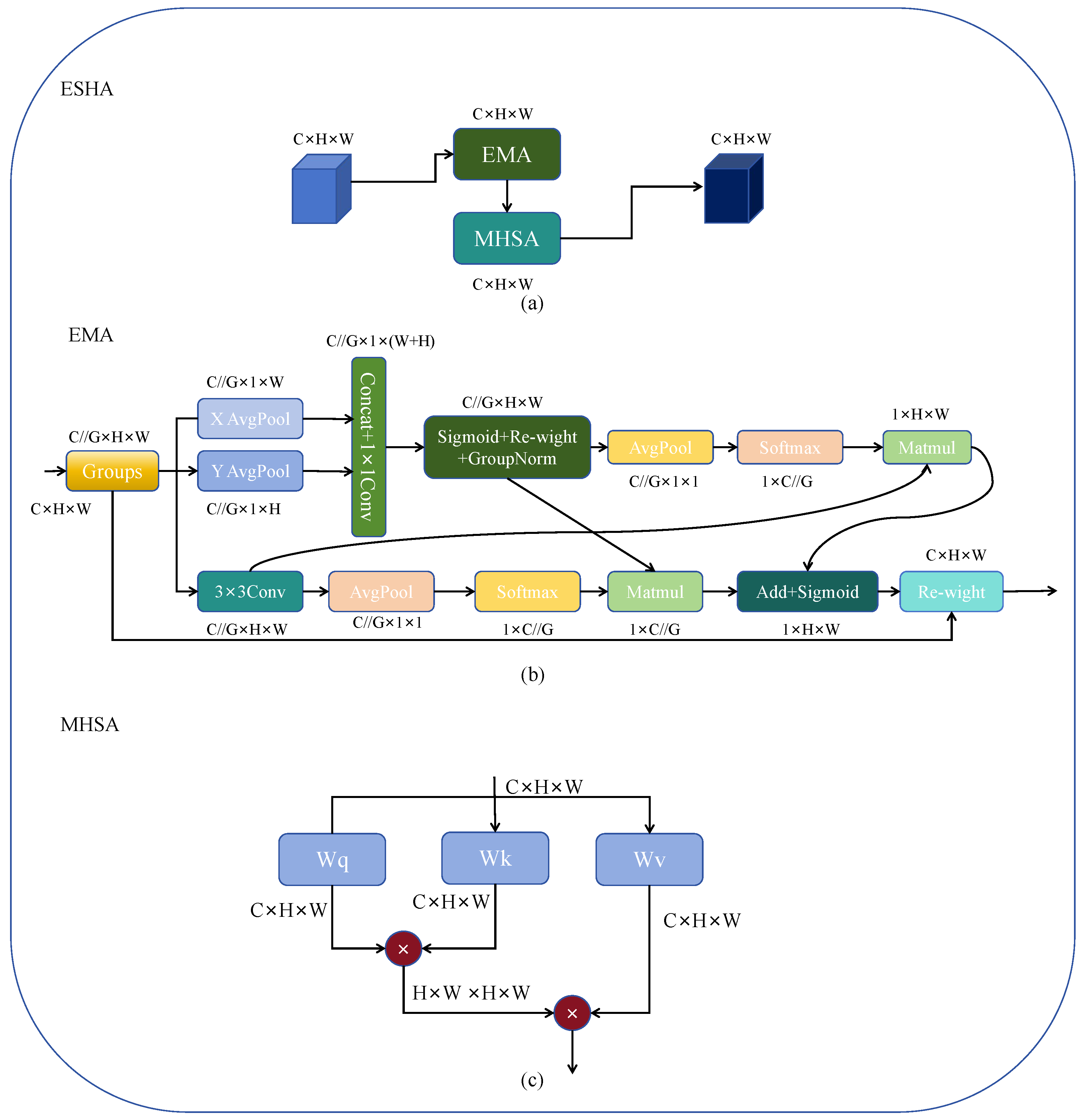
Remote sensing images often contain complex backgrounds and varied scales. Compared to natural images, a remote sensing image demands more detailed information to exclude noise interference and concurrently requires a larger receptive field to assist in detection. A detector relying solely on a CNN architecture would struggle to extract global information effectively due to the constraints of kernel size. To address this issue, we developed the ESHA module, as illustrated in Figure 3a. The module employs Efficient Multi-Scale Attention Module with Cross-Spatial Learning (EMA) [8] as a cross-space multi-scale attention mechanism for initial local multi-scale attention extraction. The cross-spatial learning and multi-scale attention in the EMA module enable it to achieve good detection performance of different scales. It then integrates an enhanced MHSA to extract global features.
The structure of EMA is depicted in Figure 3b. EMA processes input feature maps using 1 × 1 and 3 × 3 branches in parallel. The 1 × 1 branch conducts global average pooling along the horizontal and vertical dimensions, which is followed by ‘Concat’ and channel adjustment through 1 × 1 C o n v . The output is subjected to non-linear transformation using the ‘Sigmoid’ and channel fusion via Re-weight to facilitate information exchange between these two 1 × 1 branches. On the other hand, the 3 × 3 branch employs 3 × 3 ‘Conv’ to facilitate local cross-channel interactions, thereby expanding the feature space. Subsequently, the re-weighted results from the 1 × 1 branch are subjected to GroupNorm, and the output conducts global average pooling and is processed through the ‘Softmax’ with the output of the 3 × 3 branch. The processed outputs of the 1 × 1 and 3 × 3 branches and the original 3 × 3 and 1 × 1 branches are subjected to ‘Matmul’ to achieve cross-space learning and fusion. Additionally, the branches of different scales excel in detecting objects of varied scales. By applying attention maps to the input features, the module ultimately achieves cross-space multi-scale feature attention extraction. Combining the two outputs further enhances feature information, followed by fitting through the ‘Sigmoid’, and ultimately re-weighting via the re-weight function to achieve cross-space multi-scale attention feature extraction.
After the EMA module, we added an MHSA to capture contextual information around the targets, aiding the model in further understanding the relationship between targets and backgrounds. In complex scenarios, MHSA can model spatial relationships between targets, assisting the model in better comprehending interactions and positional relationships among targets. It also possesses a degree of adaptability and flexibility, allowing for dynamic adjustments based on the characteristics of different scenes and targets, thereby accommodating detection requirements in diverse scenarios. Unlike the MHSA in the Transformer, since the position is already encoded in the EMA module, we delete the position information and remove the layer norm, dropout and Gelu operations in the MHSA in order to minimize computational demands.
We employ the feature map directly as input for self-attention, eliminating the embedding operation. The simplified multi-head self-attention module is depicted in Figure 3c.
Its formula is represented by Equation (1).
Q , K , V = L i n e a r ( x ) Q i , K i , V i = G r o u p s ( Q , K , V ) , i = 1 h A t t e n t i o n ( Q i , K i , V i ) = s o f t m a x ( Q i K i T / c k 0.5 ) V i A t t e n t i o n ( Q , K , V ) = C o n c a t ( A t t e n t i o n ( Q i , K i , V i ) ) O u t p u t = ( A t t e n t i o n ( Q , K , V ) ) W o
where x represents input features, while Q, K, and V denote the linear transformations of x. G r o u p s signifies the grouping operation, h represents the number of attention heads, and Q i , K i , and V i refer to the Q, K, V values of the ith attention head. The term s o f t m a x denotes the softmax function, and C o n c a t denotes the concatenation operation. c k represents the feature dimension of K i . The martix W o symbolizes the output transformation matrix for mapping linear vectors back to the feature space. o u t p u t represents the ultimate result or final output.

3.3. Parallel Feature Enhance Module

Remote sensing objects are typically smaller in scale and may have fewer distinguishable features. This necessitates more effective feature extraction and fusion modules to ensure accurate detection in remote sensing applications. While the C2f module functions as a critical feature fusion element within YOLOv8, specifically crafted to amalgamate feature maps from different scales, it may not suffice for detecting small objects in remote sensing images due to its limitations in feature extraction. Figure 4 illustrates the C2f structure of YOLOv8. The input feature map is transformed via the initial CBS, generating an intermediate feature map. Subsequently, this map is then split into two parts: one part is inputted into a series of consecutive bottleneck modules for processing, while the other part of the feature map is concatenated in the Concat module, forming a fused feature map. The concatenated feature map then undergoes processing through the second convolutional layer to obtain the ultimate output feature map.
We have primarily improved the bottleneck section in C2f. As illustrated in Figure 5a, we substituted the first part of the bottleneck with the Parallel Feature Enhancement Module (PFEM). The detailed structure of the PFEM is shown in Figure 5b. This design enables the network to extract diverse and rich features from different paths simultaneously. By integrating and enhancing features through operations like ‘Sigmoid’ for feature integration and adjustment, coupled with the ‘SiLU’ for refinement and enhancement, the network effectively captures and represents critical information in the data. This process enhances the network’s feature representation capability and learning effectiveness, leading to improved object recognition and localization in object detection tasks. Initially, 1 × 1 convolutions and 3 × 3 convolutions are employed to extract two different scales and complexities of information from the original features. The original features are then subjected to average pooling, max pooling operations, and the ‘Sigmoid’ function to learn feature importance. The output is multiplied with the original features to enhance the features. Subsequently, different levels of feature information are fused to acquire a more diverse third feature representation. The three types of features are element-wise added to achieve fusion of different kinds of features, enhancing feature diversity and representational capacity. Finally, the integrated features undergo non-linear transformation via the ‘SiLU’ activation function to enhance their representational capacity. Equation (2) demonstrates the calculation process of the PFEM.
x 1 = B N [ f 1 × 1 ( x ) ] x 2 = B N [ f 3 × 3 ( x ) ] x 3 _ 1 = A v g P o o l [ B N ( x ) ] x 3 _ 2 = M a x P o o l [ B N ( x ) ] x 3 = S i g m o i d [ f 1 × 1 ( x 3 _ 1 + x 3 _ 2 ) ] + x X o u t p u t = S i L U ( x 1 + x 2 + x 3 )
where x represents the input, f 1 × 1 represents the 1 × 1 convolution; similarly, f 3 × 3 represents the 3 × 3 convolution. A v g P o o l represent the global average pooling, and the M a x p o o l denotes global maximum pooling operations. The S i L U activation function is used for processing. X o u t p u t is the final output.

3.4. Loss Function

The training process involves comparing ground truth with predicted results and optimizing them by adjusting the network parameters through gradient backpropagation. The loss function of YOLOv8 consists of two parts: classification loss and regression loss.
To determine the detected category and produce the confidence output, the classification loss function utilizes VFL loss. For multiple classifications, the formula is Equation (3).
L = 1 N i L i = 1 N i c = 1 M y i c l o g ( p i c ) , i = 1 N
i represents the ith detection object, varying from 1 to N, where N stands for the total number of detection objects. M indicates the number of categories. y i c takes binary values of 0 or 1, with 1 indicating the true category of sample i as c and 0 otherwise. p i c represents the predicted probability that observation sample i belongs to category c.
In regression scenarios, the regression loss is employed to measure the degree of intersection between bounding boxes. This measure usually involves comparing the regression of boxes by comparing the ratio of the object box to the predicted box.
The principle of IoU is depicted in Figure 6 to visually illustrate this concept.
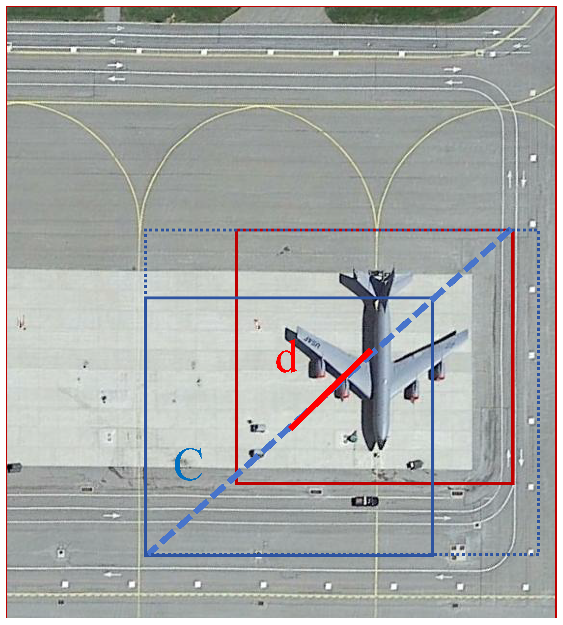
In contrast to IoU, C I o U additionally incorporates the distance between the centroids of the actual and predicted boxes (denoted as ‘d’) and the diagonal distance between the minimum enclosing rectangles of the two boxes (indicated as ‘c’ in Figure 7).
For instance, in scenarios where two boxes exhibit no overlap, resulting in an IoU value of 0, a traditional IoU may hinder backpropagation. C I o U serves as an effective solution to this challenge by considering additional spatial information, thereby facilitating robust optimization even in cases of non-overlapping boxes.
The specific formula for C I o U is Equation (4):
C I o U = I o U ρ 2 ( b , b g t ) c 2 α υ υ = 4 π 2 ( a r c t a n ( w g t h g t ) a r c t a n ( w h ) ) 2 α = υ ( 1 I o U ) + υ
The Complete Intersection over Union ( C I o U ) formula assesses the similarity between two bounding boxes. It comprises the Intersection over Union ( I o U ) term, representing the overlap between these boxes, adjusted by the term ρ 2 ( b , b g t ) c 2 , where ρ 2 ( b , b g t ) denotes the Euclidean distance between the centers of the predicted bounding box b and the ground truth bounding box b g t , and c denotes the diagonal length of the bounding boxes. Additionally, υ is employed to assess aspect ratio’s consistency between the predicted bounding box dimensions w and h and the ground truth dimensions w g t and h g t . The coefficient α modulates the influence of the aspect ratio term relative to the I o U term within the C I o U computation.
However, a notable issue with C I o U is its limited ability to effectively balance the difficulty levels of samples within detection boxes. Therefore, we introduce F o c a l _ L o s s to enhance C I o U . F o c a l _ L o s s represents an enhanced variant the cross-entropy loss function, which is designed to hadle class imbalances in binary classification problems, with its formulation illustrated in Equation (5).
L F L = y ( 1 p ) γ l o g ( p ) ( 1 y ) p γ l o g ( 1 p )
In this loss function, L F L represents the F o c a l _ L o s s function tailored to mitigate class imbalance challenges, where y signifies the true label of a sample, p denotes the model’s predicted probability for that class, and γ acts as a parameter modulating the impact of the focusing mechanism. The terms ( 1 p ) γ and p γ dynamically adjust the loss computation by de-emphasizing well-classified instances and amplifying the contribution of challenging samples, thus enhancing the model’s focus on harder-to-classify examples.
FocalL1 loss is inspired by the concept of F o c a l _ L o s s but is tailored to address imbalances in regression tasks. In the domin of object detection, we regard the disparity between high and low-quality samples as a significant factor affecting model convergence. In object detection scenarios, a majority of predicted boxes derived from anchor points exhibit relatively low I o U with the ground truth, categorizing them as low-quality samples. Training on these low-quality samples can result in significant fluctuations in loss. FocalL1 aims to solve the class imbalance issue between high and low-quality samples.
In this study, By introducing the idea of F o c a l _ L o s s , we use the adjustment factor gamma to adjust the loss weights, and thus obtain a new loss function named F o c a l _ C I o U , which is represented as Equation (6).
F o c a l _ C I o U = ( 1 I o U ) γ C I o U
The formula combines the metrics I o U and C I o U . By raising the value of I o U to the power of γ and multiplying it with C I o U , the formula adjusts the weight of C I o U to be influenced by I o U , providing a more nuanced assessment of the similarity between two bounding boxes in object detection tasks. The parameter γ serves as a tuning factor that controls the influence of the I o U and C I o U metric. A higher value of γ will amplify the effect of I o U on the final metric, while a lower value will reduce its impact. This formulation helps to more comprehensively consider two different evaluation metrics when evaluating the performance of object detection algorithms.
3.5. Experimental Platform and Evaluation Metrics

3.5.1. Experimental Platform

Experimental platform and configuration of the experimental environment are as shown in Table 2.

3.5.2. Evaluation Metrics

We employ precision, recall, average precision (AP), mean average precision (mAP) and GFLOPs as evaluation metrics, which are commonly utilized in object detection. Except for GFLOPS, the others are standard accuracy metrics, where higher values indicate greater model precision. Conversely, a lower GFLOPs value denotes reduced computational resource consumption.
R e c a l l = T P T P + F N P r e c i s i o n = T P T P + F P
In Equation (7), a sample with a confidence level surpassing the threshold and the predicted type matching the labeled type is denoted as a True Positive ( T P ). False Positives ( F P ) represent the instances where the model erroneously identifies background or non-object regions as object regions. On the other hand, if the model incorrectly classifies a positive sample as a negative sample, it is categorized as a False Negative ( F N ). R e c a l l quantifies the number of positive samples correctly detected by the model, while p r e c i s i o n measures how many samples identified as positive are indeed positive. The calculation is Equation (8).
A P = 0 1 P ( R ) d ( R ) m A P = 1 c l a s s e s 0 1 P ( R ) d ( R )
By plotting precision–recall (PR) curves, the A P (average precision) value for each category can be determined by calculating the area under the PR curve. Consequently, m A P is obtained by averaging the A P values. The formulas are described in Equation (8).
GFLOPs are computed based on the count of floating-point operations with higher values indicating a more computationally demanding network.

4. Results

4.1. Dataset

Experiments were conducted using both the DIOR dataset [48], the NWPU VHR-10 dataset [49] and the VEDAI dataset [50]. We will validate the effectiveness of our network models and modules on these two datasets, respectively.

4.1.1. DIOR

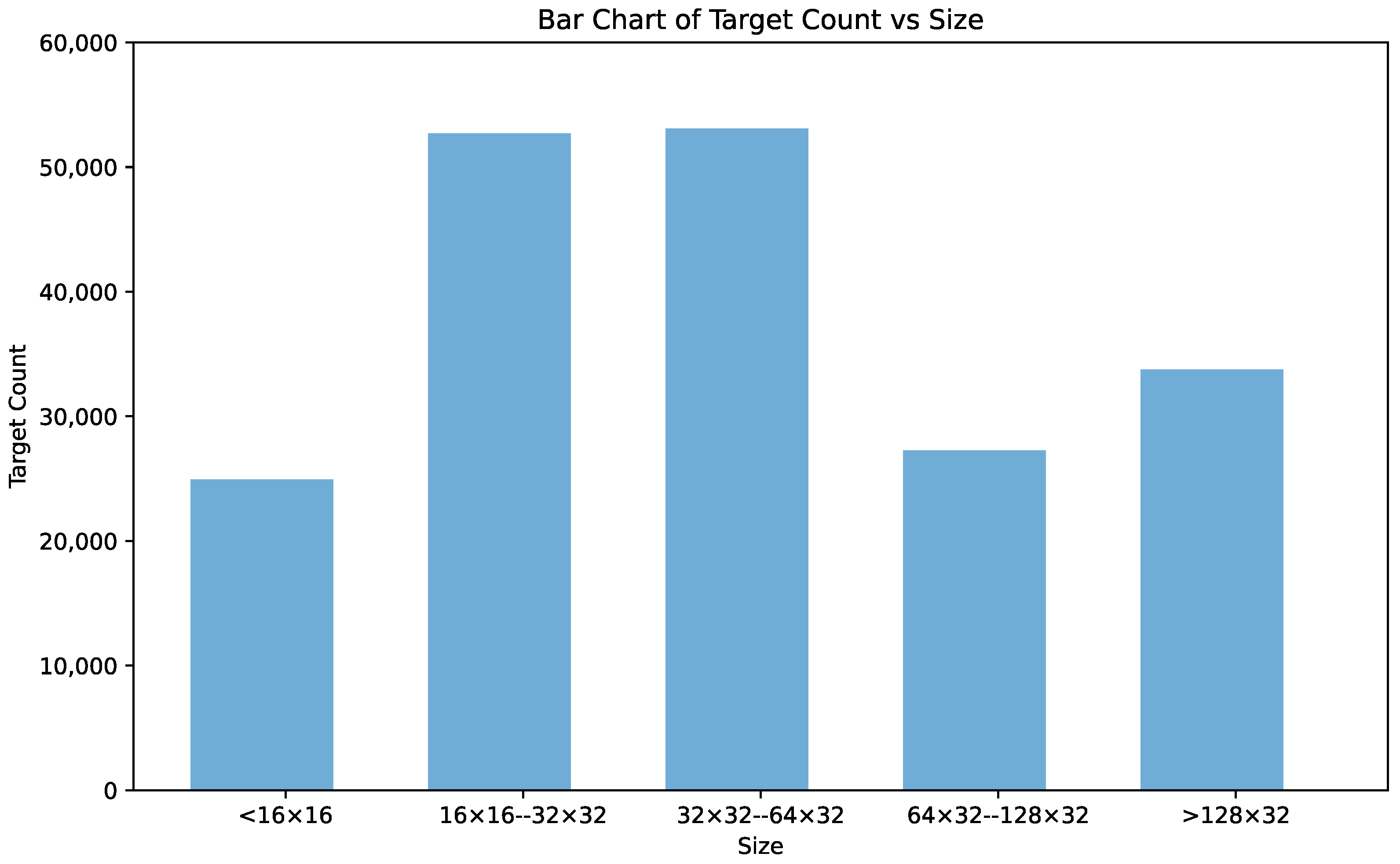
We conducted comprehensive experiments on the DIOR dataset. The DIOR dataset is a diverse collection of optical remote sensing objects, including 20 object classes such as chimneys, dams, and bars [48]. The images in this dataset are sized at 800 × 800 pixels, covering various scales of objects. This diversity in object scales poses significant challenges for object detection. The size ranges within the DIOR dataset are shown in Figure 8.
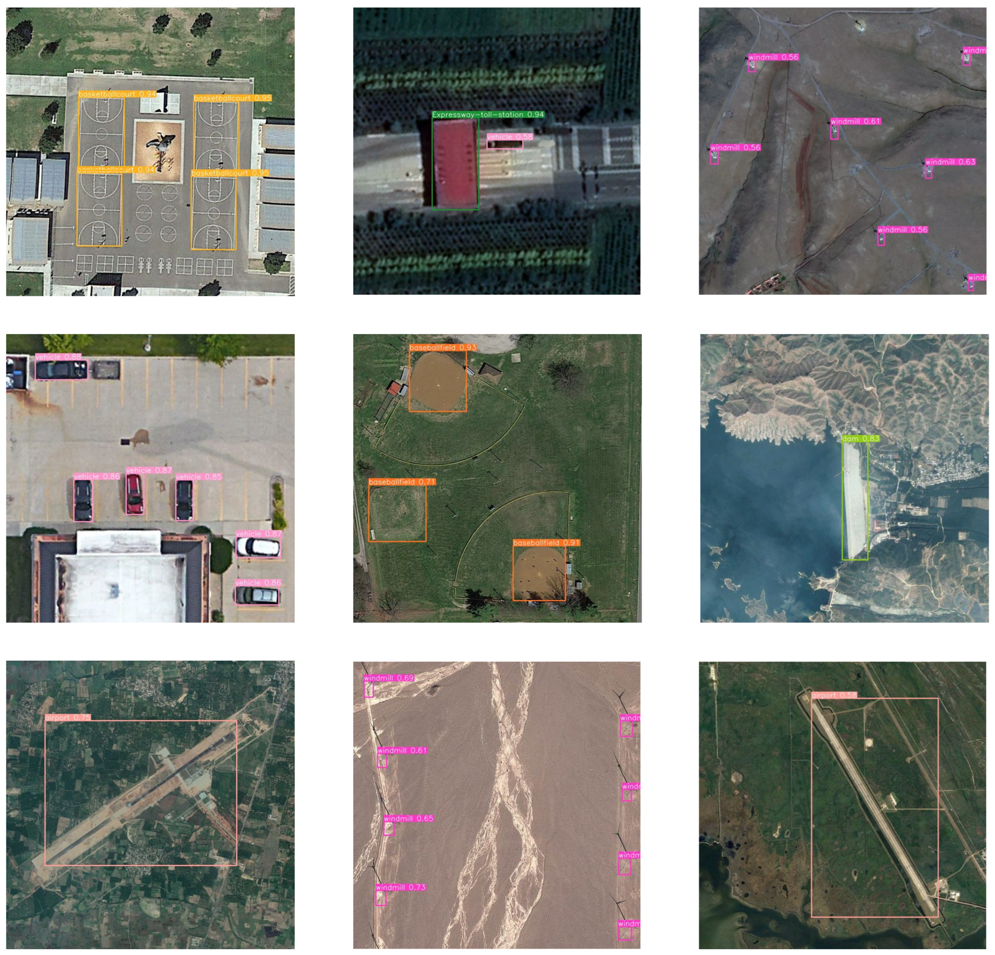
Figure 9 and Table 3 present the detection outcomes of RS-FeatFuseNet on the DIOR dataset. The detection visualizations demonstrate that even in situations with complex and cluttered backgrounds, substantial scale variations, and significant noise levels, our RS-FeatFuseNet model excels in performance, effectively detecting the majority of objects across diverse scales.
We conducted a comparative study of the experimental results between RS-FeatFuseNet and the original YOLOv8 algorithm on the DIOR dataset, focusing on selected representative categories. The results are presented in Table 4, showcasing RS-FeatFuseNet’s superior performance across most categories. Particularly, the mAP@50 for “golffield” surged by 5.1%, for “dam” by 7.5%, and for the small object “AIRPLANE” by 6%. In aggregate, the mAP@50 metric for the entire category set observed a 1.1% enhancement. Our RS-FeatFuseNet has surpassed them in terms of accuracy, and we believe that RS-FeatFuseNet holds a more advantageous position in the realm of remote sensing.

4.1.2. NWPU VHR-10

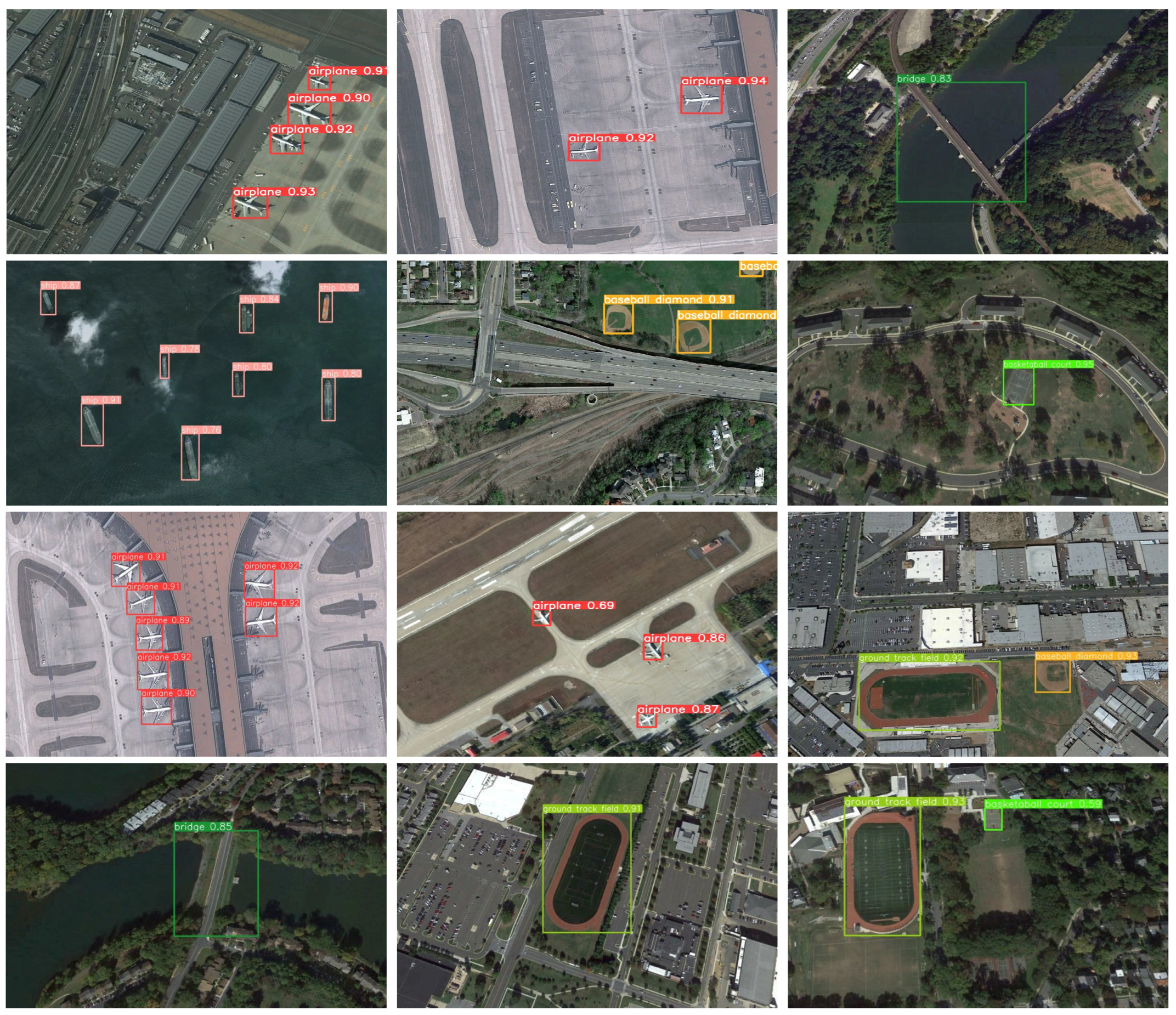
The NWPU VHR-10 dataset [49] is a remote sensing dataset introduced by the Northwestern Polytechnical University (NWPU), comprising 10 categories of remotely sensed feature objects such as airplanes, ships, baseball fields, and more. It comprises 800 ultra-high resolution images containing 3651 annotated objects. These images have been extracted and labeled from the Google Earth and Vaihingen datasets. Figure 10 shows some images of the dataset and the box illustrating the detection results of RS-FeatFuseNet algorithm. Notably, both large-scale and small-scale objects exhibit notably accurate detection results within the depicted images.
Our study involved thorough experiments with the YOLOv8n and RS-FeatFuseNet on the dataset. Table 5 shows the detection results of RS-FeatFuseNet on each specific category in the dataset.
We provide a detailed analysis of how the RS-FeatFuseNet algorithm performed to enable a comprehensive evaluation. Significant findings from Table 6 include a 7% increase in the mAP@50 for harbor category and a 5.9% boost for the bridge category after implementing RS-FeatFuseNet. Additionally, an overall improvement of 0.8% in the mAP@50 score across all categories highlights the effectiveness of RS-FeatFuseNet.

4.1.3. VEDAI

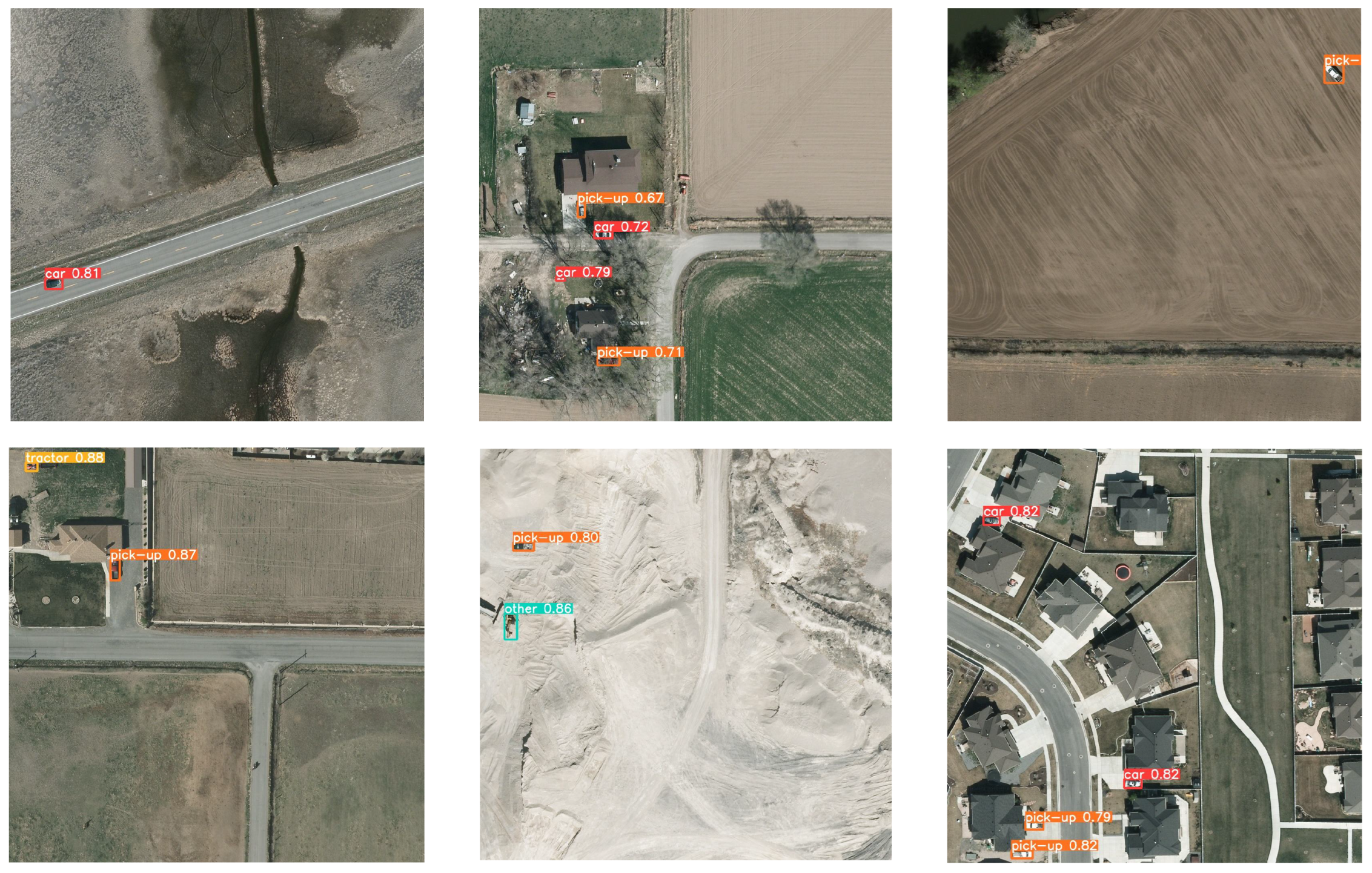
The VEDAI [50] dataset was proposed for the task of detecting small vehicles in aerial images. Figure 11 shows some images of the dataset. It includes various complex backgrounds such as forests, construction sites, and fields. The detected vehicles exhibit different orientations and may also encounter occlusions, changes in lighting conditions, and other challenges. This dataset comprises nine categories with a total of 3640 instances. Each image contains four uncompressed color channels and is provided in two sizes: 1024 × 1024 and 512 × 512. In this study, we utilized images of size 1024 × 1024.
Figure 11 and Table 7 showcase the performance of RS-FeatFuseNet on the VEDAI dataset. The experimental findings indicate that the mAP@50 value for ‘car’ stands out as the highest at 90.7%, while the ‘other’ class exhibits the lowest mAP@50 value at 43%. This disparity is likely attributed to the scarcity of samples in the ‘other’ class, as the remaining categories demonstrate promising results.
Table 8 presents the experimental results of our RS-FeatFuseNet algorithm compared to the YOLOv8 algorithm on the VEDAI dataset. The results indicate that the enhanced algorithm shows a decrease in performance for ‘pick-up’ and ‘car’, while there are improvements in the mAP@50 values for other categories. Particularly noteworthy is the significant increase of 11.4% in the ‘tractor’ category. Overall, the mAP@50 value has increased by 2.8%.

4.2. Experimental Validation of the ESHA and PFEM

We verified the role of the ESHA module in improving the performance of models under different basic model architectures by comparing the performance differences of various models with and without the ESHA module. The experimental results in the Table 9 demonstrate the performance comparison on the DIOR dataset before and after integrating the ESHA module across different backbone models. It is evident from the table that almost all models show improvements in precision, recall, mAP@50, and mAP@50-95 metrics when integrated into the YOLOv5, YOLOv3, YOLOv8, GhostNet, and MobileNetv3 models. YOLOv8 achieves an mAP@50 of 88.7%. Integrating ESHA into YOLOv5 leads to an 8.3% increase in precision, a 1.3% increase in recall, and a 4.9% increase in mAP@50. Furthermore, there is an 8.7% improvement in mAP@50-95, demonstrating the effectiveness of our module. With the addition of the ESHA module to YOLOv3, there is a 3% increase in mAP@50. This indicates that our ESHA module exhibits strong generalization capabilities.
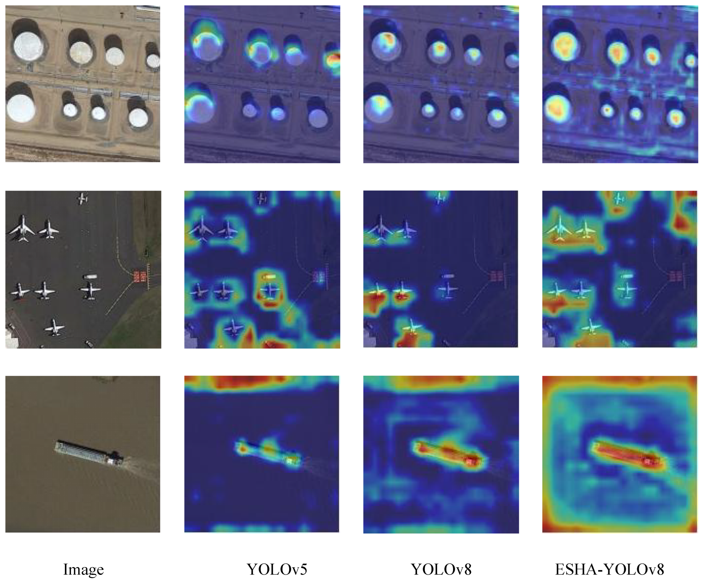
To demonstrate the efficacy of the ESHA module for feature extraction, we visualized its impact on three models—YOLOv5, YOLOv8, and YOLOv8-ESHA using select images from the DIOR dataset. As we can see from Figure 12, we generated heat maps with GradCAM at the last layer of feature extraction for the three models and overlaid them on the original images. The lighter regions within the heat maps signify areas where the model focuses more intently, while darker regions indicate areas of lesser focus. Upon comparing the heat maps, it becomes apparent that after integrating the ESHA module, the model allocates energy more prominently within the object regions with additional attention dispersed across the surrounding background. This observation suggests that the enhanced network excels in extracting global features compared to its pre-improved counterpart. The ESHA module notably enhances the model’s performance to a noticeable extent.
To verify the role of the PFEM module proposed by us in improving the performance of models under different basic model architectures, we incorporated the C2f structure improved by PFEM. We conducted ablation experiments on the DIOR dataset, integrating improved C2f into the YOLOv5, YOLOv3, YOLOv8, GhostNet, and MobileNetv3 models in the neck section. The experimental results are presented in Table 10. It is evident that upon integrating the PFEM module into various backbone networks, all models demonstrate significant improvements in the below four metrics.

4.3. Experiment on Loss_Function

To select the appropriate gamma value in Equation (6), we conducted an ablation experiment. The experimental results are shown in the Table 11. Experiments were performed with gamma values of 0.3, 0.4, 0.5, 0.6 and 0.7, respectively. From the experimental results, it is evident that when gamma is set to 0.5, both mAP@50 and mAP@50-95 achieved their highest values, at 89.1 and 65.4, respectively. Therefore, we chose gamma as 0.5.
To examine the superiority of the F o c a l _ C I o U approach we employed, we not only evaluated the network performance before and after the integration of C I o U , but also conducted comparative experiments using various loss functions. The results indicate that F o c a l _ C I o U stands out as the most effective loss function. The experimental results are shown in Table 12. We believe it excels in addressing the issue of sample imbalance. When the YOLOv8 model was equipped with the C I o U , subsequent additions of the SIoU [51], GIoU [52], and WIoU loss functions [53] did not lead to an improvement in the model’s mAP@50, and in some cases, a slight decrease was observed. However, upon incorporating the F o c a l _ C I o U loss function, there was a slight enhancement, validating the effectiveness of the F o c a l _ C I o U function. In our research, it is speculated that the traditional SIoU, GIoU, and WIoU loss functions may not effectively enhance the accuracy of remote sensing object detection in complex backgrounds compared to F o c a l _ C I o U due to their primary focus on matching between bounding boxes without fully addressing class imbalance and the handling of difficult samples in complex backgrounds. Particularly in remote sensing scenarios where backgrounds are intricate and diverse, difficult samples may be relatively numerous and difficult to detect, and the limitations of traditional loss functions in capturing this complexity might restrict detection performance. On the other hand, F o c a l _ C I o U combines the class-balancing mechanism of focal loss with the target localization capability of C I o U . By diminishing the weight of samples that are easily classified and improving the handling of bounding box matching and localization, F o c a l _ C I o U enhances the accuracy of remote sensing object detection. This comprehensive consideration of class imbalance and target localization in the loss function design likely contributes to the superior performance of F o c a l _ C I o U in complex remote sensing object detection tasks.

4.4. Ablation Experiments

To explore the effectiveness of enhancement modules, we carried out ablation experiments and individual enhancement experiments on the added modules. The experimental findings suggest that strategies such as integrating the ESHA module, improving C2f, and utilizing focal loss can be beneficial. Table 13 illustrates the variations in experimental accuracy following the incorporation of different modules. After the incorporation of ESHA, the model exhibited a 0.7% improvement in mAP@50 and a 1.0 increase in recall. Despite this, there was only a slight 0.2 enhancement in GFPLOS, showcasing its strong balance between speed and accuracy. Furthermore, with the addition of the PFEM module alone, the model’s mAP@50 also rose by 0.4% with a mere 0.5 increase in GFLOPS. Moreover, by incorporating the PFEM module and employing the focal_loss function, the model’s mAP@50 improved by 1.1%, showcasing optimal performance in the experiments. The experimental data also indicate only a slight increase in GFLOPS, indicating the superiority of our model for future deployment on hardware platforms.

4.5. Comparative Experiments

4.5.1. Comparative Experiments on DIOR Dataset

We have chosen the classic single-stage algorithm SSD and the well-known two-stage algorithm Fast R-CNN for comparison. Given that our algorithm is built upon YOLOv8, we opted for the more advanced YOLOv9 and YOLOv10 in contrast to the baseline. Moreover, we incorporated the classic RT-DETR algorithm from the Transformer domain, the YOLO series algorithms that have been enhanced with Transformer, as well as the latest MFANet algorithm in the field of remote sensing. This comprehensive selection enables us to thoroughly assess the performance of our algorithm against a range of currently popular algorithms. From Table 14 and Figure 13, our algorithm shows superior performance in terms of mAP@50, achieving 89.1%, surpassing even the YOLOv10n algorithm. Regarding computational resource utilization, our algorithm exhibits a modest 1.6 increase in GFLOPS compared to the YOLOv5n algorithm with a noteworthy improvement of 6.6% in mAP@50. The experiment denotes that RS-FeatFuseNet not only improves on the original YOLOv8 algorithm model but also surpasses the latest YOLOv9 and YOLOv10 algorithms in accuracy, recall, and mAP@50. Compared to other Transformer-based algorithms such as YOLOv5s-Transformer and NPMMR-Det, our mAP@50 outperforms. While the Transformer-based RT-DETR achieves a slightly higher mAP@50 than RS-FeatFuseNet by 0.4%, the computational resources it requires far exceed those of RS-FeatFuseNet. Our algorithm strikes the best balance between speed and accuracy.

4.5.2. Comparative Experiments on NWPU VHR-10 Dataset

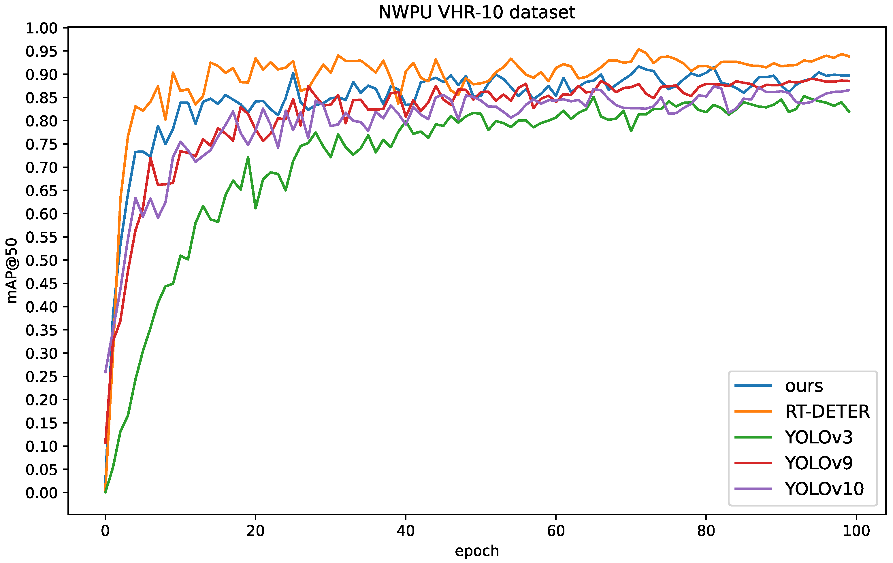
Table 15 and Figure 14 show a comparative experiment between RS-FeatFuseNet and other models. From Table 13, it can be observed that Transformer-based model RT-DETR achieved the highest score, surpassing RS-FeatFuseNet by 0.5%. However, its GFLOPS value is significantly higher. Two other Transformer-based models, YOLOv5s-Transformer and NPMMR-Det, have lower accuracy than our model. Comparing to the two-stage algorithm Fast R-CNN, our algorithm exhibits notable advantages, showcasing lower GFLOPS consumption along with higher mAP@50 and mAP@50-95 scores. From a practical application perspective, our algorithm has an advantage in inference speed.

4.5.3. Comparative Experiments on VEDAI Dataset

Table 16 presents the experimental results of our RS-FeatFuseNet compared to other algorithms. The results demonstrate that FFCA-YOLO achieves the highest mAP@50, reaching 75.6%. However, in comparison to our model, FFCA-YOLO has over three times higher GFLOPS, while our model only lags by 2.4% in mAP@50. Furthermore, other Transformer-based models such as RT-DETR and TPH-YOLO fall short in both accuracy and resource consumption when compared to our model. Overall, our RS-FeatFuseNet delivers the best performance.
Figure 15 depicts examples of detection results on the DIOR dataset for RT-DETR, YOLOv10, Fast R-CNN and RS-FeatFuseNet. In the first set of images, YOLOv10 missed detecting the “harbor”. In the second set of images, both RT-DETR and YOLOv10 failed to detect targets such as “vehicles” and “harbor”. However, in the final set of images, only RT-DETR and our RS-FeatFuseNet successfully detected the “trainstation”. Moreover, considering the overall detection confidence, our proposed RS-FeatFuseNet achieved the highest.

5. Discussion

5.1. Small Objects Detection

Although some improvements have been made in feature enhancement and certain enhancements have been achieved, in-depth experiments on dedicated remote sensing small object datasets have not been carried out yet. And as can be seen from the experimental results, within the DIOR dataset, although our improvements have led to an increase in mAP@50, the detection results of “vehicle” with relatively small target sizes are not as ideal as those of other categories. We speculate that in addition to the reason of feature insufficiency that our paper mainly focuses on, it is also possible that small targets are prone to losing information during the upsampling process, which will have a significant impact on small targets that already have relatively little information. Therefore, in the next stage of our work, we plan to conduct further experimental improvements specifically targeting small objects. Currently, there are some papers that use wavelet transform to replace upsampling to achieve lossless upsampling. Hence, our next goal is to see whether it can be applied to remote sensing target detection. Meanwhile, we also plan to continue our research from the aspect of the attention mechanism to make the network pay more attention to valuable information.

5.2. The Optimization Strategy of Remote Sensing Loss Function Based on Object Scale

In terms of the loss function, we have only made improvements regarding the imbalance between difficult and easy samples for now without taking into account the issue of the diversity of remote sensing target scales. Therefore, we hope to design a mechanism that can dynamically adjust the parameters of the loss function according to the target scale. For example, for targets with relatively large scales, the penalty term in F o c a l _ C I o U can focus on the position accuracy of the bounding box. While for small-scale targets, in addition to the position accuracy, the penalty for the discrimination degree between the target and the background can be strengthened. In this way, the loss function can better adapt to the characteristics of targets with different scales.

6. Conclusions

Considering that the shooting scenes of remote sensing images are complex and changeable, this paper designs a module named effective multi-scales and multi-head attention (ESHA) that can be used to help identify targets in complex backgrounds. Based on multi-scale attention, this module introduces multi-head self-attention (MHSA) to extract global features. It can not only better capture the relationship between objects and backgrounds but also extract and help with global semantic information, assist the model in understanding the positions and features of objects in complex backgrounds, enhance the model’s perception ability of complex scenes, and better adapt to remote sensing images of different scales and complexity levels. Meanwhile, considering the characteristics of remote sensing images, such as having numerous small targets and fewer features, this paper optimizes the C2f module in the neck section of the YOLOv8 network by adding the Parallel Feature Enhancement Module (PFEM). This broadens the receptive field without increasing the network depth and enhances network features. In addition, we improve the loss function and increase the weights of samples that are difficult to classify, thereby improving the detection accuracy of the network. Experiments show that the performance of our improved network, RS-FeatFuseNet, has been significantly improved on three remote sensing datasets. Compared with some other popular detection algorithms, it also has a relatively significant advantage.

Author Contributions

Conceptualization, Y.Q.; Data curation, Y.Q. and J.X.; Investigation, Y.Q., T.L. and P.J.; Methodology, Y.Q.; Software, Y.Q.; Writing—original draft, Y.Q.; Writing—review and editing, G.Z. and X.H. All authors have read and agreed to the published version of the manuscript.

Funding

This research received no external funding.

Data Availability Statement

The original contributions presented in the study are included in the article, further inquiries can be directed to the corresponding author.

Conflicts of Interest

The authors declare no conflicts of interest.

References

  1. Zhang, B.; Wu, Y.; Zhao, B.; Chanussot, J.; Hong, D.; Yao, J.; Gao, L. Progress and challenges in intelligent remote sensing satellite systems. IEEE J. Sel. Top. Appl. Earth Obs. Remote Sens. 2022, 15, 1814–1822. [Google Scholar] [CrossRef]
  2. Wang, B.; Zhao, Y.; Li, X. Multiple instance graph learning for weakly supervised remote sensing object detection. IEEE Trans. Geosci. Remote Sens. 2021, 60, 1–12. [Google Scholar] [CrossRef]
  3. Niu, R.; Zhi, X.; Jiang, S.; Gong, J.; Zhang, W.; Yu, L. Aircraft target detection in low signal-to-noise ratio visible remote sensing images. Remote Sens. 2023, 15, 1971. [Google Scholar] [CrossRef]
  4. Huang, W.; Huang, Y.; Wang, H.; Liu, Y.; Shim, H.J. Local binary patterns and superpixel-based multiple kernels for hyperspectral image classification. IEEE J. Sel. Top. Appl. Earth Obs. Remote Sens. 2020, 13, 4550–4563. [Google Scholar] [CrossRef]
  5. Cheng, G.; Han, J. A survey on object detection in optical remote sensing images. ISPRS J. Photogramm. Remote Sens. 2016, 117, 11–28. [Google Scholar] [CrossRef]
  6. Li, C.; Cong, R.; Guo, C.; Li, H.; Zhang, C.; Zheng, F.; Zhao, Y. A parallel down-up fusion network for salient object detection in optical remote sensing images. Neurocomputing 2020, 415, 411–420. [Google Scholar] [CrossRef]
  7. Goyal, A.; Bochkovskiy, A.; Deng, J.; Koltun, V. Non-deep networks. Adv. Neural Inf. Process. Syst. 2022, 35, 6789–6801. [Google Scholar]
  8. Ouyang, D.; He, S.; Zhang, G.; Luo, M.; Guo, H.; Zhan, J.; Huang, Z. Efficient multi-scale attention module with cross-spatial learning. In Proceedings of the ICASSP 2023-2023 IEEE International Conference on Acoustics, Speech and Signal Processing (ICASSP), Rhodes Island, Greece, 4–10 June 2023; pp. 1–5. [Google Scholar]
  9. Zhu, X.; Lyu, S.; Wang, X.; Zhao, Q. TPH-YOLOv5: Improved YOLOv5 based on transformer prediction head for object detection on drone-captured scenarios. In Proceedings of the IEEE/CVF International Conference on Computer Vision, Montreal, BC, Canada, 11–17 October 2021; pp. 2778–2788. [Google Scholar]
  10. Girshick, R.; Donahue, J.; Darrell, T.; Malik, J. Region-based convolutional networks for accurate object detection and segmentation. IEEE Trans. Pattern Anal. Mach. Intell. 2015, 38, 142–158. [Google Scholar] [CrossRef] [PubMed]
  11. Girshick, R. Fast r-cnn. In Proceedings of the IEEE International Conference on Computer Vision, Santiago, Chile, 7–13 December 2015; pp. 1440–1448. [Google Scholar]
  12. Ren, S.; He, K.; Girshick, R.; Sun, J. Faster r-cnn: Towards real-time object detection with region proposal networks. Adv. Neural Inf. Process. Syst. 2015, 28, 1–9. [Google Scholar] [CrossRef] [PubMed]
  13. He, K.; Gkioxari, G.; Dollár, P.; Girshick, R. Mask r-cnn. In Proceedings of the IEEE International Conference on Computer Vision, Venice, Italy, 22–29 October 2017; pp. 2961–2969. [Google Scholar]
  14. Vaswani, A.; Shazeer, N.; Parmar, N.; Uszkoreit, J.; Jones, L.; Gomez, A.N.; Kaiser, Ł.; Polosukhin, I. Attention is all you need. Adv. Neural Inf. Process. Syst. 2017, 30, 1–11. [Google Scholar]
  15. Dosovitskiy, A.; Beyer, L.; Kolesnikov, A.; Weissenborn, D.; Zhai, X.; Unterthiner, T.; Dehghani, M.; Minderer, M.; Heigold, G.; Gelly, S.; et al. An image is worth 16x16 words: Transformers for image recognition at scale. arXiv 2020, arXiv:2010.11929. [Google Scholar]
  16. Lin, T.Y.; Dollár, P.; Girshick, R.; He, K.; Hariharan, B.; Belongie, S. Feature pyramid networks for object detection. In Proceedings of the IEEE Conference on Computer Vision and Pattern Recognition, Honolulu, HI, USA, 21–26 July 2017; pp. 2117–2125. [Google Scholar]
  17. Weng, L.; Gao, J.; Xia, M.; Lin, H. MSNet: Multifunctional Feature-Sharing Network for Land-Cover Segmentation. Remote Sens. 2022, 14, 5209. [Google Scholar] [CrossRef]
  18. Yan, D.; Li, G.; Li, X.; Zhang, H.; Lei, H.; Lu, K.; Cheng, M.; Zhu, F. An improved faster R-CNN method to detect tailings ponds from high-resolution remote sensing images. Remote Sens. 2021, 13, 2052. [Google Scholar] [CrossRef]
  19. Yin, S.; Li, H.; Teng, L. Airport detection based on improved faster RCNN in large scale remote sensing images. Sens. Imaging 2020, 21, 49. [Google Scholar] [CrossRef]
  20. Wang, Y.; Peng, J.; Wang, H.; Wang, M. Progressive learning with multi-scale attention network for cross-domain vehicle re-identification. Sci. China Inf. Sci. 2022, 65, 160103. [Google Scholar] [CrossRef]
  21. Peng, J.; Wang, Y.; Wang, H.; Zhang, Z.; Fu, X.; Wang, M. Unsupervised vehicle re-identification with progressive adaptation. arXiv 2020, arXiv:2006.11486. [Google Scholar]
  22. Ren, Y.; Zhu, C.; Xiao, S. Small object detection in optical remote sensing images via modified faster R-CNN. Appl. Sci. 2018, 8, 813. [Google Scholar] [CrossRef]
  23. Tan, M.; Pang, R.; Le, Q.V. Efficientdet: Scalable and efficient object detection. In Proceedings of the IEEE/CVF Conference on Computer Vision and Pattern Recognition, Seattle, WA, USA, 13–19 June 2020; pp. 10781–10790. [Google Scholar]
  24. Radosavovic, I.; Kosaraju, R.P.; Girshick, R.; He, K.; Dollár, P. Designing network design spaces. In Proceedings of the IEEE/CVF Conference on Computer Vision and Pattern Recognition, Seattle, WA, USA, 13–19 June 2020; pp. 10428–10436. [Google Scholar]
  25. Rabbi, J.; Ray, N.; Schubert, M.; Chowdhury, S.; Chao, D. Small-object detection in remote sensing images with end-to-end edge-enhanced GAN and object detector network. Remote Sens. 2020, 12, 1432. [Google Scholar] [CrossRef]
  26. Liu, J.; Li, S.; Zhou, C.; Cao, X.; Gao, Y.; Wang, B. SRAF-Net: A scene-relevant anchor-free object detection network in remote sensing images. IEEE Trans. Geosci. Remote Sens. 2021, 60, 1–14. [Google Scholar] [CrossRef]
  27. Redmon, J.; Divvala, S.; Girshick, R.; Farhadi, A. You only look once: Unified, real-time object detection. In Proceedings of the IEEE Conference on Computer Vision and Pattern Recognition, Las Vegas, NV, USA, 27–30 June 2016; pp. 779–788. [Google Scholar]
  28. Redmon, J.; Farhadi, A. Yolov3: An incremental improvement. arXiv 2018, arXiv:1804.02767. [Google Scholar]
  29. Bochkovskiy, A.; Wang, C.Y.; Liao, H.Y.M. Yolov4: Optimal speed and accuracy of object detection. arXiv 2020, arXiv:2004.10934. [Google Scholar]
  30. Zhang, Y.; Guo, Z.; Wu, J.; Tian, Y.; Tang, H.; Guo, X. Real-time vehicle detection based on improved yolo v5. Sustainability 2022, 14, 12274. [Google Scholar] [CrossRef]
  31. Wang, C.Y.; Yeh, I.H.; Liao, H.Y.M. Yolov9: Learning what you want to learn using programmable gradient information. arXiv 2024, arXiv:2402.13616. [Google Scholar]
  32. Wang, A.; Chen, H.; Liu, L.; Chen, K.; Lin, Z.; Han, J.; Ding, G. Yolov10: Real-time end-to-end object detection. arXiv 2024, arXiv:2405.14458. [Google Scholar]
  33. Liu, W.; Anguelov, D.; Erhan, D.; Szegedy, C.; Reed, S.; Fu, C.Y.; Berg, A.C. Ssd: Single shot multibox detector. In Proceedings of the Computer Vision–ECCV 2016: 14th European Conference, Amsterdam, The Netherlands, 11–14 October 2016; Proceedings, Part I 14. Springer: Berlin/Heidelberg, Germany, 2016; pp. 21–37. [Google Scholar]
  34. Lin, T.Y.; Goyal, P.; Girshick, R.; He, K.; Dollár, P. Focal loss for dense object detection. In Proceedings of the IEEE International Conference on Computer Vision, Venice, Italy, 22–29 October 2017; pp. 2980–2988. [Google Scholar]
  35. Lang, K.; Cui, J.; Yang, M.; Wang, H.; Wang, Z.; Shen, H. A Convolution with Transformer Attention Module Integrating Local and Global Features for Object Detection in Remote Sensing Based on YOLOv8n. Remote Sens. 2024, 16, 906. [Google Scholar] [CrossRef]
  36. Huo, B.; Li, C.; Zhang, J.; Xue, Y.; Lin, Z. SAFF-SSD: Self-attention combined feature fusion-based SSD for small object detection in remote sensing. Remote Sens. 2023, 15, 3027. [Google Scholar] [CrossRef]
  37. Woo, S.; Park, J.; Lee, J.Y.; Kweon, I.S. Cbam: Convolutional block attention module. In Proceedings of the European Conference on Computer Vision (ECCV), Munich, Germany, 8–14 September 2018; pp. 3–19. [Google Scholar]
  38. Zhang, Y.; Ye, M.; Zhu, G.; Liu, Y.; Guo, P.; Yan, J. FFCA-YOLO for small object detection in remote sensing images. IEEE Trans. Geosci. Remote Sens. 2024, 62, 5611215. [Google Scholar] [CrossRef]
  39. Shen, L.; Lang, B.; Song, Z. CA-YOLO: Model optimization for remote sensing image object detection. IEEE Access 2023, 11, 64769–64781. [Google Scholar] [CrossRef]
  40. Lai, H.; Chen, L.; Liu, W.; Yan, Z.; Ye, S. STC-YOLO: Small object detection network for traffic signs in complex environments. Sensors 2023, 23, 5307. [Google Scholar] [CrossRef] [PubMed]
  41. Ross, T.Y.; Dollár, G. Focal loss for dense object detection. In Proceedings of the IEEE Conference on Computer Vision and Pattern Recognition, Honolulu, HI, USA, 21–26 July 2017; pp. 2980–2988. [Google Scholar]
  42. Law, H.; Deng, J. Cornernet: Detecting objects as paired keypoints. In Proceedings of the European Conference on Computer Vision (ECCV), Munich, Germany, 8–14 September 2018; pp. 734–750. [Google Scholar]
  43. Wang, P.; Sun, X.; Diao, W.; Fu, K. FMSSD: Feature-merged single-shot detection for multiscale objects in large-scale remote sensing imagery. IEEE Trans. Geosci. Remote Sens. 2019, 58, 3377–3390. [Google Scholar] [CrossRef]
  44. Liu, Z.; Lin, Y.; Cao, Y.; Hu, H.; Wei, Y.; Zhang, Z.; Lin, S.; Guo, B. Swin transformer: Hierarchical vision transformer using shifted windows. In Proceedings of the IEEE/CVF International Conference on Computer Vision, Montreal, BC, Canada, 11–17 October 2021; pp. 10012–10022. [Google Scholar]
  45. Dong, X.; Bao, J.; Chen, D.; Zhang, W.; Yu, N.; Yuan, L.; Chen, D.; Guo, B. Cswin transformer: A general vision transformer backbone with cross-shaped windows. In Proceedings of the IEEE/CVF Conference on Computer Vision and Pattern Recognition, New Orleans, LA, USA, 18–24 June 2022; pp. 12124–12134. [Google Scholar]
  46. Wang, G.; Chen, H.; Chen, L.; Zhuang, Y.; Zhang, S.; Zhang, T.; Dong, H.; Gao, P. P 2fevit: Plug-and-play cnn feature embedded hybrid vision transformer for remote sensing image classification. Remote Sens. 2023, 15, 1773. [Google Scholar] [CrossRef]
  47. Xu, X.; Feng, Z.; Cao, C.; Li, M.; Wu, J.; Wu, Z.; Shang, Y.; Ye, S. An improved swin transformer-based model for remote sensing object detection and instance segmentation. Remote Sens. 2021, 13, 4779. [Google Scholar] [CrossRef]
  48. Li, K.; Wan, G.; Cheng, G.; Meng, L.; Han, J. Object detection in optical remote sensing images: A survey and a new benchmark. ISPRS J. Photogramm. Remote Sens. 2020, 159, 296–307. [Google Scholar] [CrossRef]
  49. Cheng, G.; Han, J.; Zhou, P.; Guo, L. Multi-class geospatial object detection and geographic image classification based on collection of part detectors. ISPRS J. Photogramm. Remote Sens. 2014, 98, 119–132. [Google Scholar] [CrossRef]
  50. Razakarivony, S.; Jurie, F. Vehicle detection in aerial imagery: A small target detection benchmark. J. Vis. Commun. Image Represent. 2016, 34, 187–203. [Google Scholar] [CrossRef]
  51. Gevorgyan, Z. SIoU loss: More powerful learning for bounding box regression. arXiv 2022, arXiv:2205.12740. [Google Scholar]
  52. Rezatofighi, H.; Tsoi, N.; Gwak, J.; Sadeghian, A.; Reid, I.; Savarese, S. Generalized intersection over union: A metric and a loss for bounding box regression. In Proceedings of the IEEE/CVF Conference on Computer Vision and Pattern Recognition, Long Beach, CA, USA, 15–20 June 2019; pp. 658–666. [Google Scholar]
  53. Tong, Z.; Chen, Y.; Xu, Z.; Yu, R. Wise-IoU: Bounding box regression loss with dynamic focusing mechanism. arXiv 2023, arXiv:2301.10051. [Google Scholar]
  54. Fan, C.; Fang, Z. Probability-Enhanced Anchor-Free Detector for Remote-Sensing Object Detection. Comput. Mater. Contin. 2024, 79, 4925–4943. [Google Scholar] [CrossRef]
  55. Wang, C.; He, W.; Nie, Y.; Guo, J.; Liu, C.; Wang, Y.; Han, K. Gold-YOLO: Efficient object detector via gather-and-distribute mechanism. Adv. Neural Inf. Process. Syst. 2024, 36, 1–19. [Google Scholar]
  56. Chen, Y.; Yuan, X.; Wu, R.; Wang, J.; Hou, Q.; Cheng, M.M. Yolo-ms: Rethinking multi-scale representation learning for real-time object detection. arXiv 2023, arXiv:2308.05480. [Google Scholar]
  57. Wang, K.; Bai, F.; Li, J.; Liu, Y.; Li, Y. MashFormer: A novel multiscale aware hybrid detector for remote sensing object detection. IEEE J. Sel. Top. Appl. Earth Obs. Remote Sens. 2023, 16, 2753–2763. [Google Scholar] [CrossRef]
  58. Lyu, C.; Zhang, W.; Huang, H.; Zhou, Y.; Wang, Y.; Liu, Y.; Zhang, S.; Chen, K. Rtmdet: An empirical study of designing real-time object detectors. arXiv 2022, arXiv:2212.07784. [Google Scholar]
Figure 1. Some Instances of remote sensing objects. (a) Complex backgrounds; (b) sparse information in small objects; (c) varied scales.
Remotesensing 17 00061 g001
Figure 2. Structure of the RS-FeatFuseNet.
Remotesensing 17 00061 g002
Figure 3. The Architecture of ESHA. (a) ESHA is our designed attention module. (b) The architecture of EMA. The feature map first undergoes processing by the EMA module to extract multi-scale attention; (c) the architecture of MHSA. The processed attention is then input into the MHSA module for long-range attention extraction before being output. x represents the multiplication operation.
Remotesensing 17 00061 g003
Figure 4. The structure of C2f.
Remotesensing 17 00061 g004
Figure 5. The structure of improved bottleneck and PFEM. (a) Comparison of bottleneck before and after improvement; (b) the structure of PFEM; X represents multiplication operation, while A represents addition operation.
Remotesensing 17 00061 g005
Figure 6. IoU is represented by a graphic.
Remotesensing 17 00061 g006
Figure 7. C I o U is represented by a graphic. where ‘d’ denotes the Euclidean distance between the geometric centroids of the ground truth box and the predicted bounding box. Meanwhile, ‘C’ represents the length of the diagonal within the minimal enclosing rectangles that circumscribe both the aforesaid boxes.
Remotesensing 17 00061 g007
Figure 8. Object size distribution of DIOR [48].
Remotesensing 17 00061 g008
Figure 9. Detection results of RS-FeatFuseNet on the DIOR dataset [48].
Remotesensing 17 00061 g009
Figure 10. Detection results of RS-FeatFuseNet on the NWPU VHR-10 [49] dataset.
Remotesensing 17 00061 g010
Figure 11. Detection results of RS-FeatFuseNet on the VEDAI dataset [50].
Remotesensing 17 00061 g011
Figure 12. Heat map visualization of the partial detection results before and after adding the ESHA module.
Remotesensing 17 00061 g012
Figure 13. Comparison experiments on DIOR.
Remotesensing 17 00061 g013
Figure 14. Comparison experiments on NWPU VHR-10 dataset.
Remotesensing 17 00061 g014
Figure 15. Comparison of detection results of RT-DETR, YOLOv10, Fast R-CNN and RS-FeatFuseNet on DIOR dataset.
Remotesensing 17 00061 g015
Table 1. Parameter setting of the RS-FeatFuseNet.
IndexModuleFromNArgvsParameters
0Conv−11[3, 16, 3, 2]464
1Conv−11[16, 32, 3, 2]4672
2C2f−11[32, 32, 1, True]7360
3Conv−11[32, 64, 3, 2]18,560
4C2f−12[64, 64, 2, True]49,664
5Conv−11[64, 128, 3, 2]73,984
6C2f−12[128, 128, 2, True]197,632
7Conv−11[128, 256, 3, 2]295,424
8C2f−11[256, 256, 1, True]460,288
9SPPF−11[256, 256, 5]164,608
10Upsample−11[None, 2, ‘nearest’]0
11Concat[−1, 6]1[1]0
12C2f−11[384, 128, 1]148,224
13Upsample−11[None, 2, ‘nearest’]0
14Concat[−1, 4]1[1]0
15Improved_C2f−11[192, 64, 1]48,736
16Conv−11[64, 64, 3, 2]36,992
17Concat[−1, 12]1[1]0
19Conv−11[128, 128, 3, 2]147,712
20Concat[−1, 9]1[1]0
21Improved_C2f−11[384, 256, 1]674,176
22ESHA−11[256, 4]198,720
23Detect[15, 18, 22]1[20, [64, 128, 256]]755,212
Table 2. Experimental platform and Configuration of the experimental environment.
PlatformName
GPUTITAN X (NVIDIA, Santa Clara, CA, USA)
CPUIntel(R) Core(TM) i7-7700K CPU
(Intel, Santa Clara, CA, USA)
The Operating Systemubuntu 18.04
Programming Languagepython 3.8
Deep Learning Frameworkpytorch 2.0
CUDA11.3
Table 3. Results of the RS-FeatFuseNet algorithm on the DIOR dataset.
CategoryPrecisionRecallmAP@50mAP@50-95
all89.28389.165.4
airplane98.591.696.273.6
airport81.485.989.463.8
baseballfield94.694.695.582
basketballfield96.192.895.987
bridge84.851.565.640.9
chimney93.591.994.686.1
Dam81.281.987.553.9
Expressway-service-area89.594.795.571.7
Expressway-toll-station91.583.189.870.1
golffield88.38894.168.7
habor80.767.378.652.4
overpass89.766.978.754.7
ship95.392.996.762.6
stadium88.39494.876.5
storagetank89.78791.262.6
tenniscourt96.791.496.384.3
trainstation74.673.97943.7
vehicle90.154.173.243.1
windmill95.787.894.452.4
Table 4. Comparison of mAP@50 of YOLOv8 algorithm before and after improvement on DIOR dataset.
MethodAllAirplaneAirportGolffield
YOLOv88896.383.489
RS-FeatFuseNet89.196.289.494.1
shipchimneygolffieldExpressway-service-areahabor
96.594.18993.377.6
96.794.694.195.578.6
Table 5. Results of the RS-FeatFuseNet algorithm on the NWPU VHR-10 dataset.
CategoryPrecisionRecallmAP@50mAP@50-95
All89.988.291.660.7
Airplane98.9199.578.2
Ship92.886.291.855.3
Storage tank99.1199.560.2
Baseball diamond91.794.397.274
Tennis court98.777.492.663.3
Basketball court81.570.478.152.6
Ground track field90.793.898.676.3
Habor77.6197.844.9
Bridge71.16463.928.1
Vehicle97.196.297.474.6
Table 6. Comparison of mAP@50 of YOLOv8 algorithm before and after improvement on NWPU VHR-10 dataset.
MethodAllAirplaneShipStorage TankHaborBridge
yolov890.899.59099.584.858
RS-FeatFuseNet91.699.591.899.597.863.9
Table 7. Results of the RS-FeatFuseNet algorithm on the VEDAI dataset.
CategoryPrecisionRecallmAP@50mAP@50-95
all72.56873.246.7
car88.282.990.760.9
truck54.561.462.241.3
pick-up71.982.982.255.2
tractor835872.338.2
camping_car73.876.178.753
boat70.170.471.946.4
van61.282.178.955.7
other49.438.34325.5
large160.378.844.1
Table 8. Comparison of results of YOLOv8 algorithm before and after improvement on VEDAI dataset.
MethodAllCarTruckPick-UpTractorCamping_CarBoatVanOtherLarge
yolov870.491.261.685.360.978.670.675.939.975.6
ours73.290.762.282.272.378.771.978.94378.8
Table 9. Experimental results on DIOR dataset of ESHA.
DatasetModelPrecisionRecallmAP@50mAP@50-95GFLOPS
DIORYOLOv578.479.782.553.57.1
YOLOv5-ESHA86.78187.462.27.8
YOLOv377.674.576.25018.9
YOLOv3-ESHA77.975.479.65319.1
YOLOv888.582.288.064.08.1
YOLOv8-ESHA88.483.288.764.68.3
GhostNet87.076.983.859.75.2
GhostNet-ESHA87.181.186.663.410.6
MoblieNetv384.073.479.954.95.7
MoblieNetv3-ESHA84.172.980.154.75.9
Table 10. Experimental results on DIOR dataset of PFEM.
DatasetModelPrecisionRecallmAP@50mAP@50-95GFLOPS
DIORYOLOv578.479.782.553.57.1
YOLOv5-PFEM84.68185.455.78.1
YOLOv377.674.576.25018.9
YOLOv3-PFEM77.875.476.954.119.6
YOLOv888.582.288648.1
YOLOv8-PFEM88.982.388.464.58.5
GhostNet87.076.983.859.75.2
GhostNet-PFEM87.078.785.061.76.8
MoblieNetv384.073.479.954.95.7
MoblieNetv3-PFEM86.074.081.457.16.2
Table 11. Ablation experiment on the gamma parameter.
γ mAP@50mAP@50-95
0.387.264.8
0.488.264.9
0.589.165.3
0.68964.9
0.788.765.1
Table 12. Experiment on different Loss_Function.
Loss_FunctionPrecisionRecallmAP@50mAP@50-95
cIoU878388.865.2
SIoU88.78388.765.2
GIoU88.183.788.865.6
WIoUv38982.688.765.4
WIoUv288.782.688.565
Focal_CIoU89.38389.165.3
Table 13. Ablation experiment on DIOR.
ModelRecallmAP@50GFLOPS
YOLOv882.2888.1
YOLOv8 + ESHA83.288.78.3
YOLOv8 + PFEM82.388.48.5
YOLOv8 + ESHA + PFEM8388.88.7
YOLOv8 + ESHA + PFEM + Focal_CIoU8389.18.7
Table 14. Comparison experiments on DIOR dataset.
ModelmAP@50GFLOPS
SSD73.459.4
Fast R-CNN80180.2
YOLOv376.218.9
YOLOv5n82.57.1
YOLOv8n888.1
YOLOv9t87.911.1
YOLOv10n88.98.3
MFANet [54]87.88
Gold-YOLO [55]83.112.3
YOLO-MS [56]80.915.7
YOLOv5s-Transformer88.552.5
RT-DETR88.7108.1
Ours89.18.7
Table 15. Comparison experiments on NWPU dataset.
ModelmAP@50GFLOPS
SSD86.759.4
Fast R-CNN88.3180.2
YOLOv385.418.9
YOLOv8n90.88.1
YOLOv9t88.410.7
YOLOv10n87.28.2
TPH-YOLO [57]88.2249.2
RMEDet [58]87.98.1
RT-DETR92103.5
Ours91.58.7
Table 16. Comparison experiments on VEDAI dataset.
ModelmAP@50GFLOPS
Fast R-CNN46.1195
Yolov354.213.1
Yolov5n51.45.9
Yolov8n70.48.3
Yolov9t65.111.2
Yolov10n72.48.3
FFCA-YOLO75.628.6
TPH-YOLO62.0249.1
RT-DETR46.5104
Ours73.28.7
Disclaimer/Publisher’s Note: The statements, opinions and data contained in all publications are solely those of the individual author(s) and contributor(s) and not of MDPI and/or the editor(s). MDPI and/or the editor(s) disclaim responsibility for any injury to people or property resulting from any ideas, methods, instructions or products referred to in the content.