Enhancing Binary Change Detection in Hyperspectral Images Using an Efficient Dimensionality Reduction Technique Within Adversarial Learning

Abstract

Detecting binary changes in co-registered bitemporal hyperspectral images (HSIs) using deep learning methods is challenging due to the high dimensionality of spectral data and significant variations between images. To address this challenge, previous approaches often used dimensionality reduction methods separately from the change detection network, leading to less accurate results. In this study, we propose an end-to-end fully connected adversarial network (EFC-AdvNet) for binary change detection, which efficiently reduces the dimensionality of bitemporal HSIs and simultaneously detects changes between them. This is accomplished by extracting critical spectral features at the pixel level through a self-spectral reconstruction (SSR) module working in conjunction with an adversarial change detection (Adv-CD) module to effectively delineate changes between bitemporal HSIs. The SSR module employs a fully connected autoencoder for hyperspectral dimensionality reduction and spectral feature extraction. By integrating the encoder segment of the SSR module with the change detection network of the Adv-CD module, we create a generator that directly produces highly accurate change maps. This joint learning approach enhances both feature extraction and change detection capabilities. The proposed network is trained using a comprehensive loss function derived from the concurrent learning of the SSR and Adv-CD modules, establishing EFC-AdvNet as a robust end-to-end network for hyperspectral binary change detection. Experimental evaluations of EFC-AdvNet on three public hyperspectral datasets demonstrate that joint learning between the SSR and Adv-CD modules improves the overall accuracy (OA) by 5.44%, 10.43%, and 7.52% for the Farmland, Hermiston, and River datasets, respectively, compared with the separate learning approach.

1. Introduction

Hyperspectral imaging is a powerful technique that allows for the collection and analysis of detailed spectral information for each pixel in an image. This technique captures images across a wide range of wavelengths in the electromagnetic spectrum, providing valuable information about the composition and characteristics of objects or materials in a scene. By measuring and analyzing the reflected radiation at different wavelengths, hyperspectral images (HSIs) enable the detection and differentiation of unique materials with high accuracy [1]. One important application of HSIs is change detection, which involves comparing multiple HSIs taken at different times to identify and analyze changes in a scene over time. This analysis can be applied to various fields, such as agriculture, environmental monitoring, urban planning, and defense. The main objective of change detection in HSIs is to detect and quantify the changes in the spectral properties of objects or materials in a scene. These changes may be indicative of land-cover changes, environmental changes, or other significant events that can provide valuable insights for decision-making processes. Various methods and algorithms have been developed for detecting changes in HSIs [2].

1.1. Traditional vs. Deep Learning Approaches in Hyperspectral Change Detection

Traditional change detection methods typically involve two main steps: generating a difference image (DI) and analyzing it to produce a binary or multiclass change map (CM) [3]. For HSIs, these operations are performed at the pixel-vector level. The process of generating a DI typically involves calculating the Euclidean distance between pixels, which is a method known as change vector analysis (CVA) [4]. While CVA effectively captures all relevant change information, it can also introduce some noise. Principal component analysis (PCA) [5] is another technique used to reduce dimensions, but it is sensitive to the statistical properties of the image and unbalanced data. Iteratively reweighed multivariate alteration detection (IR-MAD) [6] is another method that assigns different weights to observations iteratively, resulting in greater stability, but it potentially overlooks the relationship between bitemporal bands. With regard to DI binarization, clustering algorithms such as K-means, fuzzy c-means, and fuzzy local information c-means (FLICM) [7] can be effective in preserving change information while eliminating noise.

These methods rely on handcrafted features and predefined thresholds, which may not effectively capture the complex and subtle changes present in the data and cannot exploit the spectral information in HSIs, thereby limiting their ability to detect changes based on spectral signatures. Recently, deep learning (DL)-based methods have shown great promise in the field of change detection in HSIs. For instance, convolutional neural networks (CNNs) are particularly effective for learning hierarchical representations of spatial–spectral features from HSIs [8]. CNNs can automatically extract relevant features and detect changes in the spectral properties of objects or materials in a scene by applying convolutional layers and pooling operations. Several studies have explored the use of these networks and proposed various approaches, including band expansion techniques [9] and spectral–temporal transformers [10]. Additionally, there is ongoing research on developing deep learning models that can effectively detect changes by leveraging the spatial and spectral information present in HSIs, such as spectral–spatial–temporal transformers [11]. Overall, CNNs offer promising solutions for change detection in hyperspectral data with the potential for further advancements in the field [12]. Moreover, autoencoders (AEs) have also shown powerful feature extraction abilities, making it possible to establish a nonlinear complex mapping relationship [13].

1.2. Generative Adversarial Networks in Remote Sensing: Advancements and Applications in Hyperspectral Change Detection

Generative adversarial networks (GANs) [14] have recently gained widespread attention in the remote sensing domain due to their powerful generalization capabilities and their ability to learn useful representation features [15,16]. The application of adversarial networks (Adv-Nets) in change detection tasks for remote sensing data is distinguished from other methods by several key factors. For instance, adversarial training excels at learning complex feature representations from high-dimensional data [17], which is crucial in remote sensing, where images can vary significantly in spectral and spatial resolution. This ability allows Adv-Nets to effectively capture subtle changes in the environment that may be overlooked by traditional methods. Moreover, the adversarial nature of GANs, involving a generator and a discriminator, facilitates a more nuanced approach to change detection. The generator creates synthetic data that resemble the target domain, while the discriminator evaluates the authenticity of the generated data. This dynamic improves the model’s robustness against noise and variations in the input data, enhancing its ability to detect changes accurately [18].

These characteristics have led to their successful application in various HSI tasks, including classification [19,20], fusion [21], and target detection [22]. For change detection tasks, most studies have applied GANs to various remote sensing data, such as radar images, RGB images, and multispectral images. For instance, Gong et al. [23] utilized a GAN to generate labeled samples for M-Nary change detection tasks, where the number of change categories can be binary or ternary. Wu et al. also developed an end-to-end framework that can handle different types of change detection tasks in a unified manner using a GAN [24]. GANs have shown effectiveness in improving the performance of change detection networks, enhancing feature integrity, and increasing the change detection accuracy in urban scenes [25]. However, only a few studies have used Adv-Nets for hyperspectral change detection. For instance, Lei et al. [26] used adversarial learning to extract spectral features and detect changes in an unsupervised manner. Wen et al. [27] proposed an adaptive self-paced collaborative and 3D adversarial multitask network for semantic change detection. Other works proposed a GAN for detecting changes in multispectral images [28,29]. However, these works are not considered end-to-end methods because they require the use of PCA, CVA [28], or image differencing methods for pre-detection. These methods offer valuable insights into the changed and unchanged regions, which are essential for obtaining suitable training samples to learn the task of change detection. In addition, some studies used post-detection instead of pre-detection [13], such as the mean absolute error (MAE) or thresholding [29], to obtain the final change map. Therefore, the final performance of a GAN model depends on the efficiency of the pre- or post-detection techniques.

1.3. High-Dimensionality Challenge in Adversarial Learning for Hyperspectral Change Detection

Recognizing both the importance and exceptional performance of adversarial learning in the change detection task and, at the same time, observing a lack of research on utilizing such learning for hyperspectral data, we propose an innovative end-to-end framework based on an Adv-Net for binary change detection in bitemporal HSIs. However, training this network on hyperspectral data is challenging due to the high dimensionality and may not lead to better performance because of the pixel-based spectral differences between bitemporal HSIs. These differences may represent genuine changes in a scene or merely irrelevant variations, making it challenging for the network to distinguish between significant changes and normal spectral fluctuations. To solve the problem of high dimensionality, some studies have used traditional methods such as independent component analysis (ICA) [30], PCA combined with wavelet packets and neighbor shrinking [31], and linear discriminant analysis (LDA) [32]. Moreover, Cao et al. [33] proposed local and global sparse representation for dimensionality reduction. Other solutions based on autoencoder models have also been proposed for dimensionality reduction, such as the collaborative superpixelwise autoencoder for unsupervised dimension reduction in HSIs proposed by Yao et al. [34] and low-dimensional GANs for image generation [35]. Applying these methods to reduce the dimensionality of bitemporal HSIs is challenging due to the fact that these methods may suffer from spectral affinity extraction from both images. In order to solve this problem, Ou et al. [36] proposed a progressive feature extraction module to compress the information.

In this study, we propose an end-to-end fully connected adversarial network (EFC-AdvNet) for binary change detection. This network consists of two modules: a self-spectral reconstruction (SSR) module and an adversarial change detection (Adv-CD) module. The SSR module is designed to reduce the dimensionality of bitemporal images and extract relevant spectral features from both images. It functions as a pixel-based autoencoder, comprising an encoder that compresses the combined input images into relevant information for change detection and a decoder that reconstructs the low-dimensional output from the combined input images. This autoencoder is trained in an unsupervised manner to reconstruct the input bitemporal images at the output.

Unlike other methods that train the dimensionality reduction network separately from the adversarial network [26,35], we connect the encoder part of the SSR module, which reduces the dimensionality of the bitemporal HSIs, directly to the change detection component of the Adv-CD module. This integration creates the generator network of our EFC-AdvNet, which is responsible for producing the change map, as illustrated in the global framework in Figure 1. The Adv-CD module effectively utilizes the spectral information in the latent feature space generated after applying dimensionality reduction to delineate changes. The discriminator network then evaluates whether the generated change map is real or fake through adversarial learning. This architecture enables the detection of subtle changes in spectral signatures and allows the model to learn complex relationships between pixels within images, facilitating differentiation between relevant changes and irrelevant variations or noise.

The main contributions of this study are summarized in the following points:

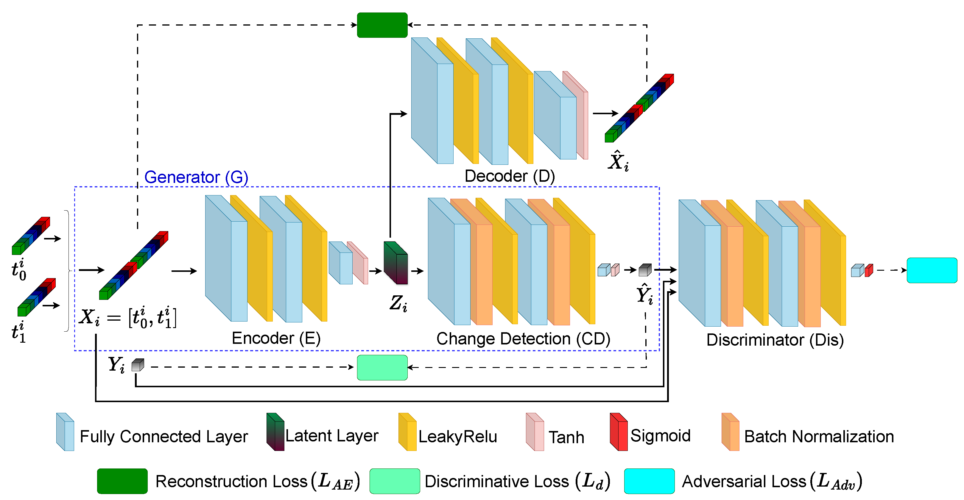
• This study proposes EFC-AdvNet, a novel end-to-end fully connected adversarial network for hyperspectral change detection. This network combines a self-spectral reconstruction (SSR) module with an adversarial change detection (Adv-CD) module to extract relevant spectral features and delineate changes between bitemporal HSIs.
• The proposed EFC-AdvNet employs an innovative joint learning by integrating the SSR module’s autoencoder for dimensionality reduction with the Adv-CD module’s change detection network. This synergy enables the direct generation of accurate change maps.
• In this study, we implement comprehensive training through a unified loss function derived from the concurrent learning of the SSR and Adv-CD modules. The experimental results on three public datasets demonstrate EFC-AdvNet’s superior performance compared with that of state-of-the-art methods.

2. Materials and Methods

2.1. Dataset Description

The HSI datasets utilized in this study’s experiments were sourced from the Earth Observing-1 (EO-1) Hyperion sensor. The EO-1 Hyperion sensor spans a spectral range of $0.4$ to $2.5$ micrometers, encompassing 242 spectral bands. It offers a spectral resolution of approximately 10 nanometers and a spatial resolution of 30 m. Despite the availability of 242 spectral bands in the Hyperion sensor, the quality of HSI data can be significantly compromised by atmospheric conditions, with certain bands exhibiting a low signal-to-noise ratio (SNR). Consequently, based on prior research and the requirements for effective image analysis visualization, only bands demonstrating a high SNR are chosen for subsequent analysis. The conducted experiments leverage these selected datasets after noise reduction and utilize ground truth maps for the purpose of binary change detection.

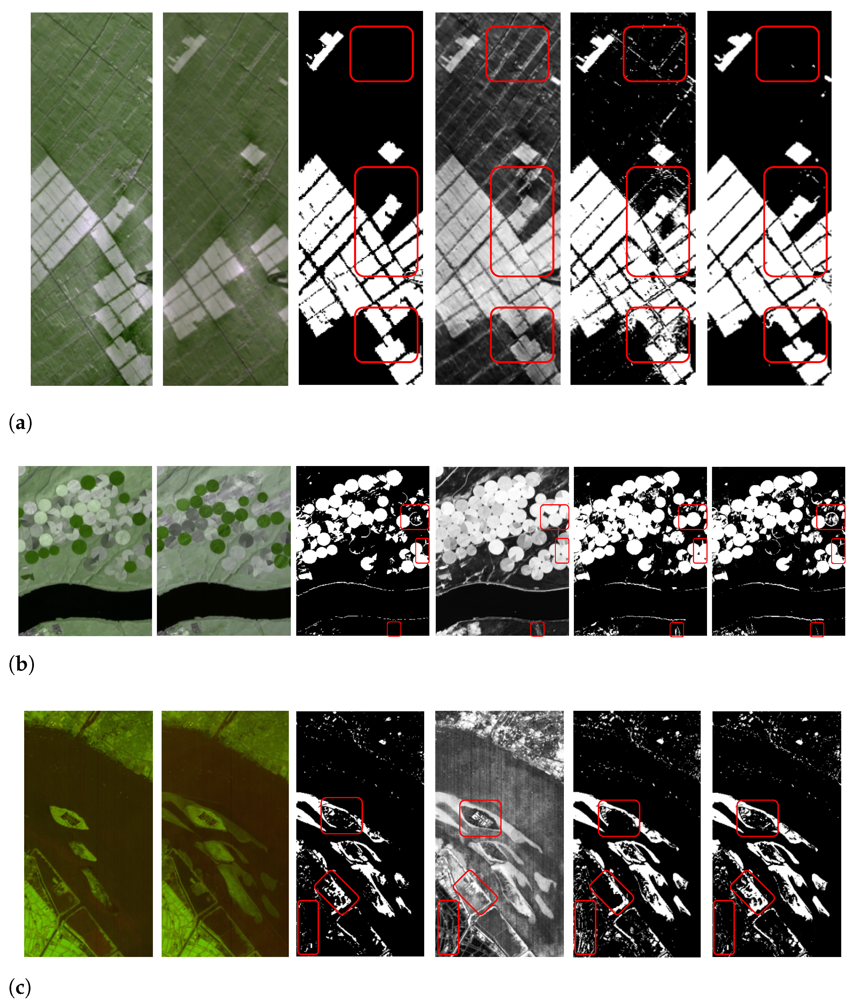
• Farmland dataset [37]: This dataset, which is also known as the China dataset, comprises bitemporal HSIs captured on 3 May 2006 ($T_0$) and 23 April 2007 ($T_1$), over farmland in Yuncheng, Jiangsu, China. These images have a size of $420\times 140$ pixels with 155 spectral bands after the removal of noisy and water-absorbing bands. It primarily focuses on changes in crops and is suitable for surveys related to changes in cultivated land. Pseudo-color images utilizing bands 91, 103, and 123 are depicted in Figure 2a.
• Hermiston dataset [38]: This dataset, which is also known as the USA dataset, originates from an irrigated agricultural area in Hermiston, located in Umatilla County, Oregon, USA. The dataset was collected on two occasions: 1 May 2004 ($T_0$) and 8 May 2007 ($T_0$). It encompasses a diverse landscape that includes a variety of irrigated fields, a river, and cultivated lands. The dataset images’ dimensions are $307\times 241$ pixels, and it includes 154 spectral bands. For visualization purposes, pseudo-color images that combine bands 91, 103, and 123 are presented in Figure 2b.
• River dataset [39]: This dataset consists of bitemporal HSIs captured on 3 May 2013 and 31 December 2013, in Jiangsu province, China. This dataset comprises images of $463\times 241$ pixels with 198 spectral bands after the removal of noisy bands. The primary focus of this dataset is on detecting the disappearance of substances in the river. Pseudo-color images that combine bands 30, 60, and 100 are presented in Figure 2c.

2.2. Methodology

In this section, we thoroughly examine our novel methodology. We begin by explaining the self-spectral reconstruction module, which is employed to reduce hyperspectral dimensions and extract spectral features. Following this, we discuss the architecture of the adversarial change detection module, a fully connected GAN that forms the foundation for reliable change detection.

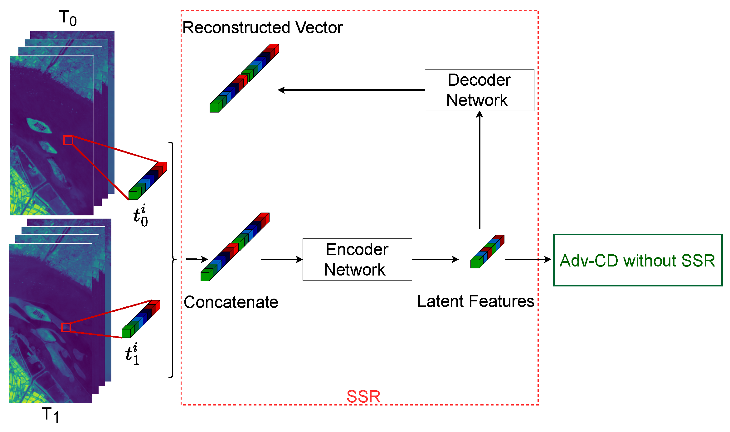
2.2.1. Self-Spectral Reconstruction (SSR)

Hyperspectral change detection encounters the challenge of the curse of dimensionality. To mitigate this issue, we propose restricting the entire latent space for characterizing HSIs to minimize reconstruction errors, thereby ensuring that latent features effectively capture the original data. Our approach involves utilizing a self-spectral reconstruction module based on an autoencoder network to extract spectral features in a low-dimensional representation by modeling the projections of observed bitemporal HSIs into the latent space.

Let $T_0$ and $T_1$ represent hyperspectral bitemporal images with $P\times Q$ as the total number of pixels and K spectral channels.

$$\begin{array}{c}{T}_0=\left[t_0^1,t_0^2,\dots ,t_0^i,\dots ,t_0^{(P\times Q)}\right]\in {\mathbb{R}}^{(P\times Q\times K)},\\ T_1=\left[t_1^1,t_1^2,\dots ,t_1^i,\dots ,t_1^{(P\times Q)}\right]\in {\mathbb{R}}^{(P\times Q\times K)},\end{array}$$

(1)

where $t_0^i$ and $t_1^i$ denote the spectral vectors of the pixel i of images acquired at $T_0$ and $T_1$, respectively. The encoder (E) learns to compress the concatenated vector $X_i$ of the bitemporal spectral vectors $t_0^i$ and $t_1^i$ to a low-dimensional representation $Z_i$ through the function f, while the decoder (D) decompresses the low-dimensional vector $Z_i$ to a reconstructed vector using the function g as follows:

$$\begin{array}{}\mathrm{(2)}& \hfill X_i& =& \left[t_0^i,t_1^i\right],\hfill \mathrm{(3)}& \hfill Z_i& =& f\left(W^e{X}_i+b^e\right),\hfill \mathrm{(4)}& \hfill {\widehat{X}}_i& =& g\left(W^d{Z}_i+b^d\right),\hfill \end{array}$$

where the encoding process is parameterized by the trainable weight matrix $W^e$ and bias vector $b^e$, while the decoding process is governed by the weight matrix $W^d$ and bias vector $b^d$ to obtain the reconstructed vector ${\widehat{X}}_i$. The mean squared error (MSE) is chosen as the loss function $L_{AE}$ to train the autoencoder. This loss function gives a higher weight to larger errors than smaller ones, which makes it suitable for image reconstruction tasks.

$$L_{AE}={\parallel X_i-{\widehat{X}}_i\parallel }_2^2.$$

(5)

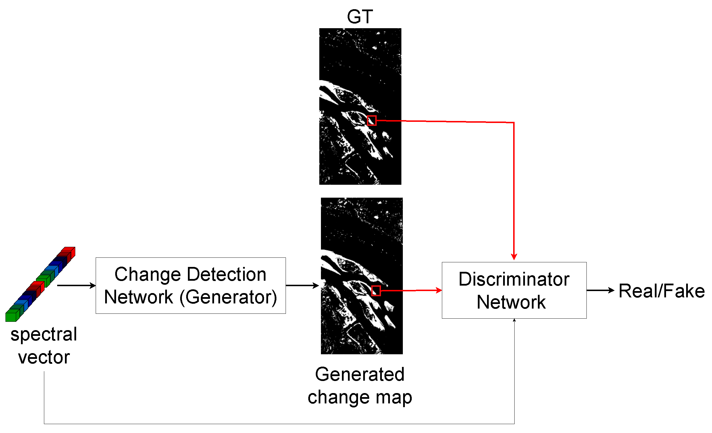
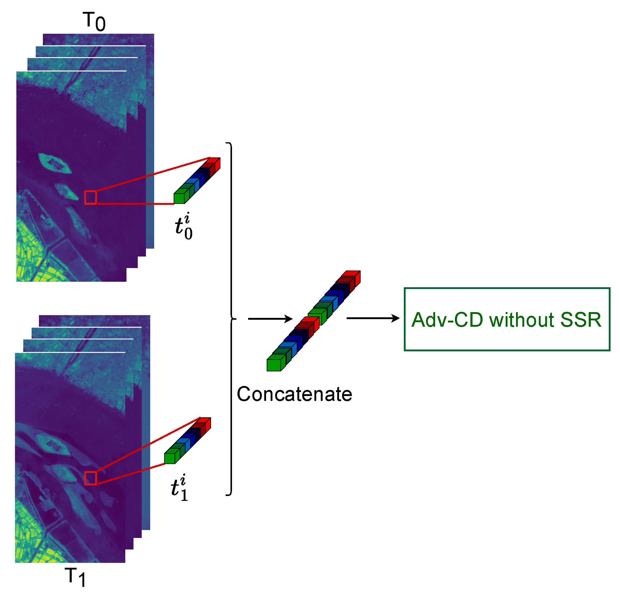
2.2.2. Adversarial Change Detection (Adv-CD) for Hyperspectral Images

In order to detect changes from a low-dimensional representation of bitemporal HSIs, the generated spectral vector $Z_i$ from the encoder network of the SSR module is fed into a change detection network ($CD$). The encoder network and the change detection network are combined and trained together as a generator (G) that is part of the Adv-CD module, as shown in Figure 1. The main function of the generator is to map the bitemporal hyperspectral vectors into a changed or unchanged pixel through the function C, which is defined as follows:

$${\widehat{Y}}_i=C\left(W^c·f\left(W^e{X}_i+b^e\right)+b^c\right),$$

(6)

where $W^c$ and $b^c$ are the trainable parameters of the change detection network. All of the parameters of the encoder and the CD network are updated while training the generator to detect changes from the bitemporal HSIs. The result is then fed into the discriminator ($Dis$) to decide whether the generated pixel ${\widehat{Y}}_i$ is correct or not based on the pixels of the real ground truth (GT) image. The generator and the discriminator sub-networks are trained in an adversarial manner, where the generator undertakes the responsibility of translating the combined vector $X_i$ into a changed or unchanged pixel. Simultaneously, the discriminator is given the combined input vector $X_i$ and a real or generated pixel and must determine whether the generated pixel is real or fake. Therefore, the generator and the discriminator are trained in an adversarial manner where the generator tries to fool the discriminator by generating pixels as correctly as possible, and the discriminator tries to distinguish between the generated and real pixels through the following adversarial loss:

$$L_{Adv}(G,Dis)=Argmi{n}_{G}ma{x}_{Dis}L\left(G,Dis\right),$$

(7)

where L is the commonly used loss function of the conditional GAN [40] defined as follows:

$$L={\mathbb{E}}_{(X,Y)}\left[log\left(Dis\right(X,Y\left)\right)\right]+{\mathbb{E}}_X\left[log\left(1-Dis(X,G(X\left)\right)\right)\right].$$

(8)

The generation of the output is conditioned on the bitemporal vectors. The discriminator is provided both with bitemporal images and with the change map. The discriminator is updated directly, while the generator is updated indirectly through the discriminator, with the loss function being updated accordingly. The generator is trained using an adversarial loss, which encourages the generator to produce realistic pixel values. The generator is also updated via discriminative loss $L_d$, which is measured between the generated pixel ${\widehat{Y}}_i$ and the expected output pixel $Y_i$ extracted from the real change map. It is expressed as follows:

$$L_d=|Y_i-{\widehat{Y}}_i|.$$

(9)

This additional loss encourages the generator to create plausible translations of the input images. We chose the mean absolute error (MAE), which is often more interpretable than the MSE because it is on the same scale as the original data and can compare the pixel intensity values, making it more suitable for our case. The weights of the generator are updated using a combination of the adversarial loss ($L_{Adv}$), which is derived from the discriminator output, and the discriminative loss ($L_d$). These two loss scores are added together, with the loss $L_d$ serving as a regularizing term, and this is weighted by a hyperparameter denoted as alpha ($\alpha$). According to the originally proposed loss function in [40], this parameter is set to 100 in order to give the $L_d$ loss more importance than the adversarial loss for the generator during training. The GAN loss can be expressed as follows:

$$L_{GAN}=L_{Adv}+\alpha L_d.$$

(10)

The encoder network, a pivotal component shared between the generator sub-network and the SSR module, is updated through the global loss ($L_G$), which combines the GAN loss ($L_{GAN}$) and reconstruction loss ($L_{AE}$), as presented in the following equation:

$$L_G=L_{GAN}+\beta L_{AE},$$

(11)

where $L_{AE}$ is weighted by $\beta$, which is set to 1. According to the experiment, it is found that maintaining equal weights for both the GAN loss ($L_{GAN}$) and the reconstruction loss ($L_{AE}$) yielded the best performance. This approach ensures that neither loss dominates the optimization process, allowing the model to effectively learn from both aspects.

2.2.3. Network Architecture 

In the training process, each pixel in the spatial domain, corresponding to a spectral vector, is treated as an individual training sample. The training batch size is set to be equal to the total number of spatial pixels present in the given HSI. A fully connected network architecture is chosen to effectively handle vector inputs by connecting every input neuron to every output neuron, allowing for complex interactions between input features. The network architecture utilized consists of four layers (input, two middle layers, and output). The units in the different components are defined as follows: E {$2K,500,500,S$}, D {$S,500,500,2K$}, $CD$ {$S,500,500,1$}, and $Dis$ {$1+2K,500,500,1$} for the encoder, decoder, change detection network, and discriminator, respectively. The number of hidden units S in the deep latent layer is initially constrained to $\sqrt{K}+1$ based on the findings of [41]. Subsequent experiments are conducted to determine the optimal number of representative bands for improved change detection performance, as depicted in Section 3.3.

All fully connected layers in the SSR module, change detection network, and discriminator employ the $LeakyReLU$ activation function (slope $0.2$), while the final layer of the encoder, decoder, and change detection network uses the $tanh$ activation function. The last layer of the discriminator utilizes the $sigmoid$ activation function, as depicted in Figure 3. In deep neural networks, managing parameter changes and training complexity can lead to internal covariate shift issues. To address this challenge, batch normalization (BN) is implemented to standardize activations from preceding layers to achieve zero mean and unit variance. This normalization technique stabilizes the training process. Therefore, BN is applied before LeakyReLU activation in both the change detection and discriminator networks to ensure consistent activation with stable distribution and to expedite training efficiency. The BN is expressed as follows:

$$BN\left(x\right)={\displaystyle \frac{x-E\left(x\right)}{\sqrt{\mathrm{var}\left[x\right]+ϵ}}},$$

(12)

where $E\left(x\right)$ and $var\left[x\right]$ denote the mean and variance of a mini-batch, respectively. To prevent division by zero, $ϵ$ is set to ${10}^{-8}$. Additionally, x refers to the input of each fully connected layer within our architecture.

3. Experiments and Results

3.1. Experimental Setup

The proposed EFC-AdvNet was developed using TensorFlow v2.11.0 and implemented on a single NVIDIA RTX 3090 GPU, which is manufactured by Yunxuan Ltd. from Shanghai, China.We trained all components of the network using a stochastic Adam optimizer, setting the learning rate to 0.001 for the SSR component and 0.0001 for the discriminator. The training process was concluded after 100 epochs. Given that our approach is pixel-based, we randomly selected about 10% from the total number of pixels from each dataset to be used for training and validation. With this number of pixels, we obtain a substantial number of training samples. For instance, as indicated in

Table 1. Pixel count and distribution for each dataset.

Dataset	Total Pixels	Changed Pixels	Unchanged Pixels	Selected Pixels
Farmland	58,800	18,383	40,417	5800
Hermiston	73,987	16,676	57,311	7000
River	111,583	9698	101,885	10,000

, using 10% from the River dataset yields approximately 10,000 samples. This is a significant amount of data for training purposes, allowing the model to learn effectively despite the relatively small percentage of pixels used. The batch size used for training is set to 256.

3.2. Evaluation

The evaluation of our change detection framework included the utilization of two key assessment metrics: the overall accuracy ($OA$) and $Kappa$ coefficient.

$$\begin{array}{ccc}\hfill OA& =& {\displaystyle \frac{TP+TN}{N}}\times 100(\%),\hfill \end{array}$$

(13)

$$\begin{array}{ccc}\hfill Kappa& =& {\displaystyle \frac{OA-P}{1-P}}\times 100(\%),\hfill \end{array}$$

(14)

with

$$P={\displaystyle \frac{(TP+FP)(TP+FN)}{N^2}}+{\displaystyle \frac{(FN+TN)(FP+TN)}{N^2}},$$

(15)

where $TP$, $FP$, $TN$, $FN$, and N correspond to the counts of true positives, false positives, true negatives, false negatives, and the total number of pixels, respectively. These metrics collectively provided a comprehensive understanding of the framework’s performance.

In change detection, $OA$ provides a general measure of the algorithm’s ability to accurately detect changes and non-changes across an entire dataset. The $Kappa$ coefficient provides a more nuanced understanding of the algorithm’s performance by considering that the agreement that could happen by chance, offering a complement to the $OA$ metric. High values of these two metrics mean better results.

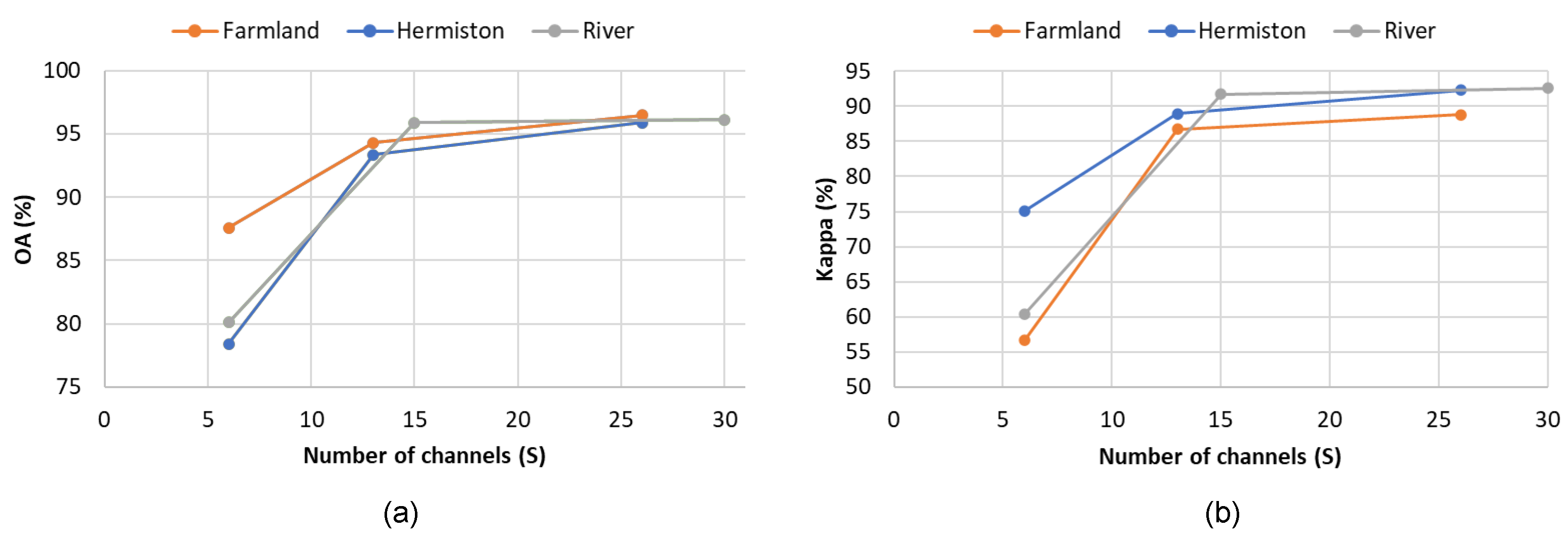
3.3. Tuning the Number of Channels in the Latent Feature Space 

As depicted in Section 2.2.3, the optimal number of channels S in the latent space for compressing the hyperspectral data, according to [41], is $\sqrt{K}+1$, where K is the number of input channels of an HSI. In practice, to determine this optimal number of channels in the latent feature space for a low-dimensional representation of bitemporal hyperspectral data, a series of experiments were conducted. For each dataset, we varied the number of channels among six channels, $\sqrt{K}+1$, and $2(\sqrt{K}+1)$, and our network underwent training and was subsequently evaluated using validation data. The final choice of the number of channels is based on the best performance of EFC-AdvNet for each dataset. The outcomes are detailed in

Table 2. EFC-AdvNet’s performance with the number of channels (S) of the latent feature space for the three datasets. The highest metrics values in each dataset are marked in bold.

Dataset	Number of Channels (S)	$\mathit{OA}$  $(\%)$	$\mathit{Kappa}$  $(\%)$
Farmland (K = 155)	$S=6$	78.40	56.76
	$S=\sqrt{K}+1=13$	93.37	86.74
	$S=2(\sqrt{K}+1)=26$	95.91	88.82
Hermiston (K = 154)	$S=6$	87.57	75.12
	$S=\sqrt{K}+1=13$	94.32	88.92
	$S=2(\sqrt{K}+1)=26$	96.51	92.31
River (K = 198)	$S=6$	80.10	60.46
	$S=\sqrt{K}+1=15$	95.88	91.75
	$S=2(\sqrt{K}+1)=30$	96.14	92.57

.

The results presented in Figure 4 indicate that reducing the number of channels to six results in the lowest values for both the overall accuracy ($OA$) and $Kappa$ metrics across all three datasets. This reduction leads to instability in the EFC-AdvNet, as it struggles to learn effectively from such low-dimensional representations of bi-temporal HSIs. Consequently, the network’s ability to detect changes between images is compromised, resulting in a significant increase in false change detections. Based on these findings, the optimal number of channels was determined to be $S=2(\sqrt{K}+1)$ for all three datasets. This conclusion is supported by the higher values of the overall accuracy $OA$ and $Kappa$ metrics compared to those obtained with $S=\sqrt{K}+1$, as shown in Figure 4 and further detailed in Table 2.

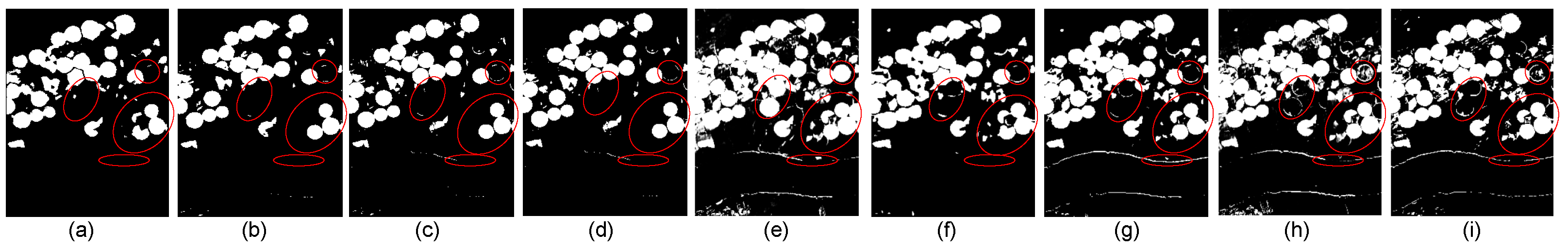
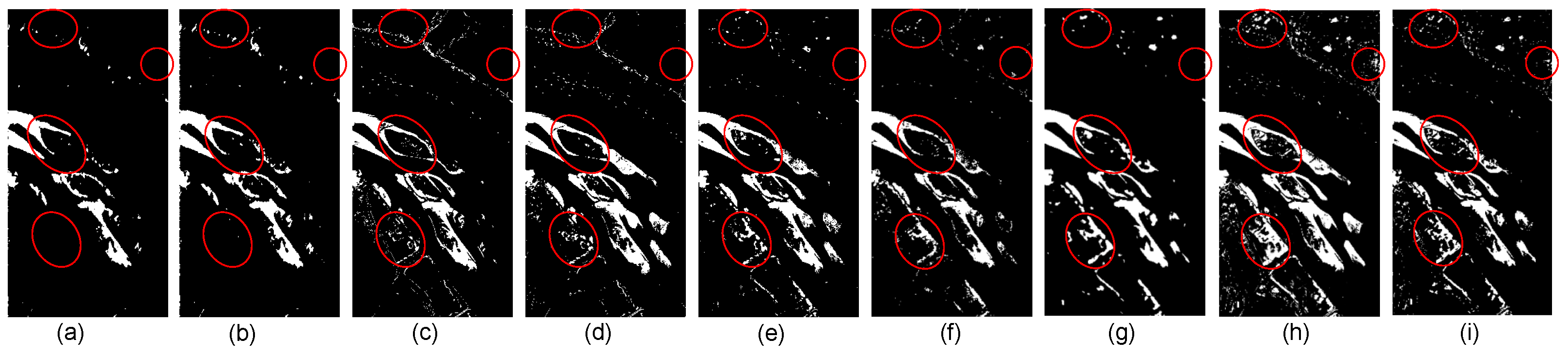
3.4. Comparison with State-of-the-Art Change Detection Methods in Hyperspectral Imaging

To comprehensively assess the performance of the proposed change detection network for HSIs, we conducted both quantitative and qualitative comparisons against several state-of-the-art (SOTA) change detection methods. These SOTA methods were selected as benchmarks to measure the efficacy of our method. The specific SOTA methods included in this evaluation are as follows:

• Change vector analysis (CVA) [42]: CVA leverages spectral feature vectors from corresponding spatial positions in two images, representing spectral change vectors in polar coordinates with the magnitude and direction. Carvalho et al. introduced the spectral angle mapper (SAM) and spectral correlation mapper (SCM) to enhance the direction calculation in CVA.
• Anomaly change detection (ACD) [13]: ACD employs autoencoders to detect complex spectral differences in multitemporal HSIs. Siamese autoencoder networks construct predictors from different directions to model spectral variations, generating loss maps that highlight anomaly changes while suppressing unchanged pixel differences.
• General end-to-end 2D CNN (GETNET) [39]: GETNET introduces an end-to-end 2D convolutional neural network tailored for hyperspectral change detection tasks. It overcomes data limitations and the underutilization of deep learning features by utilizing a mixed-affinity matrix to capture changed patterns and enhance cross-channel gradient information.
• Self-supervised hyperspectral spatial–spectral feature understanding network (HyperNet) [43]: HyperNet integrates spatial and spectral attention branches to extract discriminative spatial and spectral information independently, and it merges them to generate comprehensive features. Trained using a self-supervised learning framework, HyperNet achieves pixel-level feature learning through similarity comparisons of multitemporal HSIs.
• Spectral–spatial–temporal transformers for hyperspectral image change detection (SST-Former) [11]: The SST-Former encodes each pixel to capture spectral and spatial sequences, employs a spectral transformer encoder for spectral information extraction, and utilizes a spatial transformer encoder for texture information.
• Spectral–temporal transformer for hyperspectral image change detection (STT) [10]: STT processes the HSI CD task from a sequential perspective by concatenating feature embeddings in spectral order, establishing a global spectrum–time-receptive field. Through a multi-head self-attention mechanism, the STT effectively captures spectral–temporal features.
• End-to-end cross-band 2D attention network for hyperspectral change detection (CBANet) [44]: By integrating a cross-band feature extraction module with a 2D spatial–spectral self-attention module, CBANet effectively extracts spectral differences between matching pixels while considering the correlation between adjacent pixels in remote sensing.

In assessing the impact of our approach, we conducted a comprehensive comparison with established methods, examining both visual and qualitative aspects. Detailed $OA$ and $Kappa$ statistics for the three datasets are presented in

Table 3. Comparison of the performance of the SOTA methods against our proposed EFC-AdvNet on the three datasets. The highest metrics values in each dataset are marked in bold.

Methods	Farmland		Hemiston		River
	$\mathit{OA}$  $(\%)$	$\mathit{Kappa}$  $(\%)$	$\mathit{OA}$  $(\%)$	$\mathit{Kappa}$  $(\%)$	$\mathit{OA}$  $(\%)$	$\mathit{Kappa}$  $(\%)$
CVA	92.43	78.08	92.21	76.67	93.87	77.93
ACD	94.23	78.55	92.72	76.70	94.29	78.67
GETNET	94.63	85.72	94.31	77.25	95.14	76.39
HyperNet	93.98	80.01	92.66	76.93	95.59	80.46
SST-Former	95.05	87.52	95.36	90.73	95.79	91.26
STT	94.84	87.98	97.03	90.36	96.74	84.93
CBANet	95.26	88.10	96.68	91.57	97.12	85.36
EFC-AdvNet	95.91	88.82	96.51	92.31	96.14	92.57

. Additionally, Figure 5, Figure 6 and Figure 7 showcase the visual results for the Farmland, Hermiston, and River datasets, respectively, providing a clear illustration of the effectiveness of our method.

The analysis of the results for the Farmland dataset reveals varying performance among the different methods. The CVA method achieved the lowest $OA$ and $Kappa$ values. ACD exhibited improvement over CVA, achieving an $OA$ value of 94.23% and a $Kappa$ value of 78.55%, indicating its enhanced accuracy in change identification, as depicted in Figure 5. HyperNet also showed improvement, with an $OA$ value of 93.98% and a $Kappa$ value of 80.01%. Visual interpretation suggests the presence of more false positives (i.e., pixels that are actually unchanged but detected as changed) in HyperNet’s results compared with the GETNET method. GETNET had notably improved performance, with a $Kappa$ value of 85.72%. The change detection transformer methods, SST-Former and STT, demonstrated superior performance compared to previous approaches, showcasing competitive results between the two. CBANet, which uses a self-attention module, also exhibited competitive performance with our method, achieving an $OA$ value of 95.26%. However, our method outperformed all other models, attaining the highest $OA$ and $Kappa$ values of 88.82% and 95.91%, respectively. This indicates the effectiveness of employing adversarial learning in change detection compared to other techniques. In Figure 5, our method, SST-Former, STT, and CBANet demonstrate reduced false positives compared with HyperNet and ACD. However, there are instances of misclassification where unchanged areas are incorrectly identified as changed areas. Based on visual interpretation, our method outperforms SST-Former, STT, and CBANet methods in accurately delineating changed areas, clearly establishing the effectiveness of our approach.

For the Hermiston dataset, the STT method achieved the highest overall accuracy of 97.03%, outperforming all other methods. However, it exhibited a lower Kappa value compared to SST-Former and CBANet, while our method achieved the highest $Kappa$ value of 92.31%. It is important to note that while overall accuracy provides a straightforward measure of model performance, it can be misleading, particularly in cases where class distribution is imbalanced. The Hermiston dataset is considered imbalanced relative to the Farmland dataset; as shown in Table 1, the changed class comprises only 22.54% (16,676 changed pixels) of the total number of pixels, compared to 77.46% (57,311 unchanged pixels) for the unchanged class. In this context, the STT model may predominantly predict the majority class, thus achieving high accuracy even if it fails to identify any instances of the minority class. The visual comparison presented in Figure 6 demonstrates that STT exhibited some missed detections when compared with our proposed method, EFC-AdvNet, which showcases superior performance. This further emphasizes the advantages of our approach in accurately detecting changes within imbalanced datasets.

In the case of the River dataset, which is highly imbalanced with only 8.69% of the changed class, the SST-Former method slightly surpassed both GETNET and HyperNet in overall accuracy. It also demonstrated a notable improvement in Kappa compared to the ACD, CVA, STT, and CBANet methods. Our method, on the other hand, outperformed all SOTA methods, achieving a $Kappa$ value of 92.57%, which is nearly 7.21% higher than that of CBANet, which recorded the highest OA of 97.12%. In this highly imbalanced dataset, $Kappa$ is particularly valuable for evaluating model performance because it provides a more nuanced perspective by accounting for agreement beyond what would be expected by chance. While overall accuracy offers a general sense of performance, $Kappa$ delivers deeper insights into how effectively a model performs across different classes, especially in imbalanced scenarios. The visual results presented in Figure 7 indicate that our model provided more precise detection, demonstrating the effectiveness of the joint learning between the SSR module and the adversarial learning module. This joint learning approach significantly aids in addressing the challenges posed by imbalanced class distributions.

Our proposed method demonstrates several key advantages over other state-of-the-art hyperspectral change detection techniques. Firstly, it achieves the highest $Kappa$ value across multiple datasets, indicating a more reliable change detection capability. The use of the SSR module for dimensionality reduction helps efficiently process the inherently high-dimensional hyperspectral data, allowing the Adv-CD module to focus on the most relevant features and enhance performance. Notably, the method exhibits consistent state-of-the-art or competitive performance across different datasets, such as the Farmland, Hermiston, and River datasets, showcasing its robustness and adaptability to various types of hyperspectral imagery. The high $Kappa$ scores further suggest excellent agreement between the predicted change map and the ground truth, which is crucial for applications requiring precise change detection. Furthermore, the proposed EFC-AdvNet outperforms traditional methods such as CVA; deep learning baselines such as ACD, GETNET, and HyperNet; and transformer-based methods such as SST-Former. This underscores the effectiveness of combining the Adv-CD and SSR modules for hyperspectral change detection.

3.5. Ablation Study on the SSR Module

In this section, our focus is on training and evaluating the proposed change detection network in two configurations involving the SSR module to highlight its impact on detecting changes in HSIs. The Adv-CD in these experiments is composed of a change detection network, which serves as the generator, and a discriminator network, as presented in Figure 8. In the first configuration without the SSR module, we train the Adv-CD without incorporating the SSR module. The model processes bitemporal hyperspectral input images and generates a change map directly from the high-dimensional concatenated vector, as depicted in Figure 9. Moving to the second configuration with separate training of the SSR module and the Adv-CD module, as depicted in Figure 10, we initially train the SSR module independently from the change detection module until it stabilizes. Subsequently, the predicted latent feature vector is inputted into the change detection network, serving as the generator component of the Adv-CD, to produce the change map.

Table 4. Comparison of model performance in different training configurations for the SSR module across the three datasets. The highest metrics values in each dataset are marked in bold.

Dataset	Configuration	$\mathit{OA}$  $(\%)$	$\mathit{Kappa}$  $(\%)$
Farmland	Without SSR	81.46	62.89
	Separate SSR and Adv-CD	90.47	80.95
	SSR+Adv-CD (EFC-AdvNet)	95.91	88.82
Hermiston	Without SSR	71.22	42.40
	Separate SSR and Adv-CD	86.08	72.17
	SSR+Adv-CD (EFC-AdvNet)	96.51	92.31
River	Without SSR	51.16	37.98
	Separate SSR and Adv-CD	88.62	77.25
	SSR+Adv-CD (EFC-AdvNet)	96.14	92.57

and Figure 11 present the quantitative and qualitative comparative results for different training configurations of the proposed network. The evaluation metrics in the table and the visual comparisons in the figure clearly indicate that training the Adv-CD without the SSR module results in lower detection performance than that of configurations where the SSR module is utilized. Integrating the SSR module yields higher $OA$ and $Kappa$ values than those of the previous setup. However, visual inspection reveals that the second configuration produces numerous false positives, where unchanged pixels are misclassified as changed, leading to low detection precision across all datasets.

Simultaneous training of the SSR module with the change detection module as in our EFC-AdvNet enhances the performance of change detection compared with previous configurations. The high $Kappa$ value means that the proposed configuration is very accurate in its predictions, with a low rate of false positives. Moreover, the high $OA$ value indicates that the EFC-AdvNet configuration is able to identify most of the relevant changes within the three datasets, as shown in Figure 11. This approach results in the highest change detection accuracy among all configurations.

To further elucidate the impact of combined training of the SSR and Adv-CD module on spectral vector reconstruction, we randomly select spectra at times $T_0$ and $T_1$ from the reconstructed HSIs of the SSR module when trained separately and jointly with the Adv-CD. As depicted in Figure 12, the dashed green curve representing combined training more closely aligns with the original input spectral vector than the blue dashed curve. These experimental results demonstrate that, in contrast to separate training, combined training enhances the encoder’s ability to characterize high-dimensional spectral images in the deep latent space, preserving more spectral information in hidden features. The integration of the SSR module and adversarial learning during change detection proves more advantageous for subsequent change detection within the network while reducing the dimensionality of input HS images. This synergy not only improves change detection accuracy but also positively impacts spectral vector reconstruction.

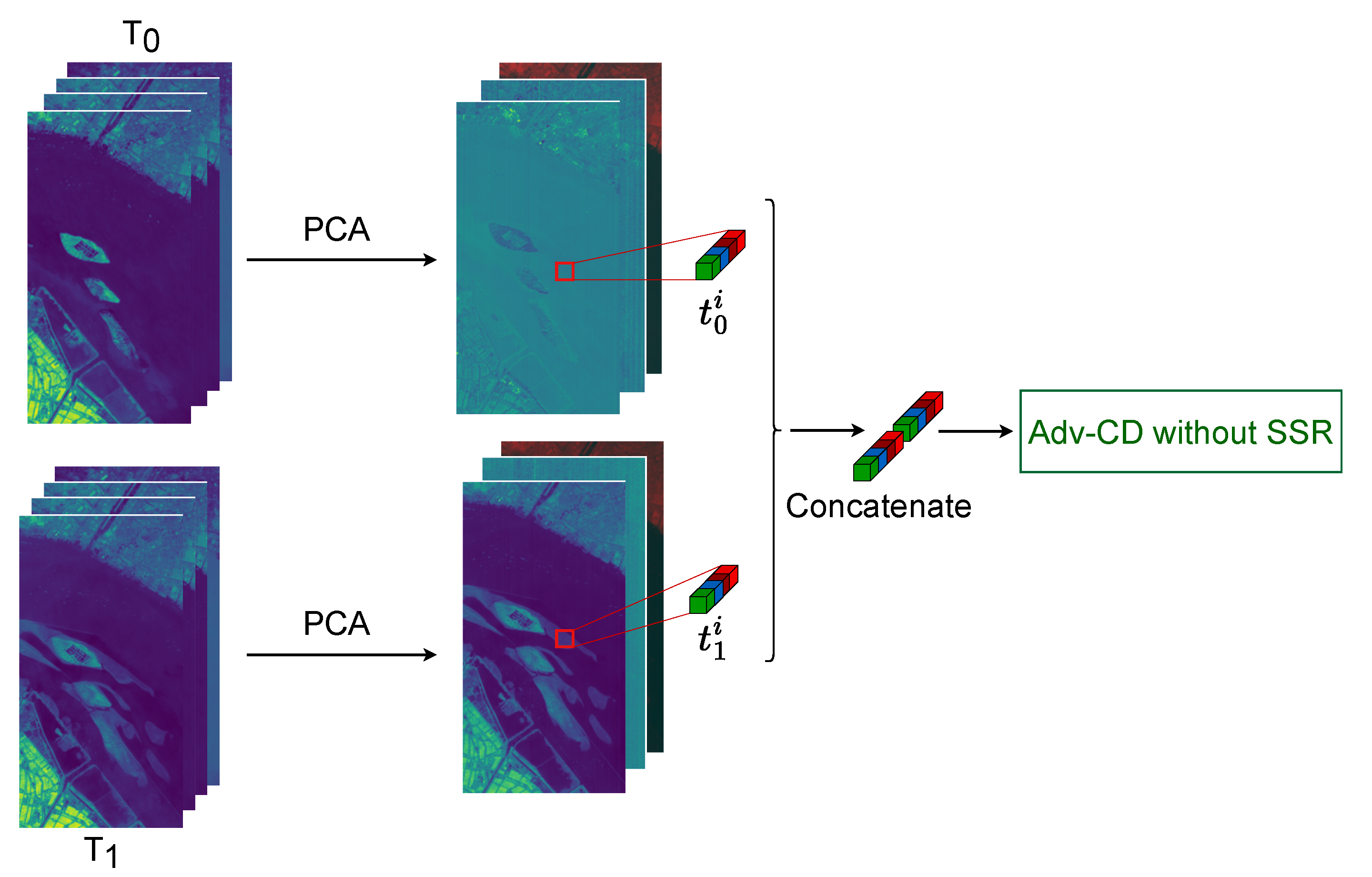
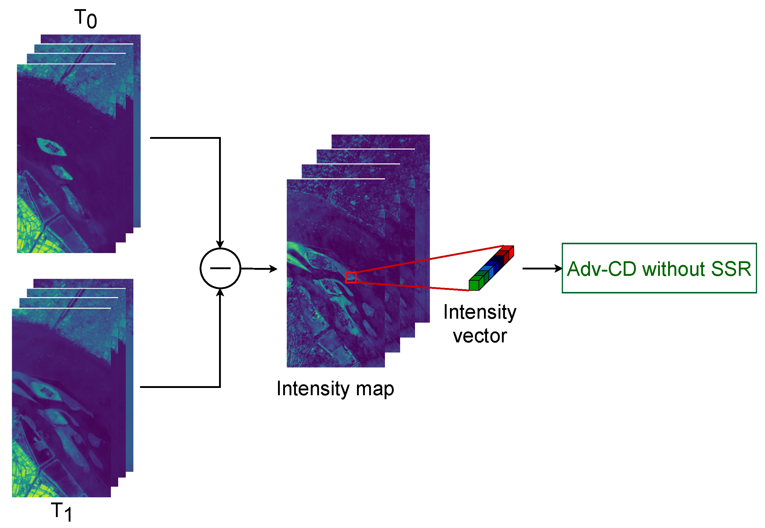
3.6. Comparative Analysis of Various Spectral Representation Methods

In the preceding section, we established the necessity of the SSR module for accurate spectral feature extraction in change detection. This section focuses on integrating various spectral representations of bitemporal images into the change detection process. Our objective is to explore two preprocessing techniques for bitemporal HSIs before inputting them into the Adv-CD module for change detection.

The first preprocessing technique, as shown in Figure 13, involves using PCA for dimensionality reduction. PCA is applied to each hyperspectral image to obtain a low-dimensional image with $2(\sqrt{K}+1)$ channels. These resulting images are then utilized in the Adv-CD module illustrated in Figure 8. The second preprocessing technique, as illustrated in Figure 14, entails calculating the absolute difference between the bitemporal HSIs, and the resulting intensity image is subsequently fed into the Adv-CD presented in Figure 8. Ultimately, we compare these preprocessing methods with the proposed EFC-AdvNet for dimensionality reduction and change detection, aiming to evaluate their effectiveness in enhancing the change detection process.

Table 5. Quantitative comparison of using PCA, image differencing, and the SSR module. The highest metrics values in each dataset are marked in bold.

Dataset	Configuration	$\mathit{OA}$  $(\%)$	$\mathit{Kappa}$  $(\%)$
Farmland	PCA+Adv-CD	72.45	44.81
	Intensity+Adv-CD	92.52	85.03
	SSR+Adv-CD (EFC-AdvNet)	95.91	88.82
Hermiston	PCA+Adv-CD	82.43	64.86
	Intensity+Adv-CD	95.14	90.27
	SSR+Adv-CD (EFC-AdvNet)	96.51	92.31
River	PCA+Adv-CD	77.15	54.59
	Intensity+Adv-CD	95.25	90.50
	SSR+Adv-CD (EFC-AdvNet)	96.14	92.57

displays the performance of different training configurations (PCA+Adv-CD, Intensity+Adv-CD, SSR+Adv-CD) applied to the three datasets; this was assessed with two metrics: $OA$ and $Kappa$. Among these configurations, PCA+Adv-CD exhibits the lowest performance across all datasets. Intensity+Adv-CD demonstrates a notable improvement compared with the previous configuration for all datasets. On the other hand, SSR+Adv-CD (EFC-AdvNet) showcases the best performance, with superior values across all metrics. Observing Figure 15, a slight visual similarity is evident in the resulting change maps from the Intensity+Adv-CD and SSR+Adv-CD configurations. However, SSR+Adv-CD, the proposed EFC-AdvNet, displays greater robustness against false detections than that of Intensity+Adv-CD, as reflected in the highest $OA$ and $Kappa$ values in Table 5.

4. Discussion

According to the results presented here, the exceptional performance of EFC-AdvNet across all three datasets, with the highest $OA$ and $Kappa$ values in comparison with other SOTA methods, highlights its ability to accurately and reliably detect changes in HSIs by effectively capturing subtle spectral changes and aligning with ground truth data. This high performance is due to the combination of the SSR module with the Adv-CD module. The use of the SSR module for dimensionality reduction and the dependent learning of the encoder part of this module on the training of the Adv-CD module for change detection contribute significantly to the performance of our change detection framework through several key mechanisms:

• Feature selection and noise reduction: The encoder part of the SSR module effectively learns compressed representations of the data by encoding the most relevant features while discarding noise and redundant information. This process of dimensionality reduction helps isolate the essential features that are critical for detecting changes in HSIs, thereby improving the ability of the Adv-CD module to focus on significant differences between images.
• Improved generalization: The compressed representation learned by the SSR module can help the change detection model based on adversarial learning generalize better to unseen data by focusing on the underlying patterns and features that are most relevant for change detection. This can enhance EFC-AdvNet’s robustness and its ability to accurately detect changes across different environments and conditions.
• Enhanced learning capability: The resulting latent feature space from the encoder facilitates the learning process of the Adv-CD module by providing a more structured and simplified input space. This led to better convergence during training and improved performance in detecting subtle changes that might be missed in the high-dimensional raw data.
• Complexity: The total number of parameters in our model is approximately 4.45 MB for the River dataset, which has the highest number of channels among the datasets used. This relatively low parameter count indicates that our model is not overly complex. This simplicity enables efficient execution even on systems without dedicated GPU support. Moreover, our method employs a pixel-based approach, where the input is represented as a 1D vector. This design choice further simplifies the computations required, making them less resource-intensive than object-based methods. Object-based approaches often necessitate more complex processing due to their reliance on spatial relationships and larger input sizes, which can increase computational demands. Consequently, our model offers an efficient solution for hyperspectral change detection, making it accessible for a wider range of applications and hardware configurations.

Furthermore, dimensionality reduction using the SSR module offers several key advantages over traditional methods such as PCA and image differencing for generating intensity maps in change detection for HSIs. The SSR module’s autoencoder architecture can capture nonlinear relationships in the data, allowing it to learn more complex patterns and features than the linear PCA technique. Unlike PCA, which projects data onto axes that maximize variance without considering the task-specific relevance, the SSR module learns to encode data into a lower-dimensional space in a way that is optimized for reconstruction, which can be more useful for change detection tasks. Moreover, the SSR module is designed to be robust to noise in the data, effectively filtering out noise and focusing on the underlying signal, which is crucial for accurately detecting changes. When compared with image differencing, which simply subtracts one image from another to highlight changes, the SSR module can provide a more nuanced understanding of changes. The union of its encoder part with the change detection network can identify patterns of change that are not immediately apparent from raw intensity differences, leading to more accurate and meaningful change detection results.

In summary, the integration of the SSR module with the Adv-CD module based on adversarial learning is a key factor in the success of our approach. The SSR module’s ability to extract relevant spectral features and effectively reduce the dimensionality of the input data plays a crucial role in aiding the Adv-CD module to accurately identify changes between bitemporal HSIs. This configuration, where the encoder part of the SSR module is trained concurrently with the Adv-CD module, allows for optimal feature extraction and facilitates accurate change detection and spectral vector reconstruction. Furthermore, the combination of the SSR module with the Adv-CD module to obtain the proposed EFC-AdvNet offers advantages in terms of nonlinearity, feature learning, flexibility, and robustness to noise, making it a powerful network for extracting meaningful information from HSIs and improving the accuracy of detecting changes.

5. Conclusions

This study proposes a novel end-to-end fully connected adversarial network (EFC-AdvNet) for binary change detection in hyperspectral images. The EFC-AdvNet network comprises two interconnected deep learning modules: a self-spectral reconstruction (SSR) module and an adversarial change detection (Adv-CD) module. The SSR module employs an autoencoder network to extract relevant spectral features from the bitemporal hyperspectral imagery while simultaneously reducing their dimensionality. Crucially, the encoder part of the SSR module serves as the key subnetwork of the generator component within the Adv-CD module. It connects the two modules together, which enables the Adv-CD module to detect changes directly from the resulting low-dimensional spectral feature representation of the bitemporal HSI. This proposed EFC-AdvNet has several advantages, including the ability to capture nonlinear relationships, effective feature learning, enhanced flexibility, and improved robustness to noise. These characteristics make the proposed network a powerful tool for extracting meaningful information from hyperspectral images and improving the accuracy of binary change detection.

The experimental results demonstrate that the proposed method exhibits competitive performance compared with state-of-the-art (SOTA) techniques across three public hyperspectral datasets. However, a significant challenge remains in the reliance on supervised learning, which necessitates a substantial amount of labeled data. This requirement is particularly difficult to fulfill in hyperspectral imaging scenarios, where acquiring labeled datasets can be both time-consuming and resource-intensive. To address this limitation, future research will focus on enhancing the network architecture by exploring self-supervised training approaches. These methods have the potential to leverage the abundant unlabeled data available in hyperspectral images, thereby mitigating the challenges posed by limited labeled datasets in hyperspectral change detection. Additionally, incorporating active learning strategies could further optimize the labeling process by selectively querying the most informative samples. Moreover, spectral–spatial integration should be considered in future works to further enhance the model’s performance in detecting changes.

References

1. Alegavi, S.; Sedamkar, R. Research Trends in Hyperspectral Imagery Data. Int. J. Comput. Eng. Technol. 2019, 10, 67–73. [Google Scholar] [CrossRef]
2. Hasanlou, M.; Seydi, S.T. Hyperspectral Change Detection: An Experimental Comparative Study. Int. J. Remote Sens. 2018, 39, 7029–7083. [Google Scholar] [CrossRef]
3. Zhu, Q.; Guo, X.; Li, Z.; Li, D. A review of multi-class change detection for satellite remote sensing imagery. Geo-Spat. Inf. Sci. 2022, 27, 1–15. [Google Scholar] [CrossRef]
4. Bovolo, F.; Bruzzone, L. A Theoretical Framework for Unsupervised Change Detection Based on Change Vector Analysis in the Polar Domain. IEEE Trans. Geosci. Remote Sens. 2007, 45, 218–236. [Google Scholar] [CrossRef]
5. Deng, J.S.; Wang, K.; Deng, Y.H.; Qi, G.J. PCA-based Land-use Change Detection and Analysis Using Multitemporal and Multisensor Satellite Data. Int. J. Remote Sens. 2008, 29, 4823–4838. [Google Scholar] [CrossRef]
6. Nielsen, A.A. The Regularized Iteratively Reweighted MAD Method for Change Detection in Multi- and Hyperspectral Data. IEEE Trans. Image Process. 2007, 16, 463–478. [Google Scholar] [CrossRef] [PubMed]
7. Krinidis, S.; Chatzis, V. A Robust Fuzzy Local Information C-Means Clustering Algorithm. IEEE Trans. Image Process. 2010, 19, 1328–1337. [Google Scholar] [CrossRef]
8. Yu, S.; Tao, C.; Zhang, G.; Xuan, Y.; Wang, X. Remote Sensing Image Change Detection Based on Deep Learning: Multi-Level Feature Cross-Fusion with 3D-Convolutional Neural Networks. Appl. Sci. 2024, 14, 6269. [Google Scholar] [CrossRef]
9. Shammi, S.A.; Du, Q. Hyperspectral Image Change Detection Using Deep Learning and Band Expansion. In Proceedings of the 12th Workshop on Hyperspectral Imaging and Signal Processing: Evolution in Remote Sensing (WHISPERS), Rome, Italy, 13–16 September 2022. [Google Scholar] [CrossRef]
10. Li, X.; Ding, J. Spectral-Temporal Transformer for Hyperspectral Image Change Detection. Remote Sens. 2023, 15, 3561. [Google Scholar] [CrossRef]
11. Wang, Y.; Hong, D.; Sha, J.; Gao, L.; Liu, L.; Zhang, Y.; Rong, X. Spectral-Spatial-Temporal Transformers for Hyperspectral Image Change Detection. IEEE Trans. Geosci. Remote Sens. 2022, 60, 5536814. [Google Scholar] [CrossRef]
12. Chakraborty, D.; Ghosh, S.; Ghosh, A.; Ientilucci, E.J. Change Detection in Hyperspectral Images Using Deep Feature Extraction and Active Learning. In Neural Information Processing; Springer Nature: Singapore, 2023; pp. 212–223. [Google Scholar] [CrossRef]
13. Hu, M.; Wu, C.; Zhang, L.; Du, B. Hyperspectral Anomaly Change Detection Based on Autoencoder. IEEE J. Sel. Top. Appl. Earth Obs. Remote Sens. 2021, 14, 3750–3762. [Google Scholar] [CrossRef]
14. Goodfellow, I.; Pouget-Abadie, J.; Mirza, M.; Xu, B.; Warde-Farley, D.; Ozair, S.; Courville, A.; Bengio, Y. Generative Adversarial Networks. Commun. ACM 2020, 63, 139–144. [Google Scholar] [CrossRef]
15. Zhou, X.; Yang, X.; Ye, X.; Li, B. Dual Generative Adversarial Networks for Merging Ocean Transparency from Satellite Observations. GISci. Remote Sens. 2024, 61, 2356357. [Google Scholar] [CrossRef]
16. Wang, Z.; Xu, N.; Wang, B.; Liu, Y.; Zhang, S. Urban Building Extraction from High-resolution Remote Sensing Imagery Based on Multi-scale Recurrent Conditional Generative Adversarial Network. GISci. Remote Sens. 2022, 59, 861–884. [Google Scholar] [CrossRef]
17. Liu, M.; Yang, M.; Deng, J.; Cheng, X.; Xie, T.; Deng, P.; Gong, H.; Liu, M.; Wang, X. Feature Equilibrium: An Adversarial Training Method to Improve Representation Learning. Int. J. Comput. Intell. Syst. 2023, 16, 63. [Google Scholar] [CrossRef]
18. Wang, Z.; Zhang, Y.; Luo, L.; Wang, N. CSA-CDGAN: Channel self-attention-based generative adversarial network for change detection of remote sensing images. Neural Comput. Appl. 2022, 34, 21999–22013. [Google Scholar] [CrossRef]
19. Yu, W.; Niu, S.; Gao, X.; Liu, K.; Dong, J. Generative Adversarial Networks and Spatial Uncertainty Sample Selection Strategy for Hyperspectral Image Classification. In Proceedings of the Fourteenth International Conference on Graphics and Image Processing (ICGIP 2022), Nanjing, China, 21–23 October 2023. [Google Scholar] [CrossRef]
20. Zhu, L.; Chen, Y.; Ghamisi, P.; Benediktsson, J.A. Generative Adversarial Networks for Hyperspectral Image Classification. IEEE Trans. Geosci. Remote Sens. 2018, 56, 5046–5063. [Google Scholar] [CrossRef]
21. Su, L.; Sui, Y.; Yuan, Y. An Unmixing-Based Multi-Attention GAN for Unsupervised Hyperspectral and Multispectral Image Fusion. Remote Sens. 2023, 15, 936. [Google Scholar] [CrossRef]
22. Xie, W.; Zhang, J.; Lei, J.; Li, Y.; Jia, X. Self-spectral Learning with GAN Based Spectral-Spatial Target Detection for Hyperspectral Image. Neural Netw. 2021, 142, 375–387. [Google Scholar] [CrossRef]
23. Gong, M.; Gao, T.; Zhang, M.; Li, W.; Wang, Z.; Li, D. An M-Nary SAR Image Change Detection Based on GAN Architecture Search. IEEE Trans. Geosci. Remote Sens. 2023, 61, 4503718. [Google Scholar] [CrossRef]
24. Wu, C.; Du, B.; Zhang, L. Fully Convolutional Change Detection Framework With Generative Adversarial Network for Unsupervised, Weakly Supervised and Regional Supervised Change Detection. IEEE Trans. Pattern Anal. Mach. Intell. 2023, 45, 9774–9788. [Google Scholar] [CrossRef]
25. Oubara, A.; Wu, F.; Maleki, R.; Ma, B.; Amamra, A.; Yang, G. Enhancing Adversarial Learning-Based Change Detection in Imbalanced Datasets Using Artificial Image Generation and Attention Mechanism. ISPRS Int. J. Geo-Inf. 2024, 13, 125. [Google Scholar] [CrossRef]
26. Lei, J.; Li, M.; Xie, W.; Li, Y.; Jia, X. Spectral Mapping with Adversarial Learning for Unsupervised Hyperspectral Change Detection. Neurocomputing 2021, 465, 71–83. [Google Scholar] [CrossRef]
27. Wen, D.; Huang, X.; Yang, Q.; Tang, J. Adaptive Self-Paced Collaborative and 3-D Adversarial Multitask Network for Semantic Change Detection Using Zhuhai-1 Orbita Hyperspectral Remote Sensing Imagery. IEEE J. Sel. Top. Appl. Earth Obs. Remote Sens. 2024, 17, 2777–2788. [Google Scholar] [CrossRef]
28. Gong, M.; Niu, X.; Zhang, P.; Li, Z. Generative Adversarial Networks for Change Detection in Multispectral Imagery. IEEE Geosci. Remote Sens. Lett. 2017, 14, 2310–2314. [Google Scholar] [CrossRef]
29. Wu, Y.; Bai, Z.; Miao, Q.; Ma, W.; Yang, Y.; Gong, M. A Classified Adversarial Network for Multi-Spectral Remote Sensing Image Change Detection. Remote Sens. 2020, 12, 2098. [Google Scholar] [CrossRef]
30. Wang, J.; Chang, C.I. Independent Component Analysis-based Dimensionality Reduction with Applications in Hyperspectral Image Analysis. IEEE Trans. Geosci. Remote Sens. 2006, 44, 1586–1600. [Google Scholar] [CrossRef]
31. Chen, G.; Qian, S.E. Denoising and Dimensionality Reduction of Hyperspectral Imagery Using Wavelet Packets, Neighbour Shrinking and Principal Component Analysis. Int. J. Remote Sens. 2009, 30, 4889–4895. [Google Scholar] [CrossRef]
32. Li, W.; Prasad, S.; Fowler, J.E.; Bruce, L.M. Locality-Preserving Dimensionality Reduction and Classification for Hyperspectral Image Analysis. IEEE Trans. Geosci. Remote Sens. 2012, 50, 1185–1198. [Google Scholar] [CrossRef]
33. Cao, F.; Yang, Z.; Hong, X.; Cheng, Y.; Huang, Y.; Lv, J. Supervised Dimensionality Reduction of Hyperspectral Imagery via Local and Global Sparse Representation. IEEE J. Sel. Top. Appl. Earth Obs. Remote Sens. 2021, 14, 3860–3874. [Google Scholar] [CrossRef]
34. Yao, C.; Zheng, L.; Feng, L.; Yang, F.; Guo, Z.; Ma, M. A Collaborative Superpixelwise Autoencoder for Unsupervised Dimension Reduction in Hyperspectral Images. Remote Sens. 2023, 15, 4211. [Google Scholar] [CrossRef]
35. Martinez, E.; Jacome, R.; Hernandez-Rojas, A.; Arguello, H. LD-GAN: Low-Dimensional Generative Adversarial Network for Spectral Image Generation with Variance Regularization. In Proceedings of the IEEE/CVF Conference on Computer Vision and Pattern Recognition Workshops (CVPRW), Vancouver, BC, Canada, 17–24 June 2023. [Google Scholar] [CrossRef]
36. Ou, X.; Liu, L.; Tan, S.; Zhang, G.; Li, W.; Tu, B. A Hyperspectral Image Change Detection Framework With Self-Supervised Contrastive Learning Pretrained Model. IEEE J. Sel. Top. Appl. Earth Obs. Remote Sens. 2022, 15, 7724–7740. [Google Scholar] [CrossRef]
37. Liu, S.; Du, Q.; Tong, X.; Samat, A.; Pan, H.; Ma, X. Band Selection-Based Dimensionality Reduction for Change Detection in Multi-Temporal Hyperspectral Images. Remote Sens. 2017, 9, 1008. [Google Scholar] [CrossRef]
38. López-Fandiño, J.; Garea, A.S.; Heras, D.B.; Argüello, F. Stacked Autoencoders for Multiclass Change Detection in Hyperspectral Images. In Proceedings of the IGARSS 2018—2018 IEEE International Geoscience and Remote Sensing Symposium, Valencia, Spain, 22–27 July 2018; pp. 1906–1909. [Google Scholar] [CrossRef]
39. Wang, Q.; Yuan, Z.; Du, Q.; Li, X. GETNET: A General End-to-End 2-D CNN Framework for Hyperspectral Image Change Detection. IEEE Trans. Geosci. Remote Sens. 2019, 57, 3–13. [Google Scholar] [CrossRef]
40. Isola, P.; Zhu, J.Y.; Zhou, T.; Efros, A.A. Image-to-Image Translation with Conditional Adversarial Networks. In Proceedings of the IEEE Conference on Computer Vision and Pattern Recognition (CVPR), Honolulu, HI, USA, 21–26 July 2017. [Google Scholar] [CrossRef]
41. Cao, V.L.; Nicolau, M.; McDermott, J. A Hybrid Autoencoder and Density Estimation Model for Anomaly Detection. In Lecture Notes in Computer Science; Springer International Publishing: Cham, Switzerland, 2016; pp. 717–726. [Google Scholar] [CrossRef]
42. Carvalho Júnior, O.A.; Guimarães, R.F.; Gillespie, A.R.; Silva, N.C.; Gomes, R.A.T. A New Approach to Change Vector Analysis Using Distance and Similarity Measures. Remote Sens. 2011, 3, 2473–2493. [Google Scholar] [CrossRef]
43. Hu, M.; Wu, C.; Zhang, L. HyperNet: Self-Supervised Hyperspectral Spatial-Spectral Feature Understanding Network for Hyperspectral Change Detection. IEEE Trans. Geosci. Remote Sens. 2022, 60, 5543017. [Google Scholar] [CrossRef]
44. Li, Y.; Ren, J.; Yan, Y.; Liu, Q.; Ma, P.; Petrovski, A.; Sun, H. CBANet: An End-to-End Cross-Band 2-D Attention Network for Hyperspectral Change Detection in Remote Sensing. IEEE Trans. Geosci. Remote Sens. 2023, 61, 5513011. [Google Scholar] [CrossRef]
Figure 1. Global framework of the end-to-end fully connected adversarial network (EFC-AdvNet).
Remotesensing 17 00005 g001
Figure 2. Pseudo-color bitemporal images ( T 0 and T 1 ) of the three datasets with their ground truth ( G T ). (a) Farmland dataset, (b) Hermiston dataset, and (c) River dataset.
Remotesensing 17 00005 g002
Figure 3. Illustration of the architecture of EFC-AdvNet.
Remotesensing 17 00005 g003
Figure 4. Changes in the model’s performance over the selected number of channels (S) for the latent feature space: (a) overall accuracy (OA) metric and (b) Kappa metric.
Remotesensing 17 00005 g004
Figure 5. Comparative visualization of different methods on the Farmland dataset: (a) CVA, (b) ACD, (c) GETNET, (d) HyperNet, (e) SST-Former, (f) STT, (g) CBANet, (h) EFC-AdvNet, and (i) ground truth (GT). The relevant differences are highlighted with red circles.
Remotesensing 17 00005 g005
Figure 6. Comparative visualization of different methods on the Hermiston dataset: (a) CVA, (b) ACD, (c) GETNET, (d) HyperNet, (e) SST-Former, (f) STT, (g) CBANet, (h) EFC-AdvNet, and (i) ground truth (GT). The relevant differences are highlighted with red circles.
Remotesensing 17 00005 g006
Figure 7. Comparative visualization of different methods on the River dataset: (a) CVA, (b) ACD, (c) GETNET, (d) HyperNet, (e) SST-Former, (f) STT, (g) CBANet, (h) EFC-AdvNet, and (i) ground truth (GT). The relevant differences are highlighted with red circles.
Remotesensing 17 00005 g007
Figure 8. Illustration of the architecture of the Adv-CD without the SSR module, where the change detection network represents the generator part of the Adv-CD.
Remotesensing 17 00005 g008
Figure 9. Illustration of the first configuration.
Remotesensing 17 00005 g009
Figure 10. Illustration of the second configuration: Separate training of the SSR module and the Adv-CD module, where the Adv-CD module utilizes the latent feature vector as input after training and stabilization of the SSR module.
Remotesensing 17 00005 g010
Figure 11. Visual comparison of the impact of the SSR module on the three datasets: (a) Farmland, (b) Hermiston, and (c) River. The first, second, and third columns show the bitemporal images and their GT change maps, respectively. The fourth, fifth, and sixth columns present the resulting change maps from the Adv-CD trained without the SSR module, the separate training of the SSR module and the Adv-CD, and the proposed combined training of SSR and Adv-CD, respectively. Relevant change detection differences are highlighted in red rectangles.
Remotesensing 17 00005 g011
Figure 12. Comparison of reconstructed hyperspectral spectra at time periods T 0 and T 1 for the separate training of the SSR module and the combined training of SSR with Adv-CD on the Farmland dataset: (a) T 0 ; (b) T 1 .
Remotesensing 17 00005 g012
Figure 13. Illustration of the use of the preprocessing PCA technique for dimensionality reduction.
Remotesensing 17 00005 g013
Figure 14. Illustration of the use of the preprocessing image differencing technique.
Remotesensing 17 00005 g014
Figure 15. Visual comparison of the performance of the SSR module on the three datasets: (a) Farmland, (b) Hermiston, and (c) River. The first, second, and third columns show the bitemporal images and their GT change maps, respectively. The fourth, fifth, and sixth columns present the resulting change maps when using PCA with Adv-CD, an intensity map with Adv-CD, and the SSR with Adv-CD, respectively. Relevant change detection differences are highlighted in red rectangles.
Remotesensing 17 00005 g015