Abstract
Wind energy is widely considered a clean and renewable resource, yet the environmental impacts of wind farm (WFs) installations, particularly on local climate and ecosystems, remain underexplored on a large scale. This study presents a comprehensive assessment of the long-term effects of 250 WFs across China on land surface temperature (LST) and vegetation using remote sensing data. By comparing inside and outside LST and peak normalized difference vegetation index (NDVI) trends before and after five years of construction, we identified key environmental changes. Results indicated that the WFs significantly increased nighttime LST by 0.20 °C and decreased daytime LST by 0.11 °C, with pronounced seasonal variability during daytime. A total of 75.20% of the WFs negatively impacted vegetation, with no discernible seasonality in this effect. Geographical factors such as latitude, longitude, and elevation showed weak correlations with these impacts. Our findings provide valuable insights into the environmental consequences of wind power development and contribute to more informed planning for sustainable energy generation and climate adaptation strategies.
1. Introduction
Wind power represents a clean and environmentally friendly energy source. Numerous countries are actively pursuing low-carbon emissions and environmental conservation by investing in renewable energy sources [1]. As a type of renewable energy, wind power has undergone rapid development in recent years. Notably, 2023 witnessed record-breaking achievements: onshore wind capacity installations exceeded 100 GW, while offshore wind capacity reached 11 GW. Globally, the installed wind power capacity has already surpassed 1 TW, and the global wind power report indicates that it will double to 2 TW by 2030 based on the current growth rate.
The widespread adoption of wind energy has yielded substantial economic benefits and reduced environmental pollution compared to fossil fuels [2]. Unlike fossil fuels, wind energy significantly mitigates the greenhouse effect by avoiding greenhouse gas emissions [3], thus contributing to global warming mitigation. Nevertheless, it is crucial to understand that renewable energy is not completely free of impact. Its development and utilization can negatively affect the environment to varying degrees [4,5]. Without vigilant environmental monitoring, the operation of wind power may lead to irreversible damage to ecosystems, particularly impacting land surface temperature (LST) [6,7,8,9,10,11] and vegetation [12]. Studies on the climate effects of wind power have garnered significant attention.
In pursuit of global sustainable development, renewable energy emerges as an environmentally friendly solution [13]. Extensive studies demonstrate that the adoption of wind energy across diverse regions and nations leads to positive environmental outcomes by directly curbing carbon dioxide emissions [2,3]. Notably, the integration of renewable energy with electric power systems significantly mitigates the adverse environmental impacts associated with wind energy storage systems, achieving a remarkable 90% reduction compared to systems reliant solely on fossil fuels [14].
Currently, numerous research groups employ numerical models to investigate the effects of wind farms (WFs) on LST [15]. Existing studies using these models have revealed intriguing patterns: the WFs tended to increase nighttime LST while decreasing daytime LST [15,16,17,18,19]. However, Ma et al. [16] specifically noted that the WFs exhibited significant warming effects only during spring nights, remaining neutral during other seasons. Conversely, Qin et al. [19] found substantial nighttime warming effects in autumn and winter but not during spring and summer. However, Qi et al. [20] reported that the WFs had negligible impacts on LST in Horqin grassland. Additionally, the wind direction played a crucial role: Zheng et al. [21] and Wang et al. [22] demonstrated that the WFs significantly affected LST in all directions, particularly during winter. The intricate mechanisms underlying LST changes warrant further investigation, as the effects of WFs on LST exhibit regional inconsistencies.
Similar to the effects on LST, the WFs can have both positive and negative effects on vegetation [23,24,25,26,27]. Notably, the WFs had a positive influence on specific vegetation types, such as promoting the growth of shrubs [28,29]. Simultaneously, the downstream areas of WFs exhibited improved growing conditions [30], particularly benefiting vegetation in windward regions. However, Tang et al. [31] observed inhibitory effects on vegetation growth resulting from the operation of WFs. Conversely, Xia et al. [32] found only a slight decrease in vegetation, with no significant overall impacts after the construction and operation of WFs. Despite extensive research, a consistent conclusion regarding the effects of WFs on vegetation growth remains elusive.
The current research on the effects of WFs on vegetation and LST faces several issues. Firstly, the majority of existing studies have predominantly concentrated on a small selection of WFs, constraining the overall study scale [31,33,34]. At present, large-scale research is limited to the United States, Germany, and other countries [3]. Secondly, the temporal data in previous investigations primarily covers short-term periods [19], hindering the ability to capture long-term trends and seasonal variations. Finally, most studies have relied on climate models to assess the impacts of WFs, introducing uncertainties related to climate model parameters [35,36,37]. Therefore, a comprehensive, large-scale, and long-term analysis of environmental effects of WFs in China remains necessary but limited.
This research investigated the environmental effects of 250 WFs constructed in China over an 11-year period. Utilizing MODIS remote sensing data, we compared the changing trends of LST and peak NDVI inside and outside the WFs. Our analysis focused on the following four aspects: (1) the effects of WFs on daytime and nighttime LST, along with seasonal variations; (2) the effects of WFs on vegetation, along with seasonal variations; (3) the effects of WFs on vegetation and LST based on the size of WFs and their proximity; (4) the correlation between the impacts on LST and vegetation with longitude, latitude, and elevation.
2. Materials and Methods
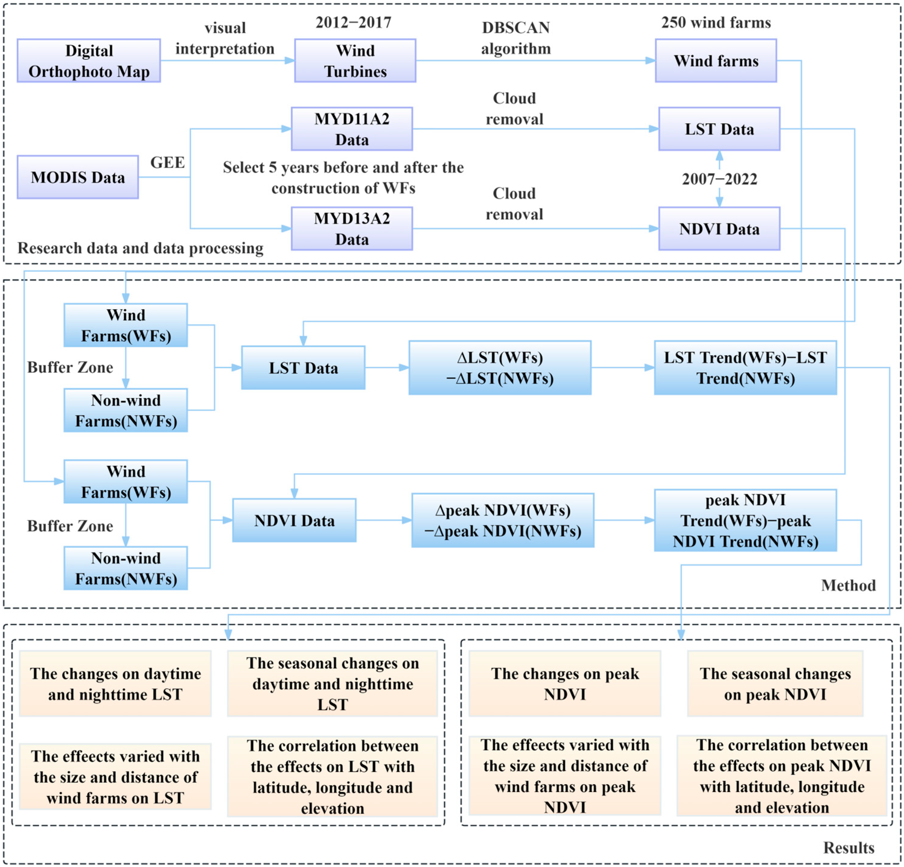
This study investigated the effects of 250 WFs constructed across China between 2012 and 2017 on LST and vegetation. We used data from Ziyuan-3 satellite to determine the spatial extent and construction timeline of WFs. Additionally, the LST and NDVI products were obtained from the Google Earth Engine (GEE) platform for assessing the impacts. By comparing LST and peak NDVI trends before and after five years of construction inside and outside the WFs, we examined the influence of 250 WFs in China on LST and vegetation. Finally, we employed the t-test to test whether the environmental effects were significant. Figure 1 illustrates the flowchart outlining the methodology employed to examine the effects of WFs on LST and vegetation.
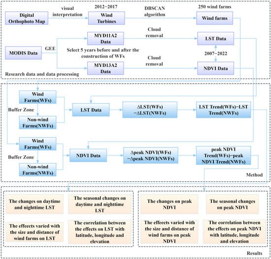
Figure 1.
The flowchart of the effects of WFs on LST and vegetation.
2.1. Data
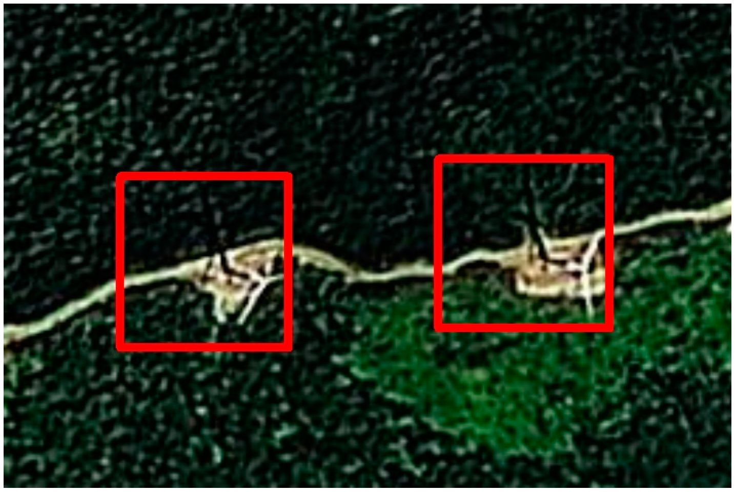
We employed Ziyuan-3 satellite data spanning the years 2012 to 2017 as base maps for visually interpreting wind turbines and determining their construction years. The annual Ziyuan-3 Digital Orthophoto Maps (DOM) used in this study had a resolution of 2.1 m. Wind turbines were identified by visual interpretation. On Ziyuan-3 satellite images, the white rotor blades and towers of wind turbines, along with their corresponding shadows, can be observed (Figure 2). The coordinates of a wind turbine were determined by the position of the bottom of its tower on images. To establish the construction year for each turbine, we followed this criterion: if a turbine did not appear in the image of year n but was visible in the image of year n + 1, the construction year of the turbine was considered to be n + 1.

Figure 2.
Wind turbines on Ziyuan-3 satellite images. Wind turbines are enclosed in red boxes.
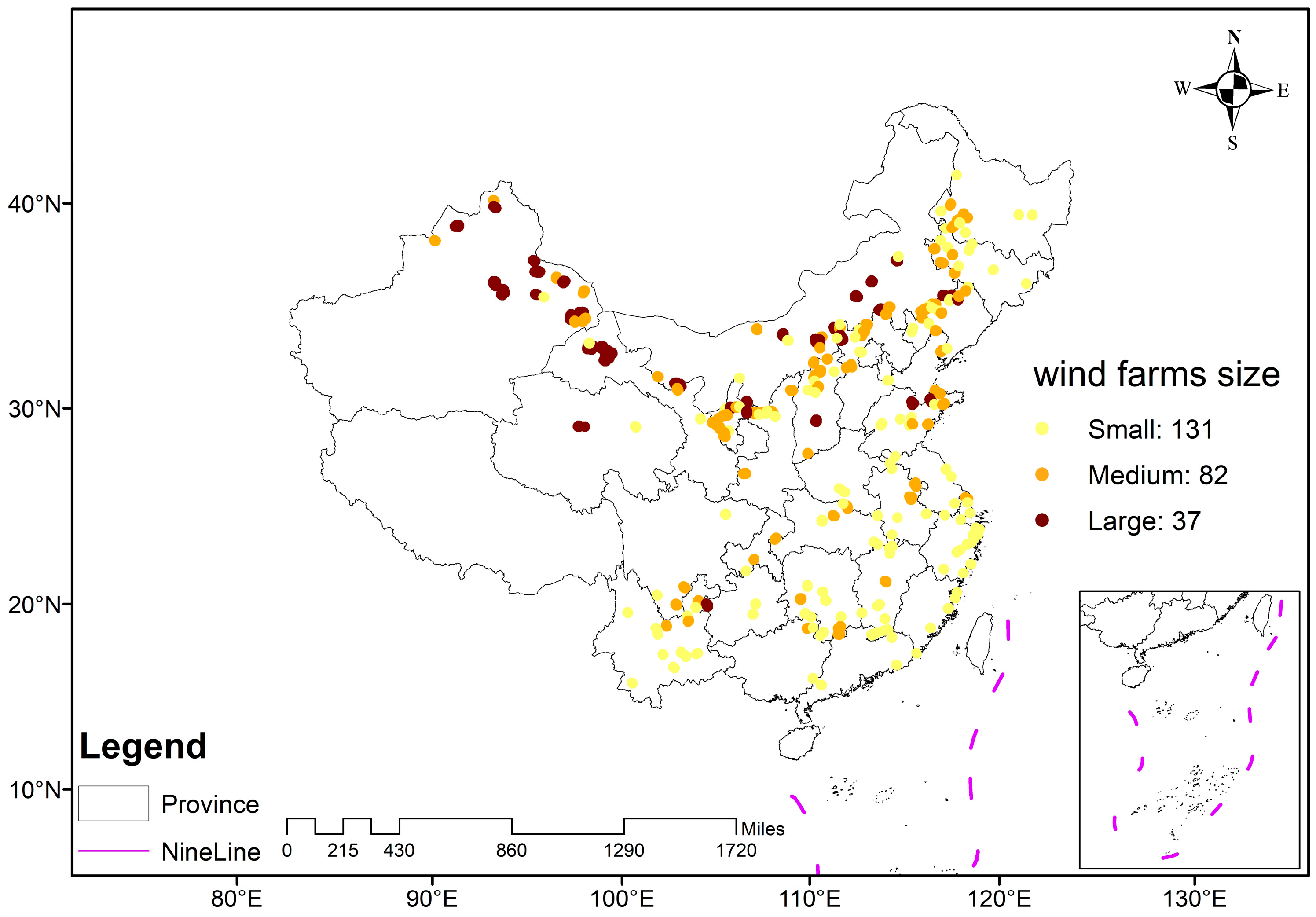
A total of 48,339 wind turbines and 250 WFs were selected. These WFs are generally evenly distributed across all provinces except Beijing, Hainan, and Tibet (Figure 3). The wind farms that also incorporate photovoltaic panels were excluded. The wind turbines located away from areas with human activities were preferred. According to the three principles, we identified 48,339 wind turbines. We employed the Density-Based Spatial Clustering of Applications with Noise (DBSCAN) algorithm to group individual wind turbines into WFs clusters [38]. The DBSCAN is a density-based clustering algorithm that relies on two key parameters: the search radius and the minimum number of points required to form a cluster. Specifically, the search radius was set to 0.1 km, and the minimum number of points was set to 5. As a result, the initial 48,339 wind turbines were clustered into 250 WFs. The 250 WFs were further categorized based on the number of turbines they contained: the small WFs (less than 100 turbines), the medium WFs (101 to 300 turbines), and the large WFs (more than 300 turbines).
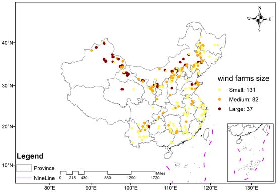
Figure 3.
Spatial distribution of the 250 WFs across China.
We employed MODIS remote sensing data to quantitatively assess the environmental impacts of WFs (Table 1). Specifically, we utilized the MODIS Aqua LST data product (MYD11A2) to evaluate the influence of WFs on LST. This data product had a spatial resolution of 1 km and a temporal resolution of 8 days. Additionally, we used the MODIS Aqua NDVI data product (MYD13A2) with a spatial resolution of 1 km and a temporal resolution of 16 days to study the impacts of WFs on vegetation. The LST and NDVI data products were obtained from the GEE platform, covering the period from 2007 (five years before the construction of WFs) to 2022 (five years after the construction of WFs).

Table 1.
Utilized products of Moderate Resolution Imaging Spectroradiometer (MODIS).
2.2. Evaluating the Effects of Wind Farms
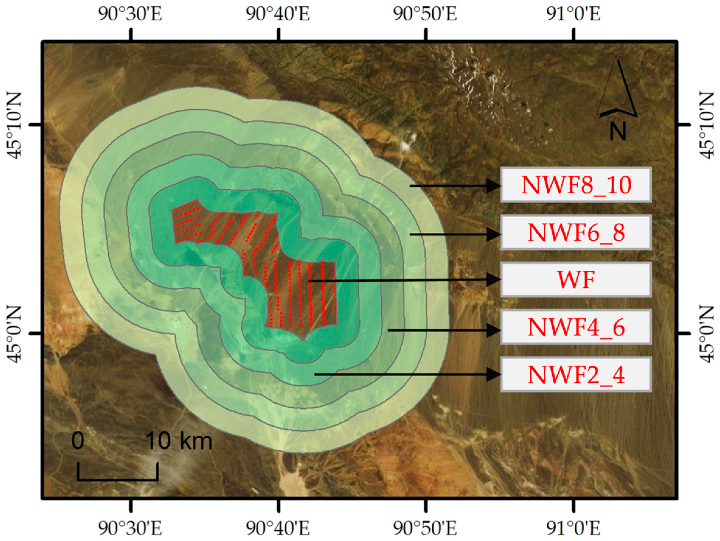
We assessed the environmental effects of 250 WFs in China by analyzing the changing trends in LST and peak NDVI within the WFs areas and adjacent non-wind farm (NWFs) areas [19,39]. The NWFs areas were delineated using buffer zones at varying distances from the WFs: NWF2_4 (within 2–4 km), NWF4_6 (4–6 km), NWF6_8 (6–8 km), and NWF8_10 (8–10 km) from the boundaries of WFs. Notably, we excluded the zone within 0–2 km [39] due to its direct susceptibility to the impacts of WFs owing to its proximity. Figure 4 illustrates the delineation of WF and NWF areas.

Figure 4.
A wind farm sample in China. The red points indicate individual wind turbines in WF areas. The light green zones indicate the NWF areas.
We assumed that the WFs and natural factors jointly influenced LST within the WFs areas. In contrast, the LST in NWFs regions was solely affected by natural factors. Assuming that these natural factors exerted equal influence on both WFs and NWFs, the differential changes in LST between WFs and NWFs areas could be attributed to the WFs.
∆LST was used to measure the effect of WFs on LST. ∆LST was calculated by subtracting the ∆LST of NWFs from the ∆LST of WF region, and were the changes of LST in WFs and NWFs in a specific time window, respectively. The specific calculation formula (Equation (1)) was represented by [19]:
where and represented the linear trends of LST in WFs and NWFs areas, respectively. and were the slope of the linear trend lines.
Similarly, we used the difference in peak NDVI (the 95th percentile of annual NDVI) between the areas of WFs and NWFs to quantify the effects of WFs on vegetation, and the following Equation (2) [19] was the calculation formula of ∆peak NDVI:
where ∆peak and ∆peak were the changes of peak NDVI in WFs and NWFs in a specific time window, respectively. ∆peak NDVI was the value of the subtraction of the two, and the peak and peak were the slope of the linear trend lines.
2.3. The Significant t-Test
In this study, we employed the t-test to assess the significant effects of WFs on vegetation and LST. The t-test assessed whether the changes in surface temperature and vegetation in WFs areas significantly differed from those in NWFs areas. The t-test yielded two key results: the t-statistic and the p-value. We considered significant impacts of WFs on vegetation or LST if the p-value was less than 0.05 at the 95% confidence level or below 0.1 at the 90% confidence level.
3. Results
3.1. The Effects of Wind Farms on Surface Temperature
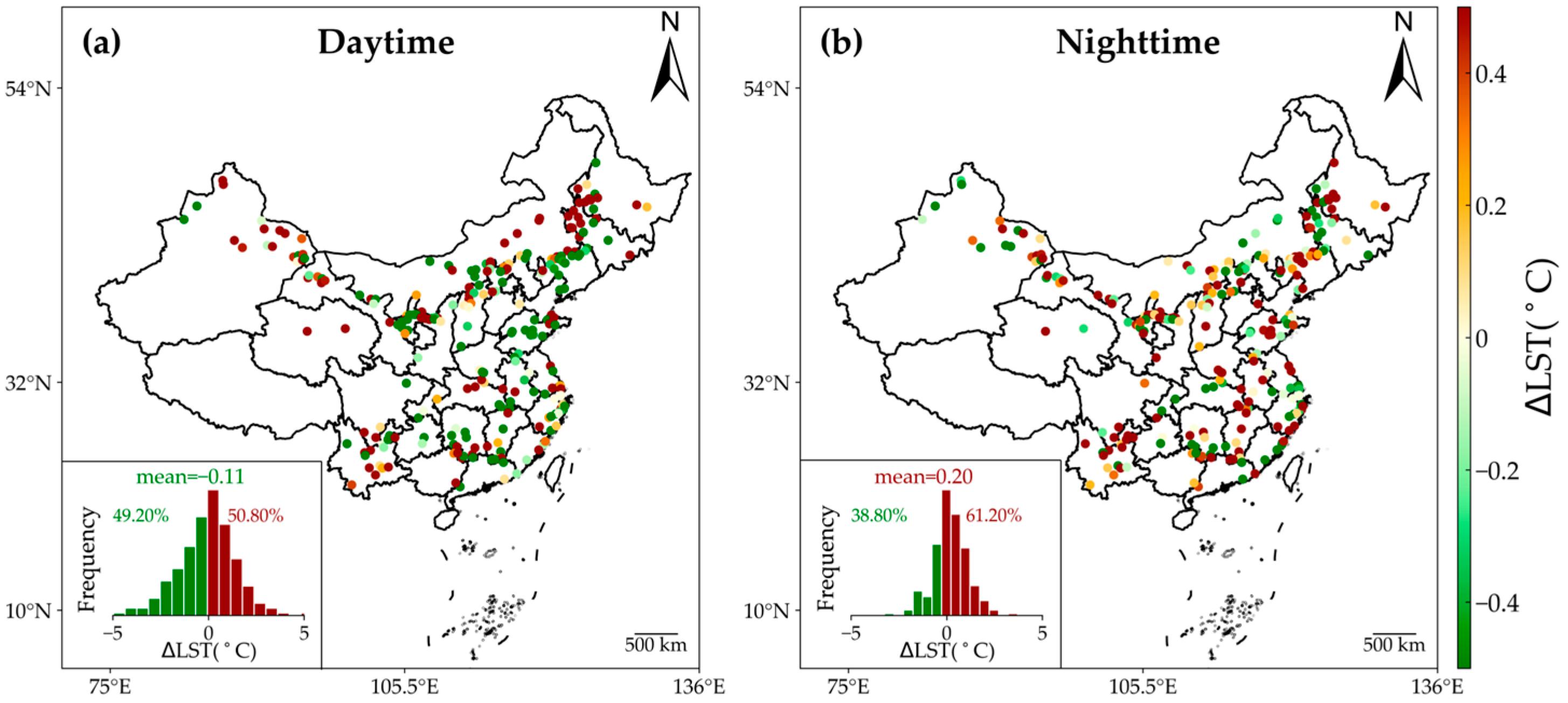
Figure 5 illustrates the impacts of 250 WFs in China on annual mean LST during both daytime and nighttime. During daytime, no discernible pattern emerged among the WFs, contributing to both cooling (∆LST < 0) and warming (∆LST > 0) effects. Specifically, 50.80% of WFs samples exhibited warming effects, while 49.20% showed cooling effects. The average value of daytime ∆LST across the 250 WFs was −0.11 ± 1.60 °C (mean ± 1 STD), but it failed to achieve statistical significance in the t-test (p > 0.05) (Figure 5a). In contrast, during nighttime, a notable warming effect was observed for 250 WFs (Figure 5b). The proportion of warming samples at night exceeded that of cooling samples by 22.40%. The averaged ∆LST at night across the 250 WFs was 0.20 ± 0.99 °C, and it passed the t-test (p < 0.05). These results highlighted the differential impacts of WFs on LST between daytime and nighttime, with significant warming effects occurring during nighttime but negligible effects during daytime.
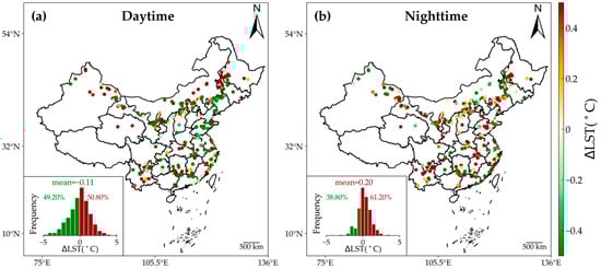
Figure 5.
Effects of WFs on annual mean daytime (a) and nighttime (b) LST. The insets display histograms of ∆LST for 250 WFs across China, including mean values and the proportions of positive (dark red) and negative (green) values.
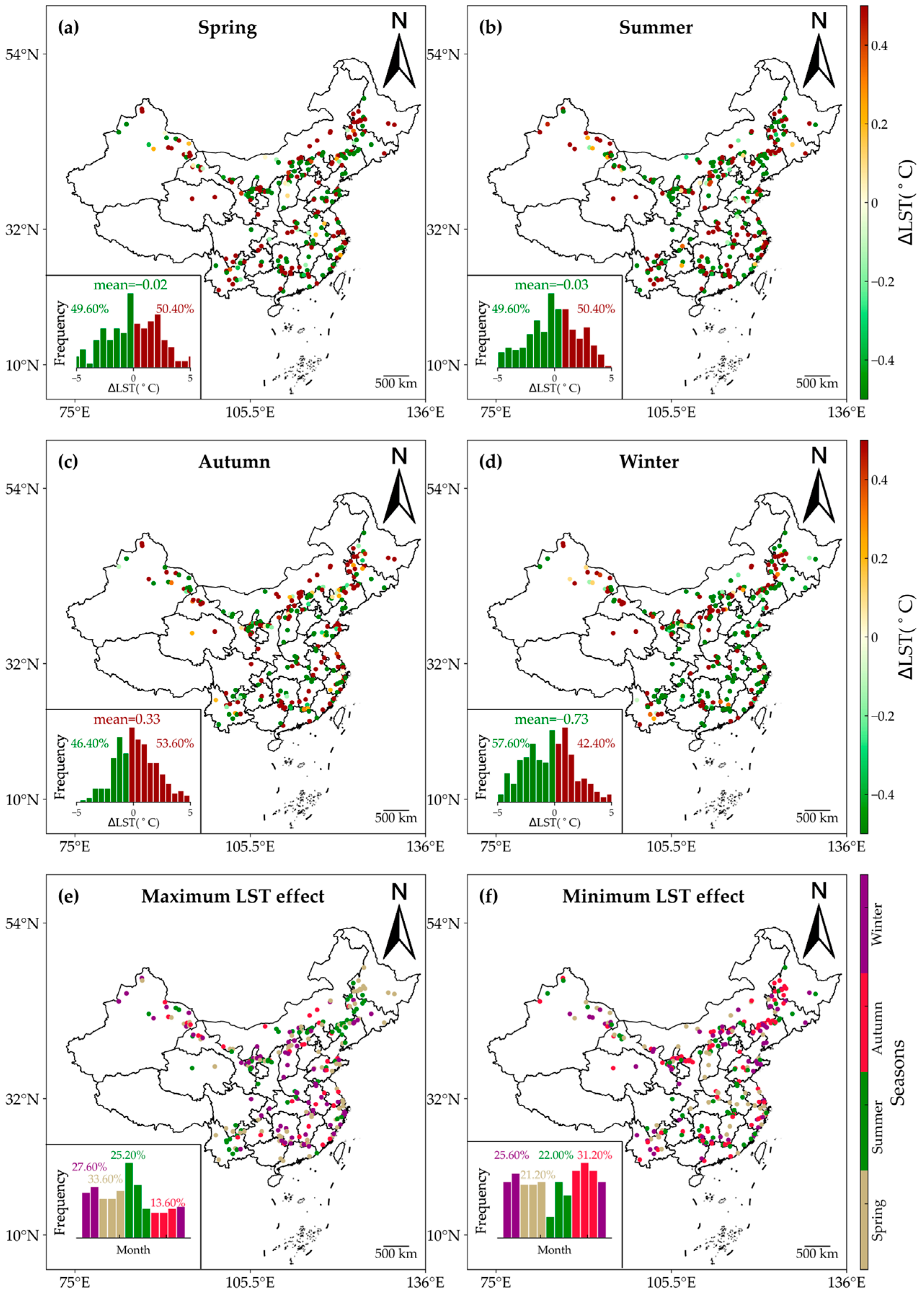
This research examined the seasonal effects of WFs on LST by evaluating ∆LST across various seasons: spring (March to May), summer (June to August), winter (December to February), and autumn (September to November). Figure 6 illustrates the seasonal effects of WFs on daytime LST. During daytime, the influence of WFs on LST was weak in both spring and summer. The averaged ∆LST across all samples did not achieve statistical significance (p > 0.05). Additionally, the proportions of warming and cooling samples were nearly equal in spring (50.40% warming vs. 49.60% cooling). Regarding the magnitude of ∆LST, the annual average ∆LST was −0.02 °C in spring and −0.03 °C in summer. However, pronounced daytime warming occurred during autumn, while cooling effects prevailed in winter. In winter, all samples exhibited a significantly higher cooling percentage than warming, whereas in autumn, the opposite was true, with a notably higher warming percentage than cooling. Regarding the magnitude of ∆LST, significant daytime cooling was observed in winter, and the average value of ∆LST was −0.73 ± 1.35 °C (p < 0.01), while daytime warming occurred in autumn, and the average value of ∆LST was 0.33 ± 0.73 °C (p < 0.05). The varying minimal and maximal impacts on LST across all seasons further supported this phenomenon (Figure 6e,f). In autumn, the percentage of minimum daytime impacts reached 31.20%, surpassing spring and summer by 10% and 9.20%, respectively. In winter, the percentage of maximum daytime impacts was 27.60%, exceeding summer and autumn by 2.40% and 14%, respectively. The significant seasonal variations in the impacts of WFs during daytime led to no overall warming or cooling effects during daytime.
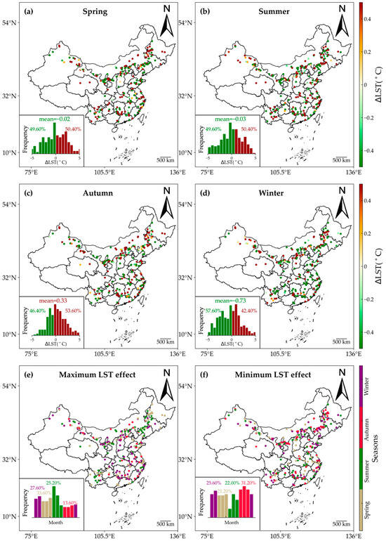
Figure 6.
Seasonal variations in the daytime effects of WFs on LST. The effects of WFs on daytime LST are shown for spring (a), summer (b), winter (d), and autumn (c). (e,f) show months with maximum and minimum ∆LST. The insets provide histograms of the months with the highest and lowest ∆LST values.
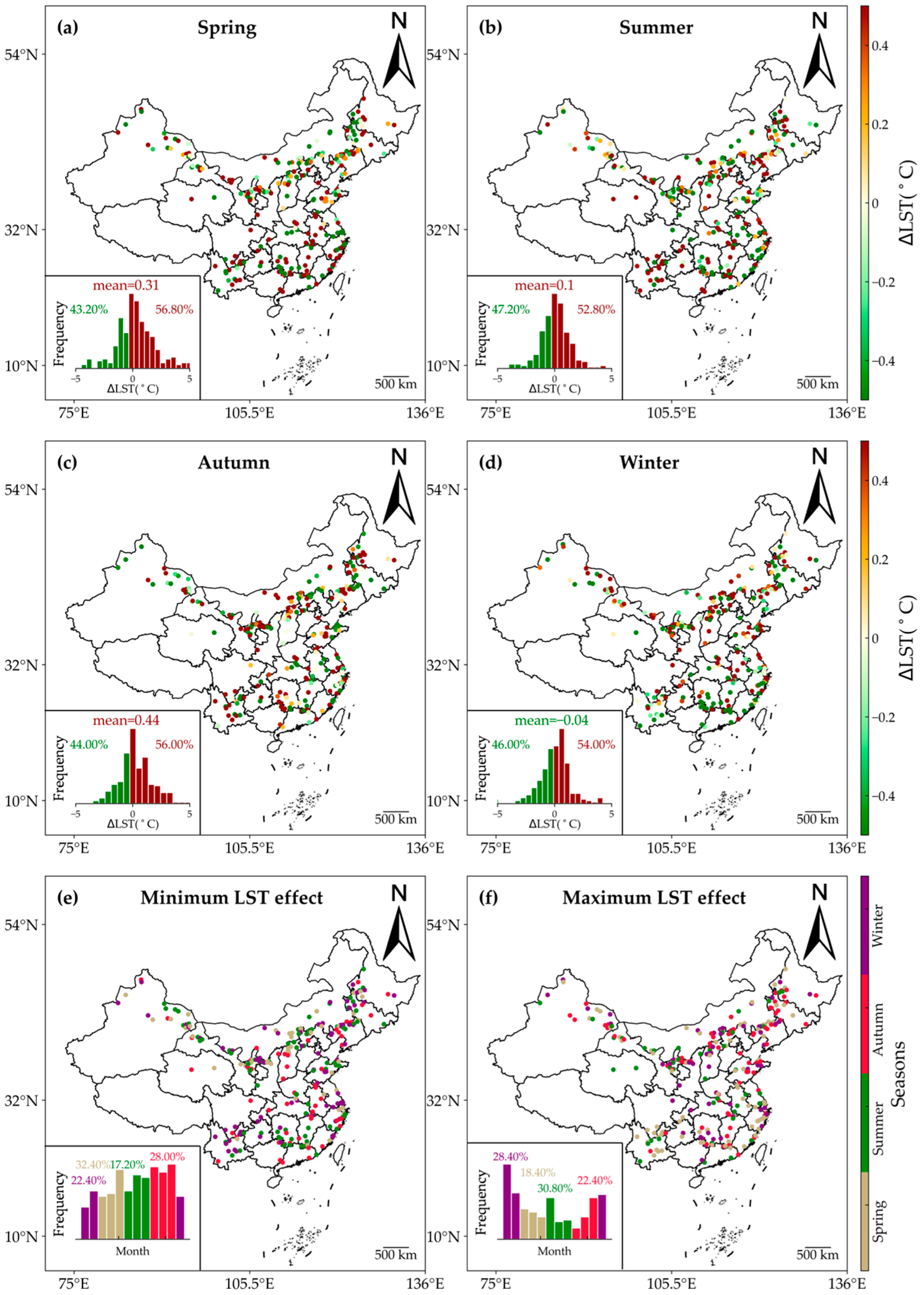
Figure 7 illustrates the seasonal impacts of WFs on nighttime LST. Throughout all seasons, the warming effects predominated during nighttime, with the proportion of warming samples varying from 52.80% in summer to 56.80% in spring. Concerning the magnitude of ∆LST, the annual average value of nighttime ∆LST across the 250 WFs was 0.31 °C in spring, 0.10 °C in summer, 0.44 °C in autumn, and −0.04 °C in winter, indicating a slight cooling effect in winter. While the proportions of warming samples exceeded those of cooling samples in all seasons, not all of these warming effects reached statistical significance. The t-test results revealed that the annual average values of nighttime ∆LST in spring and autumn were statistically significant (p < 0.01), whereas those in summer and winter were not (p > 0.1). Furthermore, the fluctuating maximal and minimal impacts on nighttime LST were observed in spring and autumn. In these seasons, the nighttime minimal impacts accounted for the largest proportions, exceeding 25%. Conversely, summer and winter saw substantial contributions from nighttime maximal impacts. Overall, the consistent warming trends prevailed across all seasons, resulting in significant nighttime warming.
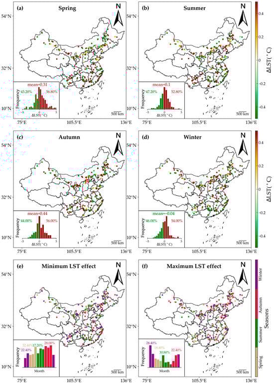
Figure 7.
Seasonal variations in the nighttime effects of WFs on LST. The impacts of WFs on nighttime LST are shown for spring (a), summer (b), winter (d), and autumn (c). (e,f) show the minimum and maximum months of ∆LST. The insets show histograms of months with the lowest and highest ∆LST values.
3.2. The Effects of Wind Farms on Vegetation
The findings from Figure 8 revealed a widespread decline in peak NDVI, accounting for 75.20% of all WF samples. Additionally, the average ∆peak NDVI across the 250 WFs was −0.41, a statistically significant result (p < 0.01). However, approximately 24.80% of WF samples exhibited higher peak NDVI values. Notably, the effects of WFs exhibited distinct spatial distribution patterns. For instance, northwest China experienced an increasing trend in peak NDVI, while the eastern coastal region showed a general decrease. Previous studies have documented significant reductions in peak NDVI in northern China [31] and the United States [19], attributed to the operation of WFs.
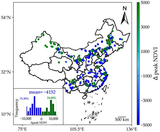
Figure 8.
Impacts of WFs on peak NDVI. The values shown are scaled by a factor of 10,000.
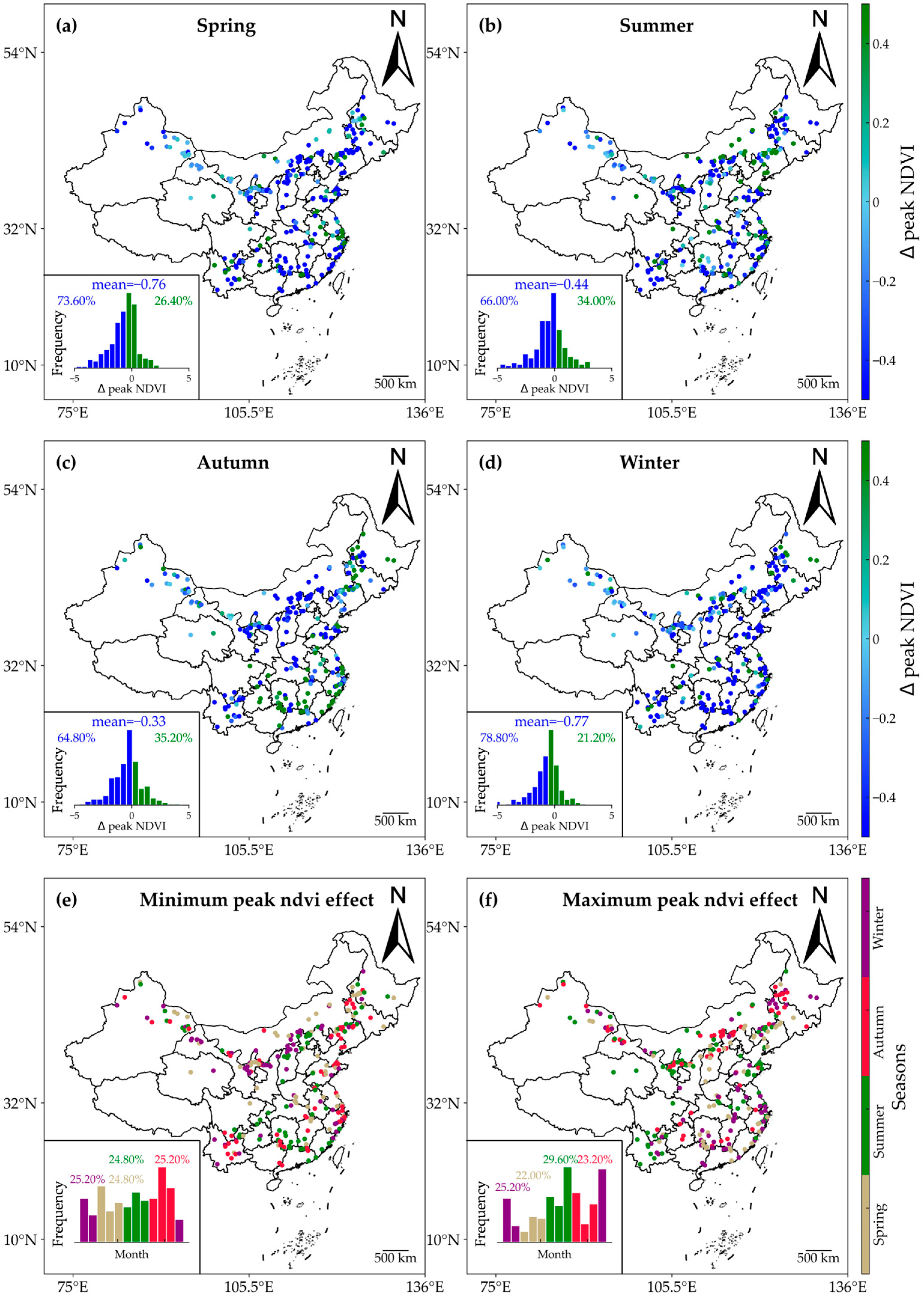
Figure 9 illustrates the seasonal impacts of WFs on peak NDVI. Across all seasons, the peak NDVI exhibited a consistent decreasing trend, with more than 50% of WF samples showing reductions. The averaged values of ∆peak NDVI ranged from −0.77 in winter to −0.33 in autumn, all of which passed the significance test (p < 0.05). Notably, the maximum and minimum impacts on peak NDVI confirmed that the WFs had the most significant effects during winter and the least impact during autumn. Specifically, the maximum peak NDVI reduction occurred in winter at 25.20%, while the minimum reduction occurred in autumn at the same percentage. Overall, the negative impacts of WFs on peak NDVI prevailed throughout all seasons, exhibiting varying magnitudes.
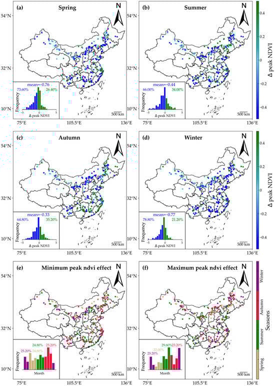
Figure 9.
Seasonal variations in the effects of WFs on peak NDVI. The impacts on peak NDVI are shown for spring (a), summer (b), winter (d), and autumn (c). (e,f) show the minimum and maximum months of ∆peak NDVI. The insets show histograms of the months with the lowest and highest ∆peak NDVI values.
3.3. The Impacts of Wind Farms Depend on Their Size and Distance
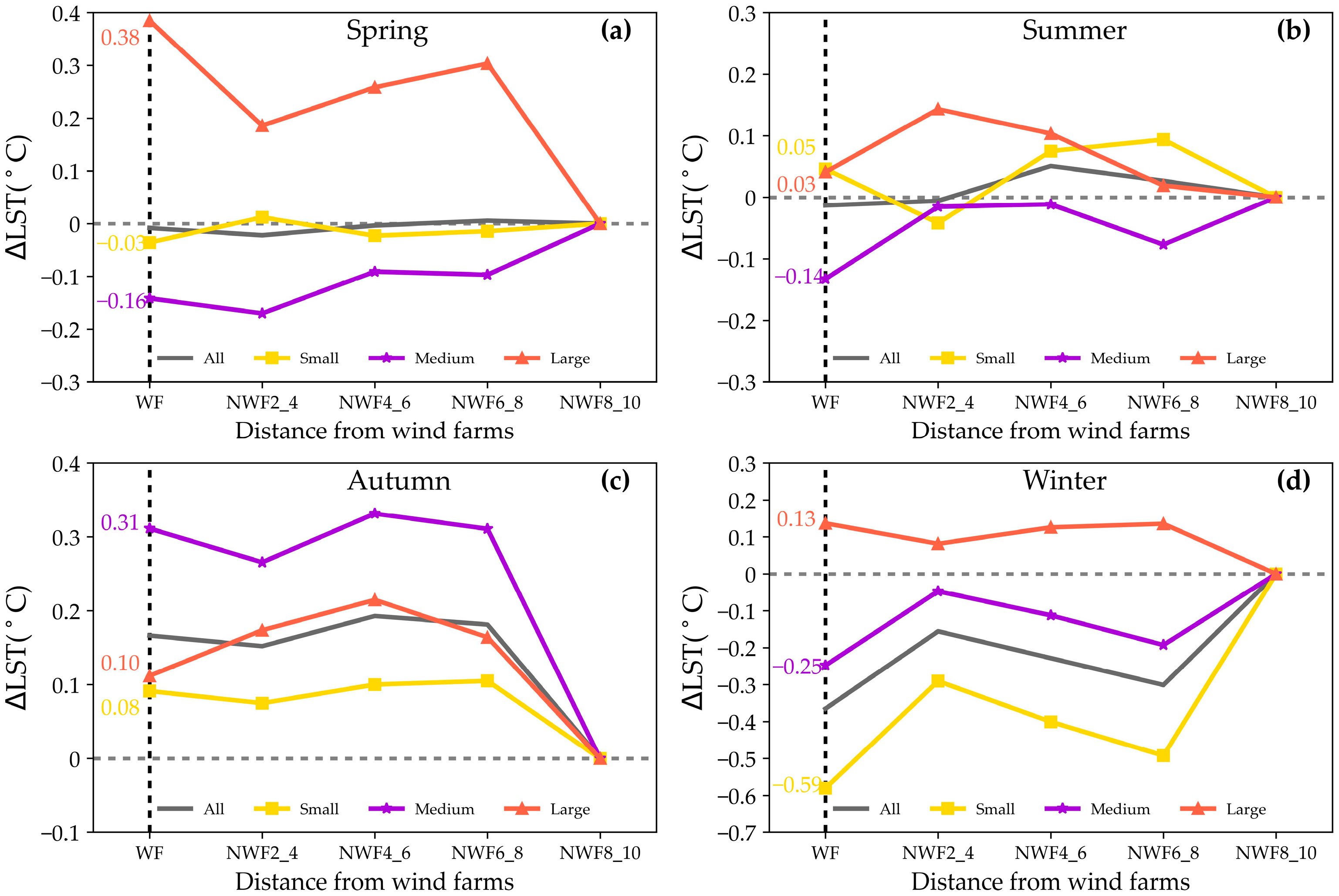
The influence of WFs sizes on LST exhibited significant variability. To explore these relationships, this study analyzed seasonal daytime LST variations across the 250 WFs of varying sizes (Figure 10). Notably, the large WFs demonstrated a warming effect on LST during spring and winter. Specifically, in spring, the impact was notably higher, resulting in a ∆LST of 0.38 °C (p < 0.05), compared to 0.13 °C (p > 0.05) in winter. In contrast, the small WFs exhibited distinct effects relative to the large WFs. During spring, summer, and autumn, the ∆LST ranged from −0.03 °C to 0.08 °C, significantly weaker than the impact observed in large WFs. However, during winter, the small WFs induced substantial cooling, with an average daytime ∆LST of −0.59 °C (p < 0.05).
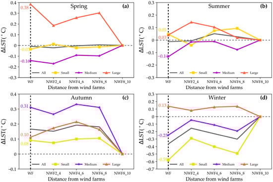
Figure 10.
Effects of WFs size and location on daytime LST. The effects of WFs on daytime LST are shown in spring (a), summer (b), autumn (c), and winter (d). Solid lines in different colors represent large (orange), medium (purple), and small (yellow) WFs. The WFs areas are indicated by vertical dashed lines.
The impacts of WFs on daytime LST were significantly influenced by proximity. Specifically, during spring, autumn, and winter, the effects of small, medium, and large WFs on LST exhibited a consistent pattern: initial decrease, subsequent increase, and final decrease with distance. For instance, in spring, the ∆LST decreased from 0.38 °C within the WFs areas to 0.18 °C at 2–4 km, and then increased to 0.27 °C at 6–8 km before declining to 0 °C at 8–10 km. The impacts of large WFs on LST during summer followed a pattern of initially increasing and then decreasing with distance, with the ∆LST rising from 0.03 °C within the WFs areas to 0.12 °C at 2–4 km before declining to 0 °C at 8–10 km. Notably, the influence of small and medium WFs on LST exhibited a trend of decreasing, then increasing, and subsequently decreasing with distance. For instance, the ∆LST of small WFs decreased from 0.05 °C within the WFs areas to −0.03 °C at 2–4 km, increased to 0.08 °C at 6–8 km, and then decreased to 0 °C at 8–10 km.
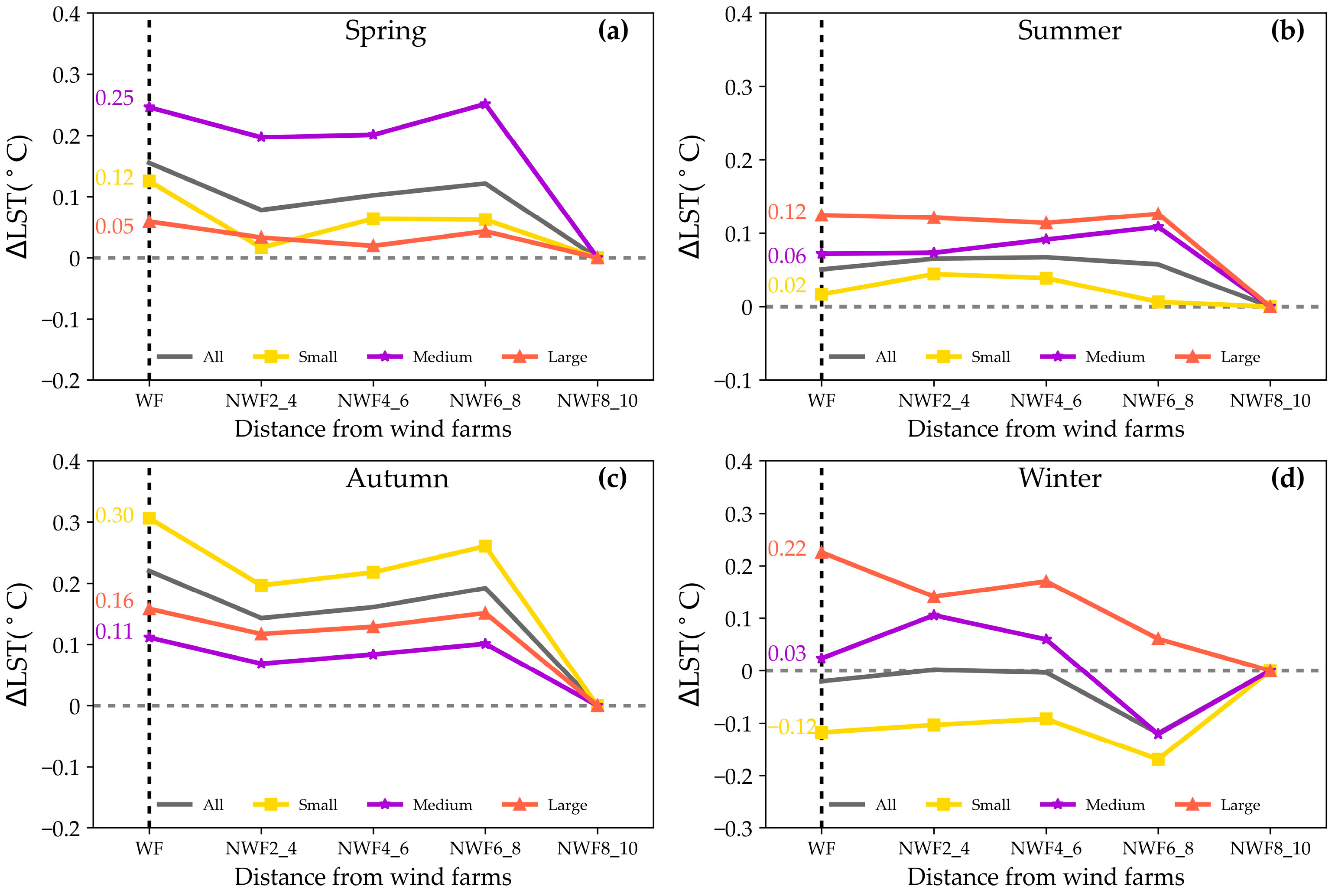
Figure 11 illustrates the impacts of WFs sizes on nighttime LST. During spring, summer, and autumn, the WFs of all sizes exerted a warming influence within their vicinity. Notably, this warming effect was particularly pronounced in autumn, with ∆LST reaching 0.30 °C (p < 0.05) in the small WFs. In summer, the WFs had a minor effect on LST, with the mean ∆LST values varying from 0.02 °C to 0.12 °C during nighttime. Conversely, in winter, the large and medium-sized WFs contributed to warming effects (0.22 °C and 0.03 °C) on LST, while the small-sized WFs induced cooling effects (−0.12 °C), resulting in a weaker overall effect during winter.
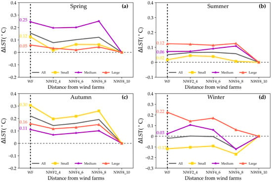
Figure 11.
Effects of WFs size and location on nighttime LST. The effects of WFs on nighttime LST are shown in spring (a), summer (b), autumn (c), and winter (d). Solid lines in different colors represent large (orange), medium (purple), and small (yellow) WFs. The wind farm areas are highlighted by vertical dashed lines.
The impacts of WFs on nighttime LST were also correlated with distance. During spring and autumn, the effects of small, medium, and large WFs exhibited a consistent pattern: initial decrease, subsequent increase, and final decrease with distance. For instance, the ∆LST of small WFs decreased from 0.30 °C within the WFs areas to 0.20 °C at a distance of 2–4 km, and then increased to 0.27 °C at 6–8 km before diminishing to 0 °C at 8–10 km. In contrast, the impacts of WFs on LST during summer showed minimal variation with distance. For example, the ∆LST of large WFs ranged from 0.12 °C within the WFs areas to 0.10 °C at 6–8 km. Furthermore, the influence of large WFs on LST during winter followed a pattern of initial decrease, subsequent increase, and final decrease. Specifically, the ∆LST of large WFs decreased from 0.22 °C within the WFs areas to 0.15 °C at 2–4 km, and then increased to 0.18 °C at 4–6 km before diminishing to 0 at 8–10 km. Conversely, the small and medium-sized WFs exhibited a trend of initial increase, subsequent decrease, and final increase. For example, the ∆LST of medium WFs increased from 0.03 °C within the WFs areas to 0.10 °C at 2–4 km, then decreased to −0.12 °C at 6–8 km, and finally diminished to 0 at 8–10 km.
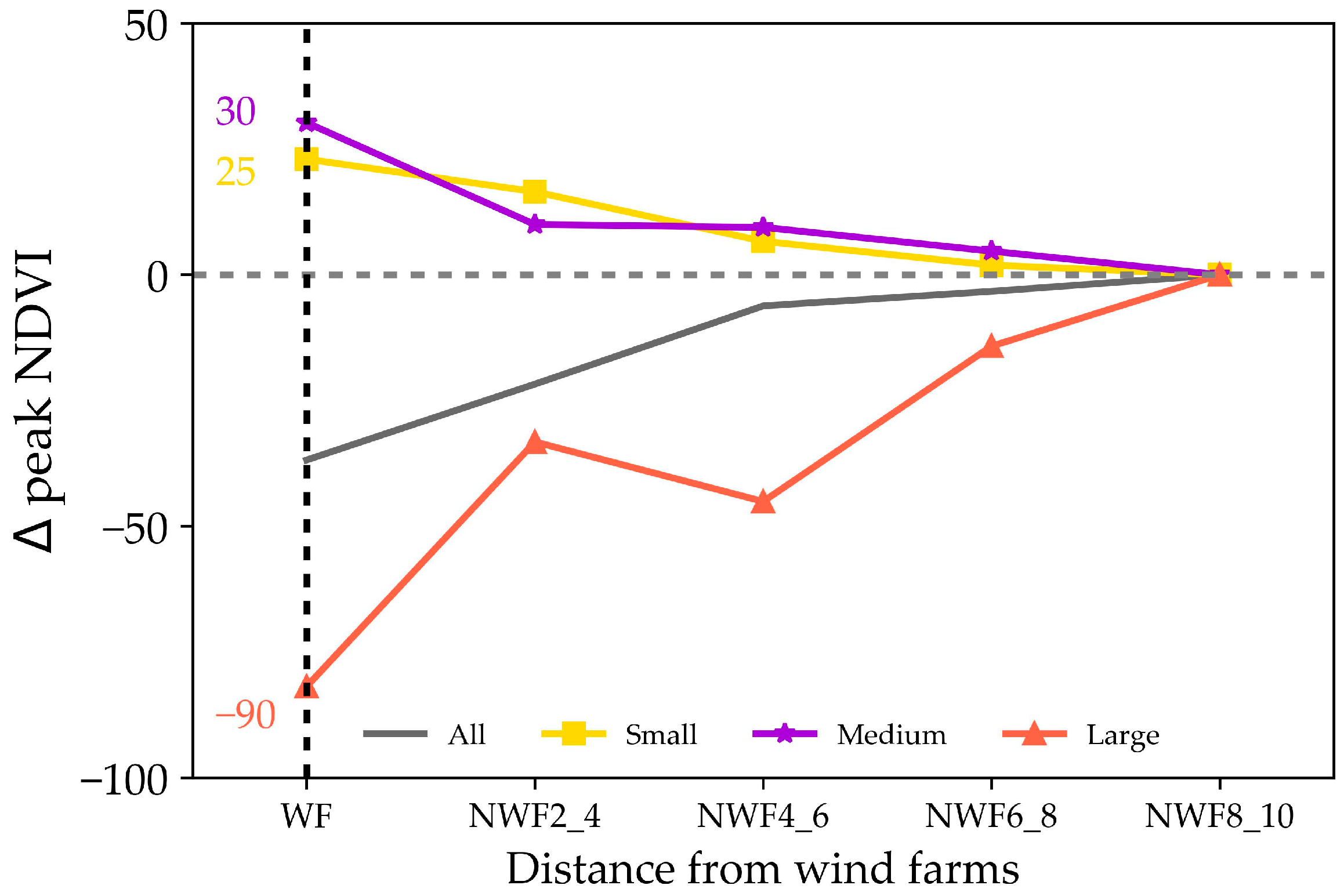
Figure 12 illustrates the impacts of WFs on vegetation, considering both WFs sizes and distances. Within the WFs areas, the large WFs had a negative impact on vegetation, whereas the small and medium-sized WFs exhibited a positive influence. Analyzing the ∆peak NDVI values revealed that the most significant impacts on vegetation occurred with the large WFs, resulting in a peak NDVI reduction of 0.009 (p < 0.05). In contrast, the small and medium-sized WFs had lesser impacts on vegetation, with increases of 0.0025 and 0.003, respectively.

Figure 12.
Relationship between the peak NDVI and the size and distance of WFs. The values shown are scaled by a factor of 10,000.
The influence of WFs on vegetation decreased with distance. However, unlike the effects on LST, which weakened over greater distances, the impacts on vegetation rapidly approached 0 within 2–4 km from the WFs. This phenomenon suggested that the WFs predominantly affect vegetation at the local scale.
3.4. The Correlations Between the Impacts of Wind Farms with Latitude, Longitude and Elevation
In this research, we examined the spatial relationships between variations in daytime and nighttime LST and peak NDVI in relation to latitude, longitude, and elevation (Table 2). Notably, no significant correlations emerged between daytime and nighttime LST variations with latitude, longitude, or elevation. However, we observed a weak negative correlation between peak NDVI variation and elevation (correlation coefficient: −0.221, p < 0.001). However, these findings diverged from those related to photovoltaic power plants, which exhibited sensitivity to latitude, longitude, and elevation [40].
Table 2.
Correlation coefficients and p-values for changes in daytime and nighttime LST and peak NDVI in relation to longitude, latitude, and elevation.
4. Discussion
4.1. The Reasons for Changes in LST
The notable warming effects of 250 WFs in China during nighttime were attributed to air disturbance. Although the mechanisms underlying LST changes were not consistent, scholars generally attributed them to variations in stability of Atmospheric Boundary Layer [37,41,42,43,44,45]. Wind turbines acted as towering “air churns”, with their blades continuously stirring the air both above and below, enhancing vertical airflow and influencing LST. Specifically, during stable atmospheric conditions at night, the upper layer of air tended to be warmer, while the lower layer was cooler. The blade action brought down warmer air from the upper layer, resulting in increased surface temperatures [15,46,47]. Notably, our study, along with that of Qin et al. [19], observed smaller nighttime LST increases compared to the findings by Xia et al. [32], which reported nighttime warming of up to 1.35 °C.
The slight daytime increase in temperature, which did not achieve statistical significance in the t-test, resulted from a combination of air disturbance caused by WFs and atmospheric instability. During daylight hours, the upper air layer tended to be cooler than the lower air layer. The rotation of wind turbine blades blended the cooler air from above with the warmer air below, leading to a decrease in surface temperatures. This observation aligned with previous findings by Zhou et al. [47] and Xu et al. [30]. The insignificant daytime LST effects from WFs primarily stemmed from the instability of atmospheric boundary layer during daytime and the absence of pronounced air stratification.
This study revealed distinct seasonal effects on LST during both daytime and nighttime. Notably, weak seasonality was observed at night, aligning with the results of Qin et al. [19]. However, while this study detected a slight decrease in surface temperatures during winter, Qin et al. [19] reported a similar decrease in spring. In contrast, strong seasonality was evident during daytime. These seasonal variations in surface temperature primarily resulted from differential daytime heating and atmospheric stability. Unlike other seasons, winter exhibited a significant cooling effect due to a more stable atmosphere, which brought colder upper air to the surface, resulting in lower surface temperatures.
4.2. The Reasons for Changes in Vegetation
The WFs significantly impacted vegetation, with research consistently indicating negative effects, particularly for large-scale WFs. This finding aligned with the results by Ma et al. [48] and Tang et al. [31]. Firstly, the construction of new roads for transportation of WFs led to vegetation destruction. Additionally, the installation and operation of WFs required land, including the establishment of substations and booster stations, further encroaching land. Secondly, the establishment of WFs permanently altered conditions for vegetation growth. For example, the increased nighttime temperatures enhanced evapotranspiration and reduced soil moisture, hindering vegetation growth.
Our study revealed that the WFs had a positive impact on vegetation. This effect was primarily attributed to improved growing conditions. Specifically, the vegetation surrounding WFs benefited from reduced evapotranspiration due to shading, particularly in water-scarce areas. Additionally, Ma et al. [16] explained that changes in vegetation, wind speed, and direction also positively contributed to vegetation growth.
The analysis revealed that the WFs had unconventional impacts on vegetation growth, with results indicating both positive and negative effects. These findings aligned with the research by Qin et al. [19]. The inconsistency arose from the complex relationship between WFs and vegetation, which was challenging to analyze accurately due to variations in size, scale, and region of WFs.
4.3. Limitations
This study encountered limitations when assessing the impacts of WFs. Firstly, the MODIS satellite data introduced uncertainties. To verify the validity of the results, we examined the effects of WFs on LST during daytime and nighttime, along with the peak NDVI, using data from MODIS Aqua and Terra satellites. Our study findings, derived from MODIS Terra data, revealed that nighttime warming occurred in 60.40% of cases. In comparison, daytime warming was observed in 51.60% of cases, consistent with the conclusions previously drawn in this study (Table 3).
Table 3.
Impacts of WFs on daytime and nighttime annual mean LST and peak NDVI using MODIS Aqua and Terra data.
The choice of the time window was subjective. To address this, we quantified LST and peak NDVI for both 6-year and 7-year periods before and after the construction of WFs. These results bolstered the reliability of this study (Table 4). For instance, the percentage of nighttime surface temperature warming for each of the six years before and after the construction of WFs was 59.42%.
Table 4.
Sensitivity of nighttime ∆LST at night and ∆peak NDVI to various time periods.
The influence of human activities, aside from wind farm construction, on WFs required further mitigation. Numerous human activities impact the surface temperature and vegetation of WFs and their surrounding areas. In conducting research on WFs, we excluded those with photovoltaic panels and prioritized those located in remote areas, such as deserts and ridges, to minimize interference from other human activities. With the availability of time series data of high-resolution images, land cover, and land surface parameters, it is possible to detect human activities and abnormal environmental trends in and around WFs and conduct more precise exclusions of WFs. However, the factors affecting the environment of wind farms are diverse and not yet fully understood, making it challenging to eliminate all influences.
5. Conclusions
This study analyzed the long-term environmental effects of 250 wind farms constructed in China between 2012 and 2017 on land surface temperature and vegetation using remote sensing data. The study assessed changes in these factors within and outside of wind farm areas over a five-year period before and after construction, considering both daytime and nighttime temperature as well as peak vegetation index. The study also examined the influence of wind farm size and proximity on these factors, and evaluated the correlations between environmental impacts and geographical factors. The findings of this study are as follows:
- (1)
- Our results demonstrated that wind farms have contrasting effects on LST during day and night, notably rising by 0.20 °C in nighttime LST and falling by 0.11 °C in daytime LST. These temperature changes exhibited strong seasonal variability during the daytime, yet remained relatively consistent at night.
- (2)
- A total of 75.20% of the wind farms negatively impacted vegetation, with no discernible seasonality in this effect.
- (3)
- Larger wind farms, as well as those in closer proximity to sampling areas, were found to exert a stronger influence on both LST and vegetation dynamics.
- (4)
- Our analysis revealed that geographic factors, such as latitude, longitude, and elevation, showed weak correlations with the observed changes in LST and vegetation.
The study filled a significant gap in the literature with a robust, large-scale, long-term assessment of environmental impacts of WFs using remote sensing. Our findings revealed nighttime warming and negative effects on vegetation, as well as the considerable heterogeneity of the environmental impacts of WFs and the variations from existing studies. The utilized approach is a quantitative method entirely based on remote sensing, which can be applied to diverse regions globally. This study provides a scientific basis for national and regional policy-making and planning in the field of renewable energy. Furthermore, it offers important insights for the placement and design of local WFs.
Future research should explore the broader ecological consequences of wind farm development and consider additional factors such as biodiversity loss, water resources, and social impacts to fully capture the scope of wind energy’s environmental footprint.
Author Contributions
Conceptualization, X.H., C.L. and J.W.; methodology, X.H.; software, X.H.; validation, X.H. and J.W.; formal analysis, X.H.; investigation, C.L. and J.W.; resources, C.L. and J.W.; data curation, X.H.; writing—original draft preparation, X.H.; writing—review and editing, X.H., C.L. and J.W.; visualization, X.H.; supervision, C.L. and J.W.; project administration, C.L. and J.W.; funding acquisition, C.L. and J.W. All authors have read and agreed to the published version of the manuscript.
Funding
This work was supported by the National Key Research and Development Program of China (Grant No. 2022YFF1303405), and the Strategic Priority Research Program of the Chinese Academy of Sciences (Grant No. XDA23090402).
Data Availability Statement
The data presented in this study are available on request from the corresponding author. Due to legal restrictions, data can not to be shared publicly.
Acknowledgments
The authors would like to sincerely thank all those who made suggestions about the paper.
Conflicts of Interest
The authors declare no conflicts of interest.
References
- Chen, L.; Msigwa, G.; Yang, M.Y.; Osman, A.I.; Fawzy, S.; Rooney, D.W.; Yap, P.S. Strategies to achieve a carbon neutral society: A review. Environ. Chem. Lett. 2022, 20, 2277–2310. [Google Scholar] [CrossRef]
- Yang, J.B.; Liu, Q.Y.; Li, X.; Cui, X.D. Overview of Wind Power in China: Status and Future. Sustainability 2017, 9, 1454. [Google Scholar] [CrossRef]
- Jiang, J.; Yang, L.; Li, Z.; Gao, X. Progress in the Research on the Impact of Wind Farms on Climate and Environment. Adv. Earth Sci. 2019, 34, 1038–1049. [Google Scholar]
- Ai, Z.; He, F.; Chen, Z.H.; Zhong, S.X.; Shen, Y.B. Simulated Influence of Mountainous Wind Farms Operations on Local Climate. J. Trop. Meteorol. 2022, 28, 109–120. [Google Scholar] [CrossRef]
- Siedersleben, S.K.; Platis, A.; Lundquist, J.K.; Djath, B.; Lampert, A.; Bärfuss, K.; Cañadillas, B.; Schulz-Stellenfleth, J.; Bange, J.; Neumann, T.; et al. Turbulent kinetic energy over large offshore wind farms observed and simulated by the mesoscale model WRF (3.8.1). Geosci. Model Dev. 2020, 13, 249–268. [Google Scholar] [CrossRef]
- Akter, S.; Loo, J.K.; Hannan, M.A. Assessing the Impact of Climate Conditions on Harnessing Coastal (Offshore) Wind Energy. In Proceedings of the International Conference on Civil and Environmental Engineering (ICCEE), Kuala Lumpur, Malaysia, 2–5 October 2018. [Google Scholar]
- Harris, R.A.; Zhou, L.M.; Xia, G. Satellite Observations of Wind Farm Impacts on Nocturnal Land Surface Temperature in Iowa. Remote Sens. 2014, 6, 12234–12246. [Google Scholar] [CrossRef]
- Liu, N.J.; Zhao, X.; Zhang, X.; Zhao, J.C.; Wang, H.Y.; Wu, D.H. Heterogeneous warming impacts of desert wind farms on land surface temperature and their potential drivers in Northern China. Environ. Res. Commun. 2022, 4, 105006. [Google Scholar] [CrossRef]
- Long, Y.X.; Chen, Y.N.; Xu, C.C.; Li, Z.; Liu, Y.C.; Wang, H.Y. The role of global installed wind energy in mitigating CO2 emission and temperature rising. J. Clean. Prod. 2023, 423, 138778. [Google Scholar] [CrossRef]
- Miller, L.M.; Keith, D.W. Climatic Impacts of Wind Power. Joule 2018, 2, 2618–2632. [Google Scholar] [CrossRef]
- Wang, Q.; Luo, K.; Ming, X.X.; Mu, Y.F.; Ye, S.T.; Fan, J.R. Climatic impacts of wind power in the relatively stable and unstable atmosphere: A case study in China during the explosive growth from 2009 to 2018. J. Clean. Prod. 2023, 429, 139569. [Google Scholar] [CrossRef]
- Wang, M.; Yang, Y.; Cao, Y.; Zhao, Z. Study on the influence of wind farm construction on regional environment and ecological restoration countermeasures. Sci. Technol. Innov. Appl. 2017, 6, 178. [Google Scholar]
- Osman, A.I.; Chen, L.; Yang, M.Y.; Msigwa, G.; Farghali, M.; Fawzy, S.; Rooney, D.W.; Yap, P.S. Cost, environmental impact, and resilience of renewable energy under a changing climate: A review. Environ. Chem. Lett. 2023, 21, 741–764. [Google Scholar] [CrossRef]
- Leung, D.Y.C.; Yang, Y. Wind energy development and its environmental impact: A review. Renew. Sustain. Energy Rev. 2012, 16, 1031–1039. [Google Scholar] [CrossRef]
- Roy, S.B.; Traiteur, J.J. Impacts of wind farms on surface air temperatures. Proc. Natl. Acad. Sci. USA 2010, 107, 17899–17904. [Google Scholar] [CrossRef]
- Ma, X.; Yu, Y.; Xia, D.; Dong, L.; Zhao, S. Impacts of Wind Farms on Land Surface Temperature: A Case Study in Northern Zhangjiakou, Hebei. Plateau Meteorol. 2022, 41, 1074–1085. [Google Scholar]
- Chang, R.; Zhu, R.; Guo, P. A Case Study of Land-Surface-Temperature Impact from Large-Scale Deployment of Wind Farms in China from Guazhou. Remote Sens. 2016, 8, 790. [Google Scholar] [CrossRef]
- Liu, Y.H.; Dang, B.; Xu, Y.M.; Weng, F.Z. An Observational Study on the Local Climate Effect of the Shangyi Wind Farm in Hebei Province. Adv. Atmos. Sci. 2021, 38, 1905–1919. [Google Scholar] [CrossRef]
- Qin, Y.Z.; Li, Y.; Xu, R.; Hou, C.C.; Armstrong, A.; Bach, E.; Wang, Y.; Fu, B.J. Impacts of 319 wind farms on surface temperature and vegetation in the United States. Environ. Res. Lett. 2022, 17, 024026. [Google Scholar] [CrossRef]
- Qi, F.; Li, G.; Dong, L.; Ma, L.; Wang, F. The Effects of Wind Turbines on Surface Temperature and Evapotranspiration in Horqin Grassland. Geospat. Inf. 2019, 17, 107–110. [Google Scholar]
- Zheng, P.; Li, G.; Li, P.; Fang, Z.; Han, Q. Analysis of the impact of wind farms on surface temperature in arid desert areas. Wind Energy. 2018, 4, 64–68. [Google Scholar]
- Wang, G.; Zhao, Y.; Dong, L.; Li, G. The Effects of wind turbines on surface temperature and evapotranspiration in desert grasslands. Geogr. Inf. World 2021, 28, 74–81. [Google Scholar]
- Diffendorfer, J.E.; Vanderhoof, M.K.; Ancona, Z.H. Wind turbine wakes can impact down-wind vegetation greenness. Environ. Res. Lett. 2022, 17, 104025. [Google Scholar] [CrossRef]
- Gao, L.; Wu, Q.Y.; Qiu, J.X.; Mei, Y.D.; Yao, Y.R.; Meng, L.A.; Liu, P.F. The impact of wind energy on plant biomass production in China. Sci. Rep. 2023, 13, 22366. [Google Scholar] [CrossRef] [PubMed]
- Li, L.; Ma, W.J.; Duan, X.Y.; Wang, S.; Wang, Q.; Gu, H.L.; Wang, J.S. Effects of Wind Farm Construction on Soil Nutrients and Vegetation: A Case Study of Linxiang Wind Farm in Hunan Province. Sustainability 2024, 16, 6350. [Google Scholar] [CrossRef]
- Ma, B.R.; Yang, J.H.; Chen, X.H.; Zhang, L.X.; Zeng, W.H. Revealing the ecological impact of low-speed mountain wind power on vegetation and soil erosion in South China: A case study of a typical wind farm in Yunnan. J. Clean. Prod. 2023, 419, 138020. [Google Scholar] [CrossRef]
- Su, N.; Li, X.B.; Lyu, X.; Dang, D.L.; Liu, S.Y.; Zhang, C.H. Comprehensive assessment of the climatic and vegetation impacts of wind farms on grasslands: A case study in inner Mongolia, China. J. Environ. Manag. 2024, 370, 122430. [Google Scholar] [CrossRef]
- Luo, L.H.; Zhuang, Y.L.; Duan, Q.T.; Dong, L.X.; Yu, Y.; Liu, Y.H.; Chen, K.R.; Gao, X.Q. Local climatic and environmental effects of an onshore wind farm in North China. Agric. For. Meteorol. 2021, 308, 108607. [Google Scholar] [CrossRef]
- Qiu, X.; Wei, H.; Guo, S.; Hu, X.; Zhang, Y.; Yang, X.; Shang, W. The Effect of Wind Farms on Vegetation in Arid Desert Area. Gansu For. Sci. Technol. 2022, 47, 10–15. [Google Scholar]
- Xu, K.; He, L.C.; Hu, H.J.; Liu, S.Y.; Du, Y.W.; Wang, Z.; Li, Y.Y.; Li, L.; Khan, A.; Wang, G.X. Positive ecological effects of wind farms on vegetation in China’s Gobi desert. Sci. Rep. 2019, 9, 6341. [Google Scholar] [CrossRef]
- Tang, B.J.; Wu, D.H.; Zhao, X.; Zhou, T.; Zhao, W.Q.; Wei, H. The Observed Impacts of Wind Farms on Local Vegetation Growth in Northern China. Remote Sens. 2017, 9, 332. [Google Scholar] [CrossRef]
- Xia, G.; Zhou, L.M. Detecting Wind Farm Impacts on Local Vegetation Growth in Texas and Illinois Using MODIS Vegetation Greenness Measurements. Remote Sens. 2017, 9, 698. [Google Scholar] [CrossRef]
- Walsh-Thomas, J.M.; Cervone, G.; Agouris, P.; Manca, G. Further evidence of impacts of large-scale wind farms on land surface temperature. Renew. Sustain. Energy Rev. 2012, 16, 6432–6437. [Google Scholar] [CrossRef]
- Zhou, L.M.; Tian, Y.H.; Roy, S.B.; Dai, Y.J.; Chen, H.S. Diurnal and seasonal variations of wind farm impacts on land surface temperature over western Texas. Clim. Dyn. 2013, 41, 307–326. [Google Scholar] [CrossRef]
- Fitch, A.C. Climate Impacts of Large-Scale Wind Farms as Parameterized in a Global Climate Model. J. Clim. 2015, 28, 6160–6180. [Google Scholar] [CrossRef]
- Li, Y.; Kalnay, E.; Motesharrei, S.; Rivas, J.; Kucharski, F.; Kirk-Davidoff, D.; Bach, E.; Zeng, N. Climate model shows large-scale wind and solar farms in the Sahara increase rain and vegetation. Science 2018, 361, 1019–1022. [Google Scholar] [CrossRef]
- Pan, Y.; Archer, C.L. A Hybrid Wind-Farm Parametrization for Mesoscale and Climate Models. Bound.-Layer Meteorol. 2018, 168, 469–495. [Google Scholar] [CrossRef]
- Pedregosa, F.; Varoquaux, G.; Gramfort, A.; Michel, V.; Thirion, B.; Grisel, O.; Blondel, M.; Prettenhofer, P.; Weiss, R.; Dubourg, V.; et al. Scikit-learn: Machine Learning in Python. J. Mach. Learn. Res. 2011, 12, 2825–2830. [Google Scholar]
- Zhou, L.M.; Tian, Y.H.; Roy, S.B.; Thorncroft, C.; Bosart, L.F.; Hu, Y.L. Impacts of wind farms on land surface temperature. Nat. Clim. Change 2012, 2, 539–543. [Google Scholar] [CrossRef]
- Zhang, X.H.; Xu, M. Assessing the Effects of Photovoltaic Powerplants on Surface Temperature Using Remote Sensing Techniques. Remote Sens. 2020, 12, 1825. [Google Scholar] [CrossRef]
- Abkar, M.; Porté-Agel, F. Influence of atmospheric stability on wind-turbine wakes: A large-eddy simulation study. Phys. Fluids 2015, 27, 035104. [Google Scholar] [CrossRef]
- Fitch, A.C.; Olson, J.B.; Lundquist, J.K. Parameterization of Wind Farms in Climate Models. J. Clim. 2013, 26, 6439–6458. [Google Scholar] [CrossRef]
- Lu, H.; Porté-Agel, F. On the Impact of Wind Farms on a Convective Atmospheric Boundary Layer. Bound.-Layer Meteorol. 2015, 157, 81–96. [Google Scholar] [CrossRef]
- Rajewski, D.A.; Takle, E.S.; Lundquist, J.K.; Oncley, S.; Prueger, J.H.; Horst, T.W.; Rhodes, M.E.; Pfeiffer, R.; Hatfield, J.L.; Spoth, K.K.; et al. Crop Wind Energy Experiment (CWEX) Observations of Surface-Layer, Boundary Layer, and Mesoscale Interactions with a Wind Farm. Bull. Am. Meteorol. Soc. 2013, 94, 655–672. [Google Scholar] [CrossRef]
- Rajewski, D.A.; Takle, E.S.; VanLoocke, A.; Purdy, S.L. Observations Show That Wind Farms Substantially Modify the Atmospheric Boundary Layer Thermal Stratification Transition in the Early Evening. Geophys. Res. Lett. 2020, 47, e2019GL086010. [Google Scholar] [CrossRef]
- Armstrong, A.; Burton, R.R.; Lee, S.E.; Mobbs, S.; Ostle, N.; Smith, V.; Waldron, S.; Whitaker, J. Ground-level climate at a peatland wind farm in Scotland is affected by wind turbine operation. Environ. Res. Lett. 2016, 11, 044024. [Google Scholar] [CrossRef]
- Zhou, L.M.; Tian, Y.H.; Chen, H.S.; Dai, Y.J.; Harris, R.A. Effects of Topography on Assessing Wind Farm Impacts Using MODIS Data. Earth Interact. 2013, 17, 1–18. [Google Scholar] [CrossRef]
- Ma, S.; Chen, L.; Ten, Z.; Ding, A.; He, Z. Vegetation Changes in Wind Farm in Desert Steppe Region. J. Desert Res. 2019, 39, 186–192. [Google Scholar]

Disclaimer/Publisher’s Note: The statements, opinions and data contained in all publications are solely those of the individual author(s) and contributor(s) and not of MDPI and/or the editor(s). MDPI and/or the editor(s) disclaim responsibility for any injury to people or property resulting from any ideas, methods, instructions or products referred to in the content. |
© 2024 by the authors. Licensee MDPI, Basel, Switzerland. This article is an open access article distributed under the terms and conditions of the Creative Commons Attribution (CC BY) license (https://creativecommons.org/licenses/by/4.0/).