Article

Innovative Decision Fusion for Accurate Crop/Vegetation Classification with Multiple Classifiers and Multisource Remote Sensing Data

1
School of Civil Engineering and Architecture, Wuhan Polytechnic University, Wuhan 430023, China
2
School of Geophysics and Geomatics, China University of Geoscience (Wuhan), Wuhan 430074, China
3
China Communications Construction Company Second Highway Consultants Limited Company, Wuhan 430056, China
4
School of Management, Wuhan Polytechnic University, Wuhan 430023, China
*
Author to whom correspondence should be addressed.
Remote Sens. 2024, 16(9), 1579; https://doi.org/10.3390/rs16091579
Submission received: 27 March 2024 / Revised: 20 April 2024 / Accepted: 26 April 2024 / Published: 29 April 2024
(This article belongs to the Section Remote Sensing in Agriculture and Vegetation)

Abstract

:
Obtaining accurate and real-time spatial distribution information regarding crops is critical for enabling effective smart agricultural management. In this study, innovative decision fusion strategies, including Enhanced Overall Accuracy Index (E-OAI) voting and the Overall Accuracy Index-based Majority Voting (OAI-MV), were introduced to optimize the use of diverse remote sensing data and various classifiers, thereby improving the accuracy of crop/vegetation identification. These strategies were utilized to integrate crop/vegetation classification outcomes from distinct feature sets (including Gaofen-6 reflectance, Sentinel-2 time series of vegetation indices, Sentinel-2 time series of biophysical variables, Sentinel-1 time series of backscatter coefficients, and their combinations) using distinct classifiers (Random Forests (RFs), Support Vector Machines (SVMs), Maximum Likelihood (ML), and U-Net), taking two grain-producing areas (Site #1 and Site #2) in Haixi Prefecture, Qinghai Province, China, as the research area. The results indicate that employing U-Net on feature-combined sets yielded the highest overall accuracy (OA) of 81.23% and 91.49% for Site #1 and Site #2, respectively, in the single classifier experiments. The E-OAI strategy, compared to the original OAI strategy, boosted the OA by 0.17% to 6.28%. Furthermore, the OAI-MV strategy achieved the highest OA of 86.02% and 95.67% for the respective study sites. This study highlights the distinct strengths of various remote sensing features and classifiers in discerning different crop and vegetation types. Additionally, the proposed OAI-MV and E-OAI strategies effectively harness the benefits of diverse classifiers and multisource remote sensing features, significantly enhancing the accuracy of crop/vegetation classification.

Graphical Abstract

1. Introduction

The continuous growth of the global population and the increasing demand for food pose significant challenges to humanity, placing higher demands on food security and natural environment protection [1]. Efficiently monitoring agricultural production is crucial for ensuring food security and achieving precision agricultural management [2,3]. Remote sensing technology has become a key tool for extracting agricultural areas and identifying crop types quickly and efficiently at the regional, national, and global levels [4,5,6], providing basic data for decision-making to ensure food security. Accurate cropland maps can provide real-time data on crop type and distribution, helping to monitor changes and trends in agricultural activities, thereby promoting sustainable agricultural development and precision farming practices [5].
Multisource remote sensing data, including multispectral, hyperspectral, thermal infrared, and radar remote sensing data, have been utilized in agricultural remote sensing. Among these, multispectral, hyperspectral, and radar remote sensing data are the most prevalent sources for remote sensing crop classification, each demonstrating distinct advantages, drawbacks, and complementary characteristics. Hyperspectral remote sensing data from satellites such as Hyperion and AVIRIS comprise hundreds of contiguous narrow bands, allowing for the discrimination of crop growth status, health conditions, and nutrient level differences [7]. However, their application to fine-scale crop mapping is constrained by limited data coverage and lower spatial resolution. Medium-spatial-resolution multispectral (MRM) data and high-spatial-resolution multispectral (HRM) data complement each other in remote sensing crop mapping. MRM data from satellites such as Sentinel-2, Landsat, ASTER, and others are equipped with multiple bands spanning the visible to shortwave infrared range. This capability enables the differentiation of reflectance variations among different crops, influenced by factors like their plant morphology, canopy structure, and physiological and biochemical properties [8]. Consequently, it aids in addressing the challenges of discerning specific crop types due to inadequate spectral resolution in HRM data. However, MRM data may be insufficient for localized-scale crop classification and monitoring due to spatial resolution limitations [6]. Conversely, HRM data provide essential spatial details, facilitating precise crop mapping at the field scale or in complex landscape conditions [9,10]. A synthetic-aperture radar (SAR) possesses the capability for all-weather data acquisition, effectively mitigating the impact of cloud cover on optical remote sensing data [11,12]. Its backscattering characteristics correlate with surface roughness, humidity, and soil organic matter, rendering it suitable for discerning various types of crops [13]. Additionally, optical and radar remote sensing image time series are extensively used for crop identification [14,15,16,17,18] due to their capability to distinguish differences in crop phenological characteristics [19]. In recent years, researchers have explored the fusion of multisource remote sensing data to enhance the accuracy of crop classification [20,21,22]. Although numerous studies have investigated the synergistic use of MRM and SAR remote sensing data for crop identification, only a limited number have simultaneously integrated SAR time series, MRM time series, and HRM data for this purpose.
The selection of a classifier is a crucial factor influencing the accuracy of crop identification [23]. Yet, a conclusive evaluation of different classifiers for crop mapping remains challenging. In terms of traditional algorithms, numerous studies consistently demonstrate the superiority of Random Forests (RFs) and Support Vector Machines (SVMs) in crop classification [22,24,25,26,27]. The successful application of deep learning algorithms in remote sensing image classification has led to studies validating the advantages of Convolutional Neural Networks (CNNs) [28,29], U-Net [30,31] and Long Short-Term Memory Networks (LSTMs) [32] over SVM and RF algorithms for crop classification. However, findings from He et al. [33] and Wang et al. [34] indicate that RF and SVM algorithms achieve better accuracy than CNN and LSTM algorithms in crop identification over a large-scale region. Furthermore, the performance of various algorithms varies when applied to different datasets. For instance, Chakhar et al. [21] found that an SVM achieved the highest accuracy for crop classification using feature fusion data from Sentinel-1 and Sentinel-2, while a KNN performed best with NDVI (Normalized Difference Vegetation Index) time-series data from Sentinel-2. Additionally, previous studies have shown that classification algorithms demonstrate varied recognition performance for different crop categories. For example, the results found by Chabalala et al. [20] showed that the RF algorithm achieved the highest accuracy for guava, while the SVM algorithm excelled in identifying mango. Similarly, Wang et al. [34] discovered that the KNN, SVM, and LSTM algorithms were most effective in identifying wheat, early rice, and corn from vegetation index time series, respectively. Thus, diverse classification algorithms frequently exhibit uncertainty and complementarity in their performance across different regions, data sources, and crop types.
Decision-level fusion techniques based on ensemble rules [35] are employed to leverage the complementarity of multisource remote sensing data and diverse classifiers for enhancing the final classification accuracy of crops [12,36,37,38]. Several ensemble methods, including majority voting (MV) [39], the Bayes approach [40], the Dempster–Shafer theory [41], the fuzzy integral [42], and combination by neural networks [43], have been demonstrated to be popular and effective. Researchers have shown that employing a simple majority voting strategy for classifier prediction can be an efficient approach [44,45]. Moreover, researchers have proposed improved algorithms to enhance accuracy [45,46,47,48,49]. However, the primary issue with the original majority voting method is that all classifiers are assigned the same weight coefficients to the classification results of each contributing classifier in the decision-making fusion process [45], without considering performance differences among classifiers. Therefore, weighting methods were proposed to address these situations. Ye et al. [46] utilized the overall accuracy (OA) of each classifier to determine the weighting factors, leading to improved classification accuracy. However, this method overlooks discrepancies in classifiers’ abilities for specific classes, potentially compromising the final decision classification accuracy. In response, Shen et al. [47] incorporated the OA and producers’ accuracy (PA) as distinct weighting factors in MV for land use classification with multiple classifiers. The results demonstrated that PA, reflecting a classifier’s proficiency in a particular class, achieved superior classification accuracy in decision fusion. Nonetheless, relying solely on PA or OA as weighting factors fails to adequately capture both the overall performance of a classifier and its capability for specific class categories simultaneously. To address this limitation, Pal et al. [48] proposed the Overall Accuracy Index (OAI) voting strategy, which integrates PA, OA, and Kappa coefficients. The OAI served as a metric to assess the performance variations among classifiers across different classification categories. Pal’s study validated the effectiveness of the OAI strategy compared to the MV strategy. However, the evaluation of class-specific accuracy involves various metrics, such as the PA, users’ accuracy, and F1 score. Despite this, the OAI strategy solely relied on the producer’s accuracy, neglecting other possible aspects of the OAI construction and their potential impact on the decision fusion efficacy. Hence, the variety of weighting factor options in the weighted MV and OAI strategies leads to instability in the accuracy of the decision fusion results [47].
In this study, we introduced two novel decision fusion strategies: the Enhanced Overall Accuracy Index (E-OAI) and OAI-based Majority Voting (OAI-MV). These strategies seek to enhance the stability of conventional decision fusion methods and exploit the synergy between multisource remote sensing data and multiple classifiers for crop identification, consequently enhancing classification accuracy. Several approaches were undertaken:
(1) The E-OAI strategy was developed by constructing a set of eight OAIs, followed by a quantitative analysis of how different OAIs impact classification accuracy.
(2) The OAI-MV strategy was proposed to enhance the stability of the MV and OAI strategies, further enhancing crop/vegetation classification accuracy.
(3) MV and the proposed E-OAI and OAI-MV strategies were applied to obtain collaborative crop classification results utilizing multisource remote sensing features and multiple classifiers. The performance of different features, classifiers, and decision-level fusion strategies in crop classification was evaluated.

2. Materials and Methods

2.1. Study Area

Qinghai Province, located in China, possesses limited arable land resources. Haixi Prefecture is an important grain-producing area in Qinghai Province, with highland barley being a distinctive economic crop in this region. The agricultural focus primarily revolves around cultivating staple food crops such as wheat, highland barley, and quinoa, in addition to economic crops like wolfberry and rape. These crops play a crucial role in ensuring food security and promoting rural economic development. Integrating the benefits of multisource remote sensing data and multiple classifiers is essential for acquiring precise crop-type distribution information. This plays a pivotal role in fostering regional agricultural sustainability and facilitating the implementation of precision agricultural management. The average annual temperature in Haixi Prefecture is 4.3 °C, and it experiences a highland arid continental climate, with the average annual evaporation far exceeding the rainfall. Given the high altitude and severe cold climate conditions, the growing season is brief, rendering most areas suitable for only one crop season [50].
Study Sites #1 and #2 are situated in Xiangride Town and Zongjia Town, respectively, within Dulan County, Haixi Prefecture (Figure 1). The area of Site #1 covers 67.90 Km2, while Site #2 spans 158.74 Km2. Site #1 comprises wolfberry, wheat, quinoa, highland barley, and rape as its primary crop and vegetation types. On the other hand, Site #2 mainly consists of wolfberry, wheat, highland barley, haloxylon, and poplar.

2.2. MultiSource Remote Sensing Data and Data Processing

Multisource remote sensing data were applied for crop/vegetation classification, including Gaofen-6(GF-6), Sentinel-2, and Sentinel-1.
Gaofen-6, China’s inaugural high-resolution satellite designed specifically for precision agriculture observation, operates in a low Earth orbit as an optical remote sensing satellite. It was launched and commenced operations on 2 June 2018. GF-6 data comprise four multispectral bands (blue, green, red, and near-infrared) and one panchromatic band, with spatial resolutions of 2.5 m and 0.8 m, respectively. Atmospheric correction on multispectral bands was conducted using the FLAASH module within the ENVI 5.6 platform to acquire reflectance data.
Sentinel-2 images consist of thirteen spectral bands covering the VNIR-SWIR spectral range, with spatial resolutions of 10, 20, and 60 m. To remove pixels affected by clouds, we utilized Sentinel-2’s cloud-masking band, which indicates cloud cover. The spatial resolution of each band of the Sentinel-2 data was standardized to 10 m using the S2-Resampling module in the SNAP 9.0 platform.
For the Sentinel-1 images in the C band (frequency = 5.4 GHz), its IW modes offered dual polarization: vertical transmit and vertical receive (VV) and vertical transmit with horizontal receive (VH). Both VV and VH possess a spatial resolution of 10 m. The SNAP 9.0 platform’s Thermal Noise Removal module was utilized to mitigate noise effects in the inter-sub-swath texture. Furthermore, the Border Noise Removal module was employed to eliminate low-intensity noise and invalid data present at the edges of the scene. The Range Doppler Terrain Correction module facilitated the geocoding of SAR scenes by transforming images from radar geometry. After completing these preprocessing steps, time series of backscatter coefficients were obtained for both VV and VH polarizations.
To ensure uniform spatial resolution among the data sources in feature-level and decision-level fusion, referencing the GF-6 data in the study area, both Sentinel-1 and Sentinel-2 data were geometrically corrected and then resampled to 2 m.
Based on the growing periods of main crops like wheat, highland barley, and quinoa within the study area, the temporal phases of diverse remote sensing datasets were delineated, as detailed in Table 1. It is evident that the collected Sentinel-1 and Sentinel-2 time series comprehensively encompass the growing periods of these crops. Furthermore, the acquisition timing of GF-6 aligns with the crops’ peak growth period and closely corresponds to field survey timings.

2.3. Methods

The research methodology, depicted in Figure 2, involves conducting field surveys and collecting samples, extracting multisource remote sensing features, performing feature fusion, designing classification scenarios, classifying crops and vegetation using single classifiers, fusing multiple classification results on a decision level, and assessing accuracy.

2.3.1. Field Survey and Sample Preparation

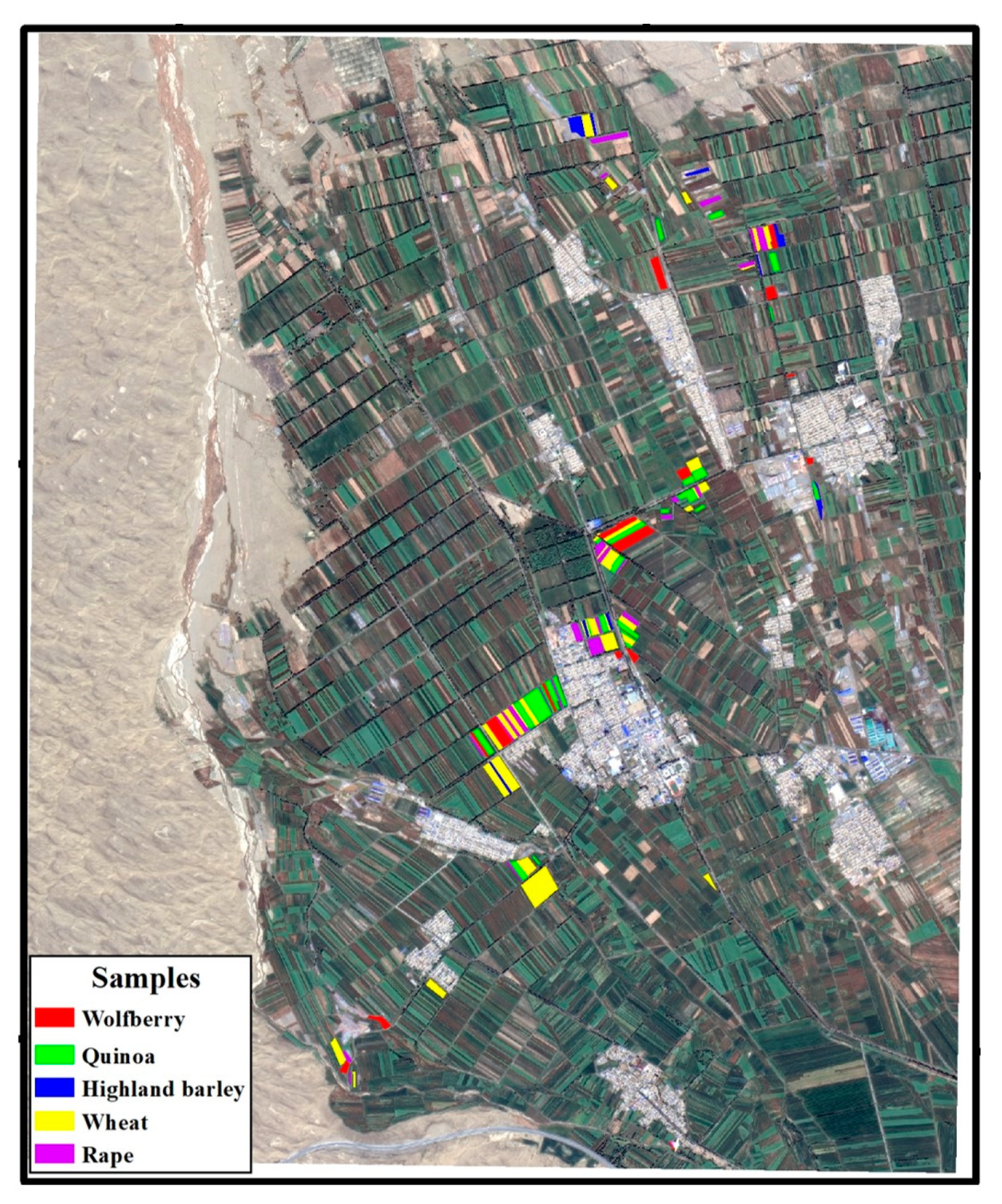
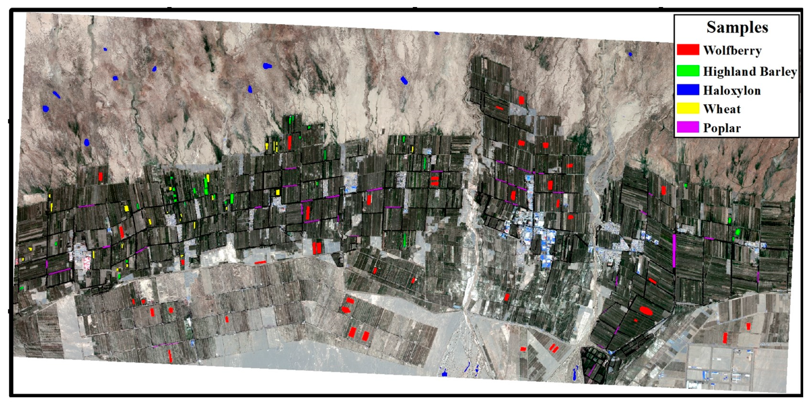
Based on research by Yang [50], in Site #1, the predominant crops included wheat, quinoa, and rape, alongside specialty crops like wolfberry and quinoa. In Site #2, wolfberry was the primary crop, with smaller areas devoted to wheat and quinoa cultivation. Other vegetation types comprised shelterbelt poplar and haloxylon. Field surveys were undertaken at Site #1 and Site #2 during 20–22 August 2021 and 8–10 August 2020, respectively. These surveys aimed to corroborate the crop types within the study area by leveraging existing data and to meticulously select suitable training samples. In parallel, high-resolution remote sensing images were utilized as references for the selection of training and validation samples corresponding to each vegetation type. Sample regions of crops were delineated at the field level. The distribution of field samples at Site #1 and Site #2 is depicted in Figure 3 and Figure 4, respectively. The numbers of training samples and validation samples are compared for each crop/vegetation type in Table 2. The training and validation samples are randomly selected in a 1:1 ratio at the field level, ensuring a balanced spatial distribution of samples. Furthermore, 32 and 36 background (construction and bare land) sample regions were collected for Sites #1 and #2.

2.3.2. Multisource Remote Sensing Features

The study extracted multisource remote sensing features, comprising reflectance data from Gaofen-6 post-atmospheric correction (GF), time series of VV/VH backscattering coefficients (SAR) from Sentinel-1 after noise removal and terrain correction, and time series of vegetation indices (VI) and biophysical variables (BP) computed from Sentinel-2 data.
  • Vegetation indices (VI)
Vegetation indices serve as vital tools to extract vegetation information from remote sensing data, aiding in the differentiation between vegetated and non-vegetated regions. They capture variations in greenness and vegetation density across diverse crops and vegetation types. Time series of vegetation indices can depict the growth cycle and seasonal fluctuations of crops, facilitating the differentiation of various crop types [22]. The most frequently utilized vegetation indices for crop classification are the Normalized Difference Vegetation Index (NDVI) [21], Soil-Adjusted Vegetation Index (SAVI) [51] and Ratio Vegetation Index (RVI) [52]. The formulas for the NDVI, SAVI, and RVI are provided below.
N D V I = ( ρ ( N i r ) ρ ( R e d ) ) / ( ρ ( N i r ) + ρ ( R e d ) )  
S A V I = ( 1 + L ) × ( ρ ( N i r ) ρ ( R e d ) ) / ( ρ ( N i r ) + ρ ( R e d ) + L )
R V I = ρ ( N i r ) / ρ ( R e d )
where ρ ( N i r ) and ρ ( R e d ) represent the reflectance values of Sentinel-2 bands 8 and 4, respectively. L stands as a correction factor, varying from 0 for extensive vegetation cover to 1 for minimal vegetation cover. The value most frequently employed is 0.5, signifying intermediate vegetation coverage.
  • Biophysical variables (BP)
The Leaf Area Index (LAI), the Fraction of Absorbed Photosynthetically Active Radiation (FAPAR), the Fraction of Vegetation Cover (FCOVER), the chlorophyll content in the leaf (Cab), and the canopy water content (CW) were extracted and employed for crop classification. These indices were computed from Sentinel-2 data using the Biophysical Processor module of the SNAP 9.0 platform, as proposed by Weiss et al. [53]. Neural networks were employed to estimate Sentinel-2 biophysical variables, enabling the algorithm’s broad applicability without specific inputs tailored to individual land cover types. This feature facilitates its global extension for vegetation biophysical variable retrieval. Hu et al. [54] assessed the Biophysical Processor’s performance, employing ground observations from diverse landscapes and reference maps and following consistent measurement criteria. The achieved accuracy consistently surpassed 87% for the LAI, FAPAR, and FCOVER. The LAI, FAPAR, FCOVER, Cab, and CW offer insights into various aspects of vegetation, including its structure, photosynthetic activity, coverage, and physiological condition. These variables serve to differentiate between distinct types of vegetation. The LAI represents the total leaf area of plants relative to the land area they cover. Plant species exhibit diverse leaf morphology, size, and arrangement, resulting in variations in total leaf areas [55]. Furthermore, leaf number and size undergo changes throughout the crop growing season, leading to periodic fluctuations in the LAI [56]. The FAPAR signifies the fraction of photosynthetically active radiation absorbed by vegetation. Variations in the FAPAR among different vegetation types mirror their efficiency in utilizing light energy and growth status, with denser vegetation typically exhibiting higher FAPAR values [57]. Variations in the FCOVER among different vegetation types reflect their spatial distribution and density [57]. The Cab can discern variations in chlorophyll content among different vegetation types. The CW pertains to the water content in the vegetation canopy, and differences in the canopy water content among distinct vegetation types indicate their water utilization and regulatory characteristics [58].

2.3.3. Feature Fusion

To investigate the performance of diverse remote sensing features and their combinations in crop/vegetation classification, we integrated multiple remote sensing features to create four individual feature sets, as well as a feature-fused set. The individual feature sets are as follows: (1) the SAR feature set, encompassing 12 periods of backscatter coefficients (VV and VH), totaling 24 features; (2) the GF feature set, incorporating the reflectance of 4 spectral bands: blue, green, red, and near-infrared; (3) the VI feature set, encompassing 12 periods of NDVI, RVI, and SAVI, constituting a total of 36 features; and (4) the BP feature set, comprising 12 periods of LAI, Cab, CWC, FAPAR, and FVC, culminating in 60 features. The feature-fused set is designated as (5) the SAR + GF + VI + BP feature set, an amalgamation of the four aforementioned feature sets, which results in a cumulative 124 features.

2.3.4. Classifiers

Prior research has demonstrated that conventional supervised classification algorithms, including Random Forests (RFs), Support Vector Machines (SVMs), and Maximum Likelihood (ML), along with deep learning algorithms such as Convolutional Neural Networks (CNNs), U-Net, and Long Short-Term Memory Networks (LSTMs), are widely employed in remote sensing crop classification [22,24,28,30,32]. In this study, the crop/vegetation classification employed ML, SVM, RF, and U-Net algorithms. ML is the most widely used classifier with remote sensing data and serves as the reference classifier in most of the related literature [59]. Using the Maximum Likelihood supervised classification module in ENVI 5.6, crop/vegetation image classification was conducted for two study areas, with a probability threshold set at 0.1. The SVM algorithm utilized a radial basis function (RBF) as its kernel for computation. Two parameters were required for the experiments: one for the penalty parameter, C, (indicating the magnitude of errors) and the other for the kernel function parameter, γ [20]. These parameters were obtained through 10-fold cross-validation of reference sample data. In the SVM crop/vegetation classification, the parameters C and γ for Site #1 and Site #2 were, respectively, set to 30 and 0.01 and 35 and 0.012. The RF algorithm, introduced by Breiman [60], is an integrated image classification method. The number of decision trees is a critical parameter in RFs, affecting both the classification accuracy and efficiency [61]. To balance between accuracy and time efficiency, we set the number of decision trees to 120 for Site #1 and 100 for Site #2 for crop classification. Additionally, the parameter max_features was uniformly set to 8 for both study sites. The U-Net network employed in this study shares the same kernel function size, stride, and activation function of the convolutional layer, pooling layer, and deconvolution layer as the network proposed by Ronneberger [62]. Considering the research area and data characteristics, the U-Net network was structured with four convolutional layers (256 × 256, 128 × 128, 64 × 64, 32 × 32) and three deconvolution layers (64 × 64, 128 × 128, 256 × 256). Moreover, to mitigate overfitting, a dropout layer was added after each Up-convolutional layer in the decoder, randomly deactivating 50% of the neurons.

2.3.5. Decision Fusion Strategies

The decision fusion of crop/vegetation classification outcomes was executed using Majority Voting (MV) [63], the Enhanced Overall Accuracy Index (E-OAI), and the OAI based Majority Voting (OAI-MV) strategies. OAI-MV is introduced as an innovative Majority Voting strategy, while the E-OAI represents a refined approach built upon the foundation of the Overall Accuracy Index (OAI) strategy [48].
  • Majority voting (MV)
The MV strategy adheres to the principle of “one person, one vote,” where equal weight coefficients are assigned to the classification outcomes of each participating classifier in the decision fusion process [63]. This guarantees uniform voting weights for all classifier results. The decision fusion rule is outlined below:
N ( j ) = i = 1 n I ( ω i = j )
In the formula, I is an indicator function, ω represents each classification class label, n represents the number of classifiers, and N ( j ) is the number of classification instances for the jth class label.
  • Enhanced Overall Accuracy Index (E-OAI) voting strategy
OAI strategy is a pooling-based decision fusion mapping process that harnesses various data sources and classifiers to establish pixel-level decision weights. This is achieved by considering accuracy metrics, including the overall accuracy (OA), the Kappa coefficient (Kappa), and the Class-specific Classification Accuracy [48]. The algorithm comprises the subsequent steps:
(1) Performing crop/vegetation classification using multisource remote sensing data and multiple classifiers.
Given that I i   ( i = 1 , 2 , , m ) denotes the data sources and f j   ( j = 1 , 2 , , n ) signifies the classifiers, the crop/vegetation classification was executed using n classifiers across m input data sources, leading to the generation of m × n classification outcomes.
I i f j C I i f j
In Equation (5), C I i f j denotes the classification result of the jth classifier for the ith data source.
(2) Accuracy assessments of the classification results.
Accuracy assessments were conducted for various classification results ( C I i f j ). Let C A i j be the class-specific accuracy of the ith data source with the jth classifier for the target class to be classified, and O A i j along with δ i j represent the OA and Kappa, respectively, of the classification result stemming from the mode of the ith data source and the jth classifier.
(3) Constructing the OAI and conducting decision fusion on diverse classification results.
Pal et al. [48] constructed the OAI for each classification result and each target class to be classified as follows:
O A I i j = C A i j × O A i j × δ i j
In Equation (6), Pal et al. [48] introduced O A I i j , where C A i j specifically refers to the producer’s accuracy (PA) of the classified type obtained from the classification result of the ith data source utilizing the jth classifier. Given the multitude of class-specific accuracy evaluation indicators and the various ways they can be combined, our aim is to thoroughly examine the impact of constructing OAIs on the classification accuracy of decision fusion. In light of this, we redefined O A I i j into eight distinct types of OAIs within the framework of E-OAI strategy:
O A I 1 i j = C P A i j × O A i j × δ i j
O A I 2 i j = C U A i j × O A i j × δ i j
O A I 3 i j = C P A i j × C U A i j × O A i j × δ i j
O A I 4 i j = C P A i j × O A i j
O A I 5 i j = C U A i j × O A i j
O A I 6 i j = C P A i j × C U A i j × O A i j
O A I 7 i j = C F i j × O A i j × δ i j
O A I 8 i j = C F i j × O A i j
Within these formulas, C P A i j , C U A i j , and C F i j represent the PA, users’ accuracy, and F1 score, respectively, for the classified crop/vegetation category by the ith data source and the jth classifier.
The calculation of O A I i j for each crop/vegetable type is undertaken for each classification result. Furthermore, an x × y × r matrix ( O A I x y r ) is created, where x and y denote the rows and columns of the matrix, corresponding to the row and column coordinates within the classified image, and r = i × j , representing the total number of classification results obtained using i data sources and j classifiers.
Subsequently, two new matrices of size x × y are calculated:
M a x _ l o c a t i o n ( x , y ) = a r g m a x r ( O A I x y r )
M a x _ O A I ( x , y ) = m a x r ( O A I x y r )
where a r g m a x r is a function that returns the index corresponding to the maximum value in the r dimensions of the matrix, O A I x y r . In this context, it helps identify the position of the maximum OAI value among the r classification results for each pixel ( x , y ). And m a x r is a function that selects the maximum value from the set of r OAI values for each pixel.
Based on the value of each pixel ( x , y ) in M a x _ l o c a t i o n ( x , y ) , we ascertain its corresponding classification result r   ( 1 , 2 , , i × j ) . Subsequently, we establish the decision fusion classification category of pixel ( x , y ) according to the crop/vegetation classification category of this result at pixel ( x , y ) .
(4) Optimizing classification accuracy.
The decision fusion classification result’s accuracy is assessed, and the OAI ( M a x _ O A I ( x , y ) ) is computed for each pixel ( x , y ) . A comparison was made between M a x _ O A I ( x , y ) and M a x _ O A I ( x , y ) for each pixel. The post-decision fusion class assignment of a pixel is accepted only if the index value, M a x _ O A I ( x , y ) , is greater than M a x _ O A I ( x , y ) . Pal et al. [48] utilized a 3 × 3 pixel window for maximal frequency filtering during classification result optimization in their study. However, to prevent this operation’s influence on comparing different decision fusion strategies, our study omitted this filtering step.
(5) Optimization of OAI strategy
To ascertain the influence of various OAIs on the precision of the OAI strategy, individual decision fusion is performed employing each of the eight distinct OAIs outlined in step (3). This procedure yields eight distinct decision fusion results. Following this, an accuracy evaluation is undertaken on these results to identify the classification outcome demonstrating the highest overall accuracy.
  • Overall Accuracy Index based Majority Voting (OAI-MV)
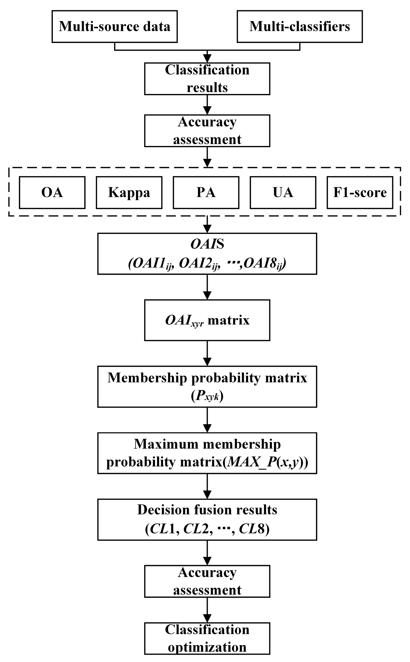
The OAI-MV approach involves computing the OAI for each pixel ( O A I i j ( x , y ) ), signifying dissimilarities in classification performance among distinct classification results for various crop/vegetable types. These calculated OAI values are then used to assign weights to each pixel, reflecting their importance in the voting procedure. Subsequently, the majority voting strategy is applied to integrate multiple classification outcomes using the assigned weights. The procedural outline of OAI-MV is depicted in Figure 5. While the exact calculation of O A I i j ( x , y ) is omitted in this section, the algorithmic framework of OAI-MV is outlined below:
(1) Calculating the membership probability matrix
Following the creation of the matrix ( O A I x y r ), an x × y × k membership probability matrix, P , is determined as follows:
P x y k = 1 r O A I x y r · δ ( k C l a s s x y r )
where k   ( 1 , 2 , , n ) represents classes of crop/vegetation. O A I x y r denotes the OAI value of the r th classification result at pixel ( x , y ) . C l a s s x y r represents the classification category of the r th classification result at pixel ( x , y ) . δ ( k C l a s s x y r ) is the Kronecker delta function, which equals 1 when k equals C l a s s x y r and 0 otherwise. P x y k signifies the membership probability of the pixel located at ( x , y ) belonging to the kth class of crop/vegetation.
(2) Majority Voting of membership probability
The computation of the maximum membership probability matrix ( M A X _ P ( x , y ) ) is as follows:
M A X _ P ( x , y ) = a r g m a x k ( P x y k )
where a r g m a x k is a function that returns the index corresponding to the maximum value in the k dimensions of the matrix P x y k . Each pixel is classified into the corresponding crop/vegetation type of M A X _ P ( x , y ) .
(3) Optimizing classification accuracy.
The decision fusion results of OAI-MV are optimized using the same method as the OAI for optimization. Due to the classification accuracy uncertainty associated with the eight OAIs ( O A I 1 i j ~ O A I 8 i j ), separate decision fusion is carried out using each of the eight OAIs in step (1)~(2). This process generated eight decision fusion outcomes (CL1~CL8). Subsequently, an accuracy assessment is conducted on these outcomes to determine the OAI-MV classification result with the highest OA.

2.3.6. Classification Scenarios

To examine the efficacy of various remote sensing feature sets, classifiers, and decision fusion strategies in crop/vegetation classification, we constructed 20 distinct crop/vegetation classification models for the five feature sets employing four classifiers, including ML, RFs, SVMs, and U-Net (refer to Table 3, S1~S20). The classification outcomes from S1 to S20 were consolidated into 6 groups. Subsequently, the three decision fusion strategies, MV, E-OAI, and OAI-MV, were employed to fuse each group of the classification results (refer to Table 3, S21~S38).

2.3.7. Accuracy Assessment

The study employed the confusion matrix method to assess the pixel-based classification accuracy [49,64]. The OA and Kappa served as evaluation metrics for the classifier’s overall accuracy. Additionally, the PA, UA, and F1 score (F1) were utilized to evaluate class-specific accuracy. Accuracy assessment was conducted on both the crop/vegetation classification results of single classifiers and the decision fusion results. The OA represents the ratio of correctly classified pixels to the total number of classified pixels [64]. The PA refers to the ratio of the correctly classified pixels of a certain class to the total number of pixels in the validation samples of that class. The UA is the ratio of the correctly classified pixels of a certain class to the total number of pixels classified as that class [64]. The formulas for calculating the F1 score and Kappa coefficient are as follows:
F 1 s c o r e = 2 × P A × U A P A + U A
K a p p a =   w f o w f c n   w f c
In the formula,   w f o represents the proportion of correctly classified cells in the confusion matrix, and   w f c represents the proportion of classification errors caused by chance factors in the confusion matrix.

3. Results

3.1. Crop/Vegetation Classification of Different Feature Sets with Single Classifier

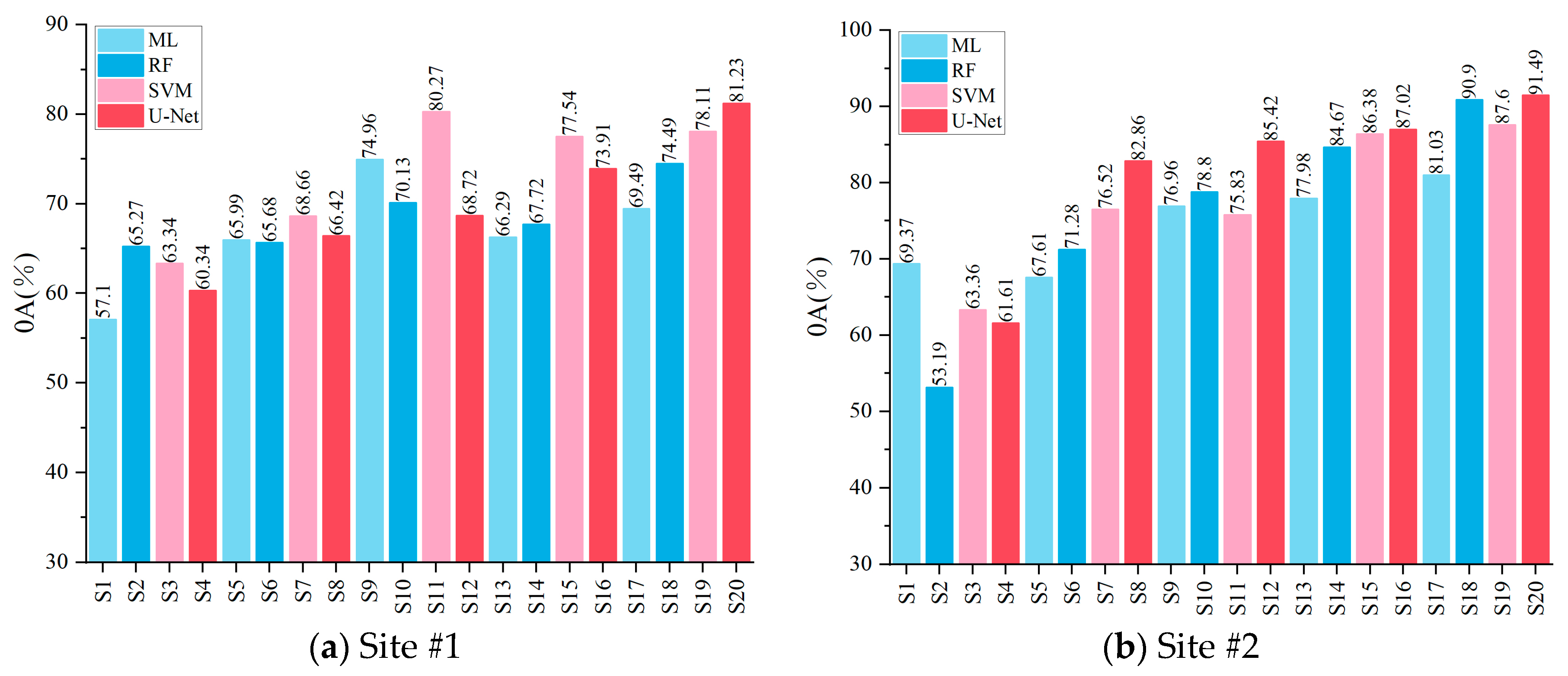
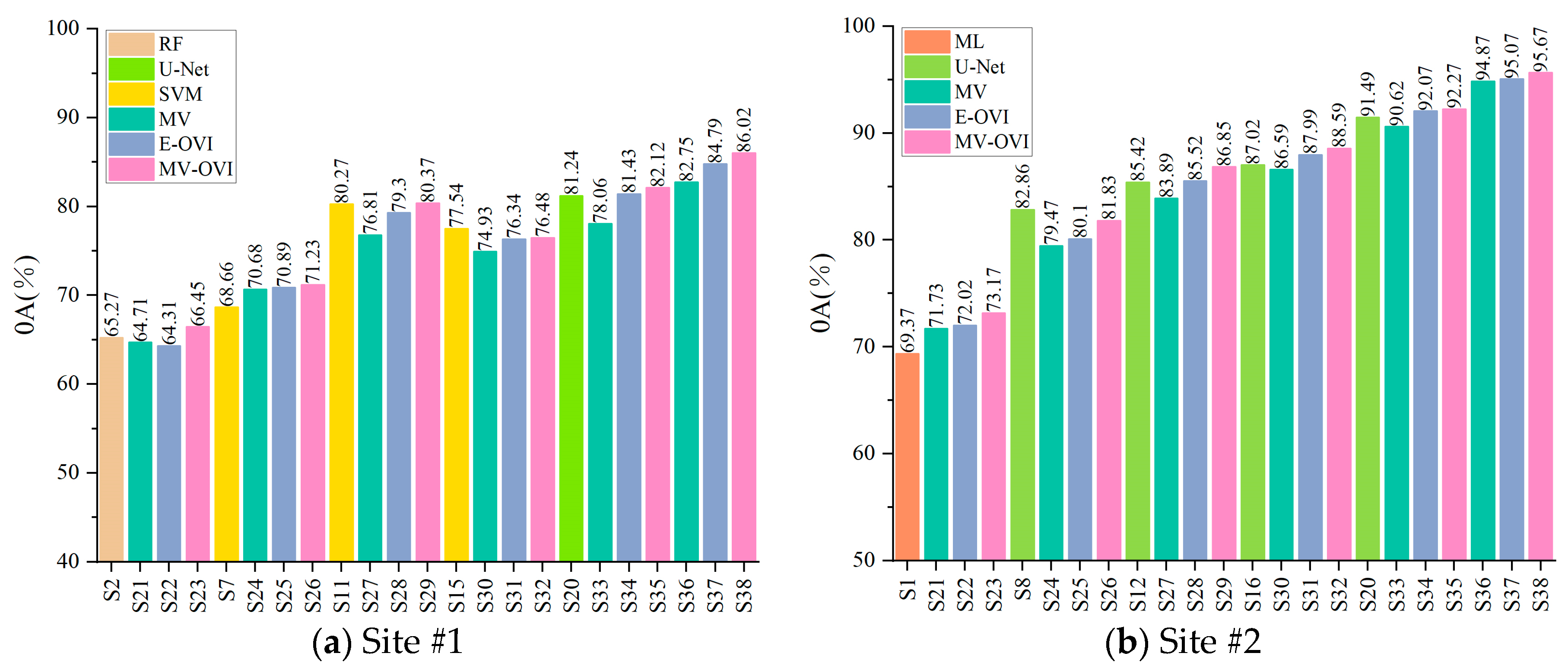
The overall accuracy (OA) of crop/vegetation classification varies across different feature sets when applying different classifiers (Figure 6). The feature-fused set (SAR + GF + VI + BP) achieved the highest OA of 81.23% and 91.49% for Site #1 and Site #2, respectively. Among the four independent feature sets, BP and VI exhibited higher OAs. The OAs for the BP feature set were 77.54% and 87.02% for Site #1 and Site #2, respectively. Similarly, the OAs for the VI feature set were 80.27% and 85.42% for Site #1 and Site #2. In contrast, the OA of the SAR feature set was the lowest, with values of 65.27% for Site #1 and 69.37% for Site #2. In terms of classifiers, the SVM achieved the highest OAs for GF, VI, and BP. U-Net and the RF demonstrated the highest OAs for SAR + GF + VI + BP and SAR, respectively, at Site #1. Notably, U-Net yielded the highest OAs for GF, VI, BP, and SAR + GF + VI + BP, while ML achieved the highest OA for SAR at Site #2.
Table 4 presents the PA, UA, and F1 scores for different crop/vegetation types across the various classification results. Distinct feature sets coupled with different classifiers exhibited varying performances concerning distinct crop/vegetation types. Regarding Site #1, the F1 score of wolfberry in S15 (BP with the SVM) surpassed that of other scenarios. S20 (SAR + GF + VI + BP with U-Net) achieved the highest F1 score for quinoa and highland barley, whereas for wheat, the F1 score in S11 (VI with the SVM) outperformed the other scenarios. Moreover, S7 (GF with the SVM) yielded the highest F1 score for rape at Site #1. As for Site #2, the F1 scores for wolfberry, highland barley, haloxylon, and wheat were most elevated in S20 (SAR + GF + VI + BP with U-Net). Conversely, the highest F1 score for poplar was attained in S18 (SAR + GF + VI + BP with the RF).

3.2. Crop/Vegetation Classification of Decision-Level Fusion

A comparison of the OAs for the different decision-level fusion scenarios is depicted in Figure 7. The proposed OAI-MV achieved the highest OA in the three decision-level fusion strategies for all the decision-level fusion experiments (S21~S38). OAI-MV, applied to all the classification results (S1~S20), achieved the highest OA of 86.02% and 95.67% for Site #1 and Site #2, respectively. However, the performance of the decision-level fusion strategies varied across different feature sets. For Site #1, MV, E-OAI, and OAI-MV improved the OA of the GF feature set by 2.02, 2.23, and 2.57 percent, respectively, compared to the GF scenarios with a single classifier. Additionally, E-OAI and OAI-MV slightly enhanced the OA of the SAR + GF + VI + BP feature set by 0.19 and 0.88 percent, respectively, compared to the single-classifier scenario of SAR + GF + VI + BP. Nevertheless, for the SAR and VI feature sets, only OAI-MV managed to improve the OA by 1.18 and 0.10 percent, respectively, compared to the single-classifier scenarios. In addition, for the BP feature set, MV, E-OAI and OAI-MV did not lead to an improvement in the OA. For Site #2, MV, E-OAI, and OAI-MV increased the OA of SAR (S1) by 1.93, 2.65, and 3.8 percent, respectively. Moreover, E-OAI and OAI-MV elevated the OA of the BP, VI, and SAR + GF + VI + BP feature sets by 0.97% and 1.57%, 0.1% and 1.43%, and 0.58% and 0.78%, respectively, compared to the single-classifier results, with the highest OA (S16, S12, and S20) for the feature sets.
Table 5 presents a comparison of the PA, UA, and F1 score for different crop/vegetation types in the decision-level fusion classification results. Concerning Site #1, S38, which integrated all the classification results through the OAI-MV strategy, the highest accuracy for wolfberry, quinoa, and highland barley was obtained, with F1 scores of 91.3%, 87.8%, and 89.7%, respectively. For wheat, S37, which combines all the classification results using the E-OAI strategy, the highest F1 score of 86.4% was obtained, while MV, combining the classification results of GF, achieved the highest F1 score (80.3%) for rape. On the other hand, at Site #2, S38, which amalgamated all the classification outcomes using the OAI-MV strategy, attained the highest accuracy for wolfberry, highland barley, haloxylon, wheat, and poplar, with F1 scores of 96.8%, 86.8%, 95.2%, 97.4%, and 96.9%, respectively. Notably, the accuracy of crop/vegetation classification was consistently higher at Site #2 compared to Site #1.
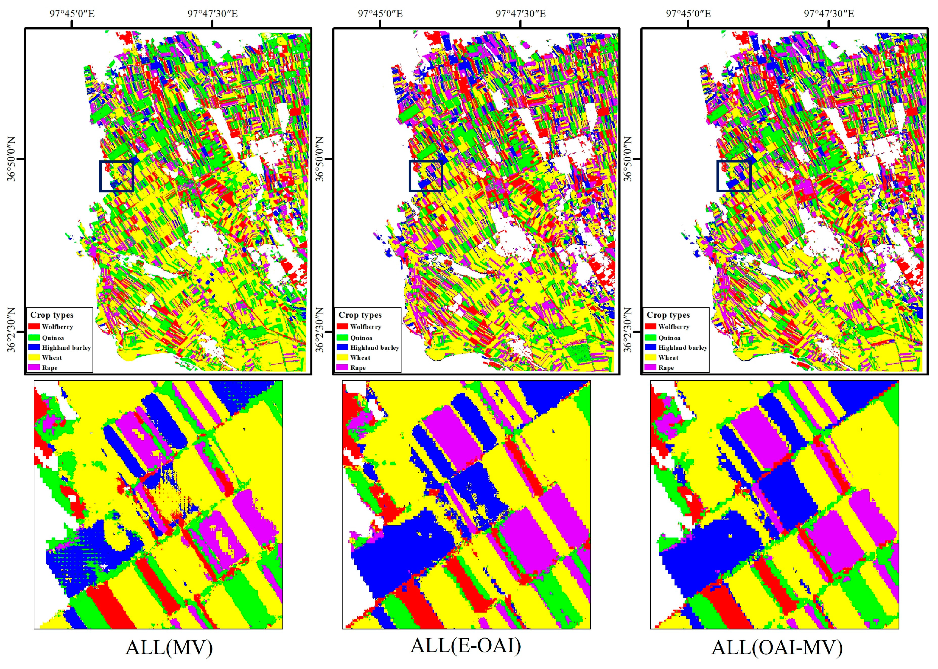
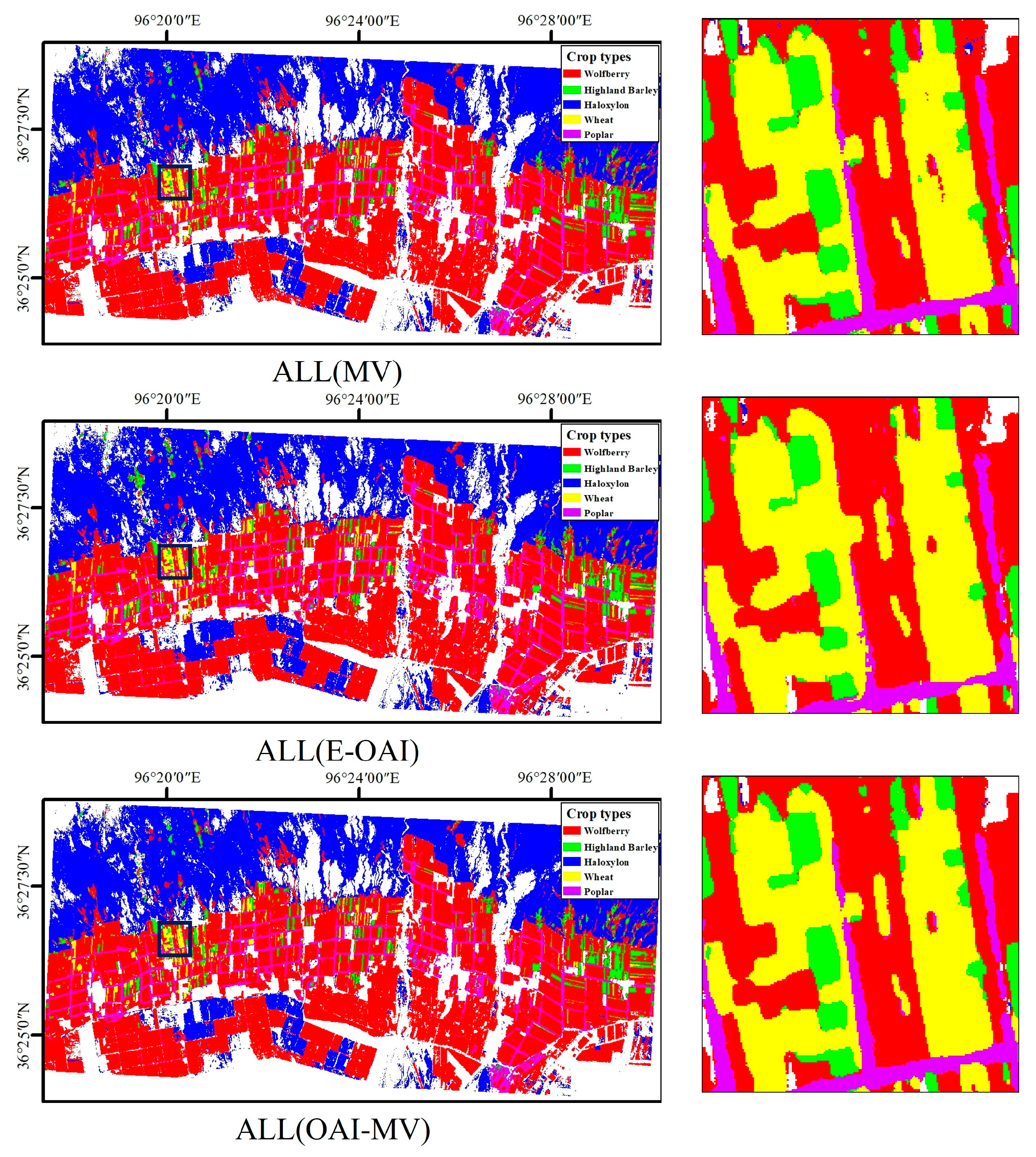
The decision-level-fused classification images for all the classification results using MV, E-OAI, and OAI-MV (S36, S37, and S38) are presented in Figure 8 (Site #1) and Figure 9 (Site #2). It is evident that OAI-MV yields superior performance in classifying crop/vegetation types. In Figure 8, a notable number of pixels within the rape and highland barley regions were erroneously categorized as wheat in the MV outcome, which contrasts with the results obtained from E-OAI and OAI-MV. Moreover, in the E-OAI outcome, a higher count of pixels in the highland barley region were inaccurately identified as wheat compared to OAI-MV. Figure 9 demonstrates that the MV outcome displayed more misclassified pixels within the wheat region compared to the E-OAI and OAI-MV outcomes. Furthermore, the E-OAI result exhibited a greater inability to identify poplar pixels compared to OAI-MV.

4. Discussion

4.1. Comparison of Crop/Vegetation Classification Performance with Different Feature Sets and Classifiers

Five distinct remote sensing feature sets were employed for crop/vegetation-type classification: SAR, GF, VI, BP, and SAR + GF + VI + BP. These feature sets were combined with four classifiers, ML, an SVM, a RF, and U-Net, to generate a total of 20 classification results. The classification results exhibited diverse performance trends among these feature sets in recognizing crop/vegetation types. Specifically, SAR yielded the lowest accuracy in crop/vegetation cover classification, with mean overall accuracy (OA) values of 61.51% for Site #1 and 61.88% for Site #2. These values were inferior to those achieved by the other optical feature sets. This conclusion aligns with findings reported by Chabalala et al. [20], Fathololoumi et al. [12], and Tuvdendorj et al. [22]. Chakhar et al. [21] demonstrated that optical remote sensing features were more crucial than radar features in crop/vegetation classification. Among the four feature sets (SAR, GF, VI, BP), the VI and BP feature sets achieved the highest mean OA values of 73.52% and 84.01% for Sites #1 and #2, respectively. In contrast, the GF feature set attained mean OA values of 66.69% and 74.57% for Sites #1 and #2, respectively, which were lower than those of the VI and BP feature sets. This discrepancy could be attributed to the fact that while GF features possess higher spatial resolution, the VI and BP feature sets exhibit superior spectral and temporal resolution. Spatial detail information, spectral information, and temporal variation information are all essential factors for delineating disparities among crops [4,8]. High-spatial-resolution data excel in capturing spatial intricacies arising from variations in plant morphology and canopy structure among different crops [25]. Meanwhile, spectral information and temporal variation information can highlight variations in physiological and biochemical traits, as well as differences in phenological patterns, across distinct crops [12]. The results of the classification experiments indicate that spectral information and temporal variation features bear greater significance in crop identification compared to spatial information. Zhang and Li [65] demonstrated that the accuracy of crop classification is relatively unaffected by spatial resolution when the image’s spatial resolution is finer than 60 m. In this study, the bands from Sentinel-2 used for calculating the VI and BP feature sets possessed spatial resolutions of 10 m or 20 m. Consequently, the image’s spatial resolution assumed a secondary significance among the factors influencing the crop classification accuracy in this investigation. It is important to highlight that, despite not being predominant in terms of the OA, the GF feature set exhibited strengths in identifying specific crop types. For instance, at Site #1, the GF feature set achieved the highest average F1 score of 0.781 for rape, outperforming the VI feature set with 0.650 and the BP feature set with 0.555. The feature-level fusion technique notably enhanced crop classification accuracy at both study sites. The SAR + GF + VI + BP feature set elevated the mean OA of crop classification by 2.39% and 3.74% for Site #1 and Site #2, respectively, along with enhancing the maximum OA by 3.70% and 4.46% for the respective sites. However, for specific crop categories, the individual feature sets displayed better recognition accuracy. For Site #1, compared to the SAR + GF + VI + BP feature set, the VI and BP feature sets demonstrated superior average F1 scores for wolfberry, while the GF feature set exhibited higher average F1 scores for rape. This phenomenon could be attributed to the influence of the high-dimensional feature fusion data, as suggested by the Hughes effect [66].
The classification performance of the four classifiers, namely ML, the SVM, the RF, and U-Net, varies when applied to different feature sets. Moreover, it is important to note that the recognition accuracy of different classifiers varies for different crops, even when considering the same feature sets. At Site #1, when U-Net was applied to GF, it yielded the highest F1 scores for wolfberry and highland barley. In the case of quinoa and rape, the SVM achieved the highest F1 scores, while the RF demonstrated the highest F1 scores for wheat. For Site #2, ML applied to SAR achieved the highest F1 scores for highland barley and haloxylon, while the SVM attained the highest F1 scores for wheat and poplar. And for wolfberry, the highest F1 score was achieved by U-Net. Notably, when the SAR + GF + VI + BP feature set was used and U-Net was applied, the best F1 scores for wolfberry, highland barley, and wheat were achieved. Additionally, the SVM and RF obtained the highest F1 score for haloxylon and poplar, respectively. It is essential to acknowledge that resource constraints resulted in a limited number of training samples for each crop/vegetation type in this study. This limitation notably affects deep learning algorithms like U-Net, which are highly dependent on the quantity of training samples. When different classification algorithms were tested on the same feature set, U-Net attained the highest OA in 5 out of 10 comparative experiments for crop classification at Site #1 and Site #2. This illustrates that even under conditions of restricted training samples, the U-Net algorithm retains certain advantages over traditional classification algorithms.
Distinct classifiers and diverse feature sets possess inherent strengths in discerning between specific crop/vegetation types. Consequently, employing suitable decision fusion strategies to leverage the varied benefits of different feature sets and classifiers is essential for improving the overall classification accuracy.

4.2. Crop/Vegetation Classification Performance of Different Decision Fusion Strategies

The MV strategy is a prominent decision-level fusion approach in remote sensing crop classification, significantly bolstering classification accuracy across diverse research endeavors [12,14]. Nevertheless, in the context of this study, the MV strategy did not uniformly enhance the precision of crop classification; it yielded improved classification accuracy in merely 4 out of the 12 decision fusion experiments when compared to the classification results with a single classifier. In situations where considerable variations exist in the accuracy of distinct classification outcomes during the fusion process, MV often fails to deliver consistent improvements in classification accuracy [46,48]. Shen et al. [47] also noted the instability in the outcomes of the MV and weighted MV strategies in their study. The Overall Accuracy Index (OAI) strategy achieves decision-level fusion by amalgamating overall accuracy evaluation metrics (OA and Kappa) and a class-specific accuracy metric (PA) to construct the OAI. The OAI reflects the discrepancies in both the overall accuracy of classifiers and their ability in distinguishing between various classification categories. Pal et al. [48] substantiated the OAI’s superiority over MV in lithological classification involving multiple classifiers. In this study, we introduced seven supplementary OAIs to enhance the existing OAI strategy, resulting in the development of the E-OAI strategy. The findings revealed that out of the 12 decision fusion experiments conducted, the E-OAI strategy surpassed the individual classifiers in 8 experiments, achieving a higher OA. Additionally, in 11 out of the 12 experiments, the E-OAI strategy outperformed the MV strategy. The study introduced a novel decision fusion strategy named OAI-MV, which combined the majority voting decision strategy with the OAIs. Among the 12 experiments conducted, the fusion outcomes obtained through OAI-MV exhibited superior OA in comparison to both the MV and E-OAI strategies, underscoring the efficacy of OAI-MV. However, it is important to note that for the classification results of BP at Site #1 and GF at Site #2, none of the three decision fusion strategies succeeded in improving the classification accuracy. This suggests the variability and unpredictability inherent in decision fusion strategies [47,48]. It is important to acknowledge that while the proposed OAI-MV and E-OAI strategies have significantly improved crop classification accuracy, they involve more calculations for weight factors and demand more complex decision-making. For example, the addition of seven types of OAIs for computation and comparison, compared to the OAI strategy, complicates and lengthens the calculation process. Future research will delve into understanding how the quantity and accuracy disparities in the classification outcomes affect the efficacy of decision fusion, aiming to further enhance the effectiveness of such strategies.

4.3. Impact of Different OAIs on Classification Accuracy of OAI Strategy

Pal et al. [48] proposed an Overall Accuracy Index (OAI) strategy, utilizing metrics such as the OA, Kappa coefficients, and a class-specific accuracy metric (PA) for its calculation. Given the range of diverse class-specific accuracy metrics and their potential combinations, this study introduced seven additional OAIs. These OAIs were designed to provide a comprehensive assessment of classification accuracy. Subsequently, decision fusion experiments using the OAI strategy were conducted, utilizing classification outcomes obtained from diverse feature sets coupled with distinct classifiers. The objective was to assess the accuracy performance associated with the various OAIs (as shown in Table 6). Across various groups of decision fusion experiments within Site #1, the adoption of different OAIs resulted in a variance in the OA ranging from a minimum of 2.52% (for the VI feature set) to a maximum of 6.70% (for the GF feature set). Similarly, for site #2, the utilization of distinct OAIs led to variations in the OA spanning from 1.27% (for the GF feature set) to 7.06% (for the BP feature set). Among the eight distinct OAIs employed in the twelve decision fusion experiments within the two testing sites, OAI2 emerged as the top performer in six experiments, while OAI5 and OAI6 achieved the highest OA in two experiments each. Furthermore, OAI3 and OAI4 secured the highest OA in one group each. Notably, the OAI1 proposed in the original OAI strategy [48] did not yield the highest classification accuracy in any of the experiments.
Given the fluctuating impact of the OAIs on decision fusion classification accuracy, all eight OAIs were employed in fusing the classification outcomes within the enhanced OAI strategy. The outcome of the E-OAI strategy was determined by selecting the decision fusion result with the highest overall accuracy from the eight different OAIs. In comparison with the original OAI strategy, the E-OAI strategy resulted in an enhancement ranging from 0.33% to 6.02% in the OA of crop/vegetation classification for Site #1, while for Site #2, the improvement ranged from 0.17% to 6.28%. The experiment results reveal that none of the eight OAIs consistently attained the highest classification accuracy. Hence, the suggested E-OAI and OAI-MV strategies iteratively employed diverse OAIs for decision fusion to ensure stable enhancements in classification accuracy, albeit at the expense of increased computational complexity. Subsequently, research will delve deeper into the impact mechanisms of OAIs on decision fusion accuracy, aiming to further optimize the E-OAI and OAI-MV strategies.

5. Conclusions

Accurately acquiring spatial information regarding crop distribution is fundamental for enabling precise agricultural management and ensuring food security. This study introduces novel decision fusion strategies, namely E-OAI and OAI-MV, to amalgamate the classification results of crops/vegetation from diverse remote sensing features and classifiers. After conducting the experiments and analysis, the study reached the following conclusions:
(1) Combining multisource remote sensing features effectively enhanced crop/vegetation identification accuracy. Employing U-Net on feature-combined sets resulted in the highest overall accuracy for both Site #1 and Site #2 in the single-classifier experiments.
(2) The different remote sensing features and classifiers demonstrated varying performance in identifying different crop/vegetation types.
(3) The proposed E-OAI strategy significantly enhanced the classification accuracy of the decision fusion crop/vegetation classification compared to the original OAI strategy.
(4) The proposed OAI-MV strategy consistently achieved the highest classification accuracy across all the decision fusion experiments, leading to heightened precision in crop/plant classification.
For future research endeavors, we intend to delve deeper into elucidating the influence mechanisms of various types of OAIs on decision fusion accuracy, thereby enhancing the precision of crop classification through the utilization of multisource remote sensing data and multiple classifiers. Additionally, our agenda includes optimizing the algorithmic structure to enhance computational efficiency.

Author Contributions

Conceptualization, S.S. and Z.Z.; methodology, S.S. and T.Z.; software, S.S., W.L. and L.T.; validation, Z.Z. and T.Z.; writing—original draft, S.S. and Z.Z.; writing—review and editing, Z.Z., S.S., X.D. and J.W.; visualization, J.W. and S.S.; funding acquisition, Z.Z. and S.S. All authors have read and agreed to the published version of the manuscript.

Funding

This research was funded by Scientific research project of Wuhan Polytechnic University (Grant 2023RZ025) and the Key Laboratory of the Northern Qinghai–Tibet Plateau Geological Processes and Mineral Resources (Grant 2019-KZ-01).

Data Availability Statement

The data presented in this study are available upon request from the corresponding author.

Acknowledgments

The authors would like to thank the European Space Agency (ESA) for providing the data used in this study. The authors extend gratitude to Jinxi Yao and Chengzhi Xiao for their assistance in field data collection.

Conflicts of Interest

Author Tian Zhang was employed by the company China Communications Construction Company second Highway Consultants Limited Company. The remaining authors declare that the research was conducted in the absence of any commercial or financial relationships that could be construed as a potential conflict of interest.

References

  1. Alexandratos, N. How to Feed the World in 2050. Proc. Tech. Meet. Experts 2009, 1–32. Available online: https://www.fao.org/fileadmin/templates/wsfs/docs/expert_paper/How_to_Feed_the_World_in_2050.pdf (accessed on 25 April 2024).
  2. Fan, J.; Zhang, X.; Zhao, C.; Qin, Z.; De Vroey, M.; Defourny, P. Evaluation of Crop Type Classification with Different High Resolution Satellite Data Sources. Remote Sens. 2021, 13, 911. [Google Scholar] [CrossRef]
  3. Futerman, S.I.; Laor, Y.; Eshel, G.; Cohen, Y. The Potential of Remote Sensing of Cover Crops to Benefit Sustainable and Precision Fertilization. Sci. Total Environ. 2023, 891, 164630. [Google Scholar] [CrossRef]
  4. Pluto-Kossakowska, J. Review on Multitemporal Classification Methods of Satellite Images for Crop and Arable Land Recognition. Agriculture 2021, 11, 999. [Google Scholar] [CrossRef]
  5. Sishodia, R.P.; Ray, R.L.; Singh, S.K. Applications of Remote Sensing in Precision Agriculture: A Review. Remote Sens. 2020, 12, 3136. [Google Scholar] [CrossRef]
  6. Zhang, C.; Marzougui, A.; Sankaran, S. High-Resolution Satellite Imagery Applications in Crop Phenotyping: An Overview. Comput. Electron. Agric. 2020, 175, 105584. [Google Scholar] [CrossRef]
  7. Sedighi, A.; Hamzeh, S.; Firozjaei, M.K.; Goodarzi, H.V.; Naseri, A.A. Comparative Analysis of Multispectral and Hyperspectral Imagery for Mapping Sugarcane Varieties. PFG—J. Photogramm. Remote Sens. Geoinf. Sci. 2023, 91, 453–470. [Google Scholar] [CrossRef]
  8. Zhao, L.; Li, F.; Chang, Q. Review on Crop Type Identification and Yield Forecasting Using Remote Sensing. Trans. Chin. Soc. Agric. Mach. 2023, 54, 1–19. [Google Scholar]
  9. Wan, S.; Chang, S.-H. Crop Classification with WorldView-2 Imagery Using Support Vector Machine Comparing Texture Analysis Approaches and Grey Relational Analysis in Jianan Plain, Taiwan. Int. J. Remote Sens. 2019, 40, 8076–8092. [Google Scholar] [CrossRef]
  10. Hively, W.D.; Shermeyer, J.; Lamb, B.T.; Daughtry, C.T.; Quemada, M.; Keppler, J. Mapping Crop Residue by Combining Landsat and WorldView-3 Satellite Imagery. Remote Sens. 2019, 11, 1857. [Google Scholar] [CrossRef]
  11. Orynbaikyzy, A.; Gessner, U.; Conrad, C. Crop Type Classification Using a Combination of Optical and Radar Remote Sensing Data: A Review. Int. J. Remote Sens. 2019, 40, 6553–6595. [Google Scholar] [CrossRef]
  12. Fathololoumi, S.; Firozjaei, M.K.; Li, H.; Biswas, A. Surface Biophysical Features Fusion in Remote Sensing for Improving Land Crop/Cover Classification Accuracy. Sci. Total Environ. 2022, 838, 156520. [Google Scholar] [CrossRef] [PubMed]
  13. Yuan, Y.; Lin, L.; Zhou, Z.-G.; Jiang, H.; Liu, Q. Bridging Optical and SAR Satellite Image Time Series via Contrastive Feature Extraction for Crop Classification. ISPRS J. Photogramm. Remote Sens. 2023, 195, 222–232. [Google Scholar] [CrossRef]
  14. Ghazaryan, G.; Dubovyk, O.; Löw, F.; Lavreniuk, M.; Kolotii, A.; Schellberg, J.; Kussul, N. A Rule-Based Approach for Crop Identification Using Multi-Temporal and Multi-Sensor Phenological Metrics. Eur. J. Remote Sens. 2018, 51, 511–524. [Google Scholar] [CrossRef]
  15. Xu, L.; Zhang, H.; Wang, C.; Zhang, B.; Liu, M. Crop Classification Based on Temporal Information Using Sentinel-1 SAR Time-Series Data. Remote Sens. 2019, 11, 53. [Google Scholar] [CrossRef]
  16. Moumni, A.; Oujaoura, M.; Ezzahar, J.; Lahrouni, A. A New Synergistic Approach for Crop Discrimination in a Semi-Arid Region Using Sentinel-2 Time Series and the Multiple Combination of Machine Learning Classifiers. J. Phys. Conf. Ser. 2021, 1743, 012026. [Google Scholar] [CrossRef]
  17. Gao, H.; Wang, C.; Wang, G.; Fu, H.; Zhu, J. A Novel Crop Classification Method Based on ppfSVM Classifier with Time-Series Alignment Kernel from Dual-Polarization SAR Datasets. Remote Sens. Environ. 2021, 264, 112628. [Google Scholar] [CrossRef]
  18. Rußwurm, M.; Courty, N.; Emonet, R.; Lefèvre, S.; Tuia, D.; Tavenard, R. End-to-End Learned Early Classification of Time Series for in-Season Crop Type Mapping. ISPRS J. Photogramm. Remote Sens. 2023, 196, 445–456. [Google Scholar] [CrossRef]
  19. Htitiou, A.; Boudhar, A.; Lebrini, Y.; Hadria, R.; Lionboui, H.; Benabdelouahab, T. A Comparative Analysis of Different Phenological Information Retrieved from Sentinel-2 Time Series Images to Improve Crop Classification: A Machine Learning Approach. Geocarto Int. 2020, 37, 1426–1449. [Google Scholar] [CrossRef]
  20. Chabalala, Y.; Adam, E.; Ali, K.A. Machine Learning Classification of Fused Sentinel-1 and Sentinel-2 Image Data towards Mapping Fruit Plantations in Highly Heterogenous Landscapes. Remote Sens. 2022, 14, 2621. [Google Scholar] [CrossRef]
  21. Chakhar, A.; Hernández-López, D.; Ballesteros, R.; Moreno, M.A. Improving the Accuracy of Multiple Algorithms for Crop Classification by Integrating Sentinel-1 Observations with Sentinel-2 Data. Remote Sens. 2021, 13, 243. [Google Scholar] [CrossRef]
  22. Tuvdendorj, B.; Zeng, H.; Wu, B.; Elnashar, A.; Zhang, M.; Tian, F.; Nabil, M.; Nanzad, L.; Bulkhbai, A.; Natsagdorj, N. Performance and the Optimal Integration of Sentinel-1/2 Time-Series Features for Crop Classification in Northern Mongolia. Remote Sens. 2022, 14, 1830. [Google Scholar] [CrossRef]
  23. Fathololoumi, S.; Firozjaei, M.K.; Biswas, A. An Innovative Fusion-Based Scenario for Improving Land Crop Mapping Accuracy. Sensors 2022, 22, 7428. [Google Scholar] [CrossRef] [PubMed]
  24. Al-Awar, B.; Awad, M.M.; Jarlan, L.; Courault, D. Evaluation of Nonparametric Machine-Learning Algorithms for an Optimal Crop Classification Using Big Data Reduction Strategy. Remote Sens. Earth Syst. Sci. 2022, 5, 141–153. [Google Scholar] [CrossRef]
  25. Xia, T.; He, Z.; Cai, Z.; Wang, C.; Wang, W.; Wang, J.; Hu, Q.; Song, Q. Exploring the Potential of Chinese GF-6 Images for Crop Mapping in Regions with Complex Agricultural Landscapes. Int. J. Appl. Earth Obs. Geoinf. 2022, 107, 102702. [Google Scholar] [CrossRef]
  26. Chabalala, Y.; Adam, E.; Ali, K.A. Exploring the Effect of Balanced and Imbalanced Multi-Class Distribution Data and Sampling Techniques on Fruit-Tree Crop Classification Using Different Machine Learning Classifiers. Geomatics 2023, 3, 70–92. [Google Scholar] [CrossRef]
  27. Laban, N.; Abdellatif, B.; Ebeid, H.M.; Shedeed, H.A.; Tolba, M.F. Machine Learning for Enhancement Land Cover and Crop Types Classification. In Machine Learning Paradigms: Theory and Application; Hassanien, A.E., Ed.; Studies in Computational Intelligence; Springer International Publishing: Cham, Switzerland, 2019; pp. 71–87. ISBN 978-3-030-02357-7. [Google Scholar]
  28. Agilandeeswari, L.; Prabukumar, M.; Radhesyam, V.; Phaneendra, K.L.N.B.; Farhan, A. Crop Classification for Agricultural Applications in Hyperspectral Remote Sensing Images. Appl. Sci. 2022, 12, 1670. [Google Scholar] [CrossRef]
  29. Ji, S.; Zhang, C.; Xu, A.; Shi, Y.; Duan, Y. 3D Convolutional Neural Networks for Crop Classification with Multi-Temporal Remote Sensing Images. Remote Sens. 2018, 10, 75. [Google Scholar] [CrossRef]
  30. Li, G.; Cui, J.; Han, W.; Zhang, H.; Huang, S.; Chen, H.; Ao, J. Crop Type Mapping Using Time-Series Sentinel-2 Imagery and U-Net in Early Growth Periods in the Hetao Irrigation District in China. Comput. Electron. Agric. 2022, 203, 107478. [Google Scholar] [CrossRef]
  31. Wei, S.; Zhang, H.; Wang, C.; Wang, Y.; Xu, L. Multi-Temporal SAR Data Large-Scale Crop Mapping Based on U-Net Model. Remote Sens. 2019, 11, 68. [Google Scholar] [CrossRef]
  32. Reuß, F.; Greimeister-Pfeil, I.; Vreugdenhil, M.; Wagner, W. Comparison of Long Short-Term Memory Networks and Random Forest for Sentinel-1 Time Series Based Large Scale Crop Classification. Remote Sens. 2021, 13, 5000. [Google Scholar] [CrossRef]
  33. He, T.; Xie, C.; Liu, Q.; Guan, S.; Liu, G. Evaluation and Comparison of Random Forest and A-LSTM Networks for Large-Scale Winter Wheat Identification. Remote Sens. 2019, 11, 1665. [Google Scholar] [CrossRef]
  34. Wang, X.; Zhang, J.; Xun, L.; Wang, J.; Wu, Z.; Henchiri, M.; Zhang, S.; Zhang, S.; Bai, Y.; Yang, S.; et al. Evaluating the Effectiveness of Machine Learning and Deep Learning Models Combined Time-Series Satellite Data for Multiple Crop Types Classification over a Large-Scale Region. Remote Sens. 2022, 14, 2341. [Google Scholar] [CrossRef]
  35. Solberg, A.H.S. Data Fusion for Remote Sensing Applications. In Signal and Image Processing for Remote Sensing; CRC Press: Boca Raton, FL, USA, 2006; pp. 249–271. [Google Scholar]
  36. Ban, Y.; Hu, H.; Rangel, I.M. Fusion of Quickbird MS and RADARSAT SAR Data for Urban Land-Cover Mapping: Object-Based and Knowledge-Based Approach. Int. J. Remote Sens. 2010, 31, 1391–1410. [Google Scholar] [CrossRef]
  37. Okamoto, K. International Journal of Estimation of Rice-Planted Area in the Tropical Zone Using a Combination of Optical and Microwave Satellite Sensor Data. Int. J. Remote Sens. 1999, 20, 1045–1048. [Google Scholar] [CrossRef]
  38. Soria-Ruiz, J.; Fernandez-Ordoñez, Y.; Woodhouse, I.H. Land-Cover Classification Using Radar and Optical Images: A Case Study in Central Mexico. Int. J. Remote Sens. 2010, 31, 3291–3305. [Google Scholar] [CrossRef]
  39. Kuncheva, L.I.; Bezdek, J.C.; Duin, R.P.W. Decision Templates for Multiple Classifier Fusion: An Experimental Comparison. Pattern Recognit. 2001, 34, 299–314. [Google Scholar] [CrossRef]
  40. Lam, L.; Suen, C.Y. Optimal Combinations of Pattern Classifiers. Pattern Recognit. Lett. 1995, 16, 945–954. [Google Scholar] [CrossRef]
  41. Ceccarelli, M.; Petrosino, A. Multi-Feature Adaptive Classifiers for SAR Image Segmentation. Neurocomputing 1997, 14, 345–363. [Google Scholar] [CrossRef]
  42. Grabisch, M. The Application of Fuzzy Integrals in Multicriteria Decision Making. Eur. J. Oper. Res. 1996, 89, 445–456. [Google Scholar] [CrossRef]
  43. Rogova, G. Combining the Results of Several Neural Network Classifiers. In Classic Works of the Dempster-Shafer Theory of Belief Functions; Yager, R.R., Liu, L., Eds.; Springer: Berlin, Heidelberg, 2008; pp. 683–692. ISBN 978-3-540-44792-4. [Google Scholar]
  44. Smits, P.C. Multiple Classifier Systems for Supervised Remote Sensing Image Classification Based on Dynamic Classifier Selection. IEEE Trans. Geosci. Remote Sens. 2002, 40, 801–813. [Google Scholar] [CrossRef]
  45. Benediktsson, J.A.; Chanussot, J.; Fauvel, M. Multiple Classifier Systems in Remote Sensing: From Basics to Recent Developments. In Multiple Classifier Systems; Haindl, M., Kittler, J., Roli, F., Eds.; Springer: Berlin, Heidelberg, 2007; pp. 501–512. [Google Scholar]
  46. Ye, Z.; Dong, R.; Chen, H.; Bai, L. Adjustive decision fusion approaches for hyperspectral image classification. J. Image Graph. 2021, 26, 1952–1968. [Google Scholar]
  47. Shen, H.; Lin, Y.; Tian, Q.; Xu, K.; Jiao, J. A Comparison of Multiple Classifier Combinations Using Different Voting-Weights for Remote Sensing Image Classification. Int. J. Remote Sens. 2018, 39, 3705–3722. [Google Scholar] [CrossRef]
  48. Pal, M.; Rasmussen, T.; Porwal, A. Optimized Lithological Mapping from Multispectral and Hyperspectral Remote Sensing Images Using Fused Multi-Classifiers. Remote Sens. 2020, 12, 177. [Google Scholar] [CrossRef]
  49. Foody, G.M.; Boyd, D.S.; Sanchez-Hernandez, C. Mapping a Specific Class with an Ensemble of Classifiers. Int. J. Remote Sens. 2007, 28, 1733–1746. [Google Scholar] [CrossRef]
  50. Yang, J. Study on the Evolution of Spatial Morphology of Farm Settlements in the Eastern Oasis of Qaidam Basin—A Case Study of Oasis Settlements in Xiangride and Nuomuhong River Basins; Xi’an University of Architecture and Technology: Xi’an, China, 2021. [Google Scholar]
  51. Niazmardi, S.; Homayouni, S.; Safari, A.; McNairn, H.; Shang, J.; Beckett, K. Histogram-Based Spatio-Temporal Feature Classification of Vegetation Indices Time-Series for Crop Mapping. Int. J. Appl. Earth Obs. Geoinf. 2018, 72, 34–41. [Google Scholar] [CrossRef]
  52. Teimouri, M.; Mokhtarzade, M.; Baghdadi, N.; Heipke, C. Fusion of Time-Series Optical and SAR Images Using 3D Convolutional Neural Networks for Crop Classification. Geocarto Int. 2022, 37, 15143–15160. [Google Scholar] [CrossRef]
  53. Weiss, M.; Baret, F.; Jay, S. S2ToolBox Level 2 Products: LAI, FAPAR, FCOVER. Version 2.1. 2020. Available online: https://step.esa.int/docs/extra/ATBD_S2ToolBox_L2B_V1.1.pdf (accessed on 25 April 2024).
  54. Hu, Q.; Yang, J.; Xu, B.; Huang, J.; Memon, M.S.; Yin, G.; Zeng, Y.; Zhao, J.; Liu, K. Evaluation of Global Decametric-Resolution LAI, FAPAR and FVC Estimates Derived from Sentinel-2 Imagery. Remote Sens. 2020, 12, 912. [Google Scholar] [CrossRef]
  55. Neinavaz, E.; Skidmore, A.K.; Darvishzadeh, R.; Groen, T.A. Retrieval of Leaf Area Index in Different Plant Species Using Thermal Hyperspectral Data. ISPRS J. Photogramm. Remote Sens. 2016, 119, 390–401. [Google Scholar] [CrossRef]
  56. González-Sanpedro, M.C.; Le Toan, T.; Moreno, J.; Kergoat, L.; Rubio, E. Seasonal Variations of Leaf Area Index of Agricultural Fields Retrieved from Landsat Data. Remote Sens. Environ. 2008, 112, 810–824. [Google Scholar] [CrossRef]
  57. Camacho, F.; Cernicharo, J.; Lacaze, R.; Baret, F.; Weiss, M. GEOV1: LAI, FAPAR Essential Climate Variables and FCOVER Global Time Series Capitalizing over Existing Products. Part 2: Validation and Intercomparison with Reference Products. Remote Sens. Environ. 2013, 137, 310–329. [Google Scholar] [CrossRef]
  58. Ceccato, P.; Flasse, S.; Grégoire, J.-M. Designing a Spectral Index to Estimate Vegetation Water Content from Remote Sensing Data: Part 2. Validation and Applications. Remote Sens. Environ. 2002, 82, 198–207. [Google Scholar] [CrossRef]
  59. Salehi, B.; Daneshfar, B.; Davidson, A.M. Accurate Crop-Type Classification Using Multi-Temporal Optical and Multi-Polarization SAR Data in an Object-Based Image Analysis Framework. Int. J. Remote Sens. 2017, 38, 4130–4155. [Google Scholar] [CrossRef]
  60. Breiman, L. Random Forests. Mach. Learn. 2001, 45, 5–32. [Google Scholar] [CrossRef]
  61. Zhang, L.; Liu, Z.; Ren, T.; Liu, D.; Ma, Z.; Tong, L.; Zhang, C.; Zhou, T.; Zhang, X.; Li, S. Identification of Seed Maize Fields With High Spatial Resolution and Multiple Spectral Remote Sensing Using Random Forest Classifier. Remote Sens. 2020, 12, 362. [Google Scholar] [CrossRef]
  62. Ronneberger, O.; Fischer, P.; Brox, T. U-Net: Convolutional Networks for Biomedical Image Segmentation. In Medical Image Computing and Computer-Assisted Intervention—MICCAI 2015; Navab, N., Hornegger, J., Wells, W.M., Frangi, A.F., Eds.; Lecture Notes in Computer Science; Springer International Publishing: Cham, Switzerland, 2015; Volume 9351, pp. 234–241. ISBN 978-3-319-24573-7. [Google Scholar]
  63. Kittler, J.; Hatef, M.; Duin, R.P.W.; Matas, J. On Combining Classifiers. IEEE Trans. Pattern Anal. Mach. Intell. 1998, 20, 226–239. [Google Scholar] [CrossRef]
  64. Congalton, R.G. A Review of Assessing the Accuracy of Classifications of Remotely Sensed Data. Remote Sens. Environ. 1991, 37, 35–46. [Google Scholar] [CrossRef]
  65. Zhang, H.; Li, Q. Effects of Spatial Resolution on Crop Identification and Acreage Estimation. Remote Sens. Inf. 2014, 29, 36–40. [Google Scholar]
  66. Mariotto, I.; Thenkabail, P.S.; Huete, A.; Slonecker, E.T.; Platonov, A. Hyperspectral versus Multispectral Crop-Productivity Modeling and Type Discrimination for the HyspIRI Mission. Remote Sens. Environ. 2013, 139, 291–305. [Google Scholar] [CrossRef]
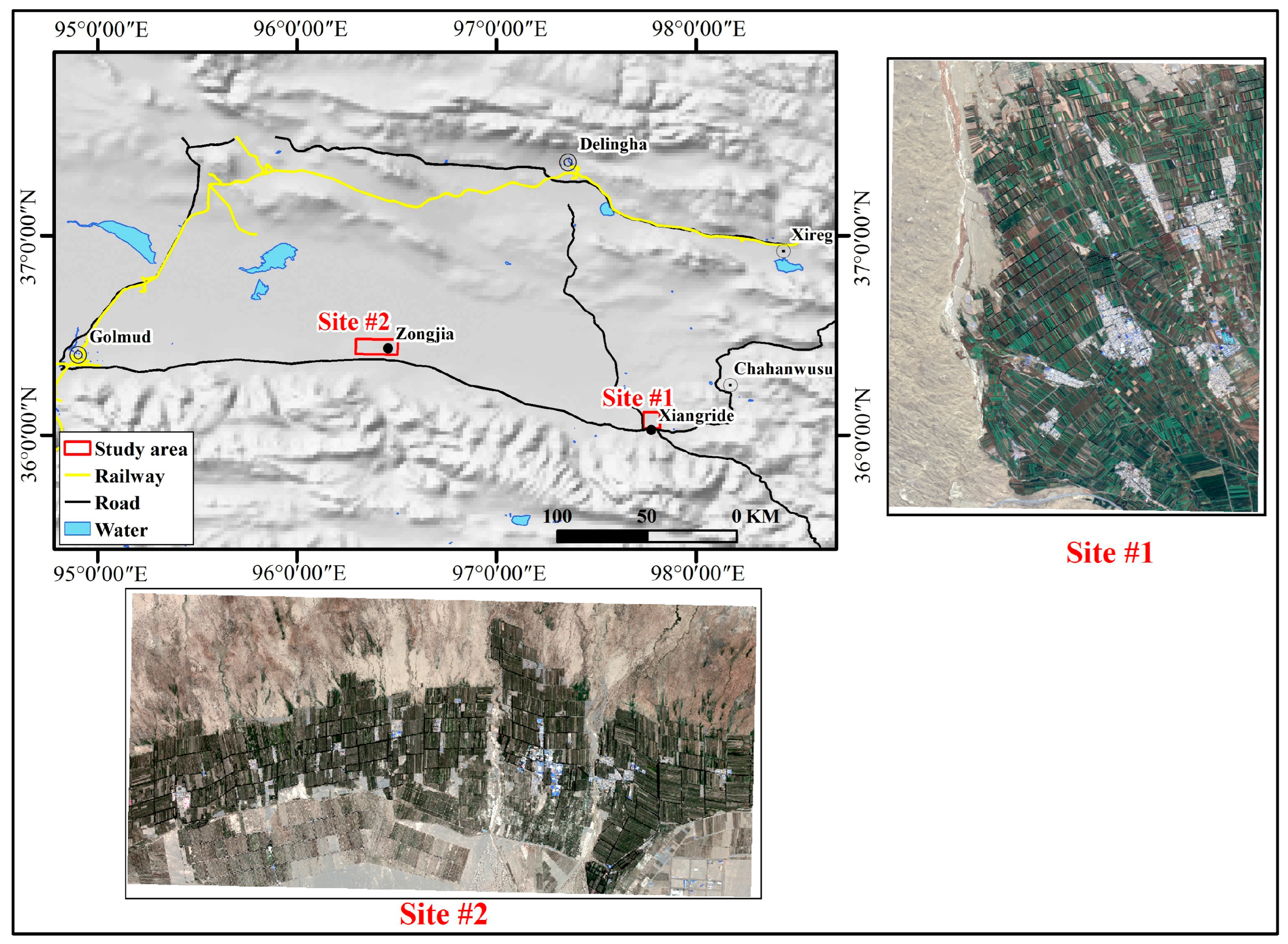
Figure 1. Location of study sites.
Remotesensing 16 01579 g001
Figure 2. Flow chart of crop/vegetation classification with multiple classifiers and multisource remote sensing data.
Remotesensing 16 01579 g002
Figure 3. Field sample distribution of Site #1.
Remotesensing 16 01579 g003
Figure 4. Field sample distribution of Site #2.
Remotesensing 16 01579 g004
Figure 5. Flowchart of OAI-MV.
Remotesensing 16 01579 g005
Figure 6. OA of crop/vegetation classification with single classifier.
Remotesensing 16 01579 g006
Figure 7. OA of crop/vegetation classification for decision fusion.
Remotesensing 16 01579 g007
Figure 8. Crop/vegetation classification results of different decision fusion strategies for Site #1.
Remotesensing 16 01579 g008
Figure 9. Crop/vegetation classification results of different decision fusion strategies for Site #2.
Remotesensing 16 01579 g009
Table 1. Remote sensing data collection of temporal phases and growth stages of crops.
Study AreasSensorsTemporal PhaseGrowing Period of Crops
Site #1Sentinel-112 periods: 13 February 2021, 1 June 202125 June 2021, 1 July 2021, 19 July 2021, 31 July 2021, 24 August 2021, 5 September 2021, 23 September 2021, 29 September 2021, 11 October 2021, 17 October 2021Wheat: Early April~mid-to-late September
Quinoa: April~October
Highland barley: April~October
Rape: April~September
Sentinel-212 periods: 9 February 2021, 4 June 2021, 29 June 2021, 2 July 2021, 22 July 2021, 29 July 2021, 26 August 2021, 7 September 2021, 22 September 2021, 30 September 2021, 12 October 2021, 17 October 2021
GF-622 August 2021
Site #2Sentinel-112 periods: 19 March 2020, 24 April 2020, 30 May 2020, 11 June 2020, 5 July 2020, 29 July 2020, 22 August 2020,3 September 2020, 27 September 2020, 9 October 2020, 21 October 2020, 2 November 2020
Sentinel-212 periods: 19 March 2020, 18 April 2020, 2 June 2020, 17 June 2020, 2 July 2020, 1 August 20201, 26 August 2020, 5 September 2020, 25 September 2020, 30 September 2020, 15 October 2020, 25 October 2020
GF-626 July 2020
Table 2. Comparison of training samples and validation samples for crop classification.
Study AreaCrop TypeTraining SamplesValidation Samples
Site #1wolfberry8 regions/599 pixels7 regions/725 pixels
quinoa14 regions/1135 pixels13 regions/1061 pixels
highland barley5 regions/484 pixels4 regions/416 pixels
wheat18 regions/1541 pixels18 regions/1234 pixels
rape13 regions/687 pixels12 regions/594 pixels
Site #2wolfberry22 regions/1808 pixels21 regions/1685 pixels
quinoa15 regions/692 pixels14 regions/665 pixels
haloxylon11 regions/995 pixels11 regions/955 pixels
wheat14 regions/559 pixels13 regions/620 pixels
poplar20 regions/1262 pixels20 regions/1118 pixels
Table 3. Classification scenarios.
Scenario NotationsFeaturesMethodsScenario NotationsFeaturesMethods
S1SAR (VV + VH)MLS20SAR + GF + VI + BPU-Net
S2SAR (VV + VH)RFS21Results of S1~S4MV
S3SAR (VV + VH)SVMS22Results of S1~S4E-OAI
S4SAR (VV + VH)U-NetS23Results of S1~S4OAI-MV
S5GFMLS24Results of S5~S8MV
S6GFRFS25Results of S5~S8E-OAI
S7GFSVMS26Results of S5~S8OAI-MV
S8GFU-NetS27Results of S9~S12MV
S9VI (NDVI + RVI + SAVI)MLS28Results of S9~S12E-OAI
S10VI (NDVI + RVI + SAVI)RFS29Results of S9~S12OAI-MV
S11VI (NDVI + RVI + SAVI)SVMS30Results of S13~S16MV
S12VI (NDVI + RVI + SAVI)U-NetS31Results of S13~S16E-OAI
S13BP (LAI + Cab + CWC + FAPAR + FVC)MLS32Results of S13~S16OAI-MV
S14BP (LAI + Cab + CWC + FAPAR + FVC)RFS33Results of S17~S20MV
S15BP (LAI + Cab + CWC + FAPAR + FVC)SVMS34Results of S17~S20E-OAI
S16BP (LAI + Cab + CWC + FAPAR + FVC)U-NetS35Results of S17~S20OAI-MV
S17SAR + GF + VI + BPMLS36Results of S1~S20MV
S18SAR + GF + VI + BPRFS37Results of S1~S20E-OAI
S19SAR + GF + VI + BPSVMS38Results of S1~S20OAI-MV
SAR: time series of backscatter coefficients (VV and VH) from Sentinel-1; GF: spectral bands of GF-6; VI: time series of vegetation indices from Sentinel-2; BP: time series of biophysical variables from Sentinel-2.
Table 4. PA, UA, and F1 scores for different crop/vegetation types of classification results with single classifier (Unit: %).
Site #1
WolfberryQuinoaHighland BarleyWheatRape
PAUAF1PAUAF1PAUAF1PAUAF1PAUAF1
S154.3 51.3 52.8 55.5 61.4 58.3 35.7 22.2 27.3 58.3 71.1 64.1 65.5 52.2 58.1
S265.3 71.5 68.2 61.2 63.8 62.5 16.0 37.4 22.4 72.4 67.9 70.1 68.5 59.0 63.4
S356.3 56.7 56.5 61.5 62.5 62.0 28.7 32.3 30.4 67.2 73.0 70.0 73.8 60.9 66.8
S461.1 54.0 57.3 55.5 69.5 61.7 17.4 18.6 18.0 70.0 65.8 67.9 56.8 58.5 57.6
S555.6 58.7 57.1 70.3 65.8 68.0 93.837.7 53.8 54.3 81.0 65.0 88.970.9 78.9
S650.5 71.9 59.3 53.4 66.7 59.3 86.0 38.7 53.3 67.7 71.5 69.5 88.2 64.7 74.6
S748.1 74.1 58.3 71.7 67.8 69.7 87.8 41.1 56.0 66.6 70.2 68.4 88.2 76.8 82.1
S860.2 67.9 63.8 49.7 72.1 58.8 82.4 44.8 58.1 68.9 66.2 67.5 84.7 70.0 76.7
S969.9 83.6 76.1 77.7 73.5 75.5 73.8 64.9 69.1 78.7 80.1 79.4 70.2 62.4 66.1
S1081.1 77.1 79.0 55.3 80.5 65.6 78.9 52.4 63.0 76.5 72.5 74.4 61.1 56.3 58.6
S1185.483.0 84.2 76.0 84.1 79.8 83.6 75.8 79.5 83.781.7 82.772.1 71.2 71.6
S1277.5 77.0 77.2 45.2 78.7 57.4 85.5 38.4 53.0 80.3 69.8 74.7 59.9 67.8 63.6
S1364.0 82.6 72.1 66.5 70.9 68.6 21.4 43.4 28.7 76.0 70.7 73.3 61.3 45.7 52.4
S1480.8 82.0 81.4 57.0 83.6 67.8 72.9 49.8 59.2 79.0 66.5 72.2 41.3 45.6 43.3
S1583.1 86.4 84.778.7 85.381.9 77.8 54.8 64.3 82.6 77.5 80.0 58.9 66.2 62.3
S1680.9 84.0 82.4 70.3 84.0 76.5 76.1 44.6 56.2 77.8 73.5 75.6 61.8 66.3 63.9
S1765.4 82.9 73.1 66.7 76.3 71.2 65.9 65.0 65.4 77.7 72.6 75.1 61.9 49.2 54.8
S1879.7 79.4 79.6 69.7 84.2 76.2 86.9 45.4 59.6 76.2 79.3 77.7 69.3 66.0 67.6
S1980.4 74.8 77.5 70.3 81.9 75.7 91.5 54.0 67.9 80.0 85.282.5 77.8 75.3 76.5
S2082.7 86.684.6 86.580.1 83.282.3 85.784.080.9 80.2 80.5 73.7 77.775.6
Site #2
WolfberryHighland BarleyHaloxylonWheatPoplar
PAUAF1PAUAF1PAUAF1PAUAF1PAUAF1
S170.9 82.3 76.1 12.2 25.5 16.5 76.1 60.5 67.4 69.6 31.1 43.0 86.3 62.1 72.3
S246.9 74.6 57.6 7.5 6.8 7.2 70.6 38.4 49.8 50.5 19.3 27.9 61.4 54.4 57.7
S368.8 81.2 74.5 8.8 16.7 11.5 74.8 42.2 53.9 64.8 36.3 46.5 73.7 73.9 73.8
S489.0 68.3 77.3 5.5 22.7 8.9 46.2 58.0 51.5 4.5 17.2 7.1 10.1 27.8 14.8
S553.3 87.8 66.4 37.6 42.3 39.8 83.650.3 62.8 66.2 36.0 46.7 87.6 88.6 88.1
S670.3 81.7 75.6 46.8 54.6 50.4 69.8 62.3 65.8 52.8 41.0 46.2 90.6 83.3 86.8
S781.3 82.4 81.8 44.0 56.4 49.4 71.7 78.8 75.1 44.6 39.6 41.9 91.8 83.4 87.4
S885.5 88.3 86.8 45.7 64.9 53.6 74.7 79.8 77.2 66.7 44.3 53.3 86.7 94.6 90.5
S988.6 81.2 84.7 72.2 85.2 78.2 52.2 89.6 65.9 89.2 88.2 88.7 94.1 73.0 82.2
S1084.9 87.9 86.4 73.7 86.2 79.4 60.8 89.3 72.3 88.0 87.4 87.7 96.5 88.8 92.5
S1187.0 94.090.4 74.8 93.483.1 78.1 80.8 79.4 94.4 92.4 93.4 95.5 89.0 92.1
S1289.9 93.0 91.5 73.0 84.4 78.3 83.2 84.1 83.6 92.4 92.1 92.3 94.5 95.8 95.2
S1373.5 83.0 78.0 79.4 76.6 78.0 34.6 99.4 51.4 89.2 94.9 92.0 98.7 76.3 86.0
S1488.2 92.6 90.3 76.6 84.0 80.1 59.7 92.6 72.6 91.4 92.7 92.1 99.4 84.1 91.1
S1592.5 95.6 94.0 66.8 87.7 75.8 83.3 88.4 85.8 92.1 86.8 89.4 99.788.6 93.8
S1689.4 91.5 90.4 75.2 89.2 81.6 79.5 85.6 82.5 94.8 87.3 90.9 96.2 90.3 93.2
S1783.7 83.8 83.7 77.9 87.3 82.3 33.0 99.849.6 87.7 95.0 91.2 98.4 69.2 81.2
S1892.7 92.7 92.7 78.4 86.6 82.3 77.2 90.1 83.1 91.9 92.1 92.0 99.3 94.2 96.7
S1993.6 94.093.8 71.6 87.7 78.8 81.6 90.5 85.892.4 91.5 91.9 99.4 89.894.3
S2097.091.5 94.283.589.1 86.275.6 99.1 85.7 96.795.295.992.0 97.294.5
Bold text represents the highest classification accuracy metrics (PA, UA, and F1) for each crop/vegetation type in classification scenarios.
Table 5. PA, UA, and F1 scores for different crop/vegetation types of classification results of decision fusion (Unit: %).
Site #1
WolfberryQuinoaHighland BarleyWheatRape
PAUAF1PAUAF1PAUAF1PAUAF1PAUAF1
S2171.7 61.1 66.0 63.6 69.0 66.2 25.0 26.9 25.9 65.7 71.5 68.5 66.9 61.8 64.2
S2255.3 77.3 64.5 53.3 67.9 59.7 12.3 69.7 20.9 78.2 64.1 70.4 73.4 54.6 62.6
S2363.1 66.8 64.9 63.6 68.0 65.7 13.3 55.3 21.5 74.3 69.6 71.9 71.9 59.6 65.2
S2462.8 72.3 67.2 71.1 68.6 69.8 93.143.9 59.7 63.3 78.1 69.9 88.3 73.7 80.3
S2551.6 81.7 63.2 68.0 73.1 70.5 71.3 75.7 73.5 72.5 67.4 69.9 92.268.1 78.4
S2658.1 78.3 66.7 65.1 71.9 68.3 89.0 50.2 64.2 70.7 73.2 71.9 90.1 70.6 79.2
S2785.2 78.9 81.9 70.4 82.8 76.1 86.1 62.5 72.4 81.2 77.9 79.5 63.8 70.5 67.0
S2883.9 81.8 82.9 74.0 84.0 78.7 82.4 73.9 77.9 84.3 79.9 82.0 69.7 71.3 70.5
S2986.0 83.0 84.5 76.0 84.1 79.8 83.3 77.6 80.4 83.7 81.7 82.7 72.1 71.2 71.6
S3083.4 84.0 83.7 75.6 83.9 79.5 78.1 59.5 67.5 81.6 72.9 77.0 49.5 61.8 54.9
S3186.9 87.3 87.1 83.8 79.4 81.5 61.7 65.8 63.7 83.1 72.8 77.6 44.4 67.7 53.7
S3284.2 85.5 84.8 78.7 84.3 81.4 69.1 68.7 68.9 84.9 72.0 77.9 49.3 67.7 57.1
S3381.6 78.9 80.2 77.4 82.5 79.9 91.5 57.7 70.8 78.8 81.8 80.3 69.9 72.9 71.3
S3482.7 87.8 85.1 83.7 82.0 82.8 82.2 80.4 81.3 84.1 81.1 82.6 71.7 74.6 73.1
S3582.6 86.9 84.7 91.0 79.5 84.8 83.6 85.3 84.4 80.3 82.6 81.4 74.3 78.8 76.5
S3687.1 84.0 85.5 74.6 88.981.1 89.1 73.2 80.4 87.2 82.4 84.7 77.8 78.8 78.3
S3790.8 88.2 89.5 83.5 86.8 85.1 84.6 76.2 80.2 89.2 83.986.471.5 82.6 76.6
S3891.391.291.391.284.8 87.886.7 89.988.389.782.5 85.9 66.7 89.876.5
Site #2
WolfberryHighland BarleyHaloxylonWheatPoplar
PAUAF1PAUAF1PAUAF1PAUAF1PAUAF1
S2180.8 77.8 79.3 7.2 27.8 11.4 71.9 54.1 61.7 57.1 43.1 49.1 72.4 75.2 73.8
S2287.7 72.7 79.5 4.2 58.2 7.9 77.4 57.3 65.8 15.0 67.4 24.5 75.8 70.8 73.2
S2385.7 85.7 85.7 4.2 58.4 7.9 70.1 60.6 65.0 42.8 52.4 47.1 83.2 67.8 74.7
S2483.5 82.3 82.9 42.6 60.2 49.9 73.9 79.3 76.5 56.7 44.5 49.8 85.7 91.0 88.2
S2586.4 82.2 84.2 36.6 74.5 49.1 73.6 81.4 77.3 44.9 41.7 43.2 88.8 83.7 86.1
S2688.5 83.5 85.9 51.9 67.9 58.8 74.8 79.7 77.2 31.6 43.8 36.7 84.6 82.7 83.6
S2792.3 89.4 90.8 76.0 90.5 82.6 71.1 89.3 79.2 92.1 93.3 92.7 95.1 92.2 93.6
S2891.8 92.4 92.1 77.4 88.4 82.5 83.2 85.7 84.4 92.6 92.8 92.7 95.5 92.1 93.8
S2997.2 89.5 93.2 60.2 93.7 73.3 82.9 85.3 84.1 95.6 82.7 88.7 97.5 95.1 96.3
S3092.3 91.4 91.9 77.7 87.3 82.2 61.8 90.9 73.5 92.1 95.2 93.6 99.1 88.1 93.3
S3194.5 90.4 92.4 59.9 90.3 72.0 78.7 86.4 82.4 94.2 85.5 89.6 99.988.3 93.7
S3292.1 92.5 92.3 75.2 87.0 80.7 76.5 90.7 83.0 92.8 92.8 92.8 99.7 87.7 93.3
S3396.0 90.8 93.3 78.988.4 83.4 70.6 94.9 81.0 92.0 95.0 93.4 98.5 94.4 96.4
S3495.8 92.6 94.1 78.8 87.6 83.0 79.3 94.3 86.2 92.5 93.2 92.8 99.0 94.4 96.7
S3595.7 92.5 94.1 75.4 89.4 81.8 82.0 97.0 88.9 96.7 91.9 94.2 99.3 92.4 95.7
S3696.8 95.6 96.2 75.7 97.585.2 88.7 99.5 93.8 99.4 92.5 95.8 97.6 94.7 96.1
S3796.6 95.896.2 76.7 96.9 85.6 90.4 99.694.8 99.693.2 96.3 97.7 94.1 95.9
S3898.695.0 96.879.7 95.3 86.892.498.1 95.299.4 95.697.494.5 99.496.9
Bold text represents the highest classification accuracy metrics (PA, UA, and F1) for each crop/vegetation type in classification scenarios.
Table 6. Comparative analysis of decision fusion accuracy using different OAIs within the OAI strategy (unit: %).
Feature SetSARGFVIBPSAR + GF + BP + VIALL
Site #1Range of OA61.15~64.4364.19~70.8976.78~79.3073.68~76.3477.27~81.4379.86~84.79
OAI of highest OAOAI4OAI5OAI3OAI2OAI2OAI2
OA of OAI163.2364.8778.9774.6380.4682.36
Site #2Range of OA68.97~72.0278.83~80.1082.04~85.5280.93~87.9986.86~92.0788.94~95.07
OAI of highest OAOAI2OAI5OAI6OAI6OAI2OAI2
OA of OAI169.0279.7885.3581.7190.0190.87
Disclaimer/Publisher’s Note: The statements, opinions and data contained in all publications are solely those of the individual author(s) and contributor(s) and not of MDPI and/or the editor(s). MDPI and/or the editor(s) disclaim responsibility for any injury to people or property resulting from any ideas, methods, instructions or products referred to in the content.