GLUENet: An Efficient Network for Remote Sensing Image Dehazing with Gated Linear Units and Efficient Channel Attention

Abstract

Dehazing individual remote sensing (RS) images is an effective approach to enhance the quality of hazy remote sensing imagery. However, current dehazing methods exhibit substantial systemic and computational complexity. Such complexity not only hampers the straightforward analysis and comparison of these methods but also undermines their practical effectiveness on actual data, attributed to the overtraining and overfitting of model parameters. To mitigate these issues, we introduce a novel dehazing network for non-uniformly hazy RS images: GLUENet, designed for both lightweightness and computational efficiency. Our approach commences with the implementation of the classical U-Net, integrated with both local and global residuals, establishing a robust base for the extraction of multi-scale information. Subsequently, we construct basic convolutional blocks using gated linear units and efficient channel attention, incorporating depth-separable convolutional layers to efficiently aggregate spatial information and transform features. Additionally, we introduce a fusion block based on efficient channel attention, facilitating the fusion of information from different stages in both encoding and decoding to enhance the recovery of texture details. GLUENet’s efficacy was evaluated using both synthetic and real remote sensing dehazing datasets, providing a comprehensive assessment of its performance. The experimental results demonstrate that GLUENet’s performance is on par with state-of-the-art (SOTA) methods and surpasses the SOTA methods on our proposed real remote sensing dataset. Our method on the real remote sensing dehazing dataset has an improvement of 0.31 dB for the PSNR metric and 0.13 for the SSIM metric, and the number of parameters and computations of the model are much lower than the optimal method.

1. Introduction

The rapid advancement of earth observation technology has led to the extensive utilization of remote sensing (RS) images in urban management, agricultural inspection, environmental protection, earth sciences, and ocean observation. Nevertheless, the imaging process of optical remote sensing images is frequently affected by atmospheric turbid media, including haze, fog, clouds, and rain. Due to the influence of these atmospheric particles, the imaging light undergoes scattering and attenuation, leading to diminished visibility, reduced contrast, and lower image intensity. Consequently, these factors adversely affect downstream advanced vision tasks, including feature segmentation [1], small target detection [2], and scene classification [3] based on remote sensing images.

Unlike thick clouds that obscure almost all ground-based information, thin clouds and haze are generally translucent, allowing for partial visibility. Whereas the elimination of thick clouds often involves integrating additional data sources to reconstruct missing information via methods such as image fusion, directly dehazing a single remote sensing image stands as a more effective approach for enhancing image quality and broadening applicability. Consequently, the task of removing haze from single remote sensing images, particularly those affected by haze, emerges as a critical and necessary undertaking.

Various dehazing methods have been proposed to address this issue, broadly categorized into two primary categories: a priori-based and learning-based dehazing methods. The a priori-based methods depend on the atmospheric transport equation, which uses physical formulas to model the imaging process of hazy images [4,5,6,7]. However, image dehazing fundamentally represents an inverse problem without a definitive parametric solution, thus requiring the integration of a priori image information and additional constraints for effective resolution. Nevertheless, these hand-crafted features tend to be shallow, rendering these methods unsuitable for complex haze situations. Although a priori-based methods have demonstrated potential in improving dehazing, their effectiveness largely depends on the alignment with their underlying assumptions, rendering them more appropriate for particular scenarios that conform to these assumptions. For instance, despite the simplicity and effectiveness of dark-channel dehazing [4], significant color distortions persist in the dehazing results of remote sensing images.

Learning-based approaches [8,9,10,11] train parametric end-to-end dehazing models using pairs of hazy images and corresponding clear images, employing the model’s forward process to establish a mapping from hazy images to clear images. Significant advancements in remote sensing image dehazing have been made through learning-based methods, such as convolutional neural networks (CNNs), which leverage large-scale remote sensing image datasets for training, eliminating the need for manual feature extraction or intricate a priori model design. Learning-based techniques are particularly proficient in managing complex scenes, such as urban landscapes, mountainous terrains, and watersheds, where diverse lighting conditions and varied texture structures are present.

However, with the development of deep learning methods and the improvement of hardware level, the models of today tend to have a huge number of parameters and a high computational demand, which is too inefficient to process the massive and large-scale remote sensing data. In the previous remote sensing dehazing methods, the complexity and computational burden of the model are seldom considered, which affects its practical application ability. In order to satisfy the practical needs, the goal of this study is to propose a simple and effective dehazing network for remote sensing images. We will construct our data-driven remote sensing dehazing method based on both training data and network models.

Initially, we examine the domain gap between remotely sensed images and natural images. In comparison to general natural images, remote sensing images encompass a broader imaging perspective, more abundant features, and more complex atmospheric conditions. Concerning the dehazing task, the spatial distribution of haze in remote sensing images and its distribution across different wavebands are uneven. The uneven spatial distribution indicates that haze is not uniformly distributed across the entire image (including regions of clean pixels), and the thickness and particle size of the haze can vary at different coordinate points, leading to variability in the imaging results. The uneven distribution of wavelengths refers to the distinct penetration capabilities of electromagnetic waves of different wavelengths to atmospheric particles such as clouds and haze. Generally, the longer the wavelength, the greater its penetration capability through atmospheric particles, resulting in imaging images of different wavelengths being affected differently by various particles in clouds and haze. Most previous remote sensing image dehazing datasets are based on synthetic dehazing images generated from real remote sensing images. To enhance the network’s generalization, we construct real hazy–clear image pairs for training, utilizing the characteristic ten-day revisits to the ground by remote sensing satellites.

To address the aforementioned challenges, remote sensing image dehazing fundamentally involves an image recovery process in more complex scenarios. Drawing inspiration from methods in image restoration, some researchers employ a U-Net [12]-style network architecture to achieve state-of-the-art (SOTA) results [13,14]. Additionally, The authors in [13] emphasize that increasing system complexity is not the sole method to enhance performance: a simple baseline can also achieve SOTA performance. Following this strategy to construct our network structure architecture, we initially utilize the classical U-Net, along with local residuals and global residuals as our base architecture, to extract multi-scale information. Subsequently, we employ a depth-wise separable convolutional layer [15] for the aggregation of spatial information and the efficient transformation of features. Moreover, the task of extracting global information is delegated to an attention-guided fusion module, which dynamically merges feature maps from various path channels. Correspondingly, two key modules are proposed: a residual block with a gating mechanism called a GLUE block and a fusion module with an efficient channel attention (ECA) mechanism [16] called ECA Fusion. We assess the performance of our network, GLUENet, on both synthetic and real remote sensing dehazing datasets. As shown in Figure 1, for the first row of the synthetic hazy image, the traditional dark-channel dehazing method (DCP) [4], CNN-based dehazing network (AOD-Net) [8], vision transformer-based dehazing network (DehazeFormer) [11], and our method all exhibit commendable performance. These methods effectively counteract the uneven haze present in the hazy image. However, the dehazing results obtained by the two comparative methods (AOD-Net and DehazeFormer) are unsatisfactory when addressing the real hazy image in the second row of Figure 1. AOD-Net reveals several traces of residual haze, while DehazeFormer is unable to naturally restore features obscured by the real haze. The experimental results demonstrate that GLUENet achieves performance comparable to the related Transformer method with significantly lower overhead.

The main contributions of this paper are as follows:

• We developed GLUENet, an encoder–decoder remote sensing image dehazing network, with less model complexity and computational effort, achieving superior results.
• We construct basic convolutional blocks (GLUE blocks) using gated linear units and efficient channel attention while using depth-separable convolutional layers to aggregate spatial information and efficiently transform features.
• We proposed an attention-guided fusion block based on efficient channel attention (ECA Fusion), integrating information from different stages in both encoding and decoding to enhance the dehazing effect.
• We created a real remote sensing image haze-clear dataset using Sentinel-2 satellite remote sensing images.

2. Related Work

2.1. Image Dehaze

According to the results [17,18] of previous studies by relevant atmospheric optics researchers, it is known that the traditional physical model of haze imaging is the following calculation formula:

$$I(x)=t(x)J(x)+(1-t(x))A$$

(1)

where $A$ represents the global atmospheric light, which is typically constant, $t\left(x\right)$ represents the transmission map, whose value varies with pixel, and $J\left(x\right)$ represents the pixel value of a clear image. The transmission map in situations with inhomogeneous haze can also be represented by the equation that follows:

$$t(x)=e^{-\beta (x)d}$$

(2)

where $d$ is the scene depth and $\beta$ represents the scattering coefficient of the atmosphere.

For remote sensing non-uniform haze, due to the inhomogeneity of the spatial distribution of the haze, the previous simple physical formulas cannot accurately model the real situation of remote sensing haze. According to the theory of Nayar et al. [17], the variable $d$ represents the thickness of the medium that scatters light. When the path from the scene to the observer is permeated with uniform haze, the parameter $d$ can be replaced by the depth of field. In remote sensing imaging, $d$ becomes a length value, denoted as $d\left(x\right)$, that varies according to the pixel. Additionally, the transmission map, denoted as $t\left(x\right)$, is related to wavelength and haze conditions. Therefore, the $t\left(x\right)$ of a remote sensing image emerges as a complex function, dependent on both spatial location and wavelength. According to the theory of Song et al. [11], the transmission map can be expressed as follows:

$$t(x)=e^{-\beta (\lambda ,y(x))d(x)}$$

(3)

where $\lambda$ is the center wavelength of the RS image band, and the exponent $\gamma \left(x\right)$ is indicative of the haze conditions specific to each region.

Based on the above and other physical models, numerous studies on dehazing natural images and remote sensing images have originated from this foundation. The majority of the initial methodologies were heavily reliant on a priori knowledge. He et al. [4] proposed a method based on the Dark Channel Prior (DCP), grounded in the critical observation that haze-free outdoor images frequently exhibit areas where pixels demonstrate notably low intensities in at least one color channel, thereby assisting in the estimation of the transmittance map. In contrast, the Color Attenuation Prior (CAP) method [5] establishes a linear relationship between depth, luminance, and saturation from the HSV color model. An automatic and empirical method for identifying and eliminating non-uniform haze in medium- to high-resolution satellite optical multispectral pictures is presented by Makarau et al. [7]. In order to facilitate spectrally consistent haze removal for RS multispectral data, the dark matter subtraction approach was further extended to compute haze thickness maps.

In recent years, with the emergence of deep learning techniques and the surge of big data, CNNs have found successful applications in the field of remote sensing. Cai et al. [19] employ DehazeNet, incorporating feature extraction and nonlinear regression layers to recover images. Subsequently, by redefining the equations of the atmospheric scattering model, AOD-Net [8] adopts a novel end-to-end dehazing design to directly generate clear images with a lightweight CNN. FFANet [10] introduces an innovative Feature Attention (FA) module that combines Channel Attention and Pixel Attention mechanisms, enhancing the network’s representational capability and significantly outperforming previous dehazing methods. DehazeFormer [11], built upon the popular Swin Transformer [20], refines its modules to suit image dehazing and introduces RSHaze, a large-scale remote sensing synthetic dataset closer to real remote sensing situations. To map haze images to haze-free images, RSDehazeNet [21] also uses a Global Residual Learning (GRL) structure and a channel attention technique. In order to overcome this difficulty, FCTF-Net [9] created a two-stage dehazing neural network, which is refined after the coarse step. The structure is straightforward yet efficient: an encoder–decoder architecture is used in the first stage of picture dehazing to extract multi-scale features, which enables the second stage of dehazing to refine the output of the first stage. Chen et al. [22] introduced a non-uniform dehaze network tailored for visible remote sensing images with non-uniform haze. Drawing inspiration from the well-known gather-excite attention module, they propose the non-uniform excitation (NE) module. This NE module is recursively incorporated into the multi-scale framework, enhancing learning efficiency while reducing network parameters. A network (M2SCN) was developed by Li et al. [23] to handle non-uniform scenarios in RS haze. The multi-model joint estimation (M2JE) module enhances the model’s generalization ability by approaching the dehazing procedure as a multi-model integration problem. Additionally, the network collects intermediate characteristics and uses the self-correcting (SC) module to gradually repair defects in those characteristics. For the purpose of dehazing aerial images, Kulkarni et al. [24] suggested a novel deformable multi-head attention mechanism with a spatial attention offset extraction solution. For visible light Remote Sensing Imagery (RSI), He et al. [25] presented a unique haze removal algorithm known as HALP based on heterogeneous atmospheric light prior and side window filtering. An algorithm for dehazing visible light remote sensing images, called SRD, was presented by He et al. [26]. Initially, superpixels are used to partition the remote sensing hazy image into content-aware patches, and a technique is developed to estimate the local atmospheric light and transmission within each superpixel.

In addition to general data-driven approaches, there is also work on dehazing using weak supervision. Zhao et al. [27] proposed a two-stage weakly supervised dehazing framework combining dark channel and CycleGAN [28]. In the first stage, the dark channel is used to prioritize the restoration of visibility. Then, in the second stage, the initial dehazing results from the first stage are refined through the adversarial learning of unpaired hazy and clear images. In addition, the contrast learning approach has been applied to the field of image dehazing; Chen et al. [29] introduced contrast learning into the CycleGAN framework and achieved an encouraging performance. Although weakly supervised learning achieves good performance, there is still a gap between its performance and that of models trained on paired datasets.

None of the methods mentioned above are completely independent of the reliance on the atmospheric transport equation. A priori-based methods inherently require the utilization of the atmospheric transport equation to compute clear images. On the contrary, learning-based methods primarily utilize training datasets consisting of hazy images synthesized by applying atmospheric transport equations to clean images. This limitation stems from the degree to which these physical equations correspond with real-world scenarios, consequently impeding the generalizability of these methods.

2.2. Gated Linear Units

Gated linear units (GLUs) can be interpreted by generating two linear transformation layers by elements, one of which is activated with nonlinearity. GLU has found extensive applications in both natural language processing [30,31] and computer vision [32], demonstrating its effectiveness in the realm of image restoration [13,14]. The mathematical formulation of gated linear units is expressed as follows:

$$\mathrm{GLU}(x,f,g,\sigma )=f(x)\odot \sigma (g(x))$$

(4)

where $x$ denotes the input feature map, $f\left(x\right)$ and $g\left(x\right)$ are linear transformers, $\sigma$ is the nonlinear activation function, and ⊙ indicates element-wise multiplication.

Similarly, when we observe the formulas for the activation function and pixel attention, the GELU [33] activation function and channel attention are used as examples. An approximate implementation of GELU can be represented as follows:

$$\mathrm{GELU}(x)=x\mathsf{\Phi }(x)=0.5x(1+tanh[\sqrt{2/\pi }(x+0.044715x^3)])$$

(5)

where Φ indicates the cumulative distribution function of the standard normal distribution. The channel attention [34] is calculated by the following formula:

$$\mathrm{CA}(x)=x\ast \sigma (W_{2}max(0,W_{1}pool(x)))$$

(6)

where $pool$ denotes the global average pooling procedure, which aggregates the spatial data into channels, and $x$ stands for the feature map. The nonlinear activation function, or Sigmoid, is represented by $\sigma$. ReLU is performed in the connection between $W_1$ and $W_2$, two fully connected layers. Lastly, the symbol ∗ signifies a channel-wise product operation. Building upon channel attention, Chen et al. [13] took a further step and introduced simplified channel attention, which is formulated as follows:

$$\mathrm{SCA}(x)=x\ast Wpool(x)$$

(7)

Upon examining Equations (4) and (5), it becomes apparent that when $f\left(x\right)$ and $g$(x) are identity functions, Φ can also be treated as a nonlinear activation function, thereby categorizing GELU as a gated linear unit under certain conditions. Further, by scrutinizing Equations (4) and (7), it is evident that by employing the same simple substitution of functions in GLU, the simplified channel attention can be considered a special case of GLU. Drawing a parallel, we hypothesize from another perspective that GLU might be seen as a generalization of channel attention for activation functions, potentially serving as a substitute for both nonlinear activation functions and pixel attention.

Numerous SOTA research works in image restoration have demonstrated that the addition of gated linear units to the baseline network can enhance network performance. Zamir et al. [14] introduced a gating mechanism to a regular feed-forward network (FN), involving an element-wise multiplication of two parallel paths of the linear transformation layer, with one path nonlinearly activated by GELU. The FN is further augmented by integrating gated deep convolution, leading to significant performance improvements. A simple variation in gated linear units has been demonstrated with NAFNet [13], in which the feature map is divided into two sections along the channel dimension and then multiplied.

This variant replaces the nonlinear activation function in the network, resulting in performance enhancement for image denoising and deblurring tasks. The tasks of remote sensing image dehazing and image restoration are underpinned by the same fundamental network model, with both endeavors focused on learning the mapping from a degraded image to its real counterpart. The degradation process involved in the cloudy imaging of remote sensing images is typically more complex. However, the gated linear unit, when applied through multiplication with the feature map via an alternate branch, adeptly integrates the spatial distribution of haze and band difference information into the feature extraction phase. This approach, in turn, leads to a further enhancement in the performance of real remote sensing image dehazing in comparison to the baseline model.

3. Proposed Method

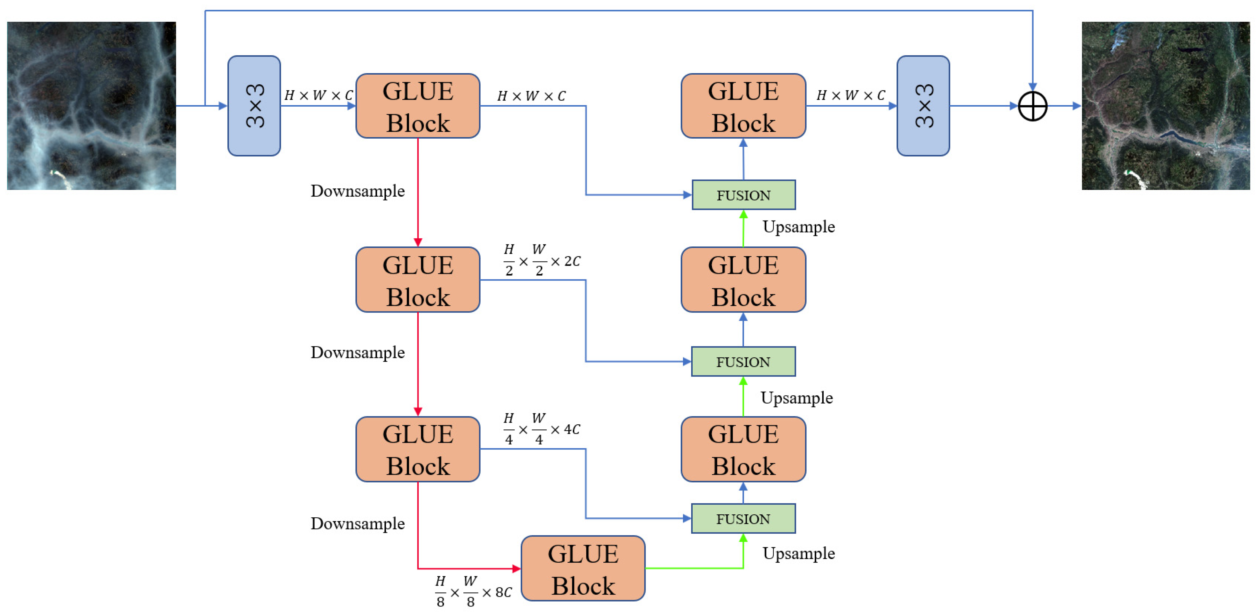
3.1. Network Architecture

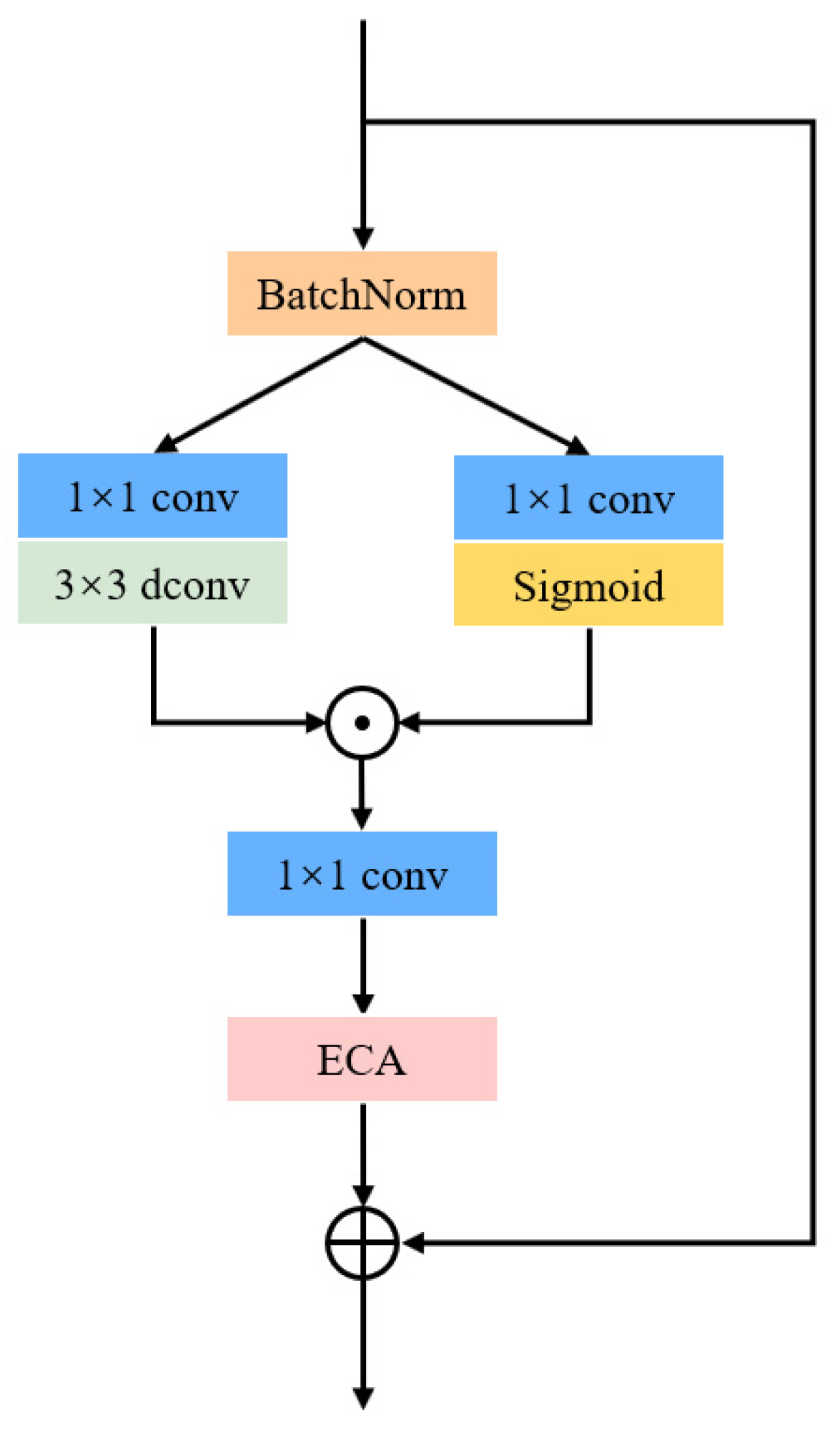
Figure 2 illustrates the overall architecture of our GLUENet network. Our model constitutes a 7-stage variant of U-Net, with each stage integrating a series of our innovatively proposed GLUE blocks. Additionally, our approach diverges from U-Net’s conventional strategy, which employs cascading post-convolutional layers to amalgamate jump connections and the primary path. Instead, we utilize the ECA Fusion module to dynamically fuse feature maps from diverse paths.

GLUENet first uses convolution to create a low-level feature $F_0\in {ℝ}^{H\times W\times C}$ embedding from a hazy image $I\in {ℝ}^{H\times W\times 3}$, where $H\times W$ stands for spatial dimensions and $C$ for the number of channels. These shallow characteristics are then converted into deep features using a three-level symmetric encoder–decoder. The encoder–decoder uses numerous GLUE blocks in each level. The encoder increases the channel capacity and gradually shrinks the spatial size, starting with high-resolution inputs. The high-resolution representation is methodically restored by the decoder using low-resolution latent characteristics as input. We use a conventional convolutional layer approach for feature downsampling, setting the stride value to 2 and doubling the number of output channels in comparison to the number of input channels. We employ the 1 × 1 Conv + PixelShuffle method to perform upsampling. The ECA Fusion module connects the encoder and decoder features to speed up the recovery process and preserve more fine structure and texture details in the recovered image. These design choices lead to observable quality gains, as the experimental section shows. Finally, a 3 × 3 convolutional layer is used to transform the feature dimension from $C$ to 3 to generate the residual image $R\in {ℝ}^{H\times W\times 3}$. And, it is added to the original image to obtain the recovered remote sensing image: $\widehat{I}=I+R$.

The process of training involves reducing the pixel difference between the associated ground truth $GT$ and the anticipated haze-free image $\widehat{I}$. To make training easier, we use the L1 loss function (i.e., mean absolute error) in our implementation.

$${ℒ}_{L1}=\Vert \widehat{I}-GT{\Vert }_1$$

(8)

3.2. GLUE Block

Based on previous dehazing networks, the base modules can be broadly categorized into two types: one is a CNN block that incorporates channel attention and spatial attention, and the other is a transformer block that employs self-attention. Dehazing in RS images is associated with the perception of haze, implying that the network should encode the global information of the haze distribution, necessitating a larger effective receptive field. Expanding the receptive field by enlarging the window in conventional CNNs and transformer blocks leads to a quadratic increase in parameters and computation. However, studies have demonstrated that simply replacing the activation function with GLU in the baseline enhances the performance of image recovery, with GLU incurring less computational overhead while efficiently capturing global information from features. The foundational block of our dehazing network primarily relies on GLU. We use this as a basis to build our GLUE block, details of which can be seen in Figure 3. Let x represent the feature map, initially normalized using BatchNorm as $\widehat{x}=BatchNorm\left(x\right)$. Although some methods suggest that using LayerNorm can enhance dehazing performance, we observed no performance improvement in our experiments. Instead, BatchNorm offers faster inference and aligns better with the characteristics of our lightweight network.

$$\begin{array}{c}{x}_1=\mathrm{Sigmoid}({\mathrm{PWConv}}_1(\widehat{x}))\\ x_2=\mathrm{DWConv}({\mathrm{PWConv}}_2(\widehat{x}))\end{array}$$

(9)

where PWConv represents the point-wise convolutional layer, i.e., 1 × 1conv, and DWConv represents the depth-wise convolutional layer. We subsequently employ $x_1$ as the gating signal for $x_2$ and project it using another 1 × 1 Conv, which can be formulated as follows:

$$x_3={\mathrm{PWConv}}_3(x_1\cdot x_2)$$

(10)

Lastly, $x_3$ is calculated for its efficient channel attention. The computed attention channel weights and feature $x_3$ undergo a dot multiplication, and the output is subsequently added to the constant shortcut x, which can be formulated as follows:

$$y=x+x_3\cdot \mathrm{ECA}(x_3)$$

(11)

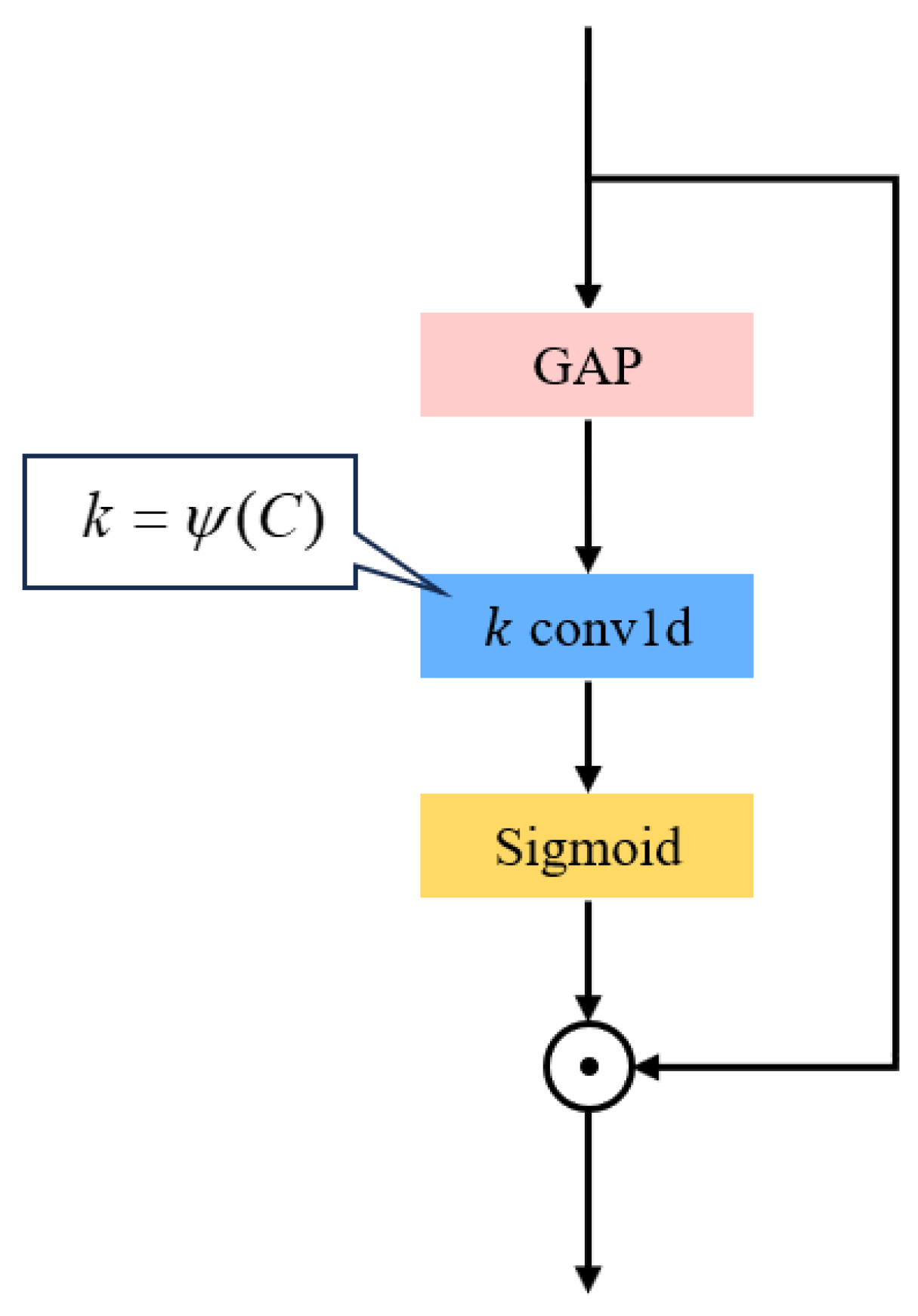
3.3. Efficient Channel Attention

Since the proposal of attention mechanisms, they have demonstrated a significant improvement in model performance in both natural language processing and computer vision domains. In the vision domain alone, applications include channel attention [34], CBAM [35], dual attention [36], and vision transformer [37], with numerous attention modules present in previous image dehazing networks. While the attention mechanism has achieved remarkable success in many tasks, it has some potential drawbacks. For instance, using the attention mechanism typically requires more computational resources because the model needs to compute the weights as each input is processed, potentially leading to higher computational costs for training and inference. To align with the characteristics of lightweight networks, we opt for efficient channel attention [16] as our method for global information feature extraction.

Figure 4 shows the efficient channel attention (ECA) module. ECA creates channel weights by performing a quick one-dimensional convolution of size $k$ with the aggregated data acquired through global average pooling. The value of k is adaptively determined by mapping the channel dimension $C$. With ECA, local cross-channel interactions are captured efficiently since every channel and its $k$ close neighbors are considered. It is shown that this method guarantees both efficacy and efficiency when compared to traditional channel attention strategies. The coverage of local cross-channel interactions, or the number of neighbors participating in a channel’s attentional prediction, is shown by the kernel size $k$ in this instance. We use an adaptive approach to find $k$, where the coverage of the interaction (i.e., kernel size $k$) is proportional to the channel dimension. The formula is as follows:

$$k=\psi (C)={\left|\frac{lo{g}_2(C)}{\gamma }+\frac{b}{\gamma }\right|}_{odd}$$

(12)

where ${\left|t\right|}_{odd}$ denotes the closest odd number to $t$. In this paper, we set $\gamma$ and $b$ to 2 and 1 in all experiments, respectively. It is evident that by mapping $\psi$, the high-dimensional channels exhibit longer-range interactions, while the low-dimensional channels display shorter-range interactions through the application of a nonlinear mapping. We added ECA to our base GLU block to improve the dehazing performance of the model, which was verified in subsequent ablation experiments.

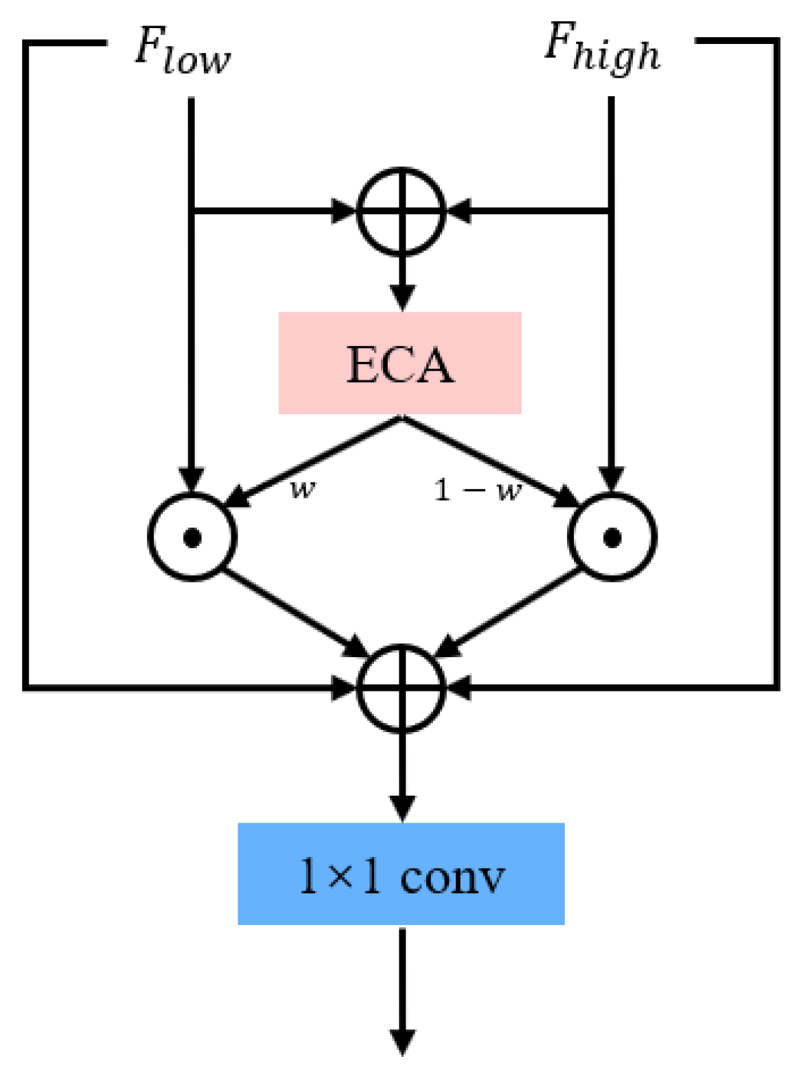
3.4. Attention-Guided Fusion

We acknowledge that an efficient approach for dehazing and other low-level visual tasks is the combination of characteristics from the encoder and the decoder. Although low-level elements (such as edges and contours) are important for retrieving images free of haze, their influence rapidly decreases as they move through multiple intermediate levels. By enhancing the information flow from shallow to deep layers, feature fusion makes gradient backpropagation and feature retention easier. The simplest fusion method involves element-wise addition, commonly used in previous approaches [13,38]. However, the aforementioned fusion scheme encounters receptive field mismatch. The information encoded within shallow features substantially diverges from that in deep features, owing to their distinctly different receptive fields. Individual pixels in deep features correspond to pixel regions in shallow features. Basic addition, concatenation, or blending operations cannot address the mismatch issue before fusion.

In order to tackle this problem, we furthermore present an ECA-based hybrid technique that uses learned spatial weights to alter the features in order to dynamically combine the low-level features in the encoder section with the corresponding high-level features. Details of the suggested ECA-based hybrid fusion scheme are shown in Figure 5. It is important that we decide to compute channel weights for feature change using ECA. The low-level attributes from the encoder section are combined with the corresponding high-level features that are sent into the ECA for weight calculation using weighted summation. We create skip connections to include input information, which alleviates the gradient vanishing issue and speeds up the learning process. Projecting the fused features via a 1 × 1 convolutional layer yields the final features.

$$F_{fusion}=Con{v}_{1\times 1}(W\cdot F_{low}+(1-W)\cdot F_{high}+F_{low}+F_{high})$$

(13)

4. Experimental Results

4.1. Dataset Generation

Remote sensing haze imaging in the real world is intricate and diverse, and most of the previous dehazing studies have created datasets by artificially introducing haze to clear remote sensing imagery. Although synthetic datasets may provide benefits in certain scenarios, they also possess inherent limitations. Synthetic data, being generated based on assumptions and rules, may have a distribution distinct from real data. Real-world data can encompass a range of situations, contexts, and variations, along with diverse noise and uncertainties that are challenging to accurately model with synthetic data. Consequently, models trained on synthetic datasets often exhibit reduced effectiveness when applied to real haze remote sensing images, impacting the method’s generalizability.

Inspired by prior research [39,40], we recognized the effectiveness of constructing a dataset by capturing brief satellite revisits to the Earth’s surface. Sentinel-2A [41], equipped with a multispectral imager (MSI), operates as a high-resolution multispectral imaging satellite. The wavelength range of Sentinel-2A satellite images spans from 0.443 to 2.190 $\mathsf{\mu }\mathrm{m}$, with a revisit time to the surface of ten days. Leveraging the characteristics of Sentinel-2 data, we randomly selected remote sensing images from various locations worldwide and across different seasons. We meticulously selected pairs of clear and hazy remote sensing images, captured ten days apart, to construct an authentic remote sensing haze removal dataset, with the objective of enhancing both the performance and the generalizability of the model.

This study utilized haze-covered and corresponding clear images from the Sentinel-2A satellite for training and testing all methods. To comprehensively assess dehaze effectiveness across extensive areas and diverse land cover types, the training and testing regions are uniformly distributed globally, as illustrated in Figure 6. These regions encompass three primary land cover types: urban, vegetated, and bare ground. We manually selected 36 pairs of Sentinel-2A Level-1C products, with acquisition dates spanning from 2015 to 2019, representing all seasons. We do not carry out anything extra for imaging changes within 10 days. We believe that the effect of small feature variations that may arise from the ten days is extremely limited and that a moderate amount of noise increases the generalizability of our method. Leveraging the GDAL library, we initially extracted the visible RGB bands, cropped them into 512 × 512 image blocks, and then filtered out blocks with missing values. The remaining blocks were saved as single TIFF images with a size of 512 × 512 pixels. Subsequently, the training and test sets were randomly divided in a 9:1 ratio, resulting in 13,205 pairs for the training set and 1468 pairs for the test set.

Our dataset, RRSH (Real Remote Sensing Haze), is generated from authentic pairs of remote sensing images, uniformly distributed worldwide, encompassing various land cover types and seasonal variations. In contrast to previous synthetic datasets, the clouds and haze in our dataset exhibit greater randomness and heterogeneity, providing a more realistic depiction of cloud scenarios in remote sensing images.

4.2. Experimental Settings

4.2.1. Datasets

Our experiments are primarily conducted on the RSHaze dataset and our RRSH dataset. The primary synthesis process of the RSHaze dataset involves using clear Landsat remotely sensed images to acquire haze-free image blocks from various terrains. Subsequently, cloudy remote sensing images are chosen, and their cirrus channels are utilized to generate transmission maps, resulting in cirrus channel blocks with distributions resembling natural haze. Haze density is regulated by additional parameters to generate nine synthetic haze images, each with three different haze densities, for every haze-free image. RSHaze stands out as the largest and most realistic synthetic dataset currently available, comprising 51,300 paired images for training and 2700 paired images for testing. Additionally, RRSH is our haze-clear dataset based on real remote sensing images. The synthesis process avoids any physical simulation modeling formulas and faithfully represents the situation, background, and noise of remote sensing haze image imaging. The resolution of all sample images in the RSHaze and RRSH datasets is uniform at 512 × 512.

4.2.2. Implementation Details

In all experiments, we employ the following training parameters in all of our trials. We employ a four-level encoder–decoder in our GLUENet. The number of GLUE blocks is [2, 2, 2, 4] from level 1 to level 4, and the number of channels per stage is [32, 64, 128, 256]. Using the Adam [42] optimizer (β1 = 0.9, β2 = 0.999), we train the model on the RSHaze dataset for a total of 200,000 iterations. Initially, we set the learning rate at 1 × 10⁻³, and then gradually reduce it to 1e-6 using a cosine annealing scheme [43]. For every GPU, a batch size of 16 is assigned, and the training patch size is 256 × 256. We established a lower limit of 100,000 iterations for the RRSH dataset while maintaining all other configurations. We use PyTorch (version 1.11.0) to implement the suggested network on a system that has eight NVIDIA TITAN XP GPUs.

4.2.3. Evaluation Metric and Benchmark Methods

Drawing on the evaluation indices commonly used in other research within the field of image dehazing, we have selected PSNR (Peak Signal-to-Noise Ratio), SSIM (Structural Similarity Index Measure) [44], MS-SSIM (Multi-Scale Structural Similarity) [45], and FSIM (Feature Similarity Index) [46] as the evaluation metrics for assessing the remote sensing dehazing capability in this study. Higher values of these evaluation metrics indicate the superior remote sensing dehazing performance of the method. Additionally, we have chosen the number of parameters (#Param), MACs (Multiply-Accumulate Operations), and latency as metrics to gauge the model’s overhead, with the size of MACs calculated based on an input image size of 256 × 256. The inference latency is measured as the time it takes to infer a 3 × 256 × 256 image on an NVIDIA 4090 GPU, and we take the average of it three times as an evaluation metric. A smaller number of parameters and MACs signifies a reduced overhead required by the model, which also suggests a faster inference capability. The PSNR is calculated using the following formula:

$$\mathrm{PSNR}=10lo{g}_{10}\left(\frac{ma{x}^2}{MSE}\right)$$

(14)

Here, $max$ denotes the signal peak, which corresponds to the maximum pixel value within the RGB channels of the remote sensing image. $MSE$ represents the mean square error between the two images being compared.

The SSIM evaluates three fundamental aspects of an image: luminance, contrast, and structure. SSIM is capable of quantifying the extent of distortion within an image, as well as the degree of similarity between two images. Consequently, it aligns more closely with the intuitive visual perception of the human eye. SSIM is defined as follows:

$$\mathrm{SSIM}(x,y)=\frac{\left(2u_x{u}_y+C_1\right)\left(2{\sigma }_{xy}+C_2\right)}{\left(u_x^2+u_y^2+C_1\right)\left({\sigma }_x^2+{\sigma }_y^2+C_2\right)}$$

(15)

where $u_x$ and $u_y$ represent the mean values of $x$ and $y$, respectively; ${\sigma }_{xy}$ denotes the covariance of x and y; ${\sigma }_x$ is the variance of $x$; ${\sigma }_y$ is the variance of $y$; and $C_1$ and $C_2$ are constants employed to ensure stability in the calculation. To enhance SSIM’s ability to depict an image’s local and global structure, MS-SSIM incorporates multi-scale analysis. The final MS-SSIM value is determined by first decomposing the image, calculating the SSIM values at each scale independently, and then combining these values.

FSIM is a similarity metric based on the local features of an image. Its calculation formula is as follows:

$$\mathrm{FSIM}(x,y)=\frac{{\displaystyle \sum _w}(f_x(w)\cdot f_y(w))}{\sqrt{{\displaystyle \sum _w}{f}_x^2(w)\cdot \sum _w{f}_y^2(w)}}$$

(16)

where $f_x\left(w\right)$ and $f_y\left(w\right)$ are the feature vectors of the images $x$ and $y$, respectively, over a localized window $w$; $w$ is the position of the window, usually a local region in the image.

Our dehazing network is compared to four cutting-edge techniques: AOD-Net [8], GCANet [47], FCTF-Net [9], and DehazeFormer [11], as well as one conventional method, DCP [4]. For the deep learning methods, we use the authors’ official code to retrain and obtain test results. And, we choose the higher of our reproduced results and the results in the authors’ original text as our benchmark for a fair comparison.

4.3. Quantitative Evaluations

4.3.1. Quantitative Evaluations on RSHaze Dataset

Table 1. Evaluation metrics and overhead of contrasting methods on the RSHaze dataset. For comparing methods, we use bold and italics to mark the best method.

Methods	RSHaze				Overhead
	PSNR	SSIM	FSIM	MS-SSIM	#Param (M)	MACs (G)	Latency (ms)
DCP	17.81	0.729	0.808	0.702	-	-	-
AOD-Net	26.67	0.858	0.888	0.840	0.002	0.115	14.67
GCANet	34.05	0.952	0.965	0.962	0.702	18.47	127.98
FCFT-Net	36.33	0.963	0.970	0.969	0.159	10	119.60
DehazeFormer-B	39.87	0.971	0.979	0.980	2.514	25.79	714.02
GLUENet (ours)	38.98	0.973	0.977	0.978	1.44	4.62	123.13

presents the average evaluation metrics of our method and various comparative methods on the RSHaze test set on the left, while on the right it illustrates the computational costs and latency required for the inference of a 3 × 256 × 256 image with different methods. It can be observed from the table that the PSNR of the DCP method on the RSHaze dataset is merely 17.81 dB. This indicates that traditional a priori-based dehazing methods encounter significant challenges when applied in remote sensing applications, resulting in relatively inferior performance. Conversely, AOD-Net exhibits markedly superior evaluation metrics on remote sensing datasets compared to DCP, showcasing the substantial potential of data-driven methodologies in remote sensing image dehazing. On the RSHaze dataset, GCANet, FCTF-Net, DehazeFormer, and GLUENet achieve higher PSNR values, all exceeding 30 dB, indicating their stronger dehazing capabilities. When comparing metrics such as SSIM and its related variants, it is evident that the latter four deep learning methods have achieved significantly superior performances, with slight differences between their metrics. It is worth noting that our method, GLUENet, has a slightly higher SSIM value than DehazeFormer. Furthermore, contrasting the computational costs required for the inference of a single image by different methods reveals a trend: the improvement in model performance is accompanied by an increase in computational costs. However, our method achieves performance comparable to SOTA methods with significantly lower computational costs when applied to synthetic remote sensing datasets.

4.3.2. Quantitative Evaluations on RRSH Dataset

Table 2. The evaluation metrics and overhead of contrasting methods on the RRSH dataset. For comparing methods, we use bold and italics to mark the best method.

Methods	RRSH				Overhead
	PSNR	SSIM	FSIM	MS-SSIM	#Param (M)	MACs (G)	Latency (ms)
DCP	18.77	0.723	0.862	0.820	-	-	-
AOD-Net	27.11	0.853	0.886	0.863	0.002	0.115	14.67
GCANet	27.61	0.888	0.913	0.901	0.702	18.47	127.98
FCFT-Net	32.31	0.925	0.927	0.920	0.159	10	119.60
DehazeFormer-B	33.26	0.925	0.935	0.931	2.514	25.79	714.02
GLUENet(ours)	33.57	0.938	0.938	0.934	1.44	4.62	123.13

shows the average evaluation metrics and overhead of our method and various comparative methods on the RRSH test set. Unlike on the synthetic dataset, the metrics vary more from method to method. This proves that real remote sensing datasets have greater variability. On the RRSH dataset, our method outperforms DehazeFormer, achieving the highest in all evaluation metrics. We attribute this, in part, to the limitation of the graphics card’s memory size, preventing DehazeFormer from using a larger batch size per graphics card during training, leading to a performance loss. Additionally, we employ #Param., MACs, and latency as the primary metrics to evaluate computational efficiency. Previous dehazing methods were characterized by relatively small parameter sizes, but this often came at the expense of considerable performance degradation. Compared to SOTA vision transformer-based methods, the computational overhead and inference latency of our method, GLUENet, are significantly lower than those of baseline models with similar performance, demonstrating the superiority of our proposed method. Overall, GLUENet, our proposed method, consistently outperforms these baseline models.

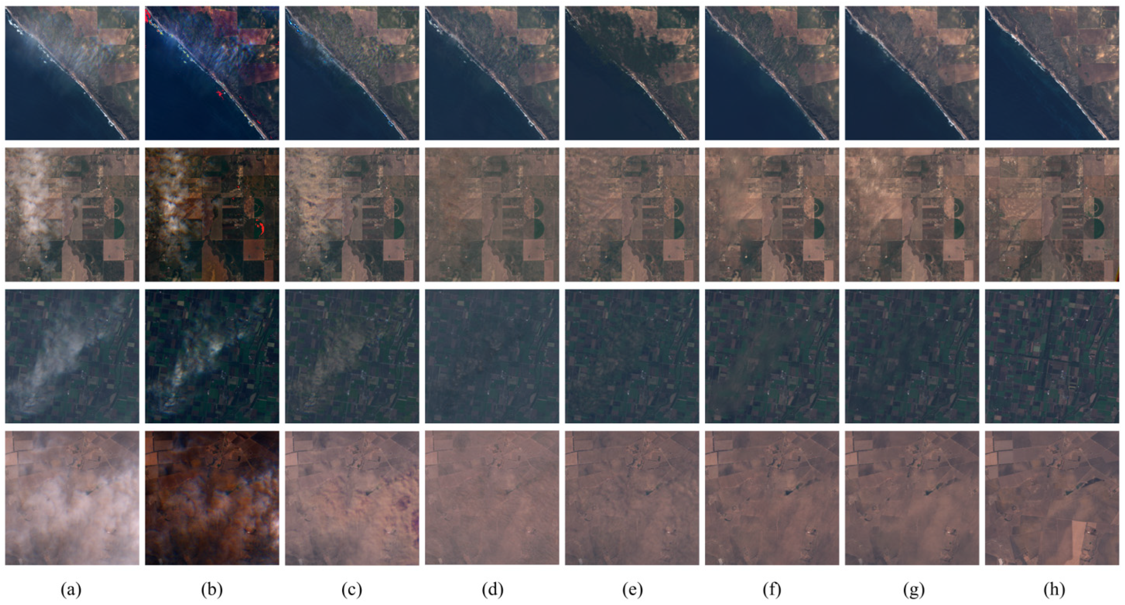
4.4. Qualitative Comparisons

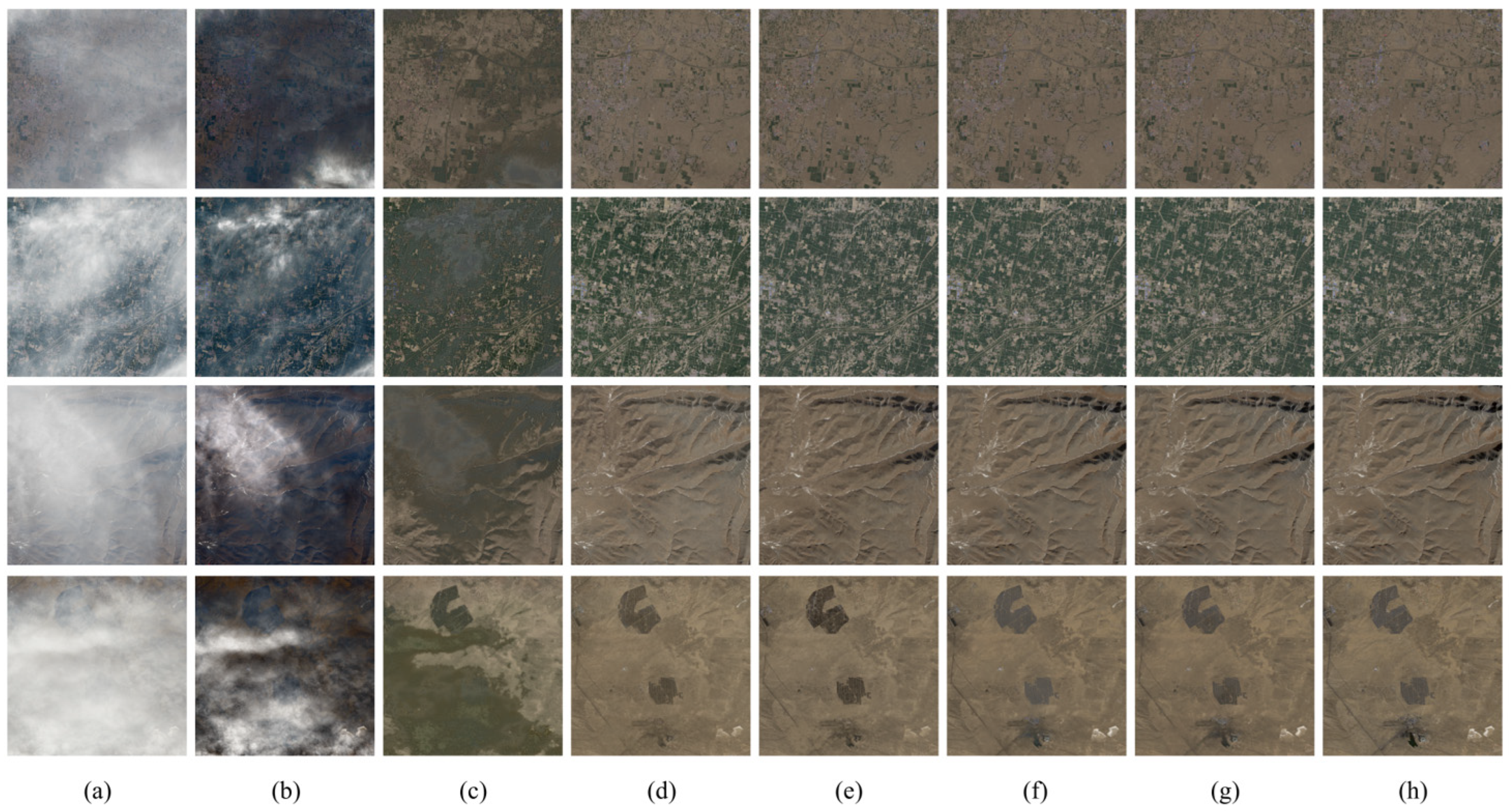
4.4.1. Qualitative Comparisons on RSHaze Dataset

Figure 7 showcases sample results of dehazing for all the methods tested on the RSHaze dataset. As observed in the figure, the DCP method enhances image quality to a degree by effectively removing thinner haze layers. However, it frequently leads to significant color distortion, culminating in an overall darker appearance of the image. AOD-Net, as depicted in the figure, addresses the color distortion issue, but it still exhibits a poor dehaze effect in regions with thick haze, an inadequate recovery of details, and noticeable textures of haze. The visual dehaze effects of GCANet, FCTF-Net, DehazeFormer, and our method, GLUENet, are already comparable, with only slight differences in fine texture in some areas. From this observation, it can be inferred that with the increasing number of model parameters, deep learning methods have reached a saturation point in terms of the dehazing effect on the synthetic dataset. This phenomenon arises due to the synthesis process of the dataset, wherein it is primarily generated using random transmittance maps with various random parameters. Subsequently, the atmospheric scattering equation for haze is applied to produce the haze image. This dictates the learning process of the deep learning network, which aims to learn the inverse solution process of this equation. Consequently, in the solution process of the finite unknown parameters, as the number of parameters in the deep learning model increases, the model’s performance reaching saturation becomes predictable. Further increasing the complexity of the model may improve performance metrics, but this often results in overfitting, adversely affecting generalization to real-world datasets.

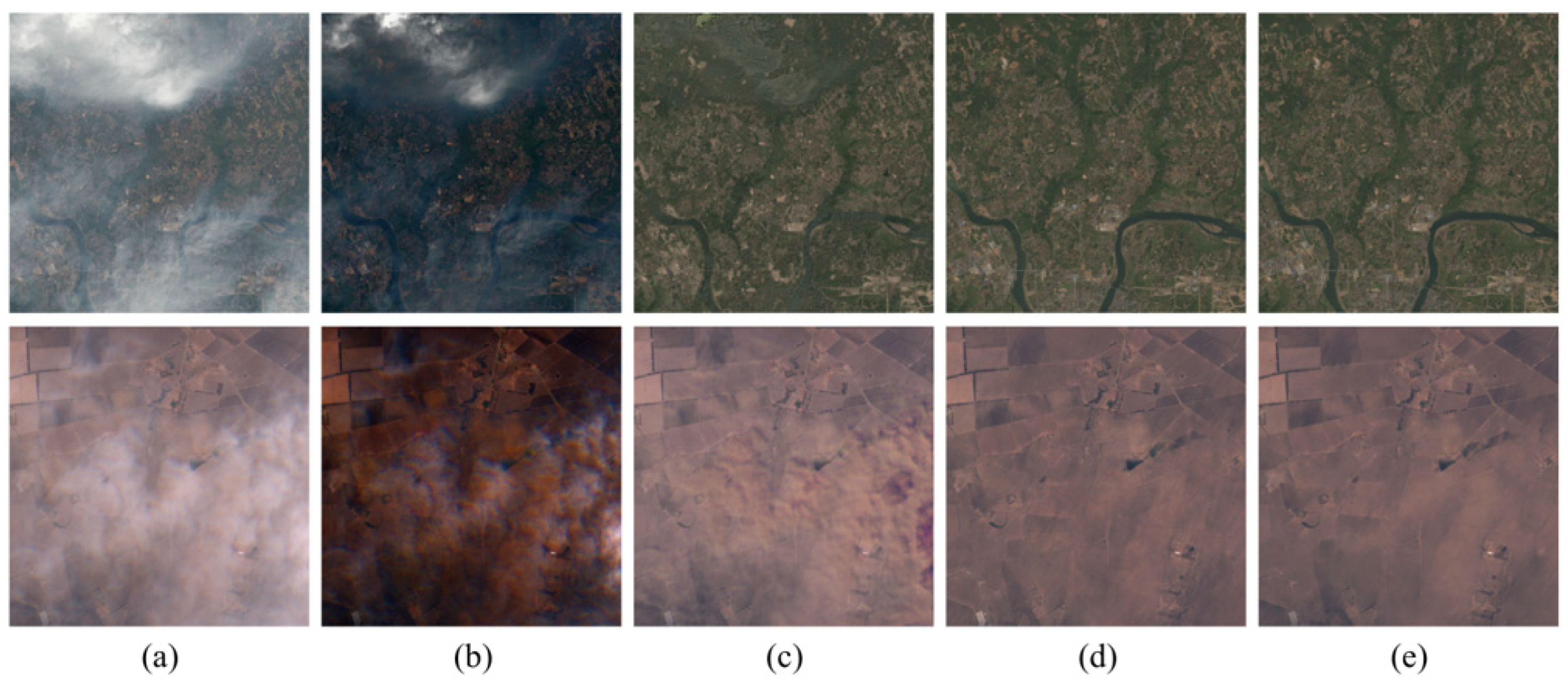
4.4.2. Qualitative Comparisons on RRSH Dataset

Figure 8 illustrates sample results of dehazing for all methods tested on the RRSH dataset. As evident from the figure, our dataset consists of authentic haze images, displaying significant variability in the dehazing effectiveness of each method. On the RRSH dataset, DCP demonstrates difficulty in eliminating the dense haze in the center, leading to an overall darker appearance of the image. AOD-Net, however, still retains a notable amount of haze texture. DehazeFormer and GLUENet surpass GCANet and FCTF-Net in terms of cloud haze removal, effectively eliminating the residual texture of dense haze in the cloud’s center and restoring a more natural and continuous appearance at the cloud boundary. Upon further comparison between DehazeFormer and our GLUENet method, it is observed that GLUENet can recover more detailed features, including buildings, cultivated land, and coastlines. Additionally, for areas covered by thick clouds, the colors recovered by our method appear more uniform and natural. Moreover, we notice that due to the ten-day interval between the acquisition of the hazy image and the clear image, there may be slight changes in the region. However, we believe that when the effective information in the dataset is sufficiently large, the small number of error pixels resulting from these changes can function similarly to noise, further enhancing the model’s generalization ability. In summary, our method accomplishes optimal visualization results on an authentic remote sensing dehazing image dataset, achieved with a model of relatively low complexity.

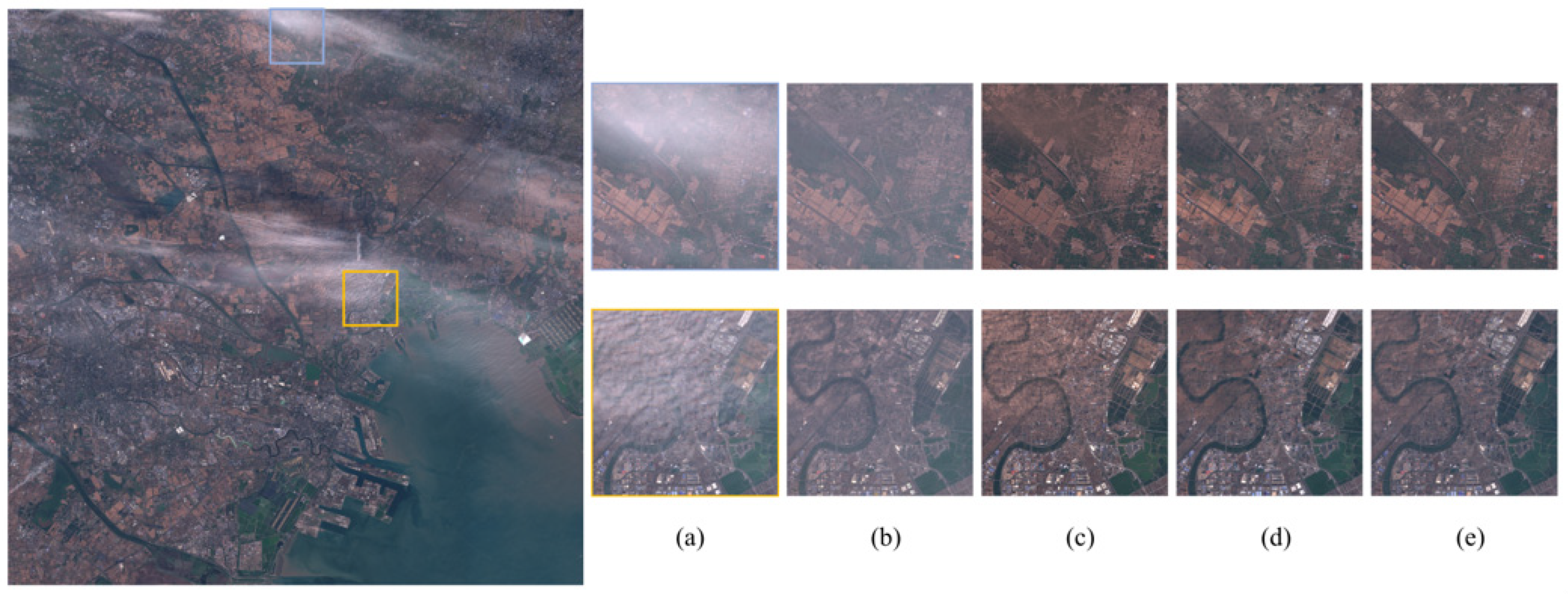
4.4.3. Qualitative Comparisons on Real Remote Sensing Images

To further evaluate the model’s generalization capabilities, we compare the dehazing effects of various deep learning dehazing algorithms on an entire scene of remote sensing imagery. The product ID of this specific Sentinel-2 image [48] under evaluation is S2A_MSIL1C_20231110T025931_N0509_R032_T50SNJ_20231110T044538 and the area where it was taken is located in the vicinity of Tianjin Port. Figure 9 illustrates the dehaze outcomes of GCANet, FCTF-Net, and DehazeFormer in the remote sensing image from a scene of Sentinel-2 remote sensing imagery with haze. On the right side of the figure, we present locally zoomed-in sections of the images post-dehazing using these methods, each covering a surface area of 10,240 m × 10,240 m. From the figure, it is evident that the overall whitening effect in the image after GCANet’s dehaze fails to capture the true color of the features. FCTF-Net exhibits difficulties in completely recovering surface features in areas shrouded by thick haze, leading to a significant loss of surface detail. Moreover, our method demonstrates the ability to recover clearer features, such as texture details of artificial facilities and buildings, in comparison to DehazeFormer. Additionally, the color rendition in the dehazed image by our method appears more natural and uniform overall. By leveraging mechanisms like GLU for extracting global information from the image, our method maintains robust performance on extensive remote sensing images, further affirming its generalization capabilities for remote sensing applications.

4.5. Ablation Analysis

To assess the efficacy of the GLUE block and the ECA Fusion module, we conduct an ablation study in this section. We compare the GLUENet variations listed below for this purpose.

The ‘plainnet’ in the table refers to a tandem model configuration, wherein the glu block is replaced by a sequence consisting of a 1 × 1 convolution, a depth-wise convolution, an activation function, and another 1 × 1 convolution. This model is utilized to benchmark the performance of the GLU module against a general baseline module.

To ensure a fair comparison, all model variants were trained following the same protocol as that used for GLUENet. The quantitative results of the dataset are shown in

Table 3. Quantitative comparison of variations of GLUENet on the RSHaze and RRSH dataset. For comparing methods, we use bold and italics to mark the best method.

Setting	RSHaze		RRSH		Overhead
	PSNR	SSIM	PSNR	SSIM	#Param (M)	MACs (G)
plainnet	37.62	0.969	32.98	0.933	1.42	4.60
+glu	37.67	0.970	33.16	0.935	1.42	4.38
+glu+eca	38.95	0.973	33.55	0.938	1.42	4.41
+glu+efusion	38.76	0.972	33.48	0.937	1.44	4.51
+glu+eca+efusion	38.98	0.973	33.57	0.938	1.44	4.62

. This shows that the ECA Fusion module of our proposed GLUE module is able to effectively aggregate spatial information and different stages to improve the dehazing performance of the baseline network.

4.5.1. Effectiveness of GLUE Block

Our GLUE module encompasses two pivotal components: the GLU mechanism and the ECA mechanism. In our ablation study, we initially examined the ECA mechanism alone, comparing models with and without the added ECA mechanism in Table 3. We observe a significant improvement in the performance of the network models with the added ECA mechanism. As the number of network layers deepens, the number of channels also increases, and the ability to interact with multi-channel information through the ECA mechanism facilitates the extraction of global information by the base module. When comparing the most basic GLU model with the general PlainNet model, we observe that the use of the GLU mechanism enhances network performance and concurrently reduces the amount of network computation, thereby accelerating the inference process. Hence, our GLUE module proves highly effective in global feature extraction and transformation.

4.5.2. Effectiveness of ECA Fusion

Upon comparing Table 3 with and without the inclusion of the ECA Fusion module, we observed an improvement in model performance with the addition of the ECA Fusion module. From the point of view of comparing the modules individually, ‘+glu+efusion’ compared to ‘+glu’, we can see that the efusion model is able to increase the performance of the model. However, when the ECA mechanism is added to the glu module, we find that the performance of the model is not significantly improved by adding efusion. The reason could be that both the GLUE module and the efusion module have an ECA mechanism. In our model, the number of layers in the base module is [2, 2, 2, 4], i.e., there are 20 GLUE blocks, while the number of efusion blocks is 3. Too many ECA mechanisms in the base module saturate the performance of the model. Our ECA Fusion module effectively integrates information from different stages, leveraging the retention of more haze texture information in the shallow features of the encoder. Weights are determined by feeding the encoder section’s low-level features and their matching high-level features into the ECA. The weights are then combined via the weighted summation technique. These operations enable the capturing of spatial distribution and morphological features of haze at a higher level, thereby enhancing the dehazing effect of non-uniform haze in remote sensing images.

5. Discussion

The task of dehazing remote sensing images presents a complex and formidable challenge in the field of image restoration. Due to advancements in deep learning techniques, an array of data-driven dehazing methods has emerged and been widely applied in the field of remote sensing. These methods encompass approaches based on CNN, Transformer architectures, and even the most recent diffusion models. Nonetheless, a discernible trend in SOTA methods is the adoption of increasingly intricate network structures and an expanding quantity of model parameters, benefiting from the fact that hardware capabilities are also advancing. While certain methods yield optimal results on specific test sets, they frequently feature significant inter-block and intra-block complexity within their network structures, with outcomes dependent on module stacking, thereby complicating the establishment of a standard baseline for comparison and reference among different methodologies. Furthermore, some modeling approaches necessitate a substantial number of parameters, posing difficulties for other researchers in reproducing these algorithms under limited hardware resources.

As a result, our approach is built on the core principles of simplicity and efficiency, and its effectiveness is well validated on both synthetic and real-world datasets. Experimental results show that the streamlined network architecture is able to obtain results comparable to those of the SOTA method, albeit with significantly lower computational overhead. Specifically, our architecture not only maintains a high level of performance when processing data but is also able to run at a much higher speed, which makes it more attractive for real-world applications.

In addition, our architecture reduces complexity, allowing other researchers to fully understand and compare the functionality of each of the constituent modules, thus facilitating their integration into various network designs. This simplified structure makes our approach easier to explain and understand, which in turn opens up broader possibilities for further research and applications. By clearly defining the functions and roles of each module, our approach provides a solid foundation for researchers to customize and extend across different tasks and domains. Overall, our method not only excels in performance but also has a simpler and clearer design, which provides a valuable tool for the machine learning community and helps accelerate the development and application of technologies in the field of remote sensing image dehazing.

However, our study is not devoid of limitations. Notably, there exists ample room for enhancement in the dehazing effect, especially in regions characterized by dense haze in real remote sensing contexts. Simultaneously, there is potential for further optimizations of our network structure, which could lead to a reduction in the number of parameters and computational requirements, without compromising the model’s performance. In our future work, we aim to enhance the dehazing effect by incorporating SAR (Synthetic Aperture Radar) images as auxiliary data, potentially resolving the recovery challenges in areas blanketed by thick haze. Additionally, with the increasing number of remote sensing satellites, it becomes feasible to construct larger and more diverse multi-scale remote sensing dehazing datasets. Looking forward, we plan to develop larger and more realistic datasets to thoroughly verify the generalizability of various dehazing methods.

6. Conclusions

We propose a simple, efficient, and new deep learning method called GLUENet for satellite remote sensing single-image dehazing. In comparison to natural hazy images, RS images consistently exhibit greater variability and inhomogeneity. Most prior deep learning methods rely on synthetic hazy datasets and enhance dehazing performance by layering various network modules. However, these methods often underperform in real-world remote sensing image dehazing scenarios, despite improvements in evaluation metrics on these datasets. On one hand, large model parameters can lead to overfitting, thereby affecting the model’s generalizability. On the other hand, they render the model training and deployment process heavily reliant on the capabilities of the computational device. To address this issue, we focus on two aspects: model construction and dataset formulation. Firstly, we leverage the mechanism of real remote sensing satellites revisiting the Earth’s surface every ten days to construct an authentic haze–no-haze dataset for model training. Regarding modeling, we have developed the GLUE module and the ECA Fusion module. The GLU within the GLUE module effectively captures the spatial distribution features of haze, while the ECA module adaptively obtains channel attention features. Simultaneously, the ECA Fusion module is capable of fusing information from various stages of the model. Experiments demonstrate that our proposed method performs comparably or even surpasses SOTA methods on RSHaze and RRSH, which are larger synthetic and real hazy datasets, while significantly reducing overhead.

References

1. Kotaridis, I.; Lazaridou, M. Remote Sensing Image Segmentation Advances: A Meta-Analysis. ISPRS J. Photogramm. Remote Sens. 2021, 173, 309–322. [Google Scholar] [CrossRef]
2. Jiang, H.; Peng, M.; Zhong, Y.; Xie, H.; Hao, Z.; Lin, J.; Ma, X.; Hu, X. A Survey on Deep Learning-Based Change Detection from High-Resolution Remote Sensing Images. Remote Sens. 2022, 14, 1552. [Google Scholar] [CrossRef]
3. Cheng, G.; Xie, X.; Han, J.; Guo, L.; Xia, G.-S. Remote Sensing Image Scene Classification Meets Deep Learning: Challenges, Methods, Benchmarks, and Opportunities. IEEE J. Sel. Top. Appl. Earth Obs. Remote Sens. 2020, 13, 3735–3756. [Google Scholar] [CrossRef]
4. He, K.; Sun, J.; Tang, X. Single Image Haze Removal Using Dark Channel Prior. IEEE Trans. Pattern Anal. Mach. Intell. 2011, 33, 2341–2353. [Google Scholar]
5. Zhu, Q.; Mai, J.; Shao, L. A Fast Single Image Haze Removal Algorithm Using Color Attenuation Prior. IEEE Trans. Image Process. 2015, 24, 3522–3533. [Google Scholar] [PubMed]
6. Berman, D.; Treibitz, T.; Avidan, S. Non-Local Image Dehazing. In Proceedings of the 2016 IEEE Conference on Computer Vision and Pattern Recognition (CVPR), Las Vegas, NV, USA, 27–30 June 2016; IEEE: Piscataway, NJ, USA, 2016; pp. 1674–1682. [Google Scholar]
7. Makarau, A.; Richter, R.; Muller, R.; Reinartz, P. Haze Detection and Removal in Remotely Sensed Multispectral Imagery. IEEE Trans. Geosci. Remote Sens. 2014, 52, 5895–5905. [Google Scholar] [CrossRef]
8. Li, B.; Peng, X.; Wang, Z.; Xu, J.; Feng, D. AOD-Net: All-in-One Dehazing Network. In Proceedings of the 2017 IEEE International Conference on Computer Vision (ICCV), Venice, Italy, 22–29 October 2017; IEEE: Piscataway, NJ, USA, 2017; pp. 4780–4788. [Google Scholar]
9. Li, Y.; Chen, X. A Coarse-to-Fine Two-Stage Attentive Network for Haze Removal of Remote Sensing Images. IEEE Geosci. Remote Sens. Lett. 2021, 18, 1751–1755. [Google Scholar] [CrossRef]
10. Qin, X.; Wang, Z.; Bai, Y.; Xie, X.; Jia, H. FFA-Net: Feature Fusion Attention Network for Single Image Dehazing. AAAI 2020, 34, 11908–11915. [Google Scholar] [CrossRef]
11. Song, Y.; He, Z.; Qian, H.; Du, X. Vision Transformers for Single Image Dehazing. IEEE Trans. Image Process. 2023, 32, 1927–1941. [Google Scholar] [CrossRef]
12. Shelhamer, E.; Long, J.; Darrell, T. Fully Convolutional Networks for Semantic Segmentation. IEEE Trans. Pattern Anal. Mach. Intell. 2017, 39, 640–651. [Google Scholar] [CrossRef]
13. Chen, L.; Chu, X.; Zhang, X.; Sun, J. Simple Baselines for Image Restoration. In Computer Vision—ECCV 2022; Lecture Notes in Computer Science; Springer Nature Switzerland: Cham, Switzerland, 2022; Volume 13667, pp. 17–33. ISBN 978-3-031-20070-0. [Google Scholar]
14. Zamir, S.W.; Arora, A.; Khan, S.; Hayat, M.; Khan, F.S.; Yang, M.-H. Restormer: Efficient Transformer for High-Resolution Image Restoration. In Proceedings of the 2022 IEEE/CVF Conference on Computer Vision and Pattern Recognition (CVPR), New Orleans, LA, USA, 21–24 June 2022; IEEE: Piscataway, NJ, USA, 2022; pp. 5718–5729. [Google Scholar]
15. Sandler, M.; Howard, A.; Zhu, M.; Zhmoginov, A.; Chen, L.-C. MobileNetV2: Inverted Residuals and Linear Bottlenecks. In Proceedings of the 2018 IEEE/CVF Conference on Computer Vision and Pattern Recognition, Salt Lake City, UT, USA, 18–23 June 2018; IEEE: Piscataway, NJ, USA, 2018; pp. 4510–4520. [Google Scholar]
16. Wang, Q.; Wu, B.; Zhu, P.; Li, P.; Hu, Q. ECA-Net: Efficient Channel Attention for Deep Convolutional Neural Networks. In Proceedings of the IEEE Conference on Computer Vision and Pattern Recognition (CVPR), Seattle, WA, USA, 13–19 June 2020. [Google Scholar]
17. Nayar, S.K.; Narasimhan, S.G. Vision in Bad Weather. In Proceedings of the Seventh IEEE International Conference on Computer Vision, Kerkyra, Greece, 20–25 September 1999; IEEE: Piscataway, NJ, USA, 1999; Volume 2, pp. 820–827. [Google Scholar]
18. Narasimhan, S.G.; Nayar, S.K. Removing Weather Effects from Monochrome Images. In Proceedings of the 2001 IEEE Computer Society Conference on Computer Vision and Pattern Recognition, CVPR 2001, Kauai, HI, USA, 8–14 December 2001; IEEE Computer Society: Washington, DC, USA, 2001; Volume 2, pp. II-186–II-193. [Google Scholar]
19. Cai, B.; Xu, X.; Jia, K.; Qing, C.; Tao, D. DehazeNet: An End-to-End System for Single Image Haze Removal. IEEE Trans. Image Process. 2016, 25, 5187–5198. [Google Scholar] [CrossRef] [PubMed]
20. Liu, Z.; Lin, Y.; Cao, Y.; Hu, H.; Wei, Y.; Zhang, Z.; Lin, S.; Guo, B. Swin Transformer: Hierarchical Vision Transformer Using Shifted Windows. In Proceedings of the 2021 IEEE/CVF International Conference on Computer Vision (ICCV), Montreal, QC, Canada, 10–17 October 2021; IEEE: Piscataway, NJ, USA, 2021; pp. 9992–10002. [Google Scholar]
21. Guo, J.; Yang, J.; Yue, H.; Tan, H.; Hou, C.; Li, K. RSDehazeNet: Dehazing Network with Channel Refinement for Multispectral Remote Sensing Images. IEEE Trans. Geosci. Remote Sens. 2021, 59, 2535–2549. [Google Scholar] [CrossRef]
22. Chen, Z.; Li, Q.; Feng, H.; Xu, Z.; Chen, Y. Nonuniformly Dehaze Network for Visible Remote Sensing Images. In Proceedings of the 2022 IEEE/CVF Conference on Computer Vision and Pattern Recognition Workshops (CVPRW), New Orleans, LA, USA, 21–24 June 2022; IEEE: Piscataway, NJ, USA, 2022; pp. 446–455. [Google Scholar]
23. Li, S.; Zhou, Y.; Xiang, W. M2SCN: Multi-Model Self-Correcting Network for Satellite Remote Sensing Single-Image Dehazing. IEEE Geosci. Remote Sens. Lett. 2023, 20, 1–5. [Google Scholar] [CrossRef]
24. Kulkarni, A.; Murala, S. Aerial Image Dehazing with Attentive Deformable Transformers. In Proceedings of the 2023 IEEE/CVF Winter Conference on Applications of Computer Vision (WACV), Waikoloa, HI, USA, 2–7 January 2023; IEEE: Piscataway, NJ, USA, 2023; pp. 6294–6303. [Google Scholar]
25. He, Y.; Li, C.; Li, X. Remote Sensing Image Dehazing Using Heterogeneous Atmospheric Light Prior. IEEE Access 2023, 11, 18805–18820. [Google Scholar] [CrossRef]
26. He, Y.; Li, C.; Bai, T. Remote Sensing Image Haze Removal Based on Superpixel. Remote Sens. 2023, 15, 4680. [Google Scholar] [CrossRef]
27. Zhao, S.; Zhang, L.; Shen, Y.; Zhou, Y. RefineDNet: A Weakly Supervised Refinement Framework for Single Image Dehazing. IEEE Trans. Image Process. 2021, 30, 3391–3404. [Google Scholar] [CrossRef] [PubMed]
28. Zhu, J.-Y.; Park, T.; Isola, P.; Efros, A.A. Unpaired Image-to-Image Translation Using Cycle-Consistent Adversarial Networks. In Proceedings of the 2017 IEEE International Conference on Computer Vision (ICCV), Venice, Italy, 22–29 October 2017. [Google Scholar]
29. Chen, X.; Fan, Z.; Li, P.; Dai, L.; Kong, C.; Zheng, Z.; Huang, Y.; Li, Y. Unpaired Deep Image Dehazing Using Contrastive Disentanglement Learning. In Computer Vision—ECCV 2022; Avidan, S., Brostow, G., Cissé, M., Farinella, G.M., Hassner, T., Eds.; Lecture Notes in Computer Science; Springer Nature Switzerland: Cham, Switzerland, 2022; Volume 13677, pp. 632–648. ISBN 978-3-031-19789-5. [Google Scholar]
30. Dauphin, Y.N.; Fan, A.; Auli, M.; Grangier, D. Language Modeling with Gated Convolutional Networks. In Proceedings of the 34th International Conference on Machine Learning, Sydney, NSW, Australia, 6 August 2017; Precup, D., Teh, Y.W., Eds.; PMLR—Proceedings of Machine Learning Research: Cambridge, MA, USA, 2017; Volume 70, pp. 933–941. [Google Scholar]
31. Shazeer, N. GLU Variants Improve Transformer. arXiv 2020, arXiv:2002.05202. [Google Scholar]
32. Tu, Z.; Talebi, H.; Zhang, H.; Yang, F.; Milanfar, P.; Bovik, A.; Li, Y. MAXIM: Multi-Axis MLP for Image Processing. In Proceedings of the IEEE/CVF Conference on Computer Vision and Pattern Recognition (CVPR), New Orleans, LA, USA, 18–24 June 2022; pp. 5769–5780. [Google Scholar]
33. Hendrycks, D.; Gimpel, K. Gaussian Error Linear Units (GELUs). arXiv 2016, arXiv:1606.08415. [Google Scholar]
34. Hu, J.; Shen, L.; Albanie, S.; Sun, G.; Wu, E. Squeeze-and-Excitation Networks. IEEE Trans. Pattern Anal. Mach. Intell. 2020, 42, 2011–2023. [Google Scholar] [CrossRef]
35. Woo, S.; Park, J.; Lee, J.-Y.; Kweon, I.S. CBAM: Convolutional Block Attention Module. In Proceedings of the European Conference on Computer Vision (ECCV), Munich, Germany, 8–14 September 2018. [Google Scholar]
36. Fu, J.; Liu, J.; Tian, H.; Li, Y.; Bao, Y.; Fang, Z.; Lu, H. Dual Attention Network for Scene Segmentation. In Proceedings of the IEEE/CVF Conference on Computer Vision and Pattern Recognition (CVPR), Long Beach, CA, USA, 15–20 June 2019. [Google Scholar]
37. Dosovitskiy, A.; Beyer, L.; Kolesnikov, A.; Weissenborn, D.; Zhai, X.; Unterthiner, T.; Dehghani, M.; Minderer, M.; Heigold, G.; Gelly, S.; et al. An Image Is Worth 16x16 Words: Transformers for Image Recognition at Scale. arXiv 2021, arXiv:2010.11929. [Google Scholar]
38. Bai, H.; Pan, J.; Xiang, X.; Tang, J. Self-Guided Image Dehazing Using Progressive Feature Fusion. IEEE Trans. Image Process. 2022, 31, 1217–1229. [Google Scholar] [CrossRef] [PubMed]
39. Schmitt, M.; Hughes, L.H.; Qiu, C.; Zhu, X.X. SEN12MS—A Curated Dataset Of Georeferenced Multi-Spectral Sentinel-1/2 Imagery For Deep Learning And Data Fusion. ISPRS Ann. Photogramm. Remote Sens. Spat. Inf. Sci. 2019, IV-2/W7, 153–160. [Google Scholar] [CrossRef]
40. Li, J.; Wu, Z.; Hu, Z.; Li, Z.; Wang, Y.; Molinier, M. Deep Learning Based Thin Cloud Removal Fusing Vegetation Red Edge and Short Wave Infrared Spectral Information for Sentinel-2A Imagery. Remote Sens. 2021, 13, 157. [Google Scholar] [CrossRef]
41. Drusch, M.; Del Bello, U.; Carlier, S.; Colin, O.; Fernandez, V.; Gascon, F.; Hoersch, B.; Isola, C.; Laberinti, P.; Martimort, P.; et al. Sentinel-2: ESA’s Optical High-Resolution Mission for GMES Operational Services. Remote Sens. Environ. 2012, 120, 25–36. [Google Scholar] [CrossRef]
42. Loshchilov, I.; Hutter, F. Decoupled Weight Decay Regularization. In Proceedings of the International Conference on Learning Representations, New Orleans, LA, USA, 6–9 May 2019. [Google Scholar]
43. Loshchilov, I.; Hutter, F. SGDR: Stochastic Gradient Descent with Warm Restarts. In Proceedings of the International Conference on Learning Representations, Touloun, France, 24–26 April 2017. [Google Scholar]
44. Wang, Z.; Bovik, A.C.; Sheikh, H.R.; Simoncelli, E.P. Image Quality Assessment: From Error Visibility to Structural Similarity. IEEE Trans. Image Process. 2004, 13, 600–612. [Google Scholar] [CrossRef] [PubMed]
45. Wang, Z.; Simoncelli, E.P.; Bovik, A.C. Multiscale Structural Similarity for Image Quality Assessment. In Proceedings of the Thrity-Seventh Asilomar Conference on Signals, Systems & Computers, Pacific Grove, CA, USA, 9–12 November 2003; IEEE: Piscataway, NJ, USA, 2003; pp. 1398–1402. [Google Scholar]
46. Zhang, L.; Zhang, L.; Mou, X.; Zhang, D. FSIM: A Feature Similarity Index for Image Quality Assessment. IEEE Trans. Image Process. 2011, 20, 2378–2386. [Google Scholar] [CrossRef]
47. Chen, D.; He, M.; Fan, Q.; Liao, J.; Zhang, L.; Hou, D.; Yuan, L.; Hua, G. Gated Context Aggregation Network for Image Dehazing and Deraining. arXiv 2018, arXiv:1811.08747. [Google Scholar]
48. Copernicus Browser. Available online: https://browser.dataspace.copernicus.eu/ (accessed on 29 February 2024).
Figure 1. A demonstration of our method’s outcomes compared to others. First row: synthesis haze. Second row: real haze. (a) Hazy images. (b) DCP. (c) AOD-Net. (d) DehazeFormer-B. (e) GLUENet (ours).
Remotesensing 16 01450 g001
Figure 2. Our proposed GLUENet is a simple U-Net variant. Compared to the conventional U-Net architecture, GLUENet uses GLUE blocks and an ECA Fusion module to replace the original convolutional blocks and concatenation fusion layers.
Remotesensing 16 01450 g002
Figure 3. Structure of the GLUE block.
Remotesensing 16 01450 g003
Figure 4. Structure of the Efficient Channel Attention.
Remotesensing 16 01450 g004
Figure 5. Structure of the Attention-Guided Fusion.
Remotesensing 16 01450 g005
Figure 6. Global distribution of the source images of our RRSH dataset.
Remotesensing 16 01450 g006
Figure 7. Qualitative comparisons on RSHaze. (a) Synthetic haze images. (b) DCP. (c) AOD-Net. (d) GCANet. (e) FCTF-Net. (f) DehazeFormer. (g) GLUENet (ours). (h) Ground-truth.
Remotesensing 16 01450 g007
Figure 8. Qualitative comparisons on RRSH. (a) Real haze images. (b) DCP. (c) AOD-Net. (d) GCANet. (e) FCTF-Net. (f) DehazeFormer. (g) GLUENet (ours). (h) Clear images.
Remotesensing 16 01450 g008
Figure 9. Qualitative comparisons on real RS image. (a) Real haze images. (b) GCANet. (c) FCTF-Net. (d) DehazeFormer. (e) GLUENet (ours). The box corresponds to the area where the detail on the right is in the large-scale remote sensing image on the left.
Remotesensing 16 01450 g009