Improved Landsat Operational Land Imager (OLI) Cloud and Shadow Detection with the Learning Attention Network Algorithm (LANA)

Abstract

Landsat cloud and cloud shadow detection has a long heritage based on the application of empirical spectral tests to single image pixels, including the Landsat product Fmask algorithm, which uses spectral tests applied to optical and thermal bands to detect clouds and uses the sun-sensor-cloud geometry to detect shadows. Since the Fmask was developed, convolutional neural network (CNN) algorithms, and in particular U-Net algorithms (a type of CNN with a U-shaped network structure), have been developed and are applied to pixels in square patches to take advantage of both spatial and spectral information. The purpose of this study was to develop and assess a new U-Net algorithm that classifies Landsat 8/9 Operational Land Imager (OLI) pixels with higher accuracy than the Fmask algorithm. The algorithm, termed the Learning Attention Network Algorithm (LANA), is a form of U-Net but with an additional attention mechanism (a type of network structure) that, unlike conventional U-Net, uses more spatial pixel information across each image patch. The LANA was trained using 16,861 512 × 512 30 m pixel annotated Landsat 8 OLI patches extracted from 27 images and 69 image subsets that are publicly available and have been used by others for cloud mask algorithm development and assessment. The annotated data were manually refined to improve the annotation and were supplemented with another four annotated images selected to include clear, completely cloudy, and developed land images. The LANA classifies image pixels as either clear, thin cloud, cloud, or cloud shadow. To evaluate the classification accuracy, five annotated Landsat 8 OLI images (composed of >205 million 30 m pixels) were classified, and the results compared with the Fmask and a publicly available U-Net model (U-Net Wieland). The LANA had a 78% overall classification accuracy considering cloud, thin cloud, cloud shadow, and clear classes. As the LANA, Fmask, and U-Net Wieland algorithms have different class legends, their classification results were harmonized to the same three common classes: cloud, cloud shadow, and clear. Considering these three classes, the LANA had the highest (89%) overall accuracy, followed by Fmask (86%), and then U-Net Wieland (85%). The LANA had the highest F1-scores for cloud (0.92), cloud shadow (0.57), and clear (0.89), and the other two algorithms had lower F1-scores, particularly for cloud (Fmask 0.90, U-Net Wieland 0.88) and cloud shadow (Fmask 0.45, U-Net Wieland 0.52). In addition, a time-series evaluation was undertaken to examine the prevalence of undetected clouds and cloud shadows (i.e., omission errors). The band-specific temporal smoothness index (TSI_λ) was applied to a year of Landsat 8 OLI surface reflectance observations after discarding pixel observations labelled as cloud or cloud shadow. This was undertaken independently at each gridded pixel location in four 5000 × 5000 30 m pixel Landsat analysis-ready data (ARD) tiles. The TSI_λ results broadly reflected the classification accuracy results and indicated that the LANA had the smallest cloud and cloud shadow omission errors, whereas the Fmask had the greatest cloud omission error and the second greatest cloud shadow omission error. Detailed visual examination, true color image examples and classification results are included and confirm these findings. The TSI_λ results also highlight the need for algorithm developers to undertake product quality assessment in addition to accuracy assessment. The LANA model, training and evaluation data, and application codes are publicly available for other researchers.

1. Introduction

The Landsat satellite series provides the longest record of land observations from space, and the >10 million images sensed since 1972 are archived and processed by the United States Geological Survey (USGS) into radiometrically calibrated, geolocated, and atmospherically corrected images [1]. The most recently processed Collection 2 Landsat data sensed by the Thematic Mapper (TM) (Landsat 4 and 5), Enhanced Thematic Mapper Plus (ETM+) (Landsat 7), Operational Land Imager (OLI), and Thermal Infrared Sensor (TIRS) (Landsat 8 and 9) instruments are provided with cloud and shadow masks so that contaminated pixels may be discarded prior to analysis [2]. Accurate cloud and shadow classification is challenging, particularly over cold and highly reflective surfaces, or over dark surfaces, that are spectrally similar to clouds and shadows, respectively [3,4,5,6]. The need for improved Landsat cloud detection in the next Landsat collection has been recognized [2]. In this paper, we present research to develop improved cloud and cloud shadow masking suitable for global application to Landsat OLI data using a recent deep learning attention model.

The Landsat sensors were not designed for cloud property investigations and lack the appropriate spectral bands and sensor design found on dedicated cloud and atmospheric satellite remote sensing systems [7,8,9,10]. Consequently, physically based cloud and cloud shadow detection algorithms have not been developed for Landsat, and instead, algorithms have used supervised classification or empirical spectral test-based approaches. Clouds are dynamic with considerable spatial, seasonal, and diurnal variation; have variable morphology, water vapor content, and height; and often co-exist at different altitudes [11,12,13]. Consequently, conventional supervised classification algorithms that are applied to individual Landsat pixels, using classifiers such as decision trees [14,15,16], artificial neural networks [16,17], and random forests [18,19], are challenging to train in a globally representative manner and apply to provide globally reliable results. A number of empirical cloud detection algorithms have been developed that apply spectral tests to individual Landsat pixels [20,21,22,23,24]. Cloud shadow detection algorithms have also been developed and typically first require a cloud mask and use the sun-cloud-sensor geometry with an assumed or approximately estimated cloud height (based on brightness temperature for Landsat sensors with thermal bands) to locate potentially shaded areas, followed by spectral tests to refine the locations of shadow pixels [25,26,27,28]. In addition, algorithms using time series images have also been developed by assuming that cloud changes more rapidly than land surface [4,6,29,30]). The Landsat cloud and cloud shadow masks are generated using a version of the empirical Fmask cloud and cloud shadow detection algorithms [2].

In the last decade, a number of deep learning algorithms using convolutional neural networks have been developed for Landsat cloud and cloud shadow detection (summarized in Appendix A). Rather than be applied to individual pixels, they are applied to square image subsets, termed patches, and the spatial relationships within the patch provide additional information for cloud and shadow detection. The trained network is applied to image patches translated across the image to classify each patch center pixel. Fully convolutional networks (FCN) [31] classify all the patch pixels, rather than the center pixel, and most recent Landsat cloud/shadow deep learning architectures use some form of FCN [32,33]. In particular, the U-Net model has been adopted because it preserves spatial detail by using skip connections between low-level and high-level features [34]. For example, [32,33,35,36,37,38] used U-Net for cloud detection, although other architectures such as SegNET [39] and DeepLab [40] have also been used. Most models are implemented with patch spatial dimensions varying from 86 × 86 to 512 × 512 30 m pixels and using the OLI visible and short wavelength bands. Of the deep learning algorithms summarized in Appendix A, only a minority also used the TIRS bands. Deep learning algorithms that detect clouds and shadows separately have been developed [41,42] although this may result in the incorrect detection of both cloud and cloud shadows at the same pixel location. All the Landsat deep learning algorithms summarized in Appendix A were trained and evaluated using publicly available annotated datasets derived by visual interpretation of 185 × 180 km Landsat images [22] or image spatial subsets [17].

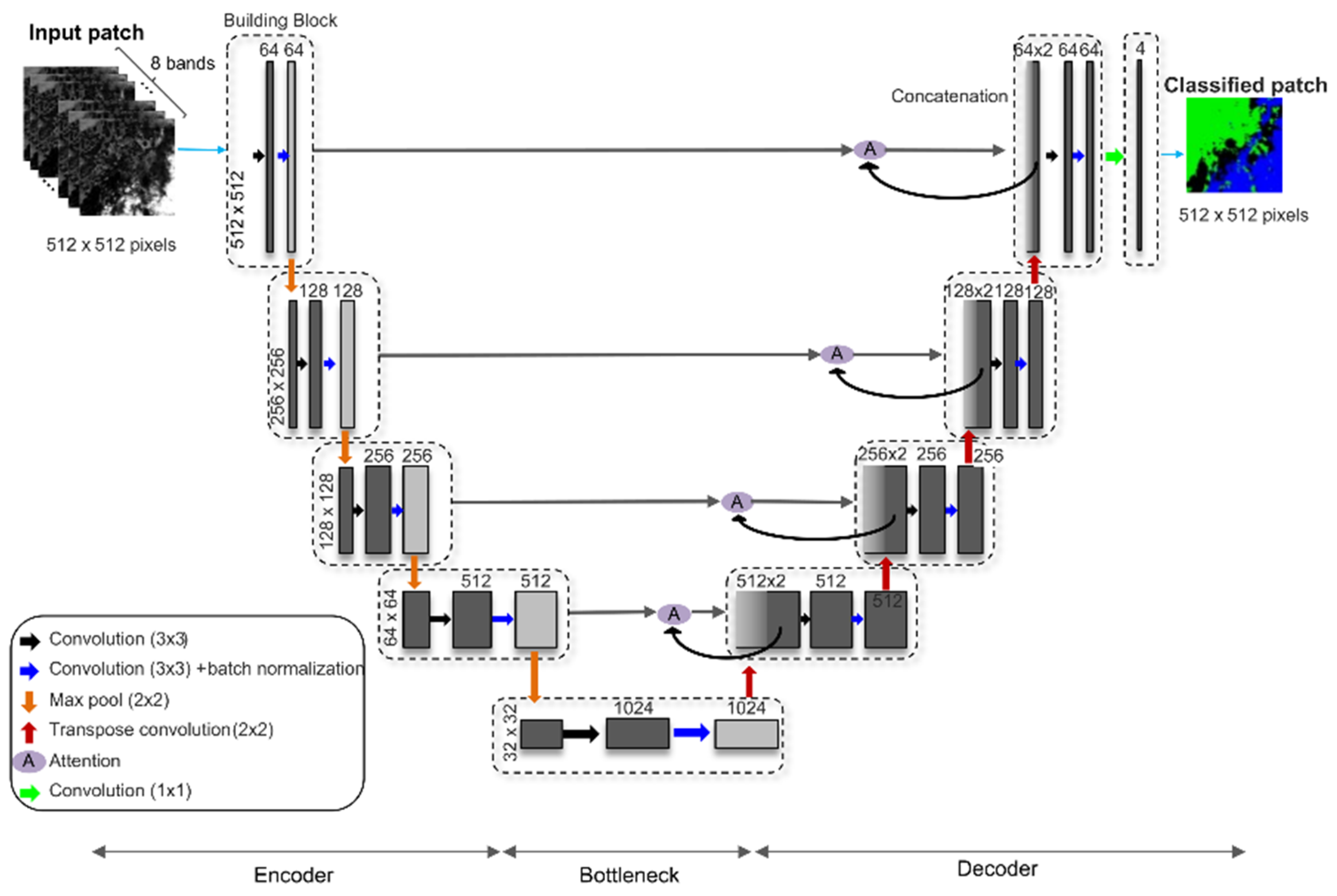
We present a new Landsat 8/9 OLI cloud and cloud shadow masking algorithm that classifies pixels as either clear, thin cloud, cloud, or cloud shadow. The algorithm is called the Learning Attention Network Algorithm (LANA) and is designed for application to OLI imagery acquired over global land surfaces, including snow and coastal/inland water. The LANA is a form of U-Net with an additional attention mechanism that reduces small receptive field (a small local spatial window around a patch pixel that determines the feature values for the pixel) issues. The issues often present in convolution-based deep learning structures are that the feature values for a pixel location in a two-dimensional feature map (derived by a convolutional layer) may be determined by only a small local spatial window around the pixel [43,44]. The attention mechanism was developed to capture long-range structure among pixels [45,46] in image classification, which was inspired by the attention success in machine translation each word generation needs to attend to all the input words in the to-be-translated sentence to address the grammar difference [47,48]. This may be helpful for detection of cloud shadows that always occur to the west of clouds in Landsat imagery because the sun is in the East for the majority of global land areas except at very high latitudes due to the Landsat morning overpass time [49]. The offsets can be quite large relative to 30 m pixel dimensions. For example, shadows will be offset from clouds by 3.76 km and 6.92 km, considering a cloud with a global average 4.0 km cloud top height [11] and solar zenith angles of 43.23° and 60°, respectively. The global annual mean Landsat solar zenith angle is 43.23° and a 60° solar zenith angle is typically experienced in Landsat imagery at mid-latitudes in the winter [49]. The attention mechanism may also be helpful for cloud detection in images with non-random cloud distributions. A customized loss function was also used in the LANA implementation to increase the influence of minority classes in the model training that can be missed by machine learning models [50,51].

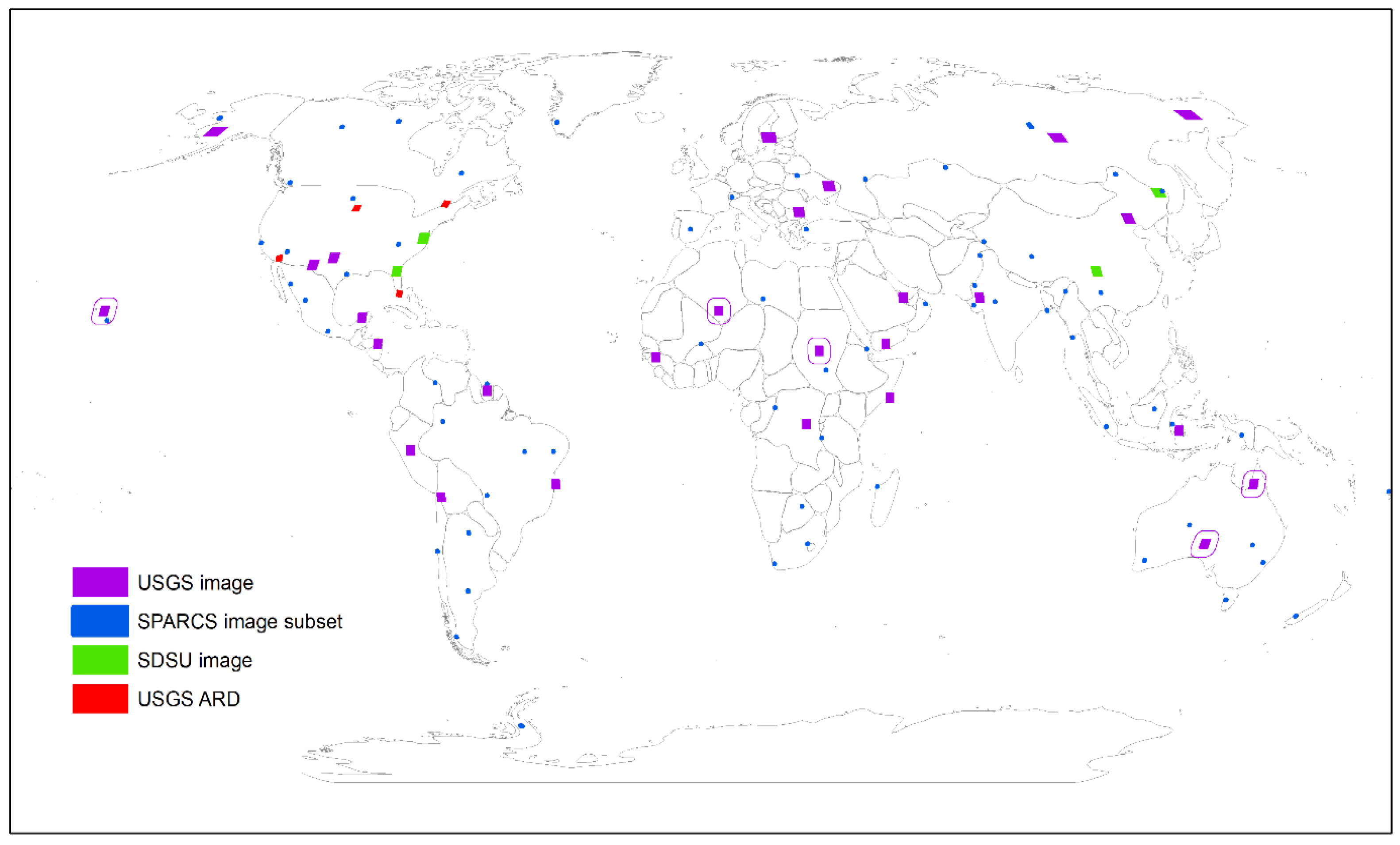
The LANA was trained using Landsat 8 OLI top of atmosphere (TOA) reflectance and associated cloud/shadow state annotations drawn from a pool of 100 datasets composed of (i) 27 Landsat 8 images annotated by USGS personnel [52], (ii) 69 1000 × 1000 Landsat 8 image subsets annotated by the Spatial Procedures for Automated Removal of Cloud and Shadow (SPARCS) project [17], and (iii) 4 Landsat 8 images that we annotated to capture image conditions underrepresented in the USGS and SPARCS datasets. Overall and class-specific accuracy statistics were derived from a single confusion matrix populated with the five selected datasets from the 100 datasets. For comparative purposes, the classification accuracies provided by a conventional U-Net model [36], referred to here as U-Net Wieland, were also assessed. The U-Net Wieland model was considered as its authors have publicly released their trained model, mitigating potential implementation biases that may arise from re-training other published models. This is a real issue, as deep learning model performance is sensitive to the implementation and hyper-parameter settings [53,54]. The accuracy of the Fmask cloud/shadow mask provided with the Landsat 8 data was quantified, considering the same evaluation data as a benchmark.

In addition to cloud and cloud shadow accuracy assessment, the results of the three algorithms (LANA, U-Net Wieland, and Fmask) were compared considering a year of Landsat 8 OLI data acquired over four 5000 × 5000 30 m Landsat Analysis Ready Data (ARD) tiles [55]. The geographic coordinates of each Landsat ARD tile pixel are fixed, and no additional geometric alignment steps are necessary prior to multi-temporal analysis using the ARD. Qualitative visual comparisons were undertaken, and summary statistics of the number of cloud and shadow masked observations over the year for the algorithms were compared. The temporal smoothness of the cloud and shadow-masked ARD surface reflectance time series was quantified to provide insights into the relative prevalence of undetected clouds and cloud shadows.

The paper is structured as follows. First, the Landsat 8 training and evaluation data are described (Section 2). Then, the methods, including the LANA algorithm, accuracy assessment, and the algorithm time-series comparison, are described (Section 3). This is followed by the results (Section 4) reporting the LANA training and parameter optimization, accuracy assessment, and algorithm comparisons. The paper concludes with a discussion of LANA and its merits over the two other cloud and cloud shadow masking algorithms.

2. Landsat Training and Evaluation Data

2.1. Landsat Operational Land Imager (OLI) Sensor

The Operational Land Imager (OLI) is on the Landsat 8 and Landsat 9 satellites. Landsat 8 was launched in 2013 into a sun synchronous 705 km orbit with a 10:12 am Equatorial overpass time and carries the OLI and the Thermal Infrared Sensor (TIRS) [56]. The Landsat 9 satellite was launched in 2021 into the same orbit with an 8-day phase difference as Landsat 8 and carrying the same sensors; notably, the Landsat 9 OLI is a clone of the Landsat 8 OLI [57]. The OLI acquires 30 m data in eight reflective wavelength bands: coastal blue 0.43–0.45 µm, blue 0.45–0.51 µm, green 0.53–0.59 µm, red 0.64–0.67 µm, near infrared (NIR) 0.85–0.88 µm, short-wave infrared (SWIR-1) 1.57–1.65 µm, SWIR-2 2.11–2.29 µm, and cirrus 1.36–1.38 µm. The TIRS acquires 100 m data in two thermal bands (10.60–11.19 μm and 11.50–12.51 μm).

2.2. Landsat OLI Images and ARD

Landsat 8 OLI images and OLI ARD provided by the USGS [58] were used in this study. The OLI images cover ~185 × 180 km and are defined in the Universal Transverse Mercator (UTM) projection referenced by the Worldwide Reference System-2 (WRS-2) path (along track direction) and row (across track direction) coordinate system [2]. The OLI ARD are derived by application of the same processing algorithms as for the images but are defined (without double resampling) in the Albers equal area projection in fixed non-overlapping 5000 × 5000 30 m pixel (150 × 150 km) tiles referenced by horizontal (h) and vertical (v) tile coordinates [55]. Each individual Landsat orbit overlapping an ARD tile is stored independently. The geographic coordinates of each ARD tile pixel are fixed, and only images that can be geolocated with <12 m RMSE are used to generate the ARD, and so the ARD support straight-forward time-series analysis [55]. The Landsat 8 OLI images and ARD are provided with per-pixel quality flags, including radiometric saturation and Fmask cloud/shadow flags. The radiometric saturation flag defines the saturation status of each band. The Fmask algorithm (described in Section 3.4) labels each 30 m pixel observation as cloud, cloud shadow, cirrus, or clear.

The USGS has periodically reprocessed the Landsat archive in recognition of the need for more consistently processed Landsat data. All USGS Landsat data released prior to 2017 are referred to as pre-Collection data. The Landsat images and ARD were reprocessed as Collection 1 in 2017 and then reprocessed again as Collection 2 in 2020 [2]. The Collection 1 data were processed using more up-to-date calibration but have the same geolocation as the pre-collection data. The Collection 2 data have a number of improvements over Collection 1, summarized in [2], most notably improved geolocation due to the availability of new European Space Agency ground control data [59,60]. These collection geolocation differences are important because of the need to ensure meaningful alignment of the annotated cloud/shadow data and Landsat 8 OLI data used in this study.

2.3. Annotated Cloud and Cloud Shadow Datasets

To undertake the training and accuracy assessment, a pool of 100 sets of annotated Landsat 8 OLI data was used. The pool is globally distributed (Figure 1) and covers a range of surface types and cloud covers. The pool is composed of (i) 27 USGS-supplied cloud and shadow annotated Landsat 8 images [52], (ii) 69 annotated 1000 × 1000 Landsat 8 image subsets defined by the Spatial Procedures for Automated Removal of Cloud and Shadow (SPARCS) dataset [17], and (iii) 4 annotated Landsat 8 images (a completely cloudy image, a partially clear image acquired over an urban area, and two completely clear images) that we annotated by careful visual inspection and that were selected to capture conditions underrepresented in the USGS and SPARCS datasets. For convenience, we refer to these four images as South Dakota State University (SDSU) images.

The USGS and SPARCS annotations were derived from pre-Collection imagery, and so, as they have the same geometry as Collection 1, we transferred their annotations to the corresponding Collection 1 Landsat 8 OLI imagery. No Collection 2 images were used to minimize any potential misregistration with the pre-Collection annotations. The four SDSU annotations were purposefully generated using Collection 1 imagery to be consistent. Small spatial coverage mismatches that can occur at the image swath edges between the Collection-1 and pre-Collection data (due to differences in handling the staggered spectral band readout at the image edges, see Figure 1c in [61]) were resolved by clipping so that only the spatially intersecting areas of the pre-Collection and Collection-1 images were retained.

The USGS annotated 32 Landsat 8 OLI images to define each 30 m pixel as cloud, thin cloud, cloud shadow, or clear [52]. The dataset included images with missing cloud shadow annotations, and five images had visually indistinguishable cloud and snow areas that were unlikely to have been annotated perfectly, so they were discarded to leave a total of 27 annotated USGS images (Figure 1, purple). Eight of the 27 USGS images had cloud shadows not annotated over water, and two had thin clouds that were incorrectly annotated, so we refined their annotations. The SPARCS annotations define 30 m pixels as shadow, shadow over water, water, snow, land, cloud, or flooded [17]. We reclassified these seven classes into four classes (cloud, thin cloud, cloud shadow, or clear) by combining the water, land, flooded, and snow classes as clear, and combining the shadow and shadow over water classes as cloud shadow. Ten of the SPARCS 1000 × 1000 30 m pixel subsets had unreliable annotations and were removed to leave 69 subsets (Figure 1 cyan). The four SDSU annotated Landsat 8 images (Figure 1, green) were composed of a completely cloudy image, two completely clear images, and a partially clear image over an urban area and were included as these conditions were underrepresented in the USGS and SPARCS annotated data. The completely cloudy image was sensed over the eastern U.S. and was selected because it contained a variety of cloud spatial textures. The two completely clear images were sensed over a low-reflectance forested area in the southeast U.S. and over a highly reflective snow-covered area in northeast China. The partially clear urban image was sensed over the Seoul metropolitan area in South Korea and contained a complex of cloud, thin cloud, cloud shadow, and clear pixels.

2.4. Training Patch Extraction

A total of 16,861 512 × 512 30 m pixel training patches (

Table 1. Summary of the training 512 × 512 30 m pixel patches extracted from the annotated data.

Dataset	Number of Landsat 8 Images	Number of Patches
USGS	27 images	14,586
SPARCS	69 1000 × 1000 30 m pixel image subsets	621
SDSU	4 images	1654

) were extracted from the 100 annotated datasets. The patches were extracted by translating a 512 × 512 pixel window in steps (i.e., strides) of every 256 pixels in the x and y axes, and only patches completely containing observations (no unsensed pixels) were retained. This was straightforward to implement for the SPARCS 1000 × 1000 30 m pixel square image subsets. However, due to the inclined orientation of the Landsat images, the number of training patches that could be extracted from the USGS and SDSU annotated imagery was maximized by staggering the patch locations. Data augmentation techniques such as flipping and rotating patches [62] were not used because they do not preserve the systematic westward offset of cloud shadows relative to clouds observed in Landsat imagery. Each patch was composed of the eight Landsat 8 OLI TOA reflectance (coastal blue, blue, green, red, NIR, SWIR-1, SWIR-2, and cirrus) bands. The OLI radiometric saturation status was not considered as, unlike earlier Landsat sensor data, the OLI reflective wavelength bands are rarely saturated [63]. The two TIRS thermal bands (10.60–11.19 μm and 11.50–12.51 μm), which are provided in 30 m resampled from the acquired 100 m resolution [2], were not used as we experimentally found that their use negatively impacted the classification performance (discussion).

2.5. Unannotated Landsat 8 ARD Time Series

Differences among the three algorithms (LANA, U-Net Wieland, and Fmask) were examined considering all the Collection 2 Landsat 8 OLI ARD reflectance acquired in 2021 at four ARD tiles. The tiles (Figure 1 red) were selected across the conterminous United States (CONUS) to encompass different land surfaces and cloudiness and to not coincide with any of the 100 annotation data. Figure 2 illustrates the four tiles showing the median red, green, and blue (true color) reflectance derived over the summer (May to September 2021).

Table 2. Summary of the four Landsat ARD horizontal and vertical tile coordinates, the tile geographic locations, and the number of days that the tile was observed by Landsat 8 from 1 January to 31 December 2021. The last two columns show the total number of tile 30 m pixel observations (pixels with OLI reflectance), and the percentage labeled by the Collection 2 Fmask as cloud or cloud shadow, for 1 January to 31 December 2021.

ARD Tile	Location	Numbers of Days in 2021 with Observations	Total Number of 30 m Pixel Observations in 2021	Percentage of Tile 30 m Pixel Observations in 2021 Flagged as Cloud and Cloud Shadow
h28v04	Canada/US	45	819,622,208	65.75
h05v13	Mexico/US	46	765,724,406	22.54
h15v06	South Dakota	68	831,168,336	45.31
h27v19	Florida	46	653,119,627	46.93

summarizes for each tile the number of days in 2021 with tile observations, i.e., when some or all of the 5000 × 5000 30 m ARD tile pixels were sensed by Landsat 8 (regardless of cloud or cloud shadow state), and the number of days varied among the four tiles from 45 to 68 days. These count values are greater for the higher latitude tiles (smaller vertical tile coordinate values) because the Landsat swaths converge further northward [64]. The total number of tile 30 m pixel Landsat 8 OLI observations (regardless of cloud and shadow status) over the year varied from approximately >660 to >830 million tile pixel observations. The percentage of tile pixel observations identified by the Fmask as cloud or cloud shadow varied by a factor of three from 22.5% (Mexico/US) to 65.7% (Canada/US) and was intermediate at 45.3% (Florida) and 46.9% (South Dakota) for the other two tiles.

The Canada/US and Mexico/US tiles were selected because they were found to be the least and most observed ARD tiles across the CONUS based on examination of all the Landsat 4, 5, and 7 ARD for 1982 to 2017 (36 years) [65]. The least observed tile (h28v04) is located on the Canada–US border encompassing Quebec, Vermont, and New York states, and includes forest, cropland, and urban land covers (greater Montreal area) and water, including the St. Lawrence River flowing southwest to northeast and Lake Ontario in the southwest (Figure 2a). The most observed tile (h05v13) is located on the Mexico–US border, encompassing Baja California, Mexico, and southern California and Arizona, and includes areas of dryland shrubs, desert, and irrigated croplands (Figure 2b). Two ARD tiles that we examined in previous studies [61,66,67] were also considered. They are an urban and coastal tile (h27v19) encompassing the Miami metropolitan area, wetlands (the Everglades water), and water (the Straits of Florida) (Figure 2d), and an agricultural tile (h15v06) in South Dakota that is covered predominantly by cropland and grassland with the Missouri river running from north to south and that is often snow covered in the winter (Figure 2c).

3. Methods

3.1. Learning Attention Network Algorithm (LANA)

Figure 3 illustrates the LANA structure used to classify each pixel of a 512 × 512 30 m pixel patch as cloud, thin cloud, cloud shadow, or clear. Following the conventional U-Net structure, the LANA has three main parts—an encoder, a bottleneck, and a decoder [34]. The encoder is directly connected to the input 8-band reflectance image patch. It consists of four convolutional blocks, with each resulting in c_k m_k × m_k feature maps storing feature values (m_k × m_k × c_k) (k = 1, 2, 3, and 4 representing the four convolutional blocks), where m_k = 512/2^k. The feature map is reduced by a factor of two in each dimension because 2 × 2 max-pooling was used to suppress irrelevant information (by selecting the maximum value from 2 × 2 windows across each feature map). The four ck values were set as 64, 128, 256, and 512, respectively, i.e., the feature map number increases with decreasing feature map dimensions to maintain a similar amount of information typically used in U-Net models [34,68]. Each convolution block consists of two 3 × 3 kernel convolution layers, followed by a batch normalization layer. The bottleneck consists of one convolution block with 1024 feature maps. The decoder consists of four convolutional blocks, each starting with a transpose convolutional layer and resulting in c_k′ m_k′ × m_k′ feature maps storing feature values (m_k′ × m_k′ × c_k′) (k′ = 1, 2, 3 and 4 representing the four decoder convolutional blocks). The transpose convolution layer is used to increase the size of the feature maps by 2 in each dimension. The transpose convolution layer is implemented by inserting a column/row of 0 values after each column/row of feature maps to expand by 2 in each dimension and then applying a 2 × 2 convolution. The four c_k′ values derived in the decoder were set as 512, 256, 128, and 64, respectively, to mirror the encoder implementation. The feature maps derived from the last decoder convolution layer are applied by a 1 × 1 convolution with a softmax activation function to derive the probability of each class for each patch pixel. All the encoder, bottleneck, and decoder convolutional layers used the rectified linear unit (ReLU) activation function so that any negative values were set to zero and positive values remained unchanged [69].

The U-Net has skip connections (Figure 3 horizontal gray lines) in the encoder–decoder architecture so that high spatial resolution information that is progressively smoothed in the encoder layers is recovered in the decoder layers. Conventionally, U-Net skip connections are used to copy feature maps from the encoder (Figure 3, light gray rectangles) to their decoder block counterparts. The attention mechanism was implemented in the LANA by transforming the encoder feature maps when they are copied to the decoder side in the skip connections. The attention mechanism is described below.

The attention mechanism was developed to increase the effective receptive field in convolutional networks [45,46]. In convolution-based structures, such as U-Net, the feature values for a patch pixel location are determined by a small local spatial window around the pixel, termed the receptive field. The receptive field contribution to the classification output is greatest in the center and decreases rapidly towards the receptive field edges [44] and can be modelled by the radius of a Gaussian function beyond which the contribution is negligible [43]. For example, a U-Net with the same architecture as LANA but without attention has a receptive field of 140 × 140 pixels and an effective receptive field that can be approximated by a circular region with a radius of less than only 13 pixels [70]. The receptive field size increases with the number of convolutional, max-pooling, and transpose convolution layers [44,71,72]. The attention mechanism is implemented by transforming each feature into a feature map to a new feature derived as a weighted combination of all the features in the feature map. The attention weights are defined using similarity scores among the features in a linearly transformed space, and so this process is usually called self-attention as the feature map itself is used to calculate the weights [45,46].

The attention mechanism was implemented in the LANA (shown by the black curved arrows in Figure 3) by transforming the encoder feature maps as they are copied to the decoder side. There are c feature maps (for example, c = 64 in the top layer in Figure 3), and each has two dimensions with m × m elements (for example, m = 512 in the top layer in Figure 3). The transformed encoder feature map is derived [45] as:

$$f_i^{\prime }=\gamma {\mathit{W}}_{\mathit{v}}({\sum }_j^{m^2}{a_{ij}{\mathit{W}}_{\mathit{h}}f}_j)+f_i (i=1,2,\dots ,m^2)$$

(1)

$$a_{ij}=\frac{\exp \left({\mathit{W}}_{\mathit{g}}{g}_j{({\mathit{W}}_{\mathit{f}}{f}_i)}^T\right)}{{\sum }_i^{m^2}\exp \left({\mathit{W}}_{\mathit{g}}{g}_j{({\mathit{W}}_{\mathit{f}}{f}_i)}^T\right)}$$

(2)

where $f_i^{\prime }$ and $f_i$ are feature vectors (each 1 × c) at position i (1, 2, …, m²) in the c feature maps after and before applying the attention model, and γ is a learnable scalar value initialized as 0 and is used to gradually increase the attention model contributions in the training. The terms ${\mathit{W}}_{\mathit{h}}$ ($\overline{c}$ × c) and ${\mathit{W}}_{\mathit{v}}$ (c × $\overline{c}$) are two learnable coefficient matrices, a_ij is the attention weight indicating the extent to which the ith position attends to the jth position, g_j is another feature vector at position j (1 × c) from the decoder m × m × c feature maps that the encoder feature maps are copied over, and W_f ($\overline{c}$ × c) and W_g (c × $\overline{c}$) are two learnable coefficient matrices. The convolution block symbol k is omitted in Equations (1) and (2) as the attention model was applied to all encoder feature maps derived from the four convolution blocks (Figure 3). The bias coefficients normally following the weight coefficients are omitted in the above equations for convenience. The attention model is memory intensive since there are m² × m² a_ij attention weights that need to be computed and stored (which is considerably greater than the number of coefficients needed to compute m² × c feature maps). For example, for the first encoder layer using attention with m = 512 and c = 64, the attention weights require m²/c = 4096 times more memory than the feature maps themselves. For this reason, W_h and W_v are used to reduce the memory requirements without significant performance decreases [45], with W_h compressing the input feature vector to 1 × $\overline{c}$ (i.e., $\overline{c}$ < c) and then W_v expanding back to (1 × c). In this study, $\overline{c}$ was set as c/8 following [45]. To further reduce memory requirements, we limited the feature map dimensions (m) in the attention weights calculation to be no bigger than $\overline{m}$ = 64. Thus, the feature maps after the first three convolutional blocks in Figure 3 (with 512 × 512, 256 × 256, and 128 × 128 dimensions) were first compressed into $\overline{m}$ × $\overline{m}$ = 64 × 64 feature maps using a max pooling operation (e.g., a 512 × 512 feature map was compressed to a 64 × 64 feature map using 8 × 8 max pooling) before application of W_h, W_f, and W_g. Accordingly, the W_v convolution was replaced by an (m/$\overline{m}$) × (m/$\overline{m}$) transpose convolution for those derived feature maps with max pooling compression.

3.2. LANA Training, Classification, and Implementation Environment

The LANA was initialized with random network coefficient values, and then the mini-batch gradient descent was used to train the coefficients [54]. The network coefficients were iteratively updated using the gradient values of a loss function determined with randomly selected mini-batches of the training patches. A customized loss function was implemented, defined as:

$$loss\left(\mathit{X},\mathit{Y}\right)=\frac{{\sum }_{i=1}^{n_{patch}}{\sum }_j^{512\times 512}loss(x_{i,j},y_{i,j})}{n_{patch}\times 512\times 512}$$

(3)

$$loss(x_{i,j},y_{i,j})=-{\sum }_{k=1}^4\left[(y_{i,j}==k)\times w_k{\times p}_{k,i,j}\right]$$

(4)

where X represents the n_patch Landsat 8 TOA reflectance training patches, each composed of 512 × 512 pixels and 8 spectral bands, Y represents the corresponding n_patch annotated 512 × 512 patch values with each pixel annotated as cloud, thin cloud, cloud shadow, or clear, x_i,j and y_i,j represent the TOA reflectance values and annotated label values, respectively, at patch pixel location (i = 1, 2, …, 512 × 512; j = 1, 2, …, 512 × 512). The value p_k,i,j is extracted from the last layer of the U-Net (i.e., the softmax activation function output) and defines the probability of class membership of pixel (i, j) in the patch for classes (k = 1, 2, 3, 4), and w_k is a vector describing the weight allocated to each of the four classes. The weights w_k=1,2,3,4 enable the loss function to be customized to the training data and are helpful to increase the influence of minority classes derived from the trained model that can be missed by machine learning models [50,51]. Specifically, the weights were implemented so that rarer/minority classes have larger weights [73,74] as:

$$w_k=\frac{n_{total}}{4 n_k}$$

(5)

where n_total is the total number of training pixels and n_k is the number of training pixels in class k. In this study, the annotated clear, cloud, thin cloud, and cloud shadow pixels (considering all 16,861 patches, Table 1) occupied 71.90%, 17.06%, 7.15%, and 3.89% of the total summed training patch area. Thus, the w_k values were set as 6.42, 3.48, 1.46, and 0.35 for the cloud shadow, thin cloud, cloud, and clear classes, respectively.

The LANA coefficients were iteratively updated using the gradient values of the loss function (Equations (3) and (4)) determined with a randomly selected mini-batch of training patches extracted from the 16,861 patches (Table 1). In this process, mini-batches of training data were passed in the forward propagation through the network, and then the estimated error between the predicted and training data class labels was used to update the coefficients during the back propagation [75]. An epoch of iterations is completed when all the training patches are used, and many epochs are needed to update the network coefficients until a satisfactory classification performance is obtained.

The trained LANA model was applied to classify a Landsat OLI image in 512 × 512 30 m pixel windows that were translated in steps of 104 pixels (i.e., stride = 104) in the image x and y axes. Only the central 408 × 408 pixels of each window classification were retained, as the edge pixel results are less reliable [34]. The LANA was implemented on a server with 4 NVIDIA Tesla V100 PCIe GPUs, each with 32GB memory (160 cores Intel(R) Xeon(R) Gold 6148 CPU @ 2.40GHz and 3TB memory). The TensorFlow 2.7.0-Keras framework [76] was used.

3.3. LANA Structure and Parameter Optimization

The LANA has 64, 128, 256, and 512 feature maps in the four convolution blocks of the encoder (Figure 3). In addition, two less complex LANA structures with 48, 96, 192, and 384 feature maps, and 32, 64, 128, and 256 feature maps, were considered. These three structures are denoted as LANA (64), LANA (48), and LANA (32). The LANA (48) and LANA (32) structures were selected as they are less complex and are based on previous CNN structures used for Landsat 8 OLI cloud detection (

Table A2. The training and structure parameters of the four U-Net models for OLI cloud and shadow detection that were designed to detect both cloud and cloud shadows, and that used the SWIR bands.

	LANA	Wieland et al., 2019 [36]	Jeppesen et al., 2019 [38]	Hughes and Kennedy 2019 [32]	Chai et al., 2019 [39]
No. of parameters	~35 million	~8 million	~8 million	~20 million	~35 million
Regularization	Spatial dropout	None	Dropout and L2	Spatial dropout	Dropout
Optimizer	RMSProp	Adam	Adam	Adam	RMSProp
Batch size	64	10	16–40	Not specified	2

in Appendix A). The total number of learnable coefficients for LANA (64), LANA (48), and LANA (32) were 31,309,552, 17,616,278, and 7,833,596, respectively.

The optimal LANA training parameters were found, considering the more complex LANA (64) structure, by carefully tuning different candidate parameters. For this purpose, the training patches (Table 1) were randomly split into two portions, 96% for training (16,315 patches) and 4% (546 patches) for validation. The overall classification accuracy derived by classifying the validation patches was examined as a function of epoch for different training parameter settings. A total of 180 epochs were considered as fewer epochs caused spatially inconsistent classification results among neighboring patches (apparent as blocky effects) despite the accuracy metrics converging to similarly high values after 100 epochs. The training parameters considered were the mini-batch size, the initial learning rate, the learning rate decay strategy, the training optimizer algorithm, and spatial dropout. These are described below.

Different mini-batch sizes (16, 32, or 64 patches) were examined as cloud detection U-Net applications typically use mini-batch sizes ranging from 6 to 64 [33,36,38,77,78,79,80]. Smaller mini-batch sizes were not considered because we found they generally took longer to train with no accuracy improvement compared to 16, 32, or 64 patches. Larger mini-batch sizes were not used due to the resulting high GPU memory requirements [81]. Three initial learning rates (α = 0.001, 0.0005, or 0.0001) were considered, where α (the learning rate) is a multiplicative factor applied to the gradient values of the loss function after each mini-batch of training patches [82]. Two commonly used learning rate decay methods were examined: step decay and cosine decay. The step decay method decreases the initial learning rate by five times after training, for example, the first 60 epochs, and another five times after, for example, 120 epochs [53,54]. The cosine decay method first linearly increases the learning rate from 0 to the initial learning rate α (sometimes termed linear warmup) and then decreases the learning rate following a cosine function from cosine(0°) × α = α (the epoch starting to decrease) to cosine(90°) × α = 0 (the last epoch, i.e., epoch 180 in this study) [83]. The purpose of a linear warmup is to stabilize the model coefficient updates at the initial stage of model training, and the first 20 epochs were used for warmup following [84,85]. Two training optimizer algorithms were used: Adam [86] and RMSProp [87] that implement different methods to derive model coefficient-specific learning rates. The use of spatial dropout [88] was also considered and is a variation of the conventional dropout regularization technique designed for convolutional neural networks (CNNs) [87]. In spatial dropout, instead of randomly dropping individual features, entire feature maps are dropped. No dropout, and spatial dropout applied in three different ways were considered, i.e., spatial dropout applied (i) only to the last convolutional layer (e.g., ref. [38]), (ii) to the last convolutional layer and all the decoder layers before the transpose convolutions (e.g., ref. [89]), and (iii) to the last convolutional layer, all the decoder layers before transpose convolution, and all the encoder layers after the attention mechanism was applied (e.g., ref. [39]).

3.4. Comparative Deep Learning Cloud and Shadow Classification Models and Fmask

For comparative purposes, the results of a conventional U-Net model developed for Landsat cloud masking [36], referred to here as U-Net Wieland, and the Fmask cloud/shadow results provided with the Landsat 8 OLI product were also evaluated. In general, cloud masking algorithms are applied to top-of-atmosphere (TOA) reflectance and not to atmospherically corrected reflectance, i.e., surface, reflectance. This is because atmospheric correction over cloud and cloud edges is often unreliable due to difficulties in aerosol characterization over bright objects and adjacency effects [90,91,92]. The LANA, U-Net Wieland, and Fmask results were all derived using top-of-atmosphere (TOA) reflectance.

The U-Net Wieland model was selected from four conventional U-Net models published in the recent literature that detect cloud and cloud shadows using the OLI visible, NIR, and SWIR bands (

Table A1. Summary of the Landsat 8 cloud/shadow detection literature describing algorithms using fully convolutional network (FCN). The letters V, N, S, and T in the Input bands column indicate visible, near infrared (NIR), shortwave infrared (SWIR), and thermal bands, respectively. The 95-cloud dataset in the training data column was made by Mohajerani and Saeedi (2021) using 95 images. Note that only the model developed by Wieland (2019) is publicly available.

Literature	Patch Size	Cloud/Cloud Shadow	Training Data	Base Model	Input Bands	Evaluation and Training Patch Independence
Chai et al., 2019 [39]	512 × 512	Cloud and shadow	USGS	SegNet	V, N, S, T	Same image origin
Li et al., 2019 [77]	512 × 512	Cloud and shadow*	USGS	Seminal FCN	V	Different images
Zhang et al., 2019 [35]	300 × 300	Cloud and shadow	SPARCS	U-Net	V, N	Different images
Shao et al., 2019 [89]	128 × 128	Cloud	Made by authors	Seminal FCN & DeepLab	V, N, S, T	Different images
Yang et al., 2019 [118]	321 × 321	Cloud	USGS	Seminal FCN & DeepLab	V	Different images
Jeppesen et al., 2019 [38]	256 × 256	Cloud	USGS and SPARCS	U-Net	V, N, S, T	Different datasets
Wieland et al., 2019 [36]	256 × 256	Cloud and shadow	SPARCS	U-Net	V, N, S	Same image origin
Francis et al., 2019 [119]	86 × 86	Cloud	USGS	U-Net	V, N, S, T	Different images
Hughes and Kennedy 2019 [32]	256 × 256	Cloud and shadow	SPARCS	U-Net	VNST	Different images
Mateo-García et al., 2020 [33]	256 × 256	Cloud	USGS	U-Net	VN	Different images
Yin et al., 2020 [120]	512 × 512	Cloud	USGS	U-Net	VNST	Different images
Jiao et al., 2020 [121]	512 × 512	Cloud and shadow	Fmask	U-Net	VN and VNS	Different images
Guo et al., 2020 [122]	384 × 384	Cloud	95-Cloud	U-Net and Oktay attention	VN	Different images
Guo et al., 2021 [123]	384 × 384	Cloud	95-Cloud and SPARCS	U-Net and channel attention	VN	Different images and datasets
Mohajerani and Saeedi 2021 [42]	192 × 192	Cloud and shadow*	95-Cloud, USGS and SPARCS	U-Net	VN	Different images and datasets
López-Puigdollers et al., 2021 [124]	256 × 256	Cloud	95-Cloud, USGS and SPARCS	U-Net	VN and VNS	Different images and datasets
Yao et al., 2021 [40]	512 × 512	Cloud	USGS and SPARCS	Deeplab and channel attention	VN	Different datasets
Wang and Shi et al., 2021 [125]	256 × 256	Cloud	USGS	Deeplab and channel attention	Not specified	Same image origin
Hu et al., 2021 [37]	256 × 256	Cloud and shadow	SPARCS	UNet and self attention	Not specified	Same image origin
Zhang et al., 2021 [126]	512 × 512	Cloud	SPARCS	UNet	V	Same image origin
Hu et al., 2022 [127]	512 × 512	Cloud	USGS	UNet and self attention	V	Same image origin
Lu et al., 2022 [128]	256 × 256	Cloud and shadow	SPARCS	UNet and transformer	V	Same image origin
Francis et al., 2022 [129]	263 × 263	Cloud	USGS and SPARCS	DeepLabv3+	All combination	Dataset
Zhang et al., 2022 [130]	384 × 384	Cloud	USGS	U-Net and Oktay attention	V	Same image origin
Guo et al., 2022 [131]	512 × 512	Cloud	USGS and SPARCS	DeepLab	VN	(i) Same image origin and (ii) different datasets
Li et al., 2022 [132]	384 × 384	Cloud	95-Cloud and SPARCS	U-Net	Not specified	(i) Same image origin and (ii) different datasets
Li et al., 2022 [117]	384 × 384	Cloud	Wuhan University Cloud datasets	U-Net	VNS	NA (weekly supervised method)
Buttar and Sachan 2022 [133]	384 × 384	Cloud	95-Cloud	U-Net	VN	Same image origin
Ma et al., 2023 [134]	512 × 512	Cloud	USGS and WHUS2-CD+	CNN and Transformer	V, N	Different images
Pang et al., 2023 [135]	256 × 256	Cloud	USGS	FCN, U-Net, SegNet, DeepLab	V, N, S	Different images
Yao et al., 2023 [136]	512 × 512	Cloud	USGS	Deeplabv3+	Not specified	Same image origin
Chen et al., 2023 [137]	224 × 224	Cloud and shadow	SPARCS	ResNet18	Not specified	Different images
Gong et al., 2023 [138]	384 × 384	Cloud	GF1-WHU	Swin Transformer	V, N	Different images
Li et al., 2023 [139]	256 × 256	Cloud	USGS	U-Net	V, N	Different images
Chen et al., 2023 [140]	512 × 512	Cloud	Landsat generated by the authors	Attention CNN	V, N	Different images

in Appendix A) [32,36,38,39]. The SWIR bands on Landsat are useful for cloud shadow detection as atmospheric scattering is smaller in the SWIR than in the shorter wavelength bands [93], and shaded surfaces often have more contrasted SWIR reflectance relative to neighboring unshaded surfaces than in the visible bands [94]. Further, the SWIR is useful for differentiating between clouds and snow [95,96]. None of the four conventional U-Net models had unambiguously defined structures and parameterizations. Therefore, the Wieland U-Net model was selected because it was the only one with a publicly available trained model. The U-Net Wieland model classifies each 30 m pixel as cloud, cloud shadow, snow/ice, water, and land. The model was trained by its authors using 256 × 256 30 m patches extracted from the SPARCS data and using six Landsat 8 bands (blue, green, red, NIR, SWIR-1, and SWIR-2) [36]. The model had a 91.0% reported overall accuracy when evaluated using SPARCS annotations not used in the training.

The Fmask OLI cloud detection algorithm [21] uses all the reflective wavelength bands (as does LANA) and also brightness temperatures derived from the TIRS thermal bands. The algorithm applies a series of empirically derived thresholds to different bands and reflectance band ratios to classify each OLI 30 m pixel as cloud or clear. The reflectance band thresholds are fixed and defined separately for land and water pixel observations (also based on thresholds), whereas the brightness temperature thresholds are based on the image brightness temperature histogram. The Collection 1 Fmask was validated using seven Landsat 8 images annotated by the authors, with a reported accuracy of 89.0% [21]. The Collection 2 Fmask uses the USGS Landsat Collection 1 C Function of Mask (CFMask) algorithm version 3.3.1 that was validated using 32 USGS and 79 SPARCS Landsat 8 annotated datasets with a reported overall accuracy of 85.1% [22]. The Fmask cirrus cloud detection is derived by a spectral test applied to the OLI 1.360–1.390 µm (cirrus band) TOA reflectance with thresholds adjusted for column water vapor effects [97] defined as a function of the surface elevation using a recent global digital elevation model [98]. Pixels classified by the Fmask as cloud may also be labelled as cirrus, but not always. The Fmask cloud shadow algorithm uses a hybrid approach. First, the detected cloud pixels are clustered into cloud objects that are then projected to the west using different cloud base heights (range constrained by the brightness temperature) that are then compared with potential shadow objects derived using the NIR TOA reflectance. The Collection 2 cirrus mask was validated using 1800 globally distributed pixels annotated into cirrus and non-cirrus classes, with a reported 86.5% classification accuracy [99].

3.5. Accuracy Assessment

As reported above, accuracy assessment is undertaken by comapring the classification results with independently annotated evaluation data that were not used in the training. For patch-based accuracy assessment, care should be taken to ensure that the annotated training and evaluation patches do not overlap spatially to ensure that they are independent [100]. This was the case for the Landsat cloud/shadow masking studies summarized in the Appendix A. However, some studies used training and evaluation patches selected from the same image (categorized as the “same image origin” in the Appendix A), which may inflate the reported accuracy as the evaluation and training patches may share similar cloud and surface conditions. Therefore, in this study, care was taken to ensure that the training and evaluation patches were taken from different images and over locations that did not spatially overlap.

To assess the LANA accuracy, it was trained independently five times, each time using 99 of the 100 datasets (composed of the 27 USGS images, 69 SPARCS subsets, and 4 SDSU images, Table 1) and classifying the single left-out dataset to assess the accuracy of the resulting classifications. Summary accuracy statistics were then derived by building a single confusion matrix populated with the five sets of classification results. In this way, each time, the majority of the training data were used to train the LANA model, and sensitivity to using different training data was captured. It was not practical, given compute resource limitations, to undertake this more than five times. The overall classification accuracy, the class-specific user’s and producer’s accuracies, sometimes referred to as precision and recall, respectively, and the F1-score, which is the harmonic mean of the user’s and producer’s accuracies [101], were extracted from the confusion matrix. They are calculated as:

$$O=\frac{n_{\mathrm{c}\mathrm{o}\mathrm{r}\mathrm{r}\mathrm{e}\mathrm{c}\mathrm{t}}}{n_{\mathrm{e}\mathrm{v}\mathrm{a}\mathrm{l}\mathrm{u}\mathrm{a}\mathrm{t}\mathrm{i}\mathrm{o}\mathrm{n}}}$$

(6)

$$P_c=\frac{n_{\mathrm{c}\mathrm{o}\mathrm{r}\mathrm{r}\mathrm{e}\mathrm{c}\mathrm{t}}^c}{n_{\mathrm{e}\mathrm{v}\mathrm{a}\mathrm{l}\mathrm{u}\mathrm{a}\mathrm{t}\mathrm{i}\mathrm{o}\mathrm{n}}^c}$$

(7)

$$U_c=\frac{n_{\mathrm{c}\mathrm{l}\mathrm{a}\mathrm{s}\mathrm{s}\mathrm{i}\mathrm{f}\mathrm{i}\mathrm{e}\mathrm{d}}^c}{n_{\mathrm{e}\mathrm{v}\mathrm{a}\mathrm{l}\mathrm{u}\mathrm{a}\mathrm{t}\mathrm{i}\mathrm{o}\mathrm{n}}^c}$$

(8)

$$F_c=\frac{2\times P_c\times U_c}{P_c+U_c}$$

(9)

where O is the overall accuracy, n_correct is the number of correctly classified pixels, and n_evaluation is the number of pixels in the evaluation images, P_c, U_c, and F_c are the producer’s accuracy, user’s accuracy, and F1-score for class c, $n_{\mathrm{c}\mathrm{o}\mathrm{r}\mathrm{r}\mathrm{e}\mathrm{c}\mathrm{t}}^c$ is the number of correctly classified pixels for class c, $n_{\mathrm{c}\mathrm{l}\mathrm{a}\mathrm{s}\mathrm{s}\mathrm{i}\mathrm{f}\mathrm{i}\mathrm{e}\mathrm{d}}^c$ is the number of pixels classified as class c, and $n_{\mathrm{e}\mathrm{v}\mathrm{a}\mathrm{l}\mathrm{u}\mathrm{a}\mathrm{t}\mathrm{i}\mathrm{o}\mathrm{n}}^c$ is the number of pixels in the evaluation images annotated as class c.

The five left-out datasets used to undertake the accuracy assessment were selected from the 27 annotated USGS Landsat 8 OLI images, as the SPARCS subsets are smaller than Landsat images and the four SDSU Landsat images contain completely clear and completely cloudy images that may bias the overall accuracy results. The locations of the five annotated evaluation Landsat 8 OLI images are illustrated in Figure 1 and are characterized by (i) thin cloud over the Pacific Ocean and the Hawaii islands of O’ahu, Moloka’i, Lana’i, and Maui; (ii) a spatially extensive cloud covering half the image over a dryland shrub area near Oak Valley, southern Australia; (iii) spatially adjacent thin and thick clouds over grasslands and savannas in Algeria; (iv) many small scattered and also larger clouds near Pormpuraaw, Northern Australia, over complex grassland, inland water, forest, and bare land cover; and (v) clouds over farmland and highly reflective desert around the Nile River in Sudan.

The accuracy of the U-Net Wieland and of the Fmask cloud/shadow mask results provided with the Landsat 8 OLI imagery was also quantified considering the same five annotated Landsat 8 OLI evaluation images. The classification legends of LANA (cloud, thin cloud, cloud shadow, and clear), U-Net Wieland (cloud, cloud shadow, snow/ice, water, land), and Fmask (cloud, cirrus, cloud shadow, and clear) are different. Therefore, to provide meaningful accuracy comparison among the three algorithms, their different legends were harmonized to the same three classes: cloud, cloud shadow, and clear. To undertake this harmonization, (i) the LANA cloud and thin cloud classes were considered to be “cloud”, (ii) the U-Net Wieland snow/ice, water, and land classes were considered to be “clear”, and (iii) the Fmask cirrus class was ignored. This is acceptable as the U-Net Wieland legend does not have a thin cloud class, and the U-Net Wieland classes (cloud, cloud shadow, and clear) are mutually exclusive and completely exhaustive. Similarly, the Fmask cloud, cloud shadow, and clear classes are mutually exclusive and completely exhaustive, and the Fmask cirrus and cloud classes are independent.

3.6. Assessment on Unannotated Data: Landsat 8 ARD Time-Series Evaluation

In addition to the formal accuracy assessment, a time-series evaluation was undertaken to examine the prevalence of undetected clouds and cloud shadows and to undertake quality assessment of the LANA, U-Net Wieland, and Fmask results considering a year of Collection 2 Landsat 8 TOA reflectance (1 January to 31 December 2021) over the four CONUS ARD tiles (Table 2, Figure 2). For ease of interpretation, any ARD tile pixel observations flagged as radiometrically saturated in any of the OLI reflective wavelength bands (blue, green, red, NIR, SWIR1, or SWIR2) or that were flagged by the Fmask as cirrus were not considered. For the time-series evaluation, the LANA model was trained using all 100 annotated datasets (Table 1).

At each ARD tile pixel, the temporal smoothness of the annual surface reflectance time series, considering only observations classified as “clear”, was quantified using a band-specific temporal smoothness index. The index was defined for each ARD tile 30 m pixel time series and Landsat spectral band λ as:

$${\mathrm{TSI}}_{\lambda }=\sqrt{\frac{{\sum }_{i=1}^{n-2}{\left[{\rho }_{\lambda }^{i+1}-\frac{({\rho }_{\lambda }^{i+2}-{\rho }_{\lambda }^i)\times ({day}_{i+1}-{day}_i)}{{day}_{i+2}-{day}_i}-{\rho }_{\lambda }^i\right]}^2}{m-2}}$$

(10)

where m is the total number of reflectance observations classified as “clear” at the ARD tile pixel location over the year (1 January to 31 December 2021), and ${\rho }_{\lambda }^i$ is the OLI surface reflectance observed on day_i for a given OLI band λ. For the LANA and Fmask algorithms, “clear” was defined by their clear classes. For the U-Net Wieland algorithm, “clear” was defined as the snow/ice, water, and land classes. The TSI_λ was used previously to evaluate the consistency of MODIS [102], Landsat and Sentinel-2 [103], and PlanetScope [104], reflectance time series. The TSI_λ is zero valued for time series sensed without noise and over an unchanging surface and will be greater if any clouds or cloud shadows are present that failed to be detected correctly. The TSI was derived considering only sequences of successive pixel observations satisfying (day_i+2–day_i) ≤ 32 to reduce the impact of land surface changes that will inflate the TSI values [104].

In addition, at each ARD tile pixel, the annual percentage of observations classified as “clear” was derived as:

P_clear = m/n × 100

(11)

where P_clear is the percentage of pixel observations classified as “clear” by a particular algorithm, n is the total annual number of Landsat 8 OLI observations of the tile pixel over the year, and m is the total number of observations classified by the algorithm as “clear”. Tile-level maps and the mean TSI_λ and P_clear values for each tile were derived. The tile average P_clear values for the three algorithms were compared to check if the TSI_λ values for each algorithm were derived using similar amounts of “clear” observations and so could be meaningfully compared.

In addition, the algorithm classification results were examined in detail at two 500 × 500 30 m pixel subsets extracted from each tile and encompassing different land cover. For each subset, two days in 2021 were selected based on selecting the day with the most different classification results between the (i) LANA and Fmask, and (ii) LANA and U-Net Wieland algorithms. The true color Landsat 8 OLI reflectance for each date was examined to contextualize the three algorithm classification results.

4. Results

4.1. LANA Structure and Parameter Optimization

Recall that the training patches (Table 1) were randomly split into two portions: 96% were used for training (16,315 patches), and 4% (546 patches) were used to assess the accuracy of a particular LANA structure and parameterization (Section 3.3). The overall classification accuracy was derived for each training epoch by applying the trained LANA model to the validation patches. The percent correct (0–100%) derived considering the four LANA classes (cloud, thin cloud, cloud shadow, and clear) was used as the overall classification accuracy metric. Figure 4 shows the overall classification accuracies for different parameter combinations (i.e., of the optimal mini-batch size, initial learning rate, learning rate decay strategy, training optimizer algorithm, and spatial dropout) plotted as a function of training epoch using the more complex LANA (64) structure. The accuracies increase as a function of epoch and plateau at around 170 epochs. The black line shows the optimal parameter set, and the colored lines show other parameter combination results where one parameter was different from the optimal set. The accuracies for every possible combination of parameters are not plotted, as they differed by <1% by epoch 180. The optimal parameter set (black line) had a 97.69% overall classification accuracy by epoch 180 with 0.4–1.3% higher accuracy than the alternative results (colored lines).

The same parameterization sensitivity approach was also applied to the LANA (32) and LANA (48) structures, which provided no more than 0.5% (to one decimal place) lower overall accuracy than the LANA (64) model by epoch 180 (results not illustrated). The classification differences between these three structures had only a marginal visual impact on the classification results, including instances that are typically difficult to classify, e.g., discrimination between cloud and snow, or between cloud shadow and water. However, the LANA (64) structure was selected for the rest of this research as it provided the highest statistical validation dataset accuracy.

In summary, the final structure and parameterization used to train the LANA model were based on the LANA (64) structure, i.e., using 64, 128, 256, and 512 feature maps in the four convolution blocks of the encoder (Figure 3), requiring 31,309,552 learnable coefficients. The optimal parameter set was defined using mini-batch size = 64, initial learning rate = 0.0005, learning rate decay strategy = cosine decay, training optimizer algorithm = RMSProp, and spatial dropout applied to the last convolutional layer and all the decoder layers before the transpose convolutions.

4.2. Accuracy Assessment

Table 3. LANA overall accuracy (%), and class specific producer’s accuracy (%), user’s accuracy (%), and F1-scores derived from the five set aside USGS Landsat 8 OLI annotated images (>205 million annotated 30 m pixels) for the four LANA classes.

Metric	Cloud	Thin Cloud	Cloud Shadow	Clear
Overall accuracy	77.91
Producer’s accuracy	96.99	29.47	65.62	86.09
User’s accuracy	70.10	67.60	51.21	92.15
F1-score	0.8139	0.4104	0.5753	0.8902

summarizes the classification accuracy of the four classes (cloud, thin cloud, cloud shadow, and clear) for the LANA considering the five set aside annotated USGS Landsat 8 OLI evaluation images. The overall accuracy (i.e., percent correct) of the four classes and class-specific user’s, producer’s, and F1-score accuracies are summarized. Producer’s and user’s accuracies correspond to 1-omission error and 1-commision error, respectively, and the F1-score is the harmonic mean of these two error estimates.

The LANA had a 77.91% overall accuracy and class-specific accuracies that increased from the thin cloud to cloud shadow, to cloud, and then to the clear class. The thin cloud class had the lowest F1-score (0.4104), which is expected given the considerable variation in the transparency of thin clouds, and this is indicated by the low thin cloud producer accuracy (29.47%) indicating that LANA had significant thin cloud omission errors. The cloud shadow class had the next lowest F1-score (0.5753), with user’s and producer’s accuracies of 51.21% and 65.62%. The cloud and clear classes had relatively high F1-scores (0.8139 and 0.8902) as they are easy to classify due to their distinct spectral or spatial features.

Table 4. LANA, Fmask, and U-Net Wieland overall accuracy (%), and class specific producer’s accuracy (%), user’s accuracy (%), and F1-scores derived from the five set aside annotated USGS Landsat 8 OLI evaluation images (>205 million annotated 30 m pixels). The accuracy metrics were derived considering three classes (shadow, clear, and cloud). The model results are listed in descending overall accuracy order. Note that the LANA cloud and thin cloud classes were both considered to be “cloud”, the U-Net Wieland snow/ice, water, and land classes were considered to be “clear”, and the Fmask cirrus class was not assessed.

	Metric	Cloud	Cloud Shadow	Clear
LANA	Overall accuracy	88.84
	Producer’s accuracy	93.79	65.62	86.09
	User’s accuracy	91.08	51.21	92.15
	F1-score	0.9242	0.5753	0.8902
Fmask	Overall accuracy	85.91
	Producer’s accuracy	86.57	60.67	88.13
	User’s accuracy	93.30	36.30	88.05
	F1-score	0.8981	0.4542	0.8809
U-Net Wieland	Overall accuracy	85.19
	Producer’s accuracy	89.31	50.88	84.66
	User’s accuracy	86.11	53.30	87.79
	F1-score	0.8768	0.5206	0.8619

summarizes the classification accuracies for the three algorithms with classes harmonized to the same three classes, i.e., cloud, cloud shadow, and clear (Section 3.5), so that they could be meaningfully compared. As expected from statistical theory, using fewer classes resulted in higher overall classification accuracies, and the LANA overall accuracy was higher considering three classes (88.84%, Table 4) compared to using three classes (77.91%, Table 3). Considering the three classes, LANA had the highest (88.84%) overall accuracy, followed by Fmask (85.91%), and then U-Net Wieland (85.19%).

The three algorithms are listed in Table 4 in descending order of algorithm overall classification accuracy. The class-specific accuracies may not follow the same pattern. Despite this, the LANA had the highest F1-scores for all three classes. The difficulty in reliably classifying cloud shadows is apparent in Table 4, which had the lowest F1-scores for the three algorithms (0.5753, 0.4542, and 0.5206 for LANA, Fmask, and U-Net Wieland, respectively). The Fmask had the greatest cloud shadow commission error with a 36.30% user’s accuracy, and the U-Net Wieland had the greatest cloud shadow omission errors with a 50.88% producer’s accuracy. For the clear class, the F1-scores for LANA, Fmask, and U-Net Wieland were 0.8902, 0.8809, and 0.8619, respectively. The U-Net Wieland had the greatest clear class commission error (87.79% user’s accuracy) and the greatest clear class omission error (84.66% producer’s accuracy). For the cloud class, the F1-scores for LANA, Fmask, and U-Net Wieland were 0.9242, 0.8981, and 0.8768, respectively. The U-Net Wieland had the greatest cloud commission error (86.11% user’s accuracy), and the Fmask had the greatest cloud omission error (86.57% producer’s accuracy).

4.3. Assessment on Unannotated Data: Landsat 8 ARD Time-Series Evaluation

4.3.1. Florida Tile

Figure 5 shows the number of Landsat 8 OLI non-cirrus and non-saturated observations flagged as “clear” from 1 January to 31 December 2021 at each 5000 × 5000 30 m Florida ARD tile pixel for each algorithm. Differences among the illustrated algorithm “clear” observation counts reflect differences in the algorithm cloud and shadow screening over the year. The Figure 5 bottom row illustrates, for context, the total annual number of observations (regardless of the cirrus or saturation state) and the annual number of non-cirrus and non-saturated observations (n). The patterns in the annual number of observations are related to the Landsat orbit and sensing geometry, whereby the edges of adjacent orbits overlap increasingly poleward, and the orbits are not oriented north–south because of the 98.22° inclined Landsat orbit and because the Landsat ARD are defined in the Albers projection [65]. The western side of the Florida tile has more annual observations (~45) than the eastern side (~22) due to overlapping swaths from adjacent Landsat orbits. Over the year, 16.31% of the tile pixel observations were cirrus contaminated or saturated, and this occurred (from examination of the bottom row of Figure 5) relatively evenly across the tile.

Table 5. Tile average TSI_λ (Equation (10)) and P_clear (Equation (11)) values for the three algorithms over the Florida tile (h28v04, illustrated in Figure 2d). The smallest average TSI_λ values for each Landsat band (indicative of lower cloud/shadow omission errors) are highlighted in bold. Over the year, 16.31% of the tile observations were cirrus contaminated or saturated.

	Average TSIλ						Average Pclear (%)
	Blue	Green	Red	NIR	SWIR-1	SWIR-2
LANA	0.0312	0.0213	0.0202	0.0201	0.0176	0.0145	67.04%
Fmask	0.0667	0.0556	0.0566	0.0586	0.0373	0.0273	65.35%
U-Net Wieland	0.0314	0.0223	0.0211	0.0222	0.0178	0.0142	69.57%

summarizes, for each algorithm, the Florida tile-averaged TSI_λ and P_clear values. The tile-averaged P_clear values summarize the average percentage of pixel observations classified as “clear” over the year and are similar for the three algorithms, ranging from 65.35% (Fmask) to 69.57% (U-Net Wieland). This indicates that the TSI_λ values are calculated using similar amounts of “clear” observations, and so the three algorithm TSI_λ values can be meaningfully compared. The TSI_λ will be smaller if clouds/shadows present in the time series are correctly detected, and it will be greater if there are omission errors. The LANA had the smallest tile average TSI_λ value for all the Landsat bands except for the SWIR-2 band, where the U-Net Wieland had a marginally smaller (0.003) value. The Fmask had consistently the highest TSI_λ values.

Figure 6 and Figure 7 show Florida tile 500 × 500 30 m pixel classification results located over predominantly land and over water (Figure 2d squares). Two dates of Landsat 8 OLI reflectance (shown in the figure top rows) from 2021 were selected where the LANA classification results were most different to the Fmask (left column) and the U-Net Wieland (right column) classification results.

The Figure 6 subset is over a region of low and high reflectance, including bare ground, infrastructure, and ponds. The cloud-free left image had significant cloud and cloud shadow Fmask commission errors that are largely not apparent in the other algorithm classification results. The Fmask also had more cloud commission errors than the other algorithms for the right image that contained cloud and shadows. Some LANA thin cloud classification results occurred around the thick cloud classified pixels in the right image. All three algorithms misclassified some pond margins as cloud, and this was particularly evident in the Fmask and U-Net Wieland results.

The Figure 7 subset is over open water in the Gulf of Mexico (Figure 2d white square), and both selected images were completely cloud covered. The Fmask failed to detect any clouds in the left image and incorrectly classified about a third of the subset in the right image as cloud shadow. The U-Net Wieland algorithm incorrectly classified about half of the right image as cloud-free. The LANA correctly classified most of the pixels as cloud, except for misclassifying a small portion of thin cloud pixels in the right image as clear.

4.3.2. Canada/US Tile

Figure 8 shows the results, as shown in Figure 5, for the Canada/US ARD tile. This tile was the CONUS ARD tile with the fewest cloud-free surface observations based on examination of the CONUS Landsat 4, 5, and 7 ARD for 1982 to 2017 [65]. The pixels in the central part of the tile had more annual non-cirrus and non-saturated observations flagged as “clear” (n~45) than nearer the tile edges (n~22) for the reasons discussed with respect to Figure 5. The three sets of clear observation counts are similar except for the Fmask results, which have a distinct near-horizontal line. The line occurs on the along-track boundary between successive Landsat 8 OLI 185 × 185 km images and likely occurs because, unlike the other algorithms, the Fmask uses an image histogram to derive some cloud-detection thresholds. A small part of the Richelieu River located in the northeast part of the tile had fewer U-Net Wieland clear observations that, on close inspection, were found to be due to misclassification of the river (low reflectance) as cloud shadow. Over the year, 33.56% of the tile pixel observations were cirrus contaminated or saturated, and this occurred (from examination of the bottom row of Figure 8) primarily in the southern part of the tile.

Table 6. Tile average TSI_λ (Equation (10)) and P_clear (Equation (11)) values for the three algorithms over the Canada/US tile (h28v04, illustrated in Figure 2a). The smallest average TSI_λ values for each Landsat band (indicative of lower cloud/shadow omission errors) are highlighted in bold. Over the year, 33.56% of the tile observations were cirrus contaminated or saturated.

	Average TSIλ						Average Pclear (%)
	Blue	Green	Red	NIR	SWIR-1	SWIR-2
LANA	0.0421	0.0397	0.0405	0.0553	0.0289	0.0220	52.32
Fmask	0.0840	0.0773	0.0771	0.0767	0.0393	0.0310	51.55
U-Net Wieland	0.0452	0.0428	0.0432	0.0578	0.0292	0.0225	54.31

summarizes the tile-averaged TSI_λ and P_clear values. The tile-averaged P_clear values range from 51.55% (Fmask) to 54.31% (U-Net Wieland), indicating that the algorithm TSI values can be meaningfully compared and are low because this tile is particularly cloudy. The LANA algorithm had the lowest tile-averaged TSI_λ values (i.e., least cloud/shadow omission errors), whereas the Fmask had the highest TSI_λ values for all bands.

Figure 9 shows detailed results over a forested area (Figure 2a black square) for two dates of Landsat 8 OLI reflectance, including snow with no cloud (left column) and complete cloud cover (right column). The Fmask algorithm had significant cloud and cloud shadow commission errors in the snow cloud-free data (left column) that were not apparent in the other two algorithm results. The completely cloudy image (right column) was correctly classified by all the algorithms except U-Net Wieland, which detected no clouds.

Figure 10 shows detailed results over a cropland region with water bodies to the east and west (Figure 2a, white square). The two image dates were completely cloud covered and sensed in the late summer (left column, 27 September 2021) and winter (right column, 15 February 2021), and large regions were incorrectly classified by the Fmask and U-Net Wieland algorithms on these dates, respectively. In the late summer (left column), the LANA algorithm classified a few shadowed cloud pixels (i.e., cloud shadow over cloud) as thin cloud.

4.3.3. Mexico/US Tile

Figure 11 shows the Mexico/US ARD tile pixel clear observation counts. This tile was the CONUS ARD tile with the greatest number of cloud-free surface observations based on examination of all the CONUS Landsat 4, 5 and 7 ARD for 1982 to 2017 [65]. Consequently, the tile had more clear counts (n values as great as 45) than the three other tiles, and the tile-averaged P_clear values were high (>83%) (

Table 7. Tile-averaged TSI_λ (Equation (10)) and P_clear (Equation (11)) values for the three algorithms over the Mexico/US tile (h05v13, illustrated in Figure 2b). The smallest average TSI_λ values for each Landsat band (indicative of lower cloud/shadow omission errors) are highlighted in bold. Over the year, 11.54% of the tile observations were cirrus contaminated or saturated.

	Average TSIλ						Average Pclear (%)
	Blue	Green	Red	NIR	SWIR-1	SWIR-2
LANA	0.0113	0.0136	0.0174	0.0234	0.0257	0.0245	83.75%
Fmask	0.0121	0.0149	0.0190	0.0253	0.0277	0.0265	87.57%
U-Net Wieland	0.0117	0.0141	0.0179	0.0238	0.0258	0.0244	87.15%

). The three algorithms have similar count values except for a region in the south central part of the U-Net Weiland tile results that has very low counts, which is due to a U-Net Weiland cloud commission error over bright desert. The inclined Landsat orbit is particularly apparent in the CONUS southwest due to the Albers ARD map projection [65].

The tile-averaged P_clear values are similar among the algorithms, ranging from 83.75% (LANA) to 87.57% (Fmask), indicating that the algorithm TSI values can be meaningfully compared and that the tile is not particularly cloudy (Table 7). The tile-averaged TSI_λ values are all relatively similar for the three algorithms, likely because clouds occur less frequently over this tile. Despite this, the LANA algorithm had the lowest tile-averaged TSI_λ values (least cloud/shadow omission errors) for all the Landsat bands except for the SWIR-2 band, which was slightly lower for the U-Net Wieland algorithm.

Figure 12 shows detailed results (Figure 2b, black square) for a 500 × 500 30 m pixel tile subset covered mainly by desert with a small portion of irrigated cropland. The left image is covered by thin and thick cloud and a large portion is incorrectly classified as clear or as cloud shadow by the Fmask, while the algorithms did not have this issue. The LANA thin cloud classification appears to broadly capture the thin cloud distribution. The right image is completely cloud covered and is detected as such by all the algorithms except U-Net Wieland, which has significant cloud-omission errors.

Figure 13 shows detailed Mexico/US tile classification results over a desert area with some irrigated cropland and relatively low, or no, cloud cover. The left image contains isolated small (few 30 m pixel diameter) “popcorn” clouds that cast distinct shadows that are classified correctly by all the algorithms, although the Fmask captures fewer. The left image also has some apparent thin clouds around thick clouds (on the northern border) that LANA correctly classified as thin cloud. The left image has mountain relief shadows that are particularly apparent as the image was acquired in January under low sun position conditions. The Fmask has extensive cloud and cloud shadow commission errors, and the U-Net Weiland algorithm has cloud shadow commission errors. The right image is cloud free and is correctly classified by the three algorithms except U-Net Weiland, which had isolated cloud shadow commission errors.

4.3.4. South Dakota Tile

Figure 14 shows the South Dakota ARD tile annual number clear observation counts. There are two stripes of overlapping Landsat swaths due to the geographic location of the ARD tile relative to the Landsat orbit paths. There are no significant spatial differences among the three algorithms except that, on close inspection, the Fmask results have fewer observations over the Missouri river which is due to cloud commission errors (that are more apparent in the detailed Figure 15 classification results). The tile-averaged P_clear values (

Table 8. Tile average TSI_λ (Equation (10)) and P_clear (Equation (11)) values for the three algorithms over the South Dakota tile (h15v06, illustrated in Figure 2c). The smallest average TSI_λ values for each Landsat band (indicative of lower cloud/shadow omission errors) are highlighted in bold. Over the year, 26.45% of the tile observations were cirrus contaminated or saturated.

	Average TSIλ						Average Pclear (%)
	Blue	Green	Red	NIR	SWIR-1	SWIR-2
LANA	0.0742	0.0712	0.0731	0.0663	0.0555	0.0424	72.04%
Fmask	0.1514	0.1393	0.1398	0.1131	0.0664	0.0475	72.15%
U-Net Wieland	0.0782	0.0754	0.0772	0.0709	0.0534	0.0413	74.83%

) are similar for the three algorithms, ranging from 72.04% (LANA) to 74.83% (U-Net Wieland), indicating that the algorithm TSI_λ values can be meaningfully compared. The LANA had the smallest tile-averaged TSI_λ value for the visible and NIR bands, and for the SWIR bands, the U-Net Wieland values were slightly smaller (<0.003). The Fmask consistently had the greatest tile-averaged TSI_λ values (i.e., most cloud/shadow omission error) for all the bands, and the values were two times larger than the LANA values for the visible and NIR bands.

Figure 16 shows detailed South Dakota results for a 500 × 500 30 m tile subset bounding the Missouri River that bisects a region of rangeland with cropland on the northern riverbank. The left image is cloud-free except for a belt of small clouds on the western side that cast distinct shadows that are captured by all three algorithms, although the Fmask overly detected the shadows and the clouds. Notably, the Fmask has extensive cloud and associated cloud shadow errors over the river that are not apparent in the other algorithm results. LANA classified the edges of the thick cloud as thin cloud in the left image. The right image is completely cloud covered and is correctly classified by all the algorithms except for U-Net Wieland, which has extensive cloud omission errors.

Figure 15 shows detailed results over cropland sensed under complex mixed cloud conditions (left column) and complete cloud cover (right column). For the left image, all three algorithms have cloud shadow commission errors, particularly Fmask, but due to the complexity of the data, it is hard to interpret the different algorithm results in more detail. The right image was correctly classified by the Fmask and LANA as cloud, but the U-Net Wieland has cloud omission errors in the south.

5. Discussion and Conclusions

Landsat cloud and cloud shadow detection has a long heritage based on the application of empirical spectral tests to single image pixels, including the Fmask algorithm that is used to generate the cloud/shadow mask provided with the standard Landsat products [2]. Cloud and cloud shadow detection is challenging, particularly for thin clouds and cloud shadows that can be spectrally indistinguishable from clear land and water surfaces, respectively. Recently, deep convolutional neural network models have been developed for Landsat Operational Land Imager (OLI) cloud and cloud shadow detection (Appendix A). They take advantage of both spectral and spatial contextual information and are trained and applied to image patches rather than to single pixels. The convolutional operation typically uses small spatial dimension convolution kernels that may not model spatial dependence between thin cloud and cloud pixels or between cloud and cloud shadow pixels that occur across the image patch. This study presented the learning attention network algorithm (LANA) that uses the conventional U-Net deep learning architecture with a spatial attention mechanism to capture information further from each patch pixel. The LANA includes a customized loss function to increase the influence of the cloud shadow and thin cloud minority classes using weights defined by the relative class presence in the model training. The LANA classifies each pixel in 512 × 512 30 m pixel patches as cloud, thin cloud, cloud shadow, or clear, and was trained using 100 annotated Landsat 8 OLI datasets, including 27 USGS 185 × 185 km images (of which we refined eight to improve the annotations), 69 SPARCS image subsets, and four images that we annotated to augment the USGS and SPARCS training.

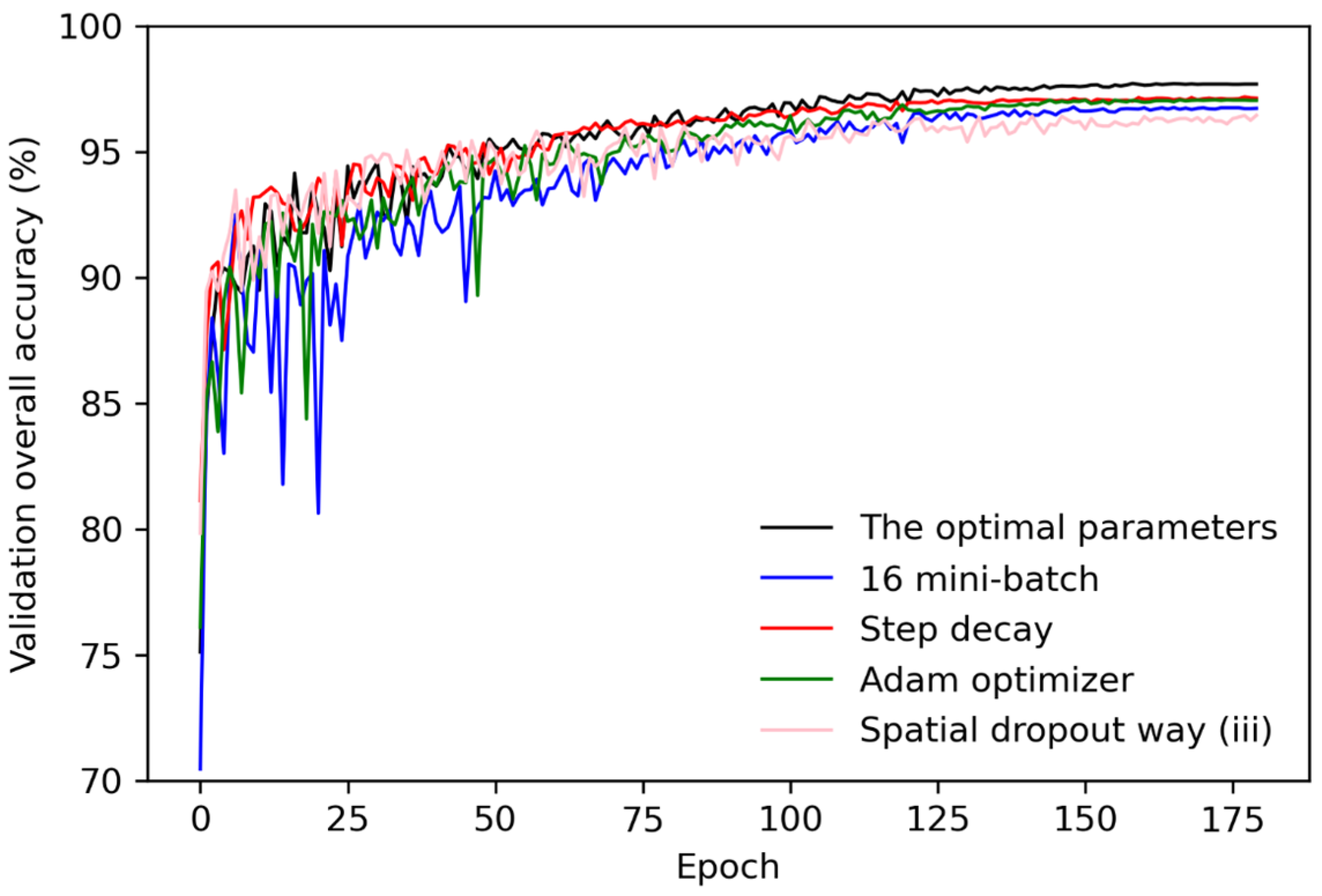
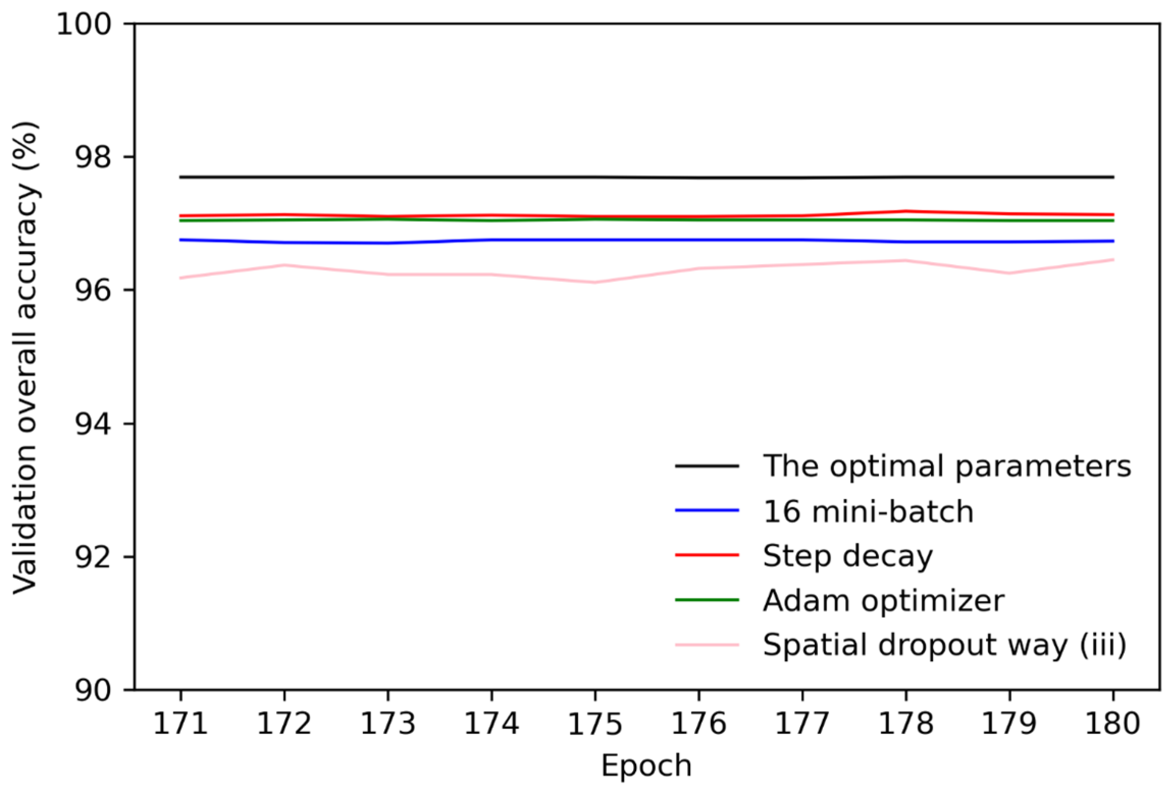
It is well established that deep learning results can vary considerably, regardless of the training data used, depending on the deep learning model structure and the parameterization [53,105]. The optimal LANA structure and parameterization presented in this study was found by undertaking a sensitivity analysis considering different feature map sizes and optimizers, as well as a range of learning rates, mini-batch sizes, and spatial dropout implementations. The final LANA structure used (Figure 3) was composed of 64, 128, 256, and 512 feature maps in four encoder convolution blocks (31,309,552 learnable coefficients) with an attention mechanism applied to the encoder feature maps when they were copied to the decoder side in the skip connections. The LANA was trained using 16,861 512 × 512 30 m pixel annotated patches, and the final implementation used a mini-batch size of 64 patches, a 0.0005 initial learning rate with a cosine learning rate decay strategy, the RMSProp optimizer algorithm, and spatial dropout applied to the last convolutional layer and to all the decoder layers before the transpose convolutions.

The LANA classification results were compared with the Fmask results available in the Landsat products and, in addition, with the results of the U-Net Wieland model that was developed and trained by [36]. The LANA classifies 30 m pixels into four classes (cloud, thin cloud, cloud shadow, and clear) and had a 77.91% overall classification accuracy, with class-specific accuracy increasing sequentially from thin cloud (F1-score 0.4104) to cloud shadow (0.5753), cloud (0.8139), and clear (0.8902) classes (Table 3). The very low F1-score of the thin cloud and shadow classes highlights the difficulty in detecting reliably thin clouds and cloud shadows due to the considerable spatial and spectral variability of these classes, which is evident in the 500 × 500 pixel subsets illustrated in Section 4.3.

The LANA, Fmask, and U-Net Wieland algorithms have different class legends, and, in order to provide meaningful intercomparison, the three algorithm classification results were harmonized to the same three classes, i.e., cloud, cloud shadow, and clear (Section 3.4). Considering the three classes, the LANA model had the highest (88.84%) overall accuracy, followed by Fmask (85.91%), and then U-Net Wieland (85.19%) (Table 4). The LANA had the highest F1-score accuracies for the three classes, which were >0.89 (clear), >0.91 (cloud), and >0.57 (cloud shadow). The Fmask and U-Net Wieland algorithm F1-score accuracies were lower for all three classes, particularly for cloud (Fmask 0.90, U-Net Wieland 0.88) and cloud shadow (Fmask 0.45, U-Net Wieland 0.52).

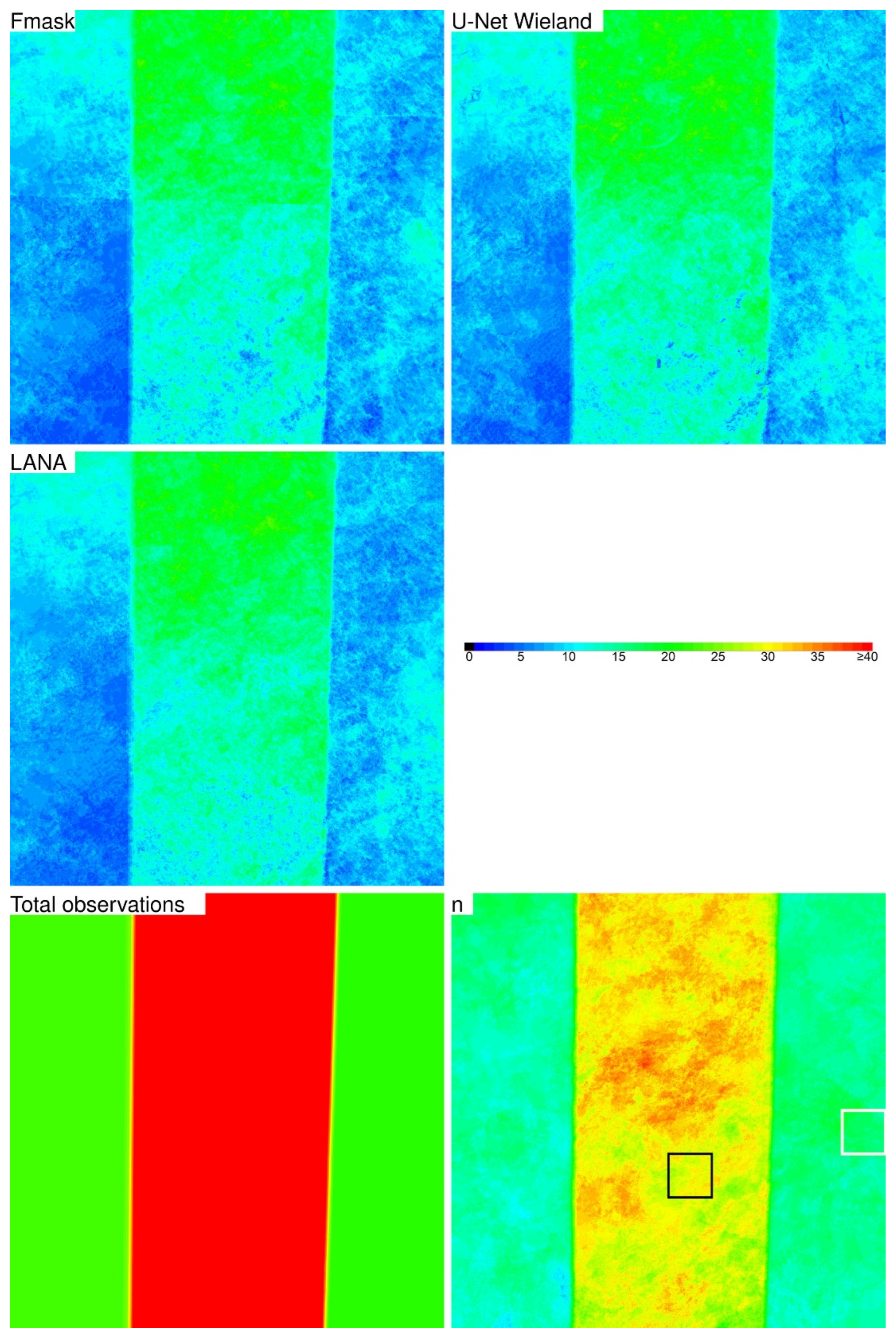
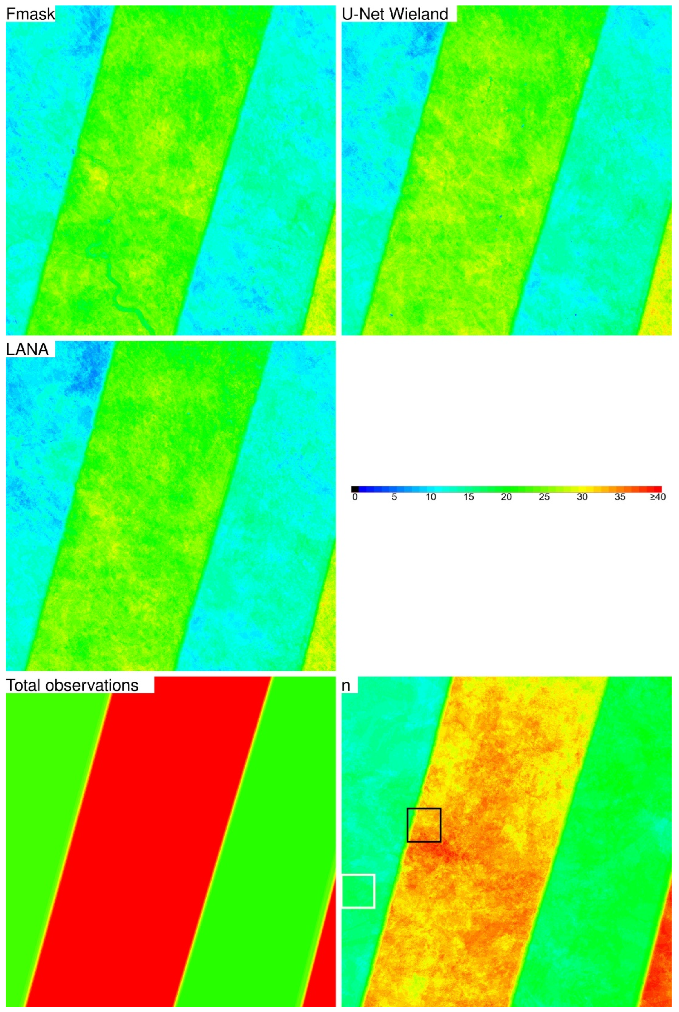
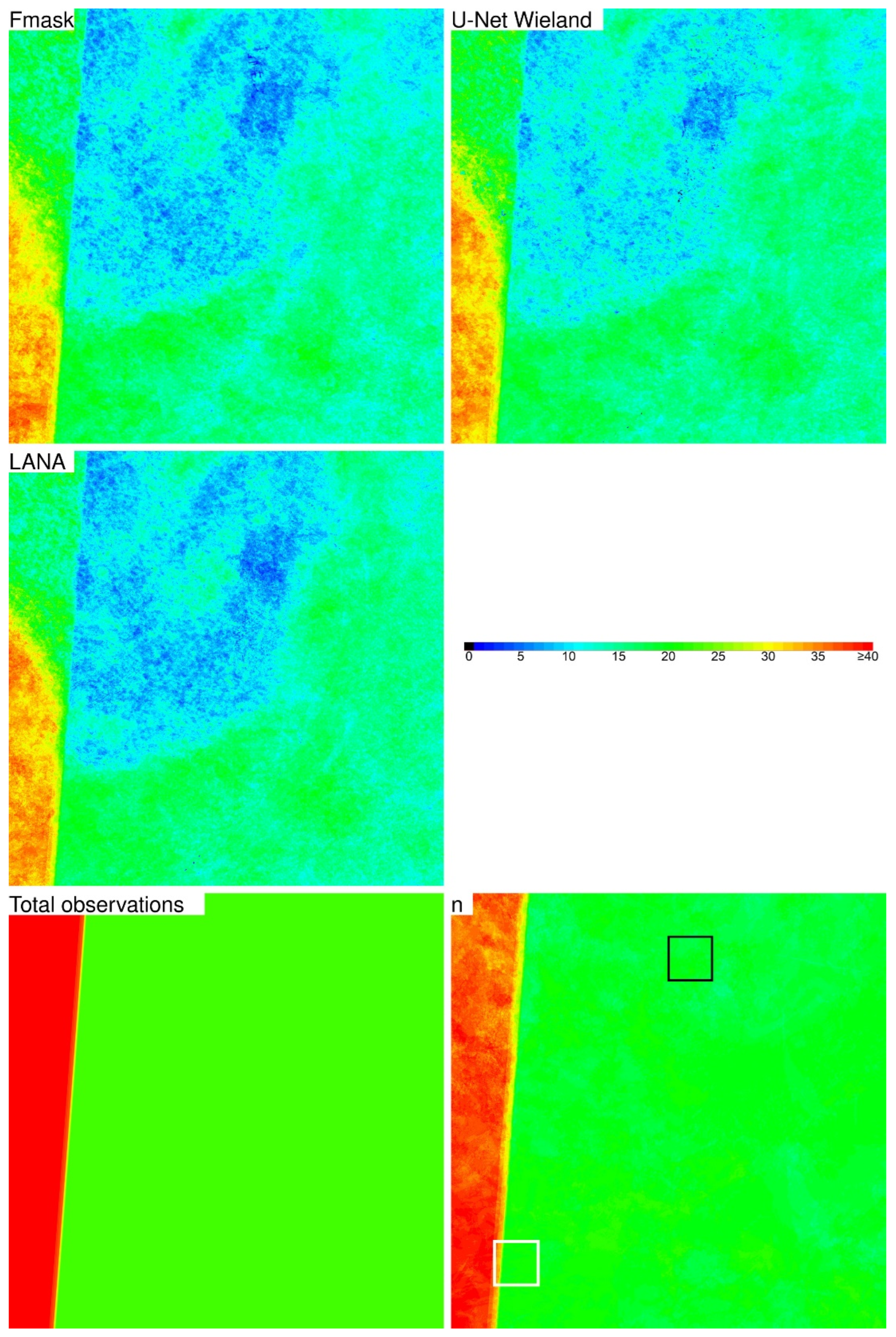
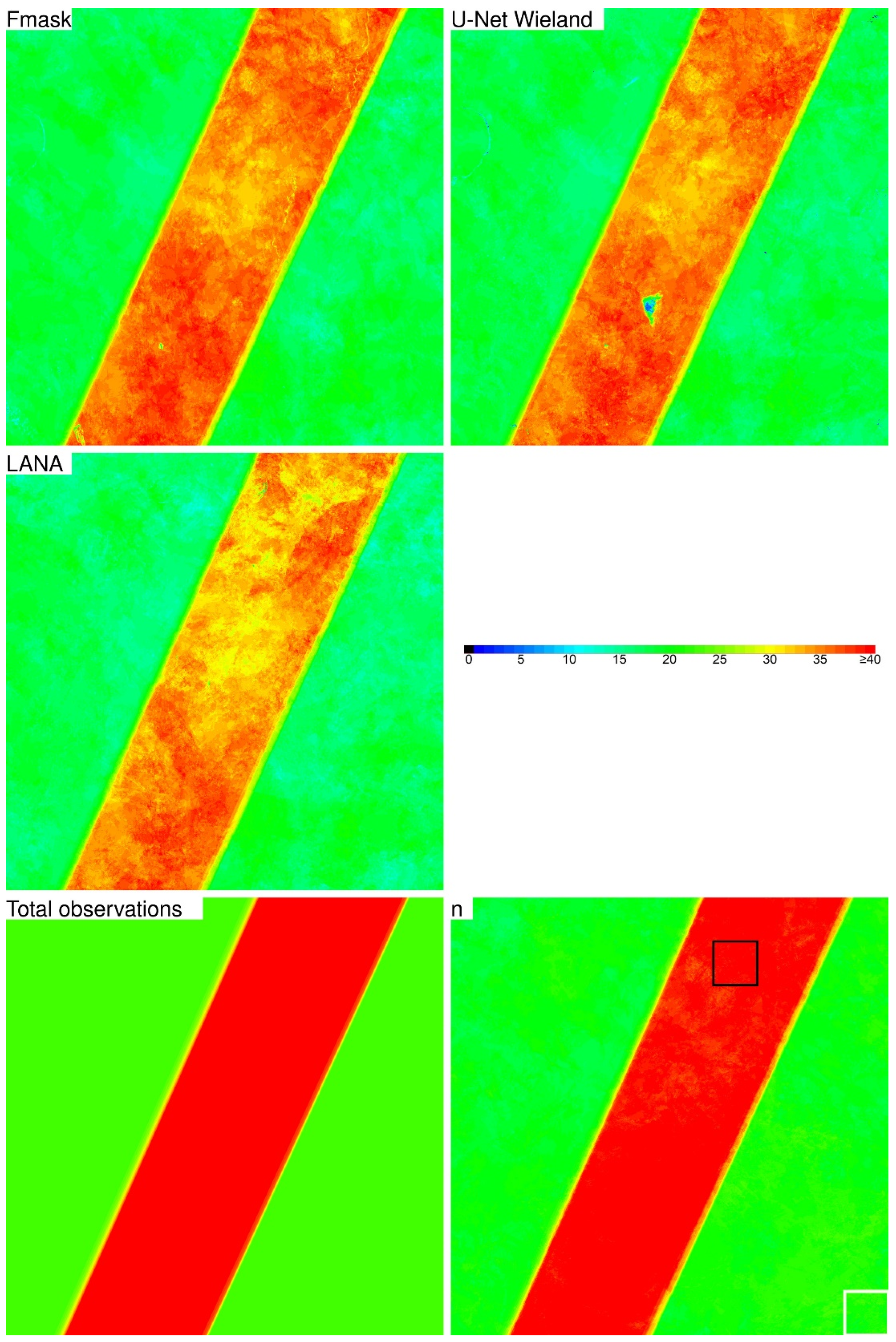
In addition to the accuracy assessment, a time-series evaluation was undertaken by applying each algorithm to a year of Collection 2 Landsat 8 OLI reflectance at four 5000 × 5000 30 m pixel CONUS ARD tiles. The ARD tiles encompassed different land surfaces and degrees of cloudiness and did not spatially coincide with the training data. At each ARD tile pixel, the temporal smoothness (TSI_λ) of the annual surface reflectance time series, considering only observations classified as “clear”, was quantified to provide insights into the prevalence of undetected clouds and cloud shadows, including sub-pixel clouds and shadows. The percentage of tile pixel observations classified as “clear” was similar for the three algorithms and so the algorithm TSI_λ values could be meaningfully compared. The LANA had the smallest tile-averaged TSI_λ values for 20 of the 24 (four tiles and six OLI bands/tile) TSI_λ comparisons, and the U-Net Wieland had marginally smaller values than the LANA for the remaining four comparisons. The Fmask had the greatest tile-averaged TSI_λ values for all bands for three of the ARD tiles, and for the other ARD tile (over Mexico/US that was the least cloudy), the Fmask had the greatest tile-averaged TSI_λ values for three of the six bands considered. The TSI_λ results indicate that the LANA had the lowest prevalence of undetected clouds and cloud shadows, whereas the Fmask had the greatest prevalence. This was also reflected in the class specific accuracy results. Among the three algorithms, the LANA had the smallest cloud and cloud shadow omission errors with 93.79% and 65.62% producer’s accuracies, respectively, whereas the Fmask had the greatest cloud omission error (86.57% producer’s accuracy) and the second greatest cloud shadow omission error (60.67% producer’s accuracy) (Table 3). The U-Net Wieland had the greatest cloud shadow omission error (50.88% producer’s accuracy). The U-Net Wieland had 89.31% cloud producer’s accuracy.

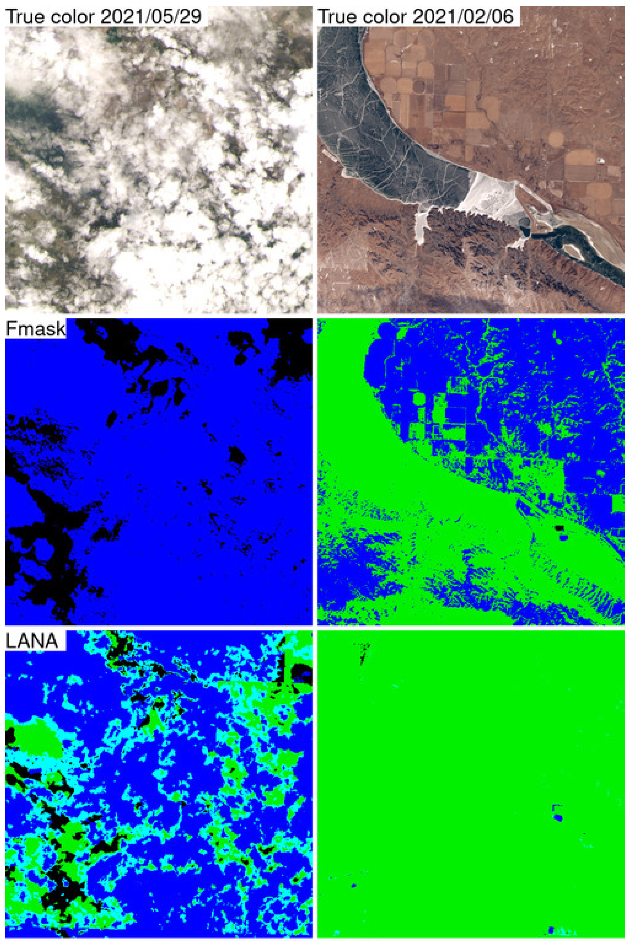
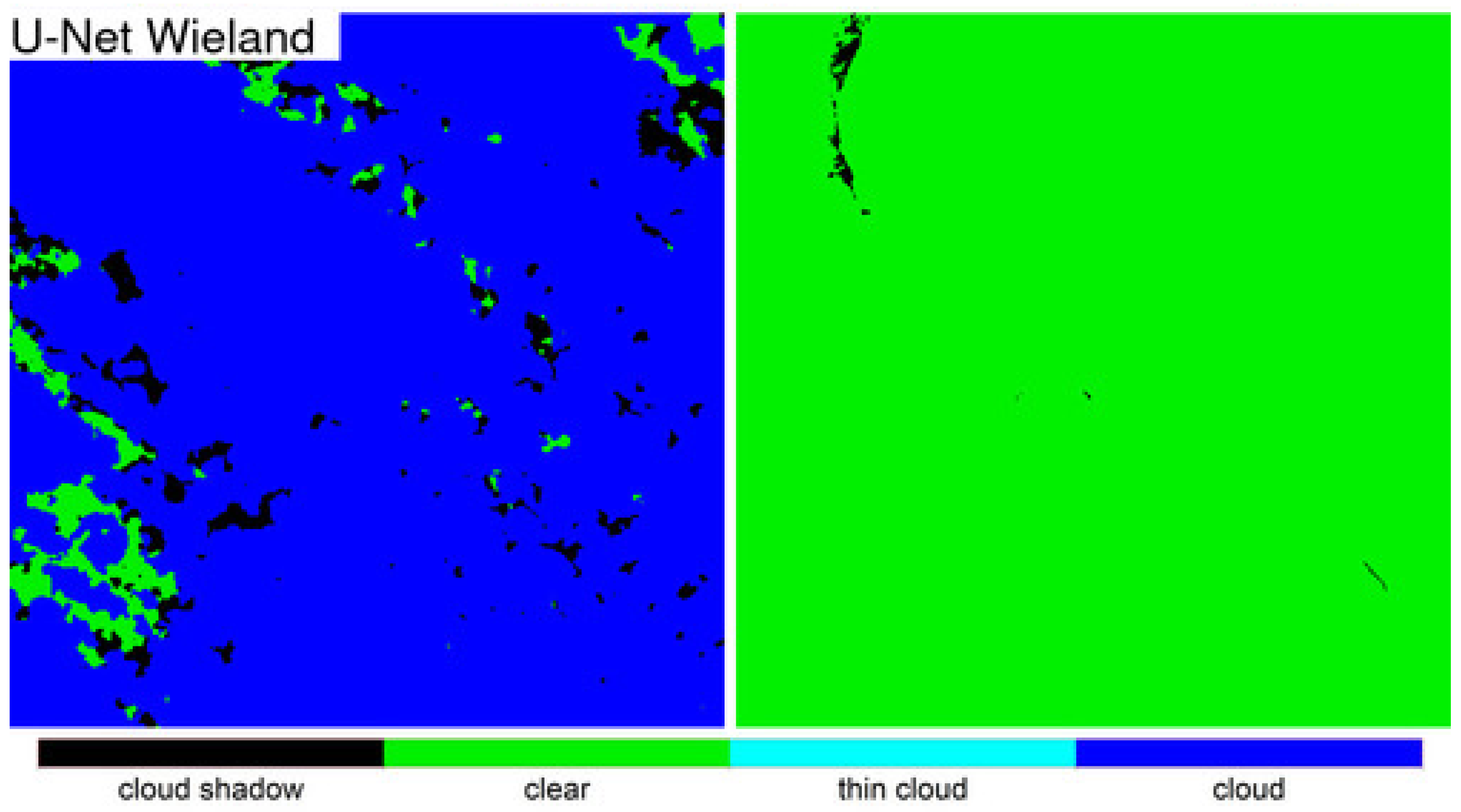
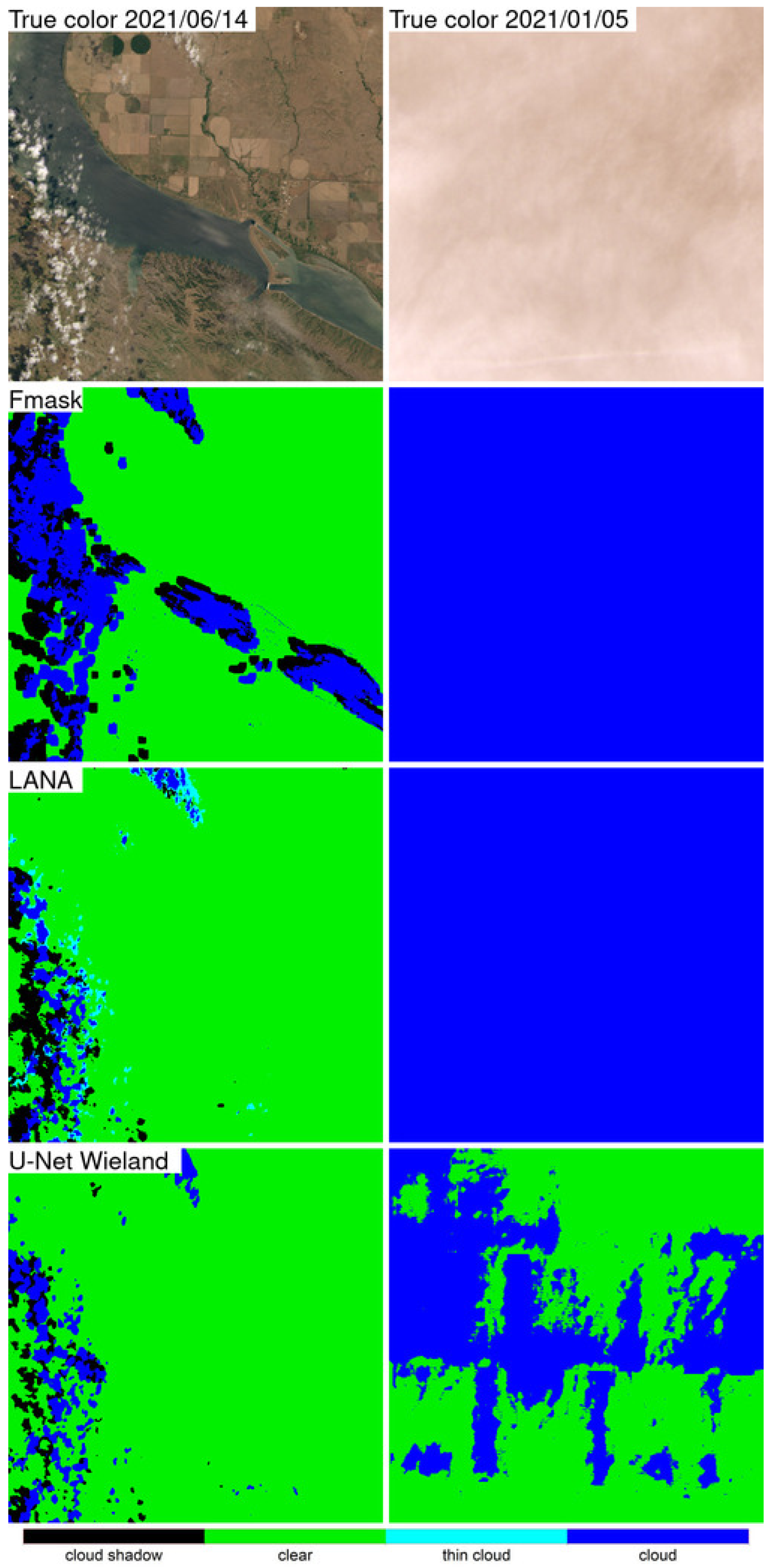
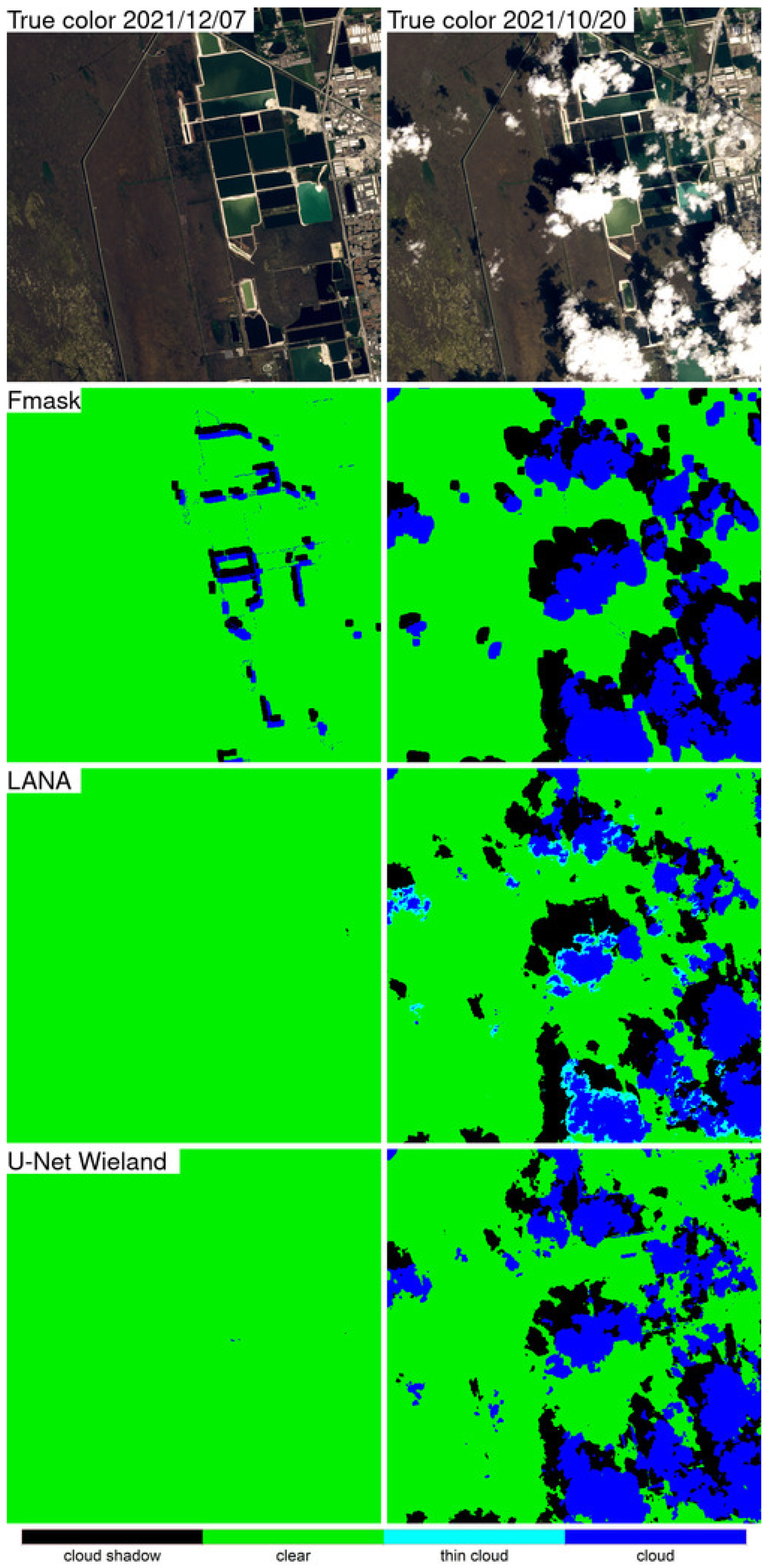
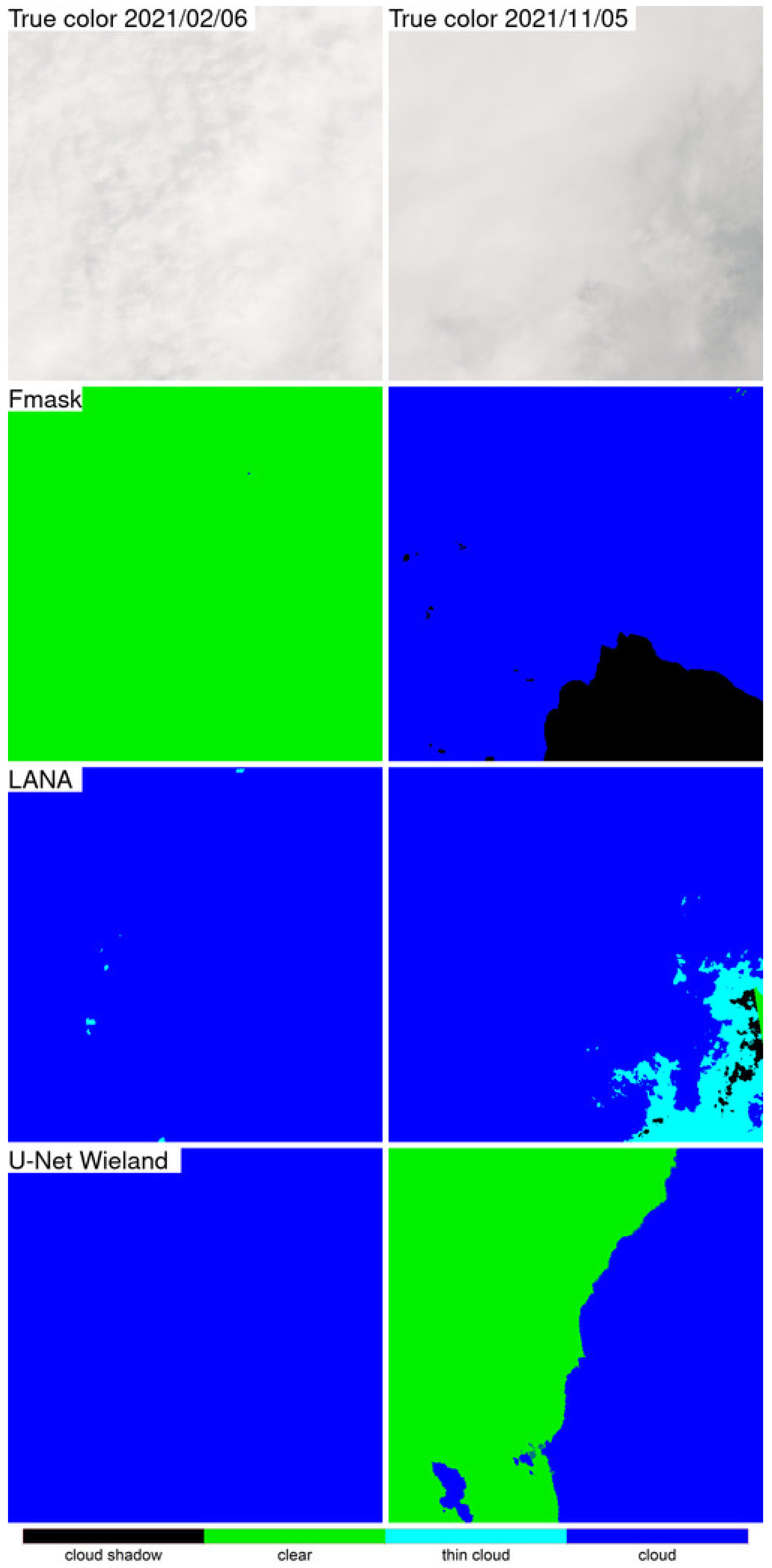
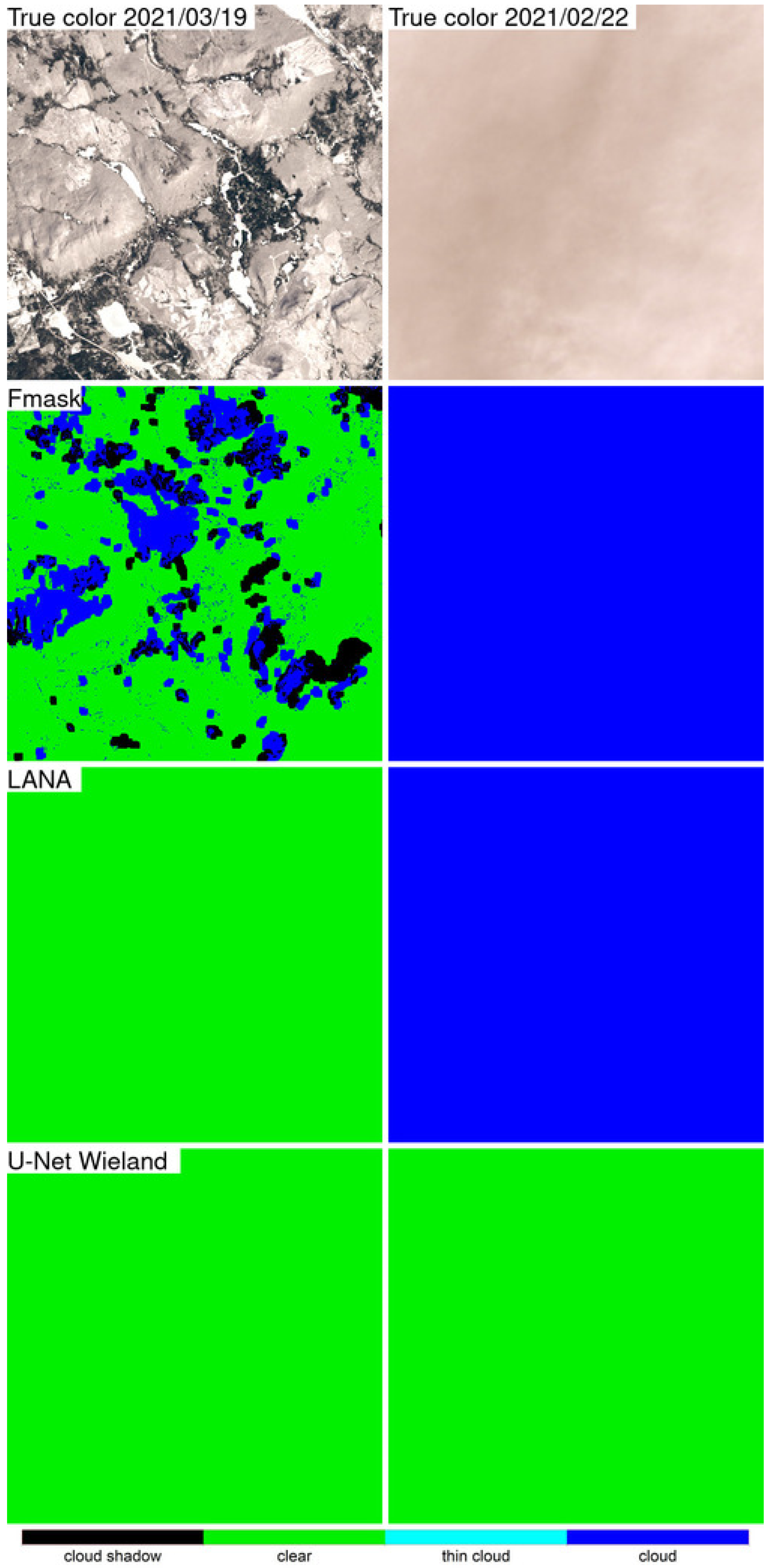
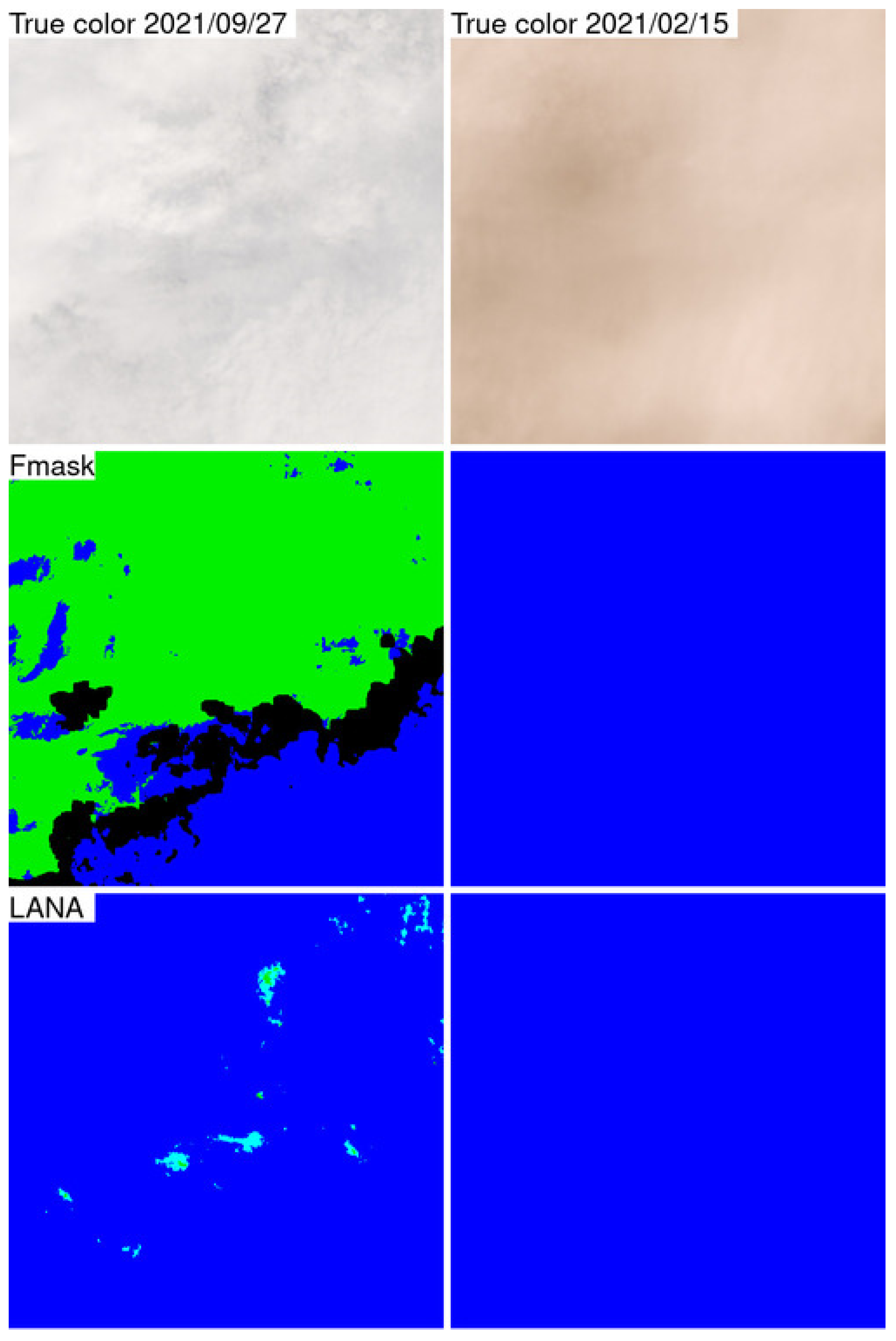
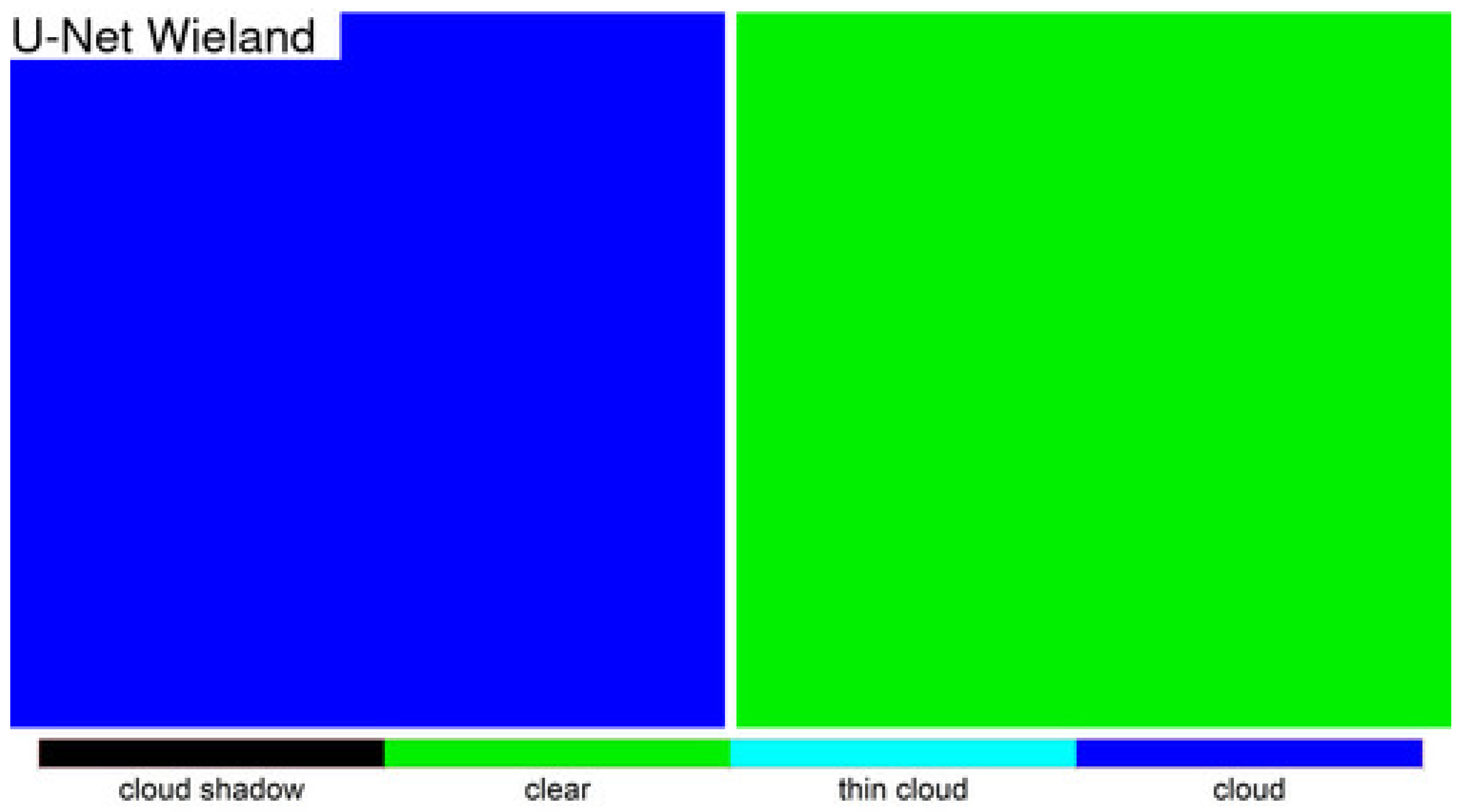
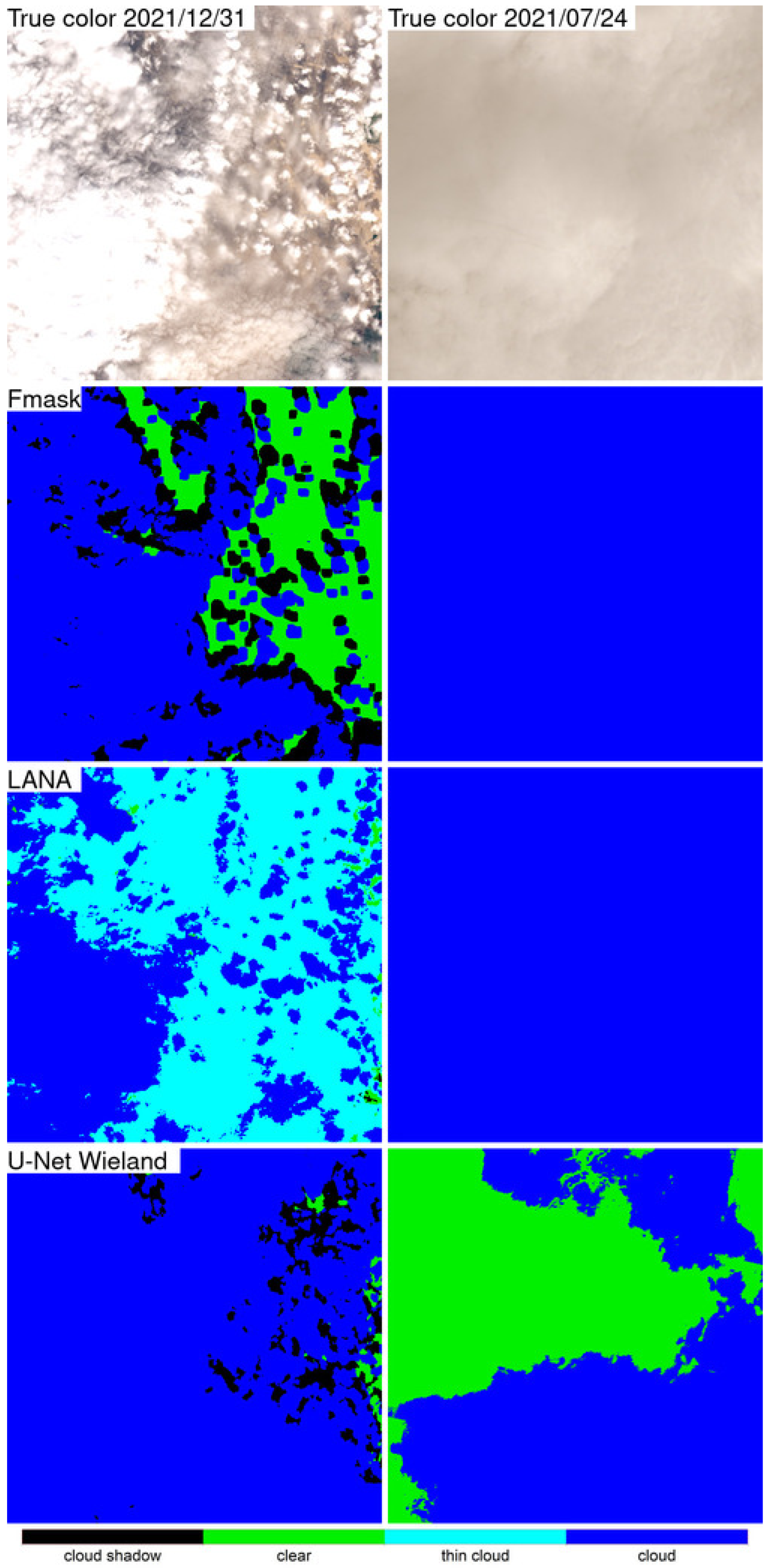
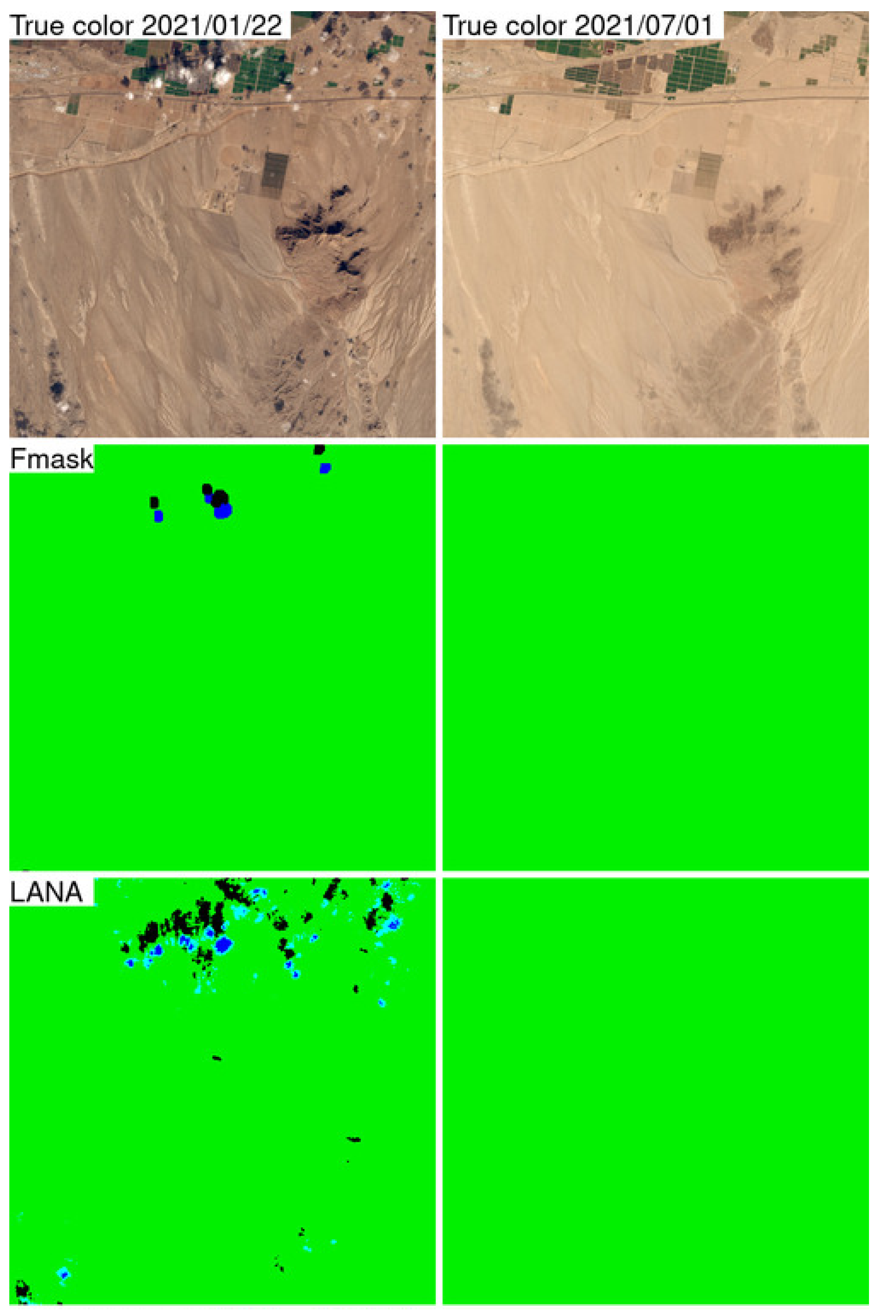
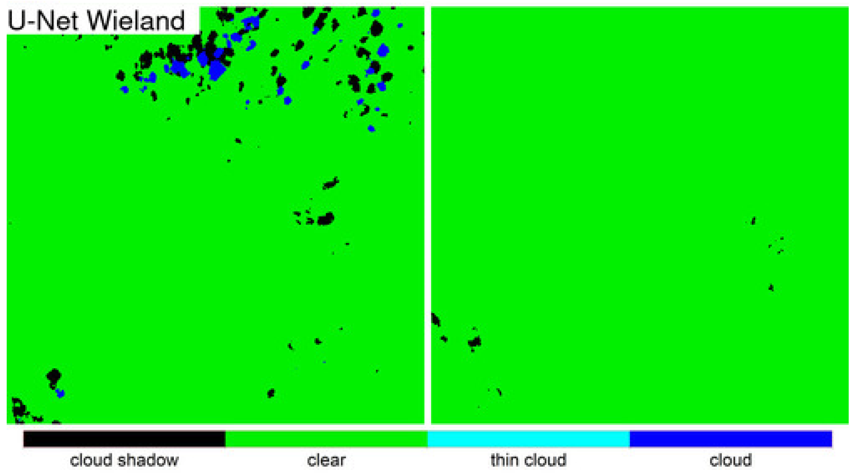
Detailed 500 × 500 30 m pixel ARD tile pixel subsets of the three algorithm classification results were compared qualitatively with the OLI reflectance for two dates selected based on the most different classification results between the LANA and each of the other two algorithms. The qualitative results were broadly consistent with the class specific accuracy assessment findings. The LANA algorithm typically performed better than Fmask and U-Net Wieland. Notably, the U-Net Wieland often failed to detect cloud and cloud shadows, and the Fmask occasionally missed obvious clouds and aggressively detected cloud shadows, which is reflected by it having the greatest cloud shadow commission error (36.30% user’s accuracy). These detailed visual assessments, and the ARD tile counts of annual “clear” observations, reinforce the need for cloud algorithm quality assessment. Formal accuracy assessment relies on a limited sample of validation data that may not adequately capture artefacts in the classification results, such as the Fmask stripe between successive Landsat images acquired in the same orbit and the U-Net Weiland cloud commission errors over bright desert, evident in Figure 9 and Figure 12, respectively.

The results presented in this study demonstrate that the LANA provides more reliable and accurate cloud and cloud shadow classification than the other algorithms. The Fmask and U-Net Wieland overall classification accuracies reported in this study are lower than those reported by the original algorithm publications. This is for several reasons. The U-Net Wieland authors reported a 91.0% accuracy for five classes (cloud shadow, cloud, water, land, and snow/ice), however, they used training and evaluation patches selected from the same images [36]. The Fmask Collection 1 overall accuracy was reported as 89.0% for three classes (cloud, cloud shadow, and clear) [21], and for Collection 2, it was reported as 85.1% [22]. The reported Fmask Collection 2 overall accuracy is close to the 85.91% Fmask accuracy reported in this study. Notably, however, we found that the 32 USGS annotated Landsat 8 OLI images used by [21] to validate the Collection 2 Fmask included images with missing cloud shadow annotations, and five images had visually indistinguishable cloud and snow areas that were unlikely to have been annotated perfectly. This underscores the need for high-quality annotation data that, ideally, should be derived at a higher resolution than the cloud/shadow results, as clouds and shadows occur at the sub-pixel level. International benchmarking and algorithm inter-comparison exercises, such as the Cloud Mask Intercomparison eXercise (CMIX) [106], are encouraged to generate annotated datasets that can be used for accuracy assessment and to investigate other ways of assessing cloud/shadow algorithms, although obtaining contemporaneous higher spatial resolution cloud/shadow information is challenging.

The LANA was implemented using the eight Landsat 8 OLI 30 m reflective bands and will also work for Landsat 9, which has the same reflective wavelength OLI bands and was launched successfully, after a short delay, in September 2021 [2]. The Landsat thermal bands were not used, even though clouds are often colder than land surfaces [107,108]. We found that including the two Landsat 8 thermal bands did not improve the LANA classification accuracy. This is likely because the emitted thermal radiance across a patch can vary rapidly due to factors, including the solar irradiance history, the surface type (e.g., specific heat capacity), wetness (rain and dew), and wind, which control latent and sensible heat fluxes. Further, cloud top temperatures can vary considerably, including with respect to cloud height, cloud optical depth, and ambient atmospheric temperature [109,110]. We also found that dropping the shorter wavelength OLI blue bands that are highly sensitive to aerosol scattering and that are difficult to reliably atmospherically correct [93,111] did not, like for other recent Landsat 8 OLI studies [67], significantly change the LANA classification accuracy.

Finally, we note that the LANA could be applied to other satellite sensors. The older Landsat sensor series have different spectral bands and spectral response functions [112], potentially complicating transfer learning approaches that have been developed for other Landsat deep learning applications [33,100]. In particular, the Landsat Multispectral Scanner (MSS) onboard Landsat 1–3 carried no blue or SWIR bands and had a coarser resolution [113,114], and research using the LANA for MSS cloud and cloud shadow masking is recommended. For reliable application to MSS, and to other sensor data, the LANA model should preferably be retrained. For example, the Sentinel-2 MultiSpectral Instrument (MSI) has similar but different spectral bands to the Landsat 8/9 OLI [115], and we note that Sentinel-2 cloud annotations are available [116,117], but no such datasets exist for MSS, and improved MSS cloud and cloud shadow masking is considered a future priority for the next Landsat collection [2].

References

1. Wulder, M.A.; Roy, D.P.; Radeloff, V.C.; Loveland, T.R.; Anderson, M.C.; Johnson, D.M.; Healey, S.; Zhu, Z.; Scambos, T.A.; Pahlevan, N.; et al. Fifty Years of Landsat Science and Impacts. Remote Sens. Environ. 2022, 280, 113195. [Google Scholar] [CrossRef]
2. Crawford, C.J.; Roy, D.P.; Arab, S.; Barnes, C.; Vermote, E.; Hulley, G.; Gerace, A.; Choate, M.; Engebretson, C.; Micijevic, E.; et al. The 50-Year Landsat Collection 2 Archive. Sci. Remote Sens. 2023, 8, 100103. [Google Scholar] [CrossRef]
3. Ackerman, S.A.; Strabala, K.I.; Menzel, W.P.; Frey, R.A.; Moeller, C.C.; Gumley, L.E. Discriminating Clear Sky from Clouds with MODIS. J. Geophys. Res. Atmos. 1998, 103, 32141–32157. [Google Scholar] [CrossRef]
4. Goodwin, N.R.; Collett, L.J.; Denham, R.J.; Flood, N.; Tindall, D. Cloud and Cloud Shadow Screening across Queensland, Australia: An Automated Method for Landsat TM/ETM+ Time Series. Remote Sens. Environ. 2013, 134, 50–65. [Google Scholar] [CrossRef]
5. Hollstein, A.; Segl, K.; Guanter, L.; Brell, M.; Enesco, M. Ready-to-Use Methods for the Detection of Clouds, Cirrus, Snow, Shadow, Water and Clear Sky Pixels in Sentinel-2 MSI Images. Remote Sens. 2016, 8, 666. [Google Scholar] [CrossRef]
6. Zhu, X.; Helmer, E.H. An Automatic Method for Screening Clouds and Cloud Shadows in Optical Satellite Image Time Series in Cloudy Regions. Remote Sens. Environ. 2018, 214, 135–153. [Google Scholar] [CrossRef]
7. Winker, D.M.; Pelon, J.R.; McCormick, M.P. The CALIPSO Mission: Spaceborne Lidar for Observation of Aerosols and Clouds. Lidar Remote Sens. Ind. Environ. Monit. III 2003, 4893, 1. [Google Scholar] [CrossRef]
8. Winker, D.M.; Vaughan, M.A.; Omar, A.; Hu, Y.; Powell, K.A.; Liu, Z.; Hunt, W.H.; Young, S.A. Overview of the CALIPSO Mission and CALIOP Data Processing Algorithms. J. Atmos. Ocean. Technol. 2009, 26, 2310–2323. [Google Scholar] [CrossRef]
9. Illingworth, A.J.; Barker, H.W.; Beljaars, A.; Ceccaldi, M.; Chepfer, H.; Clerbaux, N.; Cole, J.; Delanoë, J.; Domenech, C.; Donovan, D.P.; et al. The Earthcare Satellite: The next Step Forward in Global Measurements of Clouds, Aerosols, Precipitation, and Radiation. Bull. Am. Meteorol. Soc. 2015, 96, 1311–1332. [Google Scholar] [CrossRef]
10. Rossow, W.B.; Durden, S.L.; Miller, S.D.; Austin, R.T. THE CLOUDSAT MISSION AND THE A-TRAIN. Bull. Am. Meteorol. Soc. 2002, 83, 1771–1790. [Google Scholar]
11. Wang, J.; Rossow, W.B.; Zhang, Y. Cloud Vertical Structure and Its Variations from a 20-Yr Global Rawinsonde Dataset. J. Clim. 2000, 13, 3041–3056. [Google Scholar] [CrossRef]
12. Stubenrauch, C.J.; Chédin, A.; Rädel, G.; Scott, N.A.; Serrar, S. Cloud Properties and Their Seasonal Diurnal Variability from TOVS Path-B. J. Clim. 2006, 19, 5531–5533. [Google Scholar] [CrossRef]
13. Yuan, T.; Oreopoulos, L. On the Global Character of Overlap between Low and High Clouds. Geophys. Res. Lett. 2013, 40, 5320–5326. [Google Scholar] [CrossRef]
14. Lindquist, E.J.; Hansen, M.C.; Roy, D.P.; Justice, C.O. The Suitability of Decadal Image Data Sets for Mapping Tropical Forest Cover Change in the Democratic Republic of Congo: Implications for the Global Land Survey. Int. J. Remote Sens. 2008, 29, 7269–7275. [Google Scholar] [CrossRef]
15. Roy, D.P.; Ju, J.; Kline, K.; Scaramuzza, P.L.; Kovalskyy, V.; Hansen, M.; Loveland, T.R.; Vermote, E.; Zhang, C. Web-Enabled Landsat Data (WELD): Landsat ETM+ Composited Mosaics of the Conterminous United States. Remote Sens. Environ. 2010, 114, 35–49. [Google Scholar] [CrossRef]
16. Scaramuzza, P.L.; Bouchard, M.A.; Dwyer, J.L. Development of the Landsat Data Continuity Mission Cloud-Cover Assessment Algorithms. IEEE Trans. Geosci. Remote Sens. 2012, 50, 1140–1154. [Google Scholar] [CrossRef]
17. Hughes, M.J.; Hayes, D.J. Automated Detection of Cloud and Cloud Shadow in Single-Date Landsat Imagery Using Neural Networks and Spatial Post-Processing. Remote Sens. 2014, 6, 4907–4926. [Google Scholar] [CrossRef]
18. Ghasemian, N.; Akhoondzadeh, M. Introducing Two Random Forest Based Methods for Cloud Detection in Remote Sensing Images. Adv. Sp. Res. 2018, 62, 288–303. [Google Scholar] [CrossRef]
19. Wei, J.; Huang, W.; Li, Z.; Sun, L.; Zhu, X.; Yuan, Q.; Liu, L.; Cribb, M. Cloud Detection for Landsat Imagery by Combining the Random Forest and Superpixels Extracted via Energy-Driven Sampling Segmentation Approaches. Remote Sens. Environ. 2020, 248, 112005. [Google Scholar] [CrossRef]
20. Irish, R.R.; Barker, J.L.; Goward, S.N.; Arvidson, T. Characterization of the Landsat-7 ETM+ Automated Cloud-Cover Assessment (ACCA) Algorithm. Photogramm. Eng. Remote Sens. 2006, 72, 1179–1188. [Google Scholar] [CrossRef]
21. Zhu, Z.; Wang, S.; Woodcock, C.E. Improvement and Expansion of the Fmask Algorithm: Cloud, Cloud Shadow, and Snow Detection for Landsats 4–7, 8, and Sentinel 2 Images. Remote Sens. Environ. 2015, 159, 269–277. [Google Scholar] [CrossRef]
22. Foga, S.; Scaramuzza, P.L.; Guo, S.; Zhu, Z.; Dilley, R.D.; Beckmann, T.; Schmidt, G.L.; Dwyer, J.L.; Joseph Hughes, M.; Laue, B. Cloud Detection Algorithm Comparison and Validation for Operational Landsat Data Products. Remote Sens. Environ. 2017, 194, 379–390. [Google Scholar] [CrossRef]
23. Frantz, D.; Röder, A.; Stellmes, M.; Hill, J. An Operational Radiometric Landsat Preprocessing Framework for Large-Area Time Series Applications. IEEE Trans. Geosci. Remote Sens. 2016, 54, 3928–3943. [Google Scholar] [CrossRef]
24. Skakun, S.; Vermote, E.F.; Roger, J.C.; Justice, C.O.; Masek, J.G. Validation of the Lasrc Cloud Detection Algorithm for Landsat 8 Images. IEEE J. Sel. Top. Appl. Earth Obs. Remote Sens. 2019, 12, 2439–2446. [Google Scholar] [CrossRef]
25. Vermote, E.; Saleous, N. LEDAPS Surface Reflectance Product Description; University of Maryland: College Park, MD, USA, 2007; pp. 1–21. [Google Scholar]
26. Huang, N.; Niu, Z.; Wu, C.; Tappert, M.C. Modeling Net Primary Production of a Fast-Growing Forest Using a Light Use Efficiency Model. Ecol. Modell. 2010, 221, 2938–2948. [Google Scholar] [CrossRef]
27. Zhu, Z.; Woodcock, C.E. Object-Based Cloud and Cloud Shadow Detection in Landsat Imagery. Remote Sens. Environ. 2012, 118, 83–94. [Google Scholar] [CrossRef]
28. Sun, L.; Liu, X.; Yang, Y.; Chen, T.T.; Wang, Q.; Zhou, X. A Cloud Shadow Detection Method Combined with Cloud Height Iteration and Spectral Analysis for Landsat 8 OLI Data. ISPRS J. Photogramm. Remote Sens. 2018, 138, 193–207. [Google Scholar] [CrossRef]
29. Hagolle, O.; Huc, M.; Pascual, D.V.; Dedieu, G. A Multi-Temporal Method for Cloud Detection, Applied to FORMOSAT-2, VENμS, LANDSAT and SENTINEL-2 Images. Remote Sens. Environ. 2010, 114, 1747–1755. [Google Scholar] [CrossRef]
30. Xie, Y.; Li, Z.; Bao, H.; Jia, X.; Xu, D.; Zhou, X.; Skakun, S. Auto-CM: Unsupervised Deep Learning for Satellite Imagery Composition and Cloud Masking Using Spatio-Temporal Dynamics. In Proceedings of the 37th AAAI Conference on Artificial Intelligence, AAAI 2023, Philadelphia, PA, USA, 22–25 February 2023; Volume 37. [Google Scholar]
31. Long, J.; Shelhamer, E.; Darrell, T. Fully Convolutional Networks for Semantic Segmentation. In Proceedings of the IEEE Computer Society Conference on Computer Vision and Pattern Recognition, Washington, DC, USA, 7–12 June 2015; IEEE Computer Society: Washington, DC, USA, 14 October 2015; pp. 3431–3440. [Google Scholar]
32. Hughes, M.J.; Kennedy, R. High-Quality Cloud Masking of Landsat 8 Imagery Using Convolutional Neural Networks. Remote Sens. 2019, 11, 2591. [Google Scholar] [CrossRef]
33. Mateo-García, G.; Laparra, V.; López-Puigdollers, D.; Gómez-Chova, L. Transferring Deep Learning Models for Cloud Detection between Landsat-8 and Proba-V. ISPRS J. Photogramm. Remote Sens. 2020, 160, 1–17. [Google Scholar] [CrossRef]
34. Ronneberger, O.; Fischer, P.; Brox, T. U-Net: Convolutional Networks for Biomedical Image Segmentation. In Lecture Notes in Computer Science (Including Subseries Lecture Notes in Artificial Intelligence and Lecture Notes in Bioinformatics), Proceedings of the In Medical Image Computing and Computer-Assisted Intervention-MICCAI 2015: 18th International Conference, Munich, Germany, 5–9 October 2015; Springer: Berlin/Heidelberg, Germany, 2015; Volume 9351, pp. 234–241. [Google Scholar]
35. Zhang, Z.; Iwasaki, A.; Xu, G.; Song, J. Cloud Detection on Small Satellites Based on Lightweight U-Net and Image Compression. J. Appl. Remote Sens. 2019, 13, 1. [Google Scholar] [CrossRef]
36. Wieland, M.; Li, Y.; Martinis, S. Multi-Sensor Cloud and Cloud Shadow Segmentation with a Convolutional Neural Network. Remote Sens. Environ. 2019, 230, 111203. [Google Scholar] [CrossRef]
37. Hu, K.; Zhang, D.; Xia, M. Cdunet: Cloud Detection Unet for Remote Sensing Imagery. Remote Sens. 2021, 13, 4533. [Google Scholar] [CrossRef]
38. Jeppesen, J.H.; Jacobsen, R.H.; Inceoglu, F.; Toftegaard, T.S. A Cloud Detection Algorithm for Satellite Imagery Based on Deep Learning. Remote Sens. Environ. 2019, 229, 247–259. [Google Scholar] [CrossRef]
39. Chai, D.; Newsam, S.; Zhang, H.K.; Qiu, Y.; Huang, J. Cloud and Cloud Shadow Detection in Landsat Imagery Based on Deep Convolutional Neural Networks. Remote Sens. Environ. 2019, 225, 307–316. [Google Scholar] [CrossRef]
40. Yao, X.; Guo, Q.; Li, A. Light-Weight Cloud Detection Network for Optical Remote Sensing Images with Attention-Based DeeplabV3+ Architecture. Remote Sens. 2021, 13, 3617. [Google Scholar] [CrossRef]
41. Li, Z.; Shen, H.; Cheng, Q.; Liu, Y.; You, S.; He, Z. Deep Learning Based Cloud Detection for Medium and High Resolution Remote Sensing Images of Different Sensors. ISPRS J. Photogramm. Remote Sens. 2019, 150, 197–212. [Google Scholar] [CrossRef]
42. Mohajerani, S.; Saeedi, P. Cloud and Cloud Shadow Segmentation for Remote Sensing Imagery Via Filtered Jaccard Loss Function and Parametric Augmentation. IEEE J. Sel. Top. Appl. Earth Obs. Remote Sens. 2021, 14, 4254–4266. [Google Scholar] [CrossRef]
43. Luo, W.; Li, Y.; Urtasun, R.; Zemel, R. Understanding the Effective Receptive Field in Deep Convolutional Neural Networks. Adv. Neural Inf. Process. Syst. 2016, 29, 4905–4913. [Google Scholar]
44. Xu, K.; Ba, J.L.; Kiros, R.; Cho, K.; Courville, A.; Salakhutdinov, R.; Zemel, R.S.; Bengio, Y. Show, Attend and Tell: Neural Image Caption Generation with Visual Attention. In Proceedings of the 32nd International Conference on Machine Learning, ICML 2015, Lille, France, 6–11 July 2015; International Machine Learning Society (IMLS): Princeton, NJ, USA, 2015; Volume 3, pp. 2048–2057. [Google Scholar]
45. Zhang, H.; Goodfellow, I.; Metaxas, D.; Odena, A. Self-Attention Generative Adversarial Networks. In Proceedings of the 36th International Conference on Machine Learning, ICML 2019, Long Beach, CA, USA, 10–15 June 2019; International Machine Learning Society (IMLS): Princeton, NJ, USA, 2019; pp. 12744–12753. [Google Scholar]
46. Wang, X.; Girshick, R.; Gupta, A.; He, K. Non-Local Neural Networks. In Proceedings of the Proceedings of the IEEE Computer Society Conference on Computer Vision and Pattern Recognition, Salt Lake City, UT, USA, 14 December 2018; IEEE Computer Society: Washington, DC, USA, 2018; pp. 7794–7803. [Google Scholar]
47. Bahdanau, D.; Cho, K.H.; Bengio, Y. Neural Machine Translation by Jointly Learning to Align and Translate. In Proceedings of the 3rd International Conference on Learning Representations, ICLR 2015, San Diego, CA, USA, 7–9 May 2015. [Google Scholar]
48. Luong, M.T.; Pham, H.; Manning, C.D. Effective Approaches to Attention-Based Neural Machine Translation. In Proceedings of the Empirical Methods in Natural Language Processing Conference 2015, Lisbon, Portugal, 17–21 September 2015; pp. 1412–1421. [Google Scholar] [CrossRef]
49. Zhang, H.K.; Roy, D.P.; Kovalskyy, V. Optimal Solar Geometry Definition for Global Long-Term Landsat Time-Series Bidirectional Reflectance Normalization. IEEE Trans. Geosci. Remote Sens. 2016, 54, 1410–1418. [Google Scholar] [CrossRef]
50. Stumpf, A.; Kerle, N. Object-Oriented Mapping of Landslides Using Random Forests. Remote Sens. Environ. 2011, 115, 2564–2577. [Google Scholar] [CrossRef]
51. Waldner, F.; Chen, Y.; Lawes, R.; Hochman, Z. Needle in a Haystack: Mapping Rare and Infrequent Crops Using Satellite Imagery and Data Balancing Methods. Remote Sens. Environ. 2019, 233, 111375. [Google Scholar] [CrossRef]
52. Cloud Cover Assessment Validation Datasets. 2021. Available online: https://www.usgs.gov/landsat-missions/cloud-cover-assessment-validation-datasets (accessed on 1 August 2023).
53. Simonyan, K.; Zisserman, A. Very Deep Convolutional Networks for Large-Scale Image Recognition. In Proceedings of the 3rd International Conference on Learning Representations, ICLR 2015, San Diego, CA, USA, 7–9 May 2015. [Google Scholar]
54. He, K.; Zhang, X.; Ren, S.; Sun, J. Deep Residual Learning for Image Recognition. In Proceedings of the IEEE Computer Society Conference on Computer Vision and Pattern Recognition, Las Vegas, NV, USA, 9 December 2016; IEEE Computer Society: Washington, DC, USA, 2016; Volume 2016, pp. 770–778. [Google Scholar]
55. Dwyer, J.L.; Roy, D.P.; Sauer, B.; Jenkerson, C.B.; Zhang, H.K.; Lymburner, L. Analysis Ready Data: Enabling Analysis of the Landsat Archive. Remote Sens. 2018, 10, 1363. [Google Scholar] [CrossRef]
56. Roy, D.P.; Wulder, M.A.; Loveland, T.R.; Woodcock, C.E.; Allen, R.G.; Anderson, M.C.; Helder, D.; Irons, J.R.; Johnson, D.M.; Kennedy, R.; et al. Landsat-8: Science and Product Vision for Terrestrial Global Change Research. Remote Sens. Environ. 2014, 145, 154–172. [Google Scholar] [CrossRef]
57. Masek, J.G.; Wulder, M.A.; Markham, B.; McCorkel, J.; Crawford, C.J.; Storey, J.; Jenstrom, D.T. Landsat 9: Empowering Open Science and Applications through Continuity. Remote Sens. Environ. 2020, 248, 111968. [Google Scholar] [CrossRef]
58. USGS. Earth Resources Observation and Science (EROS) Center, Collection-2 Landsat 8-9 OLI (Operational Land Imager) and TIRS (Thermal Infrared Sensor) Level-1 Data Products; USGS: Garretson, SD, USA, 2022. [CrossRef]
59. Storey, J.; Roy, D.P.; Masek, J.; Gascon, F.; Dwyer, J.; Choate, M. A Note on the Temporary Misregistration of Landsat-8 Operational Land Imager (OLI) and Sentinel-2 Multi Spectral Instrument (MSI) Imagery. Remote Sens. Environ. 2016, 186, 121–122. [Google Scholar] [CrossRef]
60. Storey, J.C.; Rengarajan, R.; Choate, M.J. Bundle Adjustment Using Space-Based Triangulation Method for Improving the Landsat Global Ground Reference. Remote Sens. 2019, 11, 1640. [Google Scholar] [CrossRef]
61. Zhang, H.K.; Roy, D.P.; Luo, D. Demonstration of Large Area Land Cover Classification with a One Dimensional Convolutional Neural Network Applied to Single Pixel Temporal Metric Percentiles. Remote Sens. Environ. 2023, 295, 113653. [Google Scholar] [CrossRef]
62. Shorten, C.; Khoshgoftaar, T.M. A Survey on Image Data Augmentation for Deep Learning. J. Big Data 2019, 6, 60. [Google Scholar] [CrossRef]
63. Roy, D.P.; Zhang, H.K.; Ju, J.; Gomez-Dans, J.L.; Lewis, P.E.; Schaaf, C.B.; Sun, Q.; Li, J.; Huang, H.; Kovalskyy, V. A General Method to Normalize Landsat Reflectance Data to Nadir BRDF Adjusted Reflectance. Remote Sens. Environ. 2016, 176, 255–271. [Google Scholar] [CrossRef]
64. Ju, J.; Roy, D.P. The Availability of Cloud-Free Landsat ETM+ Data over the Conterminous United States and Globally. Remote Sens. Environ. 2008, 112, 1196–1211. [Google Scholar] [CrossRef]
65. Egorov, A.V.; Roy, D.P.; Zhang, H.K.; Li, Z.; Yan, L.; Huang, H. Landsat 4, 5 and 7 (1982 to 2017) Analysis Ready Data (ARD) Observation Coverage over the Conterminous United States and Implications for Terrestrial Monitoring. Remote Sens. 2019, 11, 447. [Google Scholar] [CrossRef]
66. Yan, L.; Roy, D.P. Spatially and Temporally Complete Landsat Reflectance Time Series Modelling: The Fill-and-Fit Approach. Remote Sens. Environ. 2020, 241, 111718. [Google Scholar] [CrossRef]
67. Zhai, Y.; Roy, D.P.; Martins, V.S.; Zhang, H.K.; Yan, L.; Li, Z. Conterminous United States Landsat-8 Top of Atmosphere and Surface Reflectance Tasseled Cap Transformation Coefficients. Remote Sens. Environ. 2022, 274, 112992. [Google Scholar] [CrossRef]
68. Tan, M.; Le, Q.V. EfficientNet: Rethinking Model Scaling for Convolutional Neural Networks. In Proceedings of the 36th International Conference on Machine Learning, ICML 2019; International Machine Learning Society (IMLS), Long Beach, CA, USA, 9–15 June 2019; Volume 2019, pp. 10691–10700. [Google Scholar]
69. Glorot, X.; Bordes, A.; Bengio, Y. Deep Sparse Rectifier Neural Networks. Proc. J. Mach. Learn. Res. 2011, 15, 315–323. [Google Scholar]
70. Peng, L.; Chen, X.; Chen, J.; Zhao, W.; Cao, X. Understanding the Role of Receptive Field of Convolutional Neural Network for Cloud Detection in Landsat 8 OLI Imagery. IEEE Trans. Geosci. Remote Sens. 2022, 60, 1–17. [Google Scholar] [CrossRef]
71. Dosovitskiy, A.; Beyer, L.; Kolesnikov, A.; Weissenborn, D.; Zhai, X.; Unterthiner, T.; Dehghani, M.; Minderer, M.; Heigold, G.; Gelly, S.; et al. An Image Is Worth 16X16 Words: Transformers for Image Recognition At Scale. In Proceedings of the 9rd International Conference on Learning Representations, ICLR 2021, Vienna, Austria, 3–7 May 2021. [Google Scholar]
72. Zhou, B.; Khosla, A.; Lapedriza, A.; Oliva, A.; Torralba, A. Object Detectors Emerge in Deep Scene CNNs. In Proceedings of the 3rd International Conference on Learning Representations, ICLR 2015, San Diego, CA, USA, 7–9 May 2015. [Google Scholar]
73. Yue, S.; Wang, T. Imbalanced Malware Images Classification: A CNN Based Approach. arXiv 2017, arXiv:1708.08042. [Google Scholar]
74. Kellenberger, B.; Marcos, D.; Tuia, D. Detecting Mammals in UAV Images: Best Practices to Address a Substantially Imbalanced Dataset with Deep Learning. Remote Sens. Environ. 2018, 216, 139–153. [Google Scholar] [CrossRef]
75. LeCun, Y.; Kanter, I.; Solla, S.A. Second Order Properties of Error Surfaces. Adv. Neural Inf. Process. Syst. 3 1990, 3, 918–924. [Google Scholar]
76. Abadi, M.; Agarwal, A.; Barham, P.; Brevdo, E.; Chen, Z.; Citro, C.; Corrado, G.S.; Davis, A.; Dean, J.; Devin, M.; et al. TensorFlow: Large-Scale Machine Learning on Heterogeneous Distributed Systems. arXiv 2016, arXiv:1603.04467. [Google Scholar]
77. Li, Y.; Chen, W.; Zhang, Y.; Tao, C.; Xiao, R.; Tan, Y. Accurate Cloud Detection in High-Resolution Remote Sensing Imagery by Weakly Supervised Deep Learning. Remote Sens. Environ. 2020, 250, 112045. [Google Scholar] [CrossRef]
78. Segal-Rozenhaimer, M.; Li, A.; Das, K.; Chirayath, V. Cloud Detection Algorithm for Multi-Modal Satellite Imagery Using Convolutional Neural-Networks (CNN). Remote Sens. Environ. 2020, 237, 111446. [Google Scholar] [CrossRef]
79. Xu, M.; Deng, F.; Jia, S.; Jia, X.; Plaza, A.J. Attention Mechanism-Based Generative Adversarial Networks for Cloud Removal in Landsat Images. Remote Sens. Environ. 2022, 271, 112902. [Google Scholar] [CrossRef]
80. Caraballo-Vega, J.A.; Carroll, M.L.; Neigh, C.S.R.; Wooten, M.; Lee, B.; Weis, A.; Aronne, M.; Alemu, W.G.; Williams, Z. Optimizing WorldView-2, -3 Cloud Masking Using Machine Learning Approaches. Remote Sens. Environ. 2023, 284, 113332. [Google Scholar] [CrossRef]
81. Smith, S.L.; Kindermans, P.J.; Ying, C.; Le, Q.V. Don’t Decay the Learning Rate, Increase the Batch Size. In Proceedings of the 6rd International Conference on Learning Representations, ICLR 2018, Vancouver, BC, Canada, 30 April—3 May 2018; pp. 1–11. [Google Scholar]
82. Ruder, S. An Overview of Gradient Descent Optimization Algorithms. arXiv 2016, arXiv:1609.04747. [Google Scholar]
83. Loshchilov, I.; Hutter, F. SGDR: Stochastic Gradient Descent with Warm Restarts. In Proceedings of the 5th International Conference on Learning Representations ICLR 2017, Conference Track Proceedings, Toulon, France, 24–26 April 2017; pp. 1–16. [Google Scholar]
84. Bao, H.; Dong, L.; Piao, S.; Wei, F. Beit: Bert Pre-Training of Image Transformers. In Proceedings of the ICLR 2022—10th International Conference on Learning Representations (ICLR), Virtual, 25–29 April 2022; pp. 1–18. [Google Scholar]
85. Liu, Z.; Mao, H.; Wu, C.-Y.; Feichtenhofer, C.; Darrell, T.; Xie, S. A convnet for the 2020s. In Proceedings of the IEEE/CVF Conference on Computer Vision and Pattern Recognition, New Orleans, LA, USA, 18–24 June 2022; pp. 11976–11986. [Google Scholar]
86. Kingma, D.P.; Ba, J.L. Adam: A Method for Stochastic Optimization. In Proceedings of the 3rd International Conference on Learning Representations, ICLR 2015, Conference Track Proceedings, San Diego, CA, USA, 7–9 May 2015; pp. 1–15. [Google Scholar]
87. Hinton, G.E.; Srivastava, N.; Krizhevsky, A.; Sutskever, I.; Salakhutdinov, R.R. Improving Neural Networks by Preventing Co-Adaptation of Feature Detectors. arXiv 2012, arXiv:1207.0580. [Google Scholar]
88. Tompson, J.; Goroshin, R.; Jain, A.; LeCun, Y.; Bregler, C. Efficient object localization using convolutional networks. In Proceedings of the IEEE Conference on Computer Vision and Pattern Recognition, Boston, MA, USA, 7–12 June 2015; pp. 648–656. [Google Scholar]
89. Shao, Z.; Pan, Y.; Diao, C.; Cai, J. Cloud Detection in Remote Sensing Images Based on Multiscale Features-Convolutional Neural Network. IEEE Trans. Geosci. Remote Sens. 2019, 57, 4062–4076. [Google Scholar] [CrossRef]
90. Houborg, R.; McCabe, M.F. Impacts of Dust Aerosol and Adjacency Effects on the Accuracy of Landsat 8 and RapidEye Surface Reflectances. Remote Sens. Environ. 2017, 194, 127–145. [Google Scholar] [CrossRef]
91. Tanre, D.; Herman, M.; Deschamps, P.Y. Influence of the Background Contribution upon Space Measurements of Ground Reflectance. Appl. Opt. 1981, 20, 3676. [Google Scholar] [CrossRef]
92. Ouaidrari, H.; Vermote, E.F. Operational Atmospheric Correction of Landsat TM Data. Remote Sens. Environ. 1999, 70, 4–15. [Google Scholar] [CrossRef]
93. Roy, D.P.; Qin, Y.; Kovalskyy, V.; Vermote, E.F.; Ju, J.; Egorov, A.; Hansen, M.C.; Kommareddy, I.; Yan, L. Conterminous United States Demonstration and Characterization of MODIS-Based Landsat ETM+ Atmospheric Correction. Remote Sens. Environ. 2014, 140, 433–449. [Google Scholar] [CrossRef]
94. Luo, Y.; Trishchenko, A.P.; Khlopenkov, K.V. Developing Clear-Sky, Cloud and Cloud Shadow Mask for Producing Clear-Sky Composites at 250-Meter Spatial Resolution for the Seven MODIS Land Bands over Canada and North America. Remote Sens. Environ. 2008, 112, 4167–4185. [Google Scholar] [CrossRef]
95. Hall, D.K.; Riggs, G.A. Mapping Global Snow Cover Using Moderate Resolution Imaging Spectroradiometer (MODIS) Data. Glaciol. Data 1995, 33, 13–17. [Google Scholar]
96. Salomonson, V.V.; Appel, I. Estimating Fractional Snow Cover from MODIS Using the Normalized Difference Snow Index. Remote Sens. Environ. 2004, 89, 351–360. [Google Scholar] [CrossRef]
97. Qiu, S.; Zhu, Z.; He, B. Fmask 4.0: Improved Cloud and Cloud Shadow Detection in Landsats 4–8 and Sentinel-2 Imagery. Remote Sens. Environ. 2019, 231, 111205. [Google Scholar] [CrossRef]
98. Franks, S.; Storey, J.; Rengarajan, R. The New Landsat Collection-2 Digital Elevation Model. Remote Sens. 2020, 12, 3909. [Google Scholar] [CrossRef]
99. Qiu, S.; Zhu, Z.; Woodcock, C.E. Cirrus Clouds That Adversely Affect Landsat 8 Images: What Are They and How to Detect Them? Remote Sens. Environ. 2020, 246, 111884. [Google Scholar] [CrossRef]
100. Martins, V.S.; Roy, D.P.; Huang, H.; Boschetti, L.; Zhang, H.K.; Yan, L. Deep Learning High Resolution Burned Area Mapping by Transfer Learning from Landsat-8 to PlanetScope. Remote Sens. Environ. 2022, 280, 113203. [Google Scholar] [CrossRef]
101. Russell, G. Congalton and Kass Green. Assessing the Accuracy of Remotely Sensed Data Principles and Practices, 3rd ed.; CRC Press: Boca Raton, FL, USA, 2019; Volume 1, ISBN 9788578110796. [Google Scholar]
102. Vermote, E.; Justice, C.O.; Bréon, F.M. Towards a Generalized Approach for Correction of the BRDF Effect in MODIS Directional Reflectances. IEEE Trans. Geosci. Remote Sens. 2009, 47, 898–908. [Google Scholar] [CrossRef]
103. Claverie, M.; Ju, J.; Masek, J.G.; Dungan, J.L.; Vermote, E.F.; Roger, J.C.; Skakun, S.V.; Justice, C. The Harmonized Landsat and Sentinel-2 Surface Reflectance Data Set. Remote Sens. Environ. 2018, 219, 145–161. [Google Scholar] [CrossRef]
104. Huang, H.; Roy, D.P. Characterization of Planetscope-0 Planetscope-1 Surface Reflectance and Normalized Difference Vegetation Index Continuity. Sci. Remote Sens. 2021, 3, 100014. [Google Scholar] [CrossRef]
105. Krizhevsky, A.; Sutskever, I.; Hinton, G.E. ImageNet Classification with Deep Convolutional Neural Networks. In Proceedings of the Advances in Neural Information Processing Systems, Lake Tahoe, NV, USA, 3–8 December 2012; Volume 2, pp. 1097–1105. [Google Scholar]
106. Skakun, S.; Wevers, J.; Brockmann, C.; Doxani, G.; Aleksandrov, M.; Batič, M.; Frantz, D.; Gascon, F.; Gómez-Chova, L.; Hagolle, O.; et al. Cloud Mask Intercomparison EXercise (CMIX): An Evaluation of Cloud Masking Algorithms for Landsat 8 and Sentinel-2. Remote Sens. Environ. 2022, 274, 112990. [Google Scholar] [CrossRef]
107. Hulley, G.C.; Hook, S.J. A New Methodology for Cloud Detection and Classification with ASTER Data. Geophys. Res. Lett. 2008, 35, 1–6. [Google Scholar] [CrossRef]
108. Weng, Q.; Fu, P. Modeling Annual Parameters of Clear-Sky Land Surface Temperature Variations and Evaluating the Impact of Cloud Cover Using Time Series of Landsat TIR Data. Remote Sens. Environ. 2014, 140, 267–278. [Google Scholar] [CrossRef]
109. Marchand, R.; Ackerman, T.; Smyth, M.; Rossow, W.B. A Review of Cloud Top Height and Optical Depth Histograms from MISR, ISCCP, and MODIS. J. Geophys. Res. Atmos. 2010, 115, 1–25. [Google Scholar] [CrossRef]
110. Tselioudis, G.; Rossow, W.B.; Rind, D. Global Patterns of Cloud Optical Thickness Variation with Temperature. J. Clim. 1992, 5, 1484–1495. [Google Scholar] [CrossRef]
111. Doxani, G.; Vermote, E.; Roger, J.C.; Gascon, F.; Adriaensen, S.; Frantz, D.; Hagolle, O.; Hollstein, A.; Kirches, G.; Li, F.; et al. Atmospheric Correction Inter-Comparison Exercise. Remote Sens. 2018, 10, 352. [Google Scholar] [CrossRef] [PubMed]
112. Roy, D.P.; Kovalskyy, V.; Zhang, H.K.; Vermote, E.F.; Yan, L.; Kumar, S.S.; Egorov, A. Characterization of Landsat-7 to Landsat-8 Reflective Wavelength and Normalized Difference Vegetation Index Continuity. Remote Sens. Environ. 2016, 185, 57–70. [Google Scholar] [CrossRef]
113. Markham, B.L.; Barker, J.L. Radiometric properties of US processed Landsat MSS data. Remote Sens. Environ. 1987, 22, 39–71. [Google Scholar] [CrossRef]
114. Braaten, J.D.; Cohen, W.B.; Yang, Z. Automated Cloud and Cloud Shadow Identification in Landsat MSS Imagery for Temperate Ecosystems. Remote Sens. Environ. 2015, 169, 128–138. [Google Scholar] [CrossRef]
115. Drusch, M.; Del Bello, U.; Carlier, S.; Colin, O.; Fernandez, V.; Gascon, F.; Hoersch, B.; Isola, C.; Laberinti, P.; Martimort, P.; et al. Sentinel-2: ESA’s Optical High-Resolution Mission for GMES Operational Services. Remote Sens. Environ. 2012, 120, 25–36. [Google Scholar] [CrossRef]
116. Tarrio, K.; Tang, X.; Masek, J.G.; Claverie, M.; Ju, J.; Qiu, S.; Zhu, Z.; Woodcock, C.E. Comparison of Cloud Detection Algorithms for Sentinel-2 Imagery. Sci. Remote Sens. 2020, 2, 100010. [Google Scholar] [CrossRef]
117. Li, J.; Wu, Z.; Sheng, Q.; Wang, B.; Hu, Z.; Zheng, S.; Camps-Valls, G.; Molinier, M. A Hybrid Generative Adversarial Network for Weakly-Supervised Cloud Detection in Multispectral Images. Remote Sens. Environ. 2022, 280, 113197. [Google Scholar] [CrossRef] [PubMed]
118. Yang, J.; Guo, J.; Yue, H.; Liu, Z.; Hu, H.; Li, K. CDnet: CNN-Based Cloud Detection for Remote Sensing Imagery. IEEE Trans. Geosci. Remote Sens. 2019, 57, 6195–6211. [Google Scholar] [CrossRef]
119. Francis, A.; Sidiropoulos, P.; Muller, J.P. CloudFCN: Accurate and Robust Cloud Detection for Satellite Imagery with Deep Learning. Remote Sens. 2019, 11, 2312. [Google Scholar] [CrossRef]
120. Yin, Z.; Ling, F.; Foody, G.M.; Li, X.; Du, Y. Cloud Detection in Landsat-8 Imagery in Google Earth Engine Based on a Deep Convolutional Neural Network. Remote Sens. Lett. 2020, 11, 1181–1190. [Google Scholar] [CrossRef]
121. Jiao, L.; Huo, L.; Hu, C.; Tang, P. Refined UNet: UNet-Based Refinement Network for Cloud and Shadow Precise Segmentation. Remote Sens. 2020, 12, 2001. [Google Scholar] [CrossRef]
122. Guo, Y.; Cao, X.; Liu, B.; Gao, M. Cloud Detection for Satellite Imagery Using Attention-Based U-Net Convolutional Neural Network. Symmetry 2020, 12, 1056. [Google Scholar] [CrossRef]
123. Guo, H.; Bai, H.; Qin, W. ClouDet: A Dilated Separable CNN-Based Cloud Detection Framework for Remote Sensing Imagery. IEEE J. Sel. Top. Appl. Earth Obs. Remote Sens. 2021, 14, 9743–9755. [Google Scholar] [CrossRef]
124. López-Puigdollers, D.; Mateo-García, G.; Gómez-Chova, L. Benchmarking Deep Learning Models for Cloud Detection in Landsat-8 and Sentinel-2 Images. Remote Sens. 2021, 13, 992. [Google Scholar] [CrossRef]
125. Wang, W.; Shi, Z. An All-Scale Feature Fusion Network with Boundary Point Prediction for Cloud Detection. IEEE Geosci. Remote Sens. Lett. 2022, 19, 3110869. [Google Scholar] [CrossRef]
126. Zhang, G.; Gao, X.; Yang, Y.; Wang, M.; Ran, S. Controllably Deep Supervision and Multi-Scale Feature Fusion Network for Cloud and Snow Detection Based on Medium-and High-Resolution Imagery Dataset. Remote Sens. 2021, 13, 4805. [Google Scholar] [CrossRef]
127. Hu, K.; Zhang, D.; Xia, M.; Qian, M.; Chen, B. LCDNet: Light-Weighted Cloud Detection Network for High-Resolution Remote Sensing Images. IEEE J. Sel. Top. Appl. Earth Obs. Remote Sens. 2022, 15, 4809–4823. [Google Scholar] [CrossRef]
128. Lu, C.; Xia, M.; Qian, M.; Chen, B. Dual-Branch Network for Cloud and Cloud Shadow Segmentation. IEEE Trans. Geosci. Remote Sens. 2022, 60, 3175613. [Google Scholar] [CrossRef]
129. Francis, A.M.; Mrziglod, J.; Sidiropoulos, P.; Muller, J.P. SEnSeI: A Deep Learning Module for Creating Sensor Independent Cloud Masks. IEEE Trans. Geosci. Remote Sens. 2022, 60, 3128280. [Google Scholar] [CrossRef]
130. Zhang, L.; Sun, J.; Yang, X.; Jiang, R.; Ye, Q. Improving Deep Learning-Based Cloud Detection for Satellite Images with Attention Mechanism. IEEE Geosci. Remote Sens. Lett. 2022, 19, 3133872. [Google Scholar] [CrossRef]
131. Guo, Q.; Tong, L.; Yao, X.; Wu, Y.; Wan, G. CD_HIEFNet: Cloud Detection Network Using Haze Optimized Transformation Index and Edge Feature for Optical Remote Sensing Imagery. Remote Sens. 2022, 14, 14153701. [Google Scholar] [CrossRef]
132. Li, X.; Yang, X.; Li, X.; Lu, S.; Ye, Y.; Ban, Y. GCDB-UNet: A Novel Robust Cloud Detection Approach for Remote Sensing Images. Knowl.-Based Syst. 2022, 238, 107890. [Google Scholar] [CrossRef]
133. Kaur Buttar, P.; Sachan, M.K. Semantic Segmentation of Clouds in Satellite Images Based on U-Net++ Architecture and Attention Mechanism. Expert Syst. Appl. 2022, 209, 118380. [Google Scholar] [CrossRef]
134. Ma, N.; Sun, L.; He, Y.; Zhou, C.; Dong, C. CNN-TransNet: A Hybrid CNN-Transformer Network with Differential Feature Enhancement for Cloud Detection. IEEE Geosci. Remote Sens. Lett. 2023, 20, 3288742. [Google Scholar] [CrossRef]
135. Pang, S.; Sun, L.; Tian, Y.; Ma, Y.; Wei, J. Convolutional Neural Network-Driven Improvements in Global Cloud Detection for Landsat 8 and Transfer Learning on Sentinel-2 Imagery. Remote Sens. 2023, 15, 1706. [Google Scholar] [CrossRef]
136. Yao, X.; Guo, Q.; Li, A. Cloud Detection in Optical Remote Sensing Images with Deep Semi-Supervised and Active Learning. IEEE Geosci. Remote Sens. Lett. 2023, 20, 3287537. [Google Scholar] [CrossRef]
137. Chen, K.; Dai, X.; Xia, M.; Weng, L.; Hu, K.; Lin, H. MSFANet: Multi-Scale Strip Feature Attention Network for Cloud and Cloud Shadow Segmentation. Remote Sens. 2023, 15, 4853. [Google Scholar] [CrossRef]
138. Gong, C.; Long, T.; Yin, R.; Jiao, W.; Wang, G. A Hybrid Algorithm with Swin Transformer and Convolution for Cloud Detection. Remote Sens. 2023, 15, 5264. [Google Scholar] [CrossRef]
139. Li, K.; Ma, N.; Sun, L. Cloud Detection of Multi-Type Satellite Images Based on Spectral Assimilation and Deep Learning. Int. J. Remote Sens. 2023, 44, 3106–3121. [Google Scholar] [CrossRef]
140. Chen, Y.; Tang, L.; Huang, W.; Guo, J.; Yang, G. A Novel Spectral Indices-Driven Spectral-Spatial-Context Attention Network for Automatic Cloud Detection. IEEE J. Sel. Top. Appl. Earth Obs. Remote Sens. 2023, 16, 3092–3103. [Google Scholar] [CrossRef]
Figure 1. Distribution of the annotated USGS images, SPARCS image subsets and SDSU images, each composed of Collection 1 Landsat 8 OLI 30 m TOA reflectance bands and corresponding 30 m annotations (cloud, thin cloud, cloud shadow, or clear). The USGS and SDSU images cover ~185 × 180 km (typically 6200 × 6000 30 m pixels) and the SPARCS subsets cover 1000 × 1000 30 m pixels. The circled USGS images show the five set aside annotated USGS Landsat 8 OLI evaluation images used for accuracy assessment (Section 3.5). The locations of the Collection 2 ARD 5000 × 5000 30 m pixel tiles are also shown (see Section 2.4).
Remotesensing 16 01321 g001
Figure 2. The four 5000 × 5000 30 m pixel ARD tiles used in the time-series analysis (a) tile h28v04 (Canada/US), (b) tile h05v13 (Mexico/US), (c) tile h15v06 (South Dakota), (d) tile h27v19 (Florida). The median of the cloud-free red, green, blue (true color) Landsat 8 TOA reflectance sensed from 1 May to 30 September 2021 (with Fmask labeled clouds and cloud shadows masked out) is illustrated. The colored boxes show 500 × 500 30 m subsets selected for detailed visual examination that are illustrated in Section 4.
Remotesensing 16 01321 g002
Figure 3. The LANA structure used to classify 512 × 512 30 m pixel patches with eight Landsat 8 spectral bands into four classes: cloud, thin cloud, cloud shadow, and clear. The horizontal gray arrows show skip connections used to copy feature maps from the encoder (light gray rectangles) to their decoder block counterpart. The black curved arrows show the attention mechanism interactions.
Remotesensing 16 01321 g003
Figure 4. The overall accuracy of the 4% validation dataset as a function of training epoch ((top): Epochs 1–180; (bottom) epochs: 171–180) for different training parameters using the LANA (64) structure (shown in Figure 3). The black line shows the optimal parameter set results (see text) and the colored lines show the results for parameter combinations where one parameter was different to the optimal set.
Remotesensing 16 01321 g004aRemotesensing 16 01321 g004b
Figure 5. The annual number of Landsat 8 OLI non-cirrus and non-saturated observations flagged as “clear” from 1 January to 31 December 2021 by the three algorithms at each 5000 × 5000 30 m ARD pixel of the Florida tile (h28v04, illustrated in Figure 2d). The bottom row shows the annual number of Landsat 8 OLI observations, regardless of the cirrus or saturation state, and the annual number of non-cirrus and non-saturated (n) observations at each ARD pixel. The white and black squares show 500 × 500 30 m pixel subsets (also shown in Figure 2d), for which algorithm classification results are illustrated in Figure 6 and Figure 7.
Remotesensing 16 01321 g005
Figure 6. Two dates (columns) of the Fmask, LANA, and U-Net Wieland classification results (rows) for a 500 × 500 30 m pixel Florida tile subset over land (subset boundary shown black in Figure 2d and Figure 5). The top row shows the true color (red, green, blue) 30 m reflectance for context. The left and right columns show the dates in 2021 with the most different classification results between LANA and Fmask, and between LANA and U-Net Wieland, respectively. The LANA algorithm results are shown colored as cloud (dark blue), thin cloud (light blue), cloud shadow (black), and clear (green). The Fmask and U-Net Wieland results harmonized to three classes are shown similarly colored as cloud (dark blue), cloud shadow (black), and clear (green).
Remotesensing 16 01321 g006
Figure 7. As Figure 6 but for a 500 × 500 30 m pixel Florida tile subset over water (subset boundary show white in Figure 2d and Figure 5).
Remotesensing 16 01321 g007
Figure 8. The annual number of Landsat 8 OLI non-cirrus and non-saturated observations flagged as “clear” from 1 January to 31 December 2021 by the three algorithms at each 5000 × 5000 30 m ARD pixel of the Canada/US tile (h28v04, illustrated in Figure 2a). The bottom row shows the annual number of Landsat 8 OLI observations, regardless of the cirrus or saturation state, and the annual number of non-cirrus and non-saturated (n) observations at each ARD pixel. The white and black squares show 500 × 500 30 m pixel subsets (also shown in Figure 2a), for which algorithm classification results are illustrated in Figure 9 and Figure 10.
Remotesensing 16 01321 g008
Figure 9. Two dates (columns) of the Fmask, LANA, and U-Net Wieland classification results (rows) for a 500 × 500 30 m pixel Canada/US tile subset over forest (subset boundary shown black in Figure 2a and Figure 7). The top row shows the true color (red, green, blue) 30 m reflectance for context. The left and right columns show the dates in 2021 with the most different classification results between LANA and Fmask, and between LANA and U-Net Wieland, respectively. The LANA algorithm results are shown colored as cloud (dark blue), thin cloud (light blue), cloud shadow (black), and clear (green). The Fmask and U-Net Wieland results harmonized to three classes are shown similarly colored as cloud (dark blue), cloud shadow (black), and clear (green).
Remotesensing 16 01321 g009
Figure 10. As Figure 9 but for a 500 × 500 30 m pixel Canada/US tile subset over a water and cropland mixed area (subset boundary shown in white in Figure 2a and Figure 8).
Remotesensing 16 01321 g010aRemotesensing 16 01321 g010b
Figure 11. The annual number of Landsat 8 OLI non-cirrus and non-saturated observations flagged as “clear” from 1 January to 31 December 2021 by the three algorithms at each 5000 × 5000 30 m ARD pixel of the Mexico/US tile (h05v13, illustrated in Figure 2b). The bottom row shows the annual number of Landsat 8 OLI observations, regardless of the cirrus or saturation state, and the annual number of non-cirrus and non-saturated (n) observations at each ARD pixel. The white and black squares show 500 × 500 30 m pixel subsets (also shown in Figure 2b), for which algorithm classification results are illustrated in Figure 12 and Figure 13.
Remotesensing 16 01321 g011
Figure 12. Two dates (columns) of the Fmask, LANA, and U-Net Wieland classification results (rows) for a 500 × 500 30 m pixel Mexico/US tile subset over desert (subset boundary shown in black in Figure 2b and Figure 10). The top row shows the true color (red, green, blue) 30 m reflectance for context. The left and right columns show the dates in 2021 with the most different classification results between LANA and Fmask, and between LANA and U-Net Wieland, respectively. The LANA algorithm results are shown colored as cloud (dark blue), thin cloud (light blue), cloud shadow (black), and clear (green). The Fmask and U-Net Wieland results harmonized to three classes are shown similarly colored as cloud (dark blue), cloud shadow (black), and clear (green).
Remotesensing 16 01321 g012
Figure 13. As Figure 12 but for a 500 × 500 30 m pixel Mexico/US tile subset over a desert and cropland mixed area (subset boundary shown in white in Figure 2b and Figure 10).
Remotesensing 16 01321 g013aRemotesensing 16 01321 g013b
Figure 14. The annual number of Landsat 8 OLI non-cirrus and non-saturated observations flagged as “clear” from 1 January to 31 December 2021 by the three algorithms at each 5000 × 5000 30 m ARD pixel of the South Dakota tile (h15v06, illustrated in Figure 2c). The bottom row shows the annual number of Landsat 8 OLI observations, regardless of the cirrus or saturation state, and the annual number of non-cirrus and non-saturated (n) observations at each ARD pixel. The white and black squares show 500 × 500 30 m pixel subsets (also shown in Figure 2c), for which algorithm classification results are illustrated in Figure 15 and Figure 16.
Remotesensing 16 01321 g014
Figure 15. As Figure 15, but for a 500 × 500 30 m pixel South Dakota tile subset over a cropland area (subset boundary shown in white in Figure 2c and Figure 14).
Remotesensing 16 01321 g015aRemotesensing 16 01321 g015b
Figure 16. Two dates (columns) of the Fmask, LANA, and U-Net Wieland classifications results (rows) for a 500 × 500 30 m pixel South Dakota tile subset over Missouri River (subset boundary shown in black in Figure 2c and Figure 14). The top row shows the true color (red, green, blue) 30 m reflectance for context. The left and right columns show the dates in 2021 with the most different classification results between LANA and Fmask, and between LANA and U-Net Wieland, respectively. The LANA algorithm results are shown colored as cloud (dark blue), thin cloud (light blue), cloud shadow (black), and clear (green). The Fmask and U-Net Wieland results harmonized to three classes are shown similarly colored as cloud (dark blue), cloud shadow (black), and clear (green).
Remotesensing 16 01321 g016