Article

Mapping Dissolved Organic Carbon and Organic Iron by Comparing Deep Learning and Linear Regression Techniques Using Sentinel-2 and WorldView-2 Imagery (Byers Peninsula, Maritime Antarctica)

by
Susana del Carmen Fernández
1,*,
Rubén Muñiz
2,
Juanjo Peón
3,
Ricardo Rodríguez-Cielos
4,
Jesús Ruíz
5 and
Javier F. Calleja
6
1
Department of Geology and ICTEA (Instituto Universitario de Ciencias y Tecnologías Aeroespaciales de Asturias), University of Oviedo, 33003 Oviedo, Spain
2
Department of Computer Science, University of Oviedo, 33003 Oviedo, Spain
3
Department of Mining Exploitation and Prospecting, University of Oviedo, 33600 Mieres, Spain
4
Department of Signals, Systems and Radiocommunications (SSR), Polytechnic University of Madrid, 28040 Madrid, Spain
5
Department of Geography, University of Oviedo, 33003 Oviedo, Spain
6
Department of Physics, University of Oviedo, 33003 Oviedo, Spain
*
Author to whom correspondence should be addressed.
Remote Sens. 2024, 16(7), 1192; https://doi.org/10.3390/rs16071192
Submission received: 25 February 2024 / Revised: 23 March 2024 / Accepted: 25 March 2024 / Published: 28 March 2024
(This article belongs to the Special Issue GIS and Remote Sensing in Soil Mapping and Modeling)

Abstract

:
Byers Peninsula is considered one of the largest ice-free areas in maritime Antarctica. Since 2006, the Spanish Polar Program has taken part in a large number of environmental studies involving the effects of climate change on biological life cycles, limnology, and microbiology. Soils from maritime Antarctica are generally weakly developed and have chemical, physical, and morphological characteristics that are strongly influenced by the parent material. However, biological activity during the short Antarctic summer promotes intense transference of nutrients and organic matter in areas occupied by different species of birds and marine mammals. Mapping and monitoring those areas that are highly occupied by various species could be very useful to create models prepared from satellite images of the edaphic properties. In this approach, deep learning and linear regression models of the soil properties and spectral indexes, which were considered as explicative variables, were used. We trained the models on soil properties closely related to biological activity such as dissolved organic carbon (DOC) and the iron fraction associated with the organic matter (Fe). We tested the best approach to model the spatial distribution of DOC, Fe, and pH by training the linear regression and deep learning models on Sentinel-2 and WorldView-2 images. The most robust models, the pH model built with the deep learning approach on Sentinel images (MAE of 0.51, RMSE of 0.70, and R2 with a residual of −0.49), the DOC model built with linear regression on Sentinel images (MAE of 189.39, RMSE of 342.23, and R2 with a residual of 0.0), and the organic Fe model built with deep learning (MAE of 116.20, RMSE of 209.93, and R2 of −0.05), were used to track possible areas with ornithogenic soils, as well as areas of Byers Peninsula that could be supporting the highest biological development.

1. Introduction

Byers Peninsula is located at the eastern end of Livingston Island in a maritime Antarctic environment that comprises part of the Antarctic Peninsula and the surrounding islands (Figure 1). Byers Peninsula with a surface area of about 60 km2 is considered one of the largest ice-free areas in maritime Antarctica and is an Antarctic Special Protected Area (ASPA No. 126), redesignated as a Site of Special Scientific Interest (SSSI). The primary reason for the designation of Byers Peninsula as an ASPA and SSSI is to protect the terrestrial and lacustrine habitats within the area. The reasons for this protection include the diversity of plant and animal life [1], the many invertebrates, a population of southern elephant seals (Mirounga leonina), small colonies of Antarctic fur seals (Arctocephalus gazella), and a large variety of plants and animals within a relatively small area [2]. During the fourth International Polar Year, Byers Peninsula was established as an ‘International Antarctic Reference Site for Terrestrial, Freshwater, and Coastal Ecosystems’. Predicting the ecological variations after large-scale climate change has been the main goal of research projects such as LIMNOPOLAR [3]. During this period, baseline data on terrestrial, limnic, and coastal ecosystems were collected, including the characteristics of the permafrost [4], the geomorphology and geochemistry [5,6], vegetation extent [7], the limnic diversity and function [3,8], the marine mammal and bird diversity [9], the microbiology [10], and the diversity of coastal marine invertebrates. Refs. [11,12] provide a review of all scientific work published in this field between 1957 and 2012.
Despite the remoteness of this part of Antarctica and the adverse working conditions, information on soil formation in the area is relatively abundant (see [13,14,15,16] and the references therein). The soil survey of the ice-free Byers Peninsula suggests that mosses are the main cause of the organic soils and were found throughout the ice-free areas of maritime Antarctica in association with mineral soils [14]. Nevertheless, intense penguin activity on the ice-free areas along the Antarctic coast leads to the formation of ornithogenic soils [13,17,18]. According to [17], the accumulation of guano in penguin rookeries is the most abundant source of organic matter in the terrestrial ecosystem of Antarctica. Skuas (Catharacta sp.) and other flying birds that nest around penguin rookeries also extend the ornithogenic influence [17].
At upland sites on Byers Peninsula with no vegetation or ornithogenic influence, the soil chemistry and mineralogy are related mainly to the physical weathering of the substrata [19]. However, the ornithogenic influence alters the soil’s characteristics, leading to soil acidification, the leaching of exchangeable bases, the transformation of primary minerals, and the release of amorphous Fe and Al [16]. The ornithogenic soils are readily distinguishable from the non-ornithogenic soils by lower pH and higher organic matter values [14,20].
Apart from the ornithogenic origin of the organic matter in Byers Peninsula’s soils, the results of the study by [21] showed that the colonization of the substrate by plants is associated with a higher rate of mineral weathering, which has clear repercussions for the mobility and bioavailability of many elements. That study found higher amounts of labile organic matter (DOC) and Fe in soils with vegetation compared to non-vegetated soils. Although Byers Peninsula is almost free of vegetation, from an Antarctic point of view, the vegetation is relatively rich along the more low-lying coastal areas, especially on the South Beaches and President Beaches. At these sites, vegetation is favored by a more advantageous local climate and by nutrient supplies from marine mammals and birds [17]. Deschanylsia antarctica and Colobanthus quitensis, the flowering plants of Antarctica, can be found in the low-lying areas of Byers Peninsula, along with mosses, lichens, liverworts, and fungi. Extensive carpets of mosses along the President and South Beaches are dominated by Dreparwcladus uncinatus. The progressive colonization of this part of Byers Peninsula by plants may accelerate edaphogenesis, while also substantially affecting the mobility and bioavailability of macronutrients and micronutrients [21]. Sodium pyrophosphate-extracted Fe in Byers Peninsula’s soils can be considered as the fraction bound to organic matter (organochelates) and used to estimate the mobility of organo-iron complexes [22]. Thus, accelerated mineral weathering by plants and microorganisms may increase the bioavailable forms of Fe in coastal and lacustrine waters in the medium and long term.
Conducting field surveys in Byers Peninsula poses significant difficulties due to extreme environmental conditions, in addition to the completely restricted access. However, there are numerous works on digital mapping of the Antarctic environment based on satellite remote sensing data [23,24,25,26,27]. Images are used as soil predictors, assuming that remote sensing data can provide detailed information on soil properties [28]. This assumption is better applied in areas without continuous vegetation cover, as is the case in Antarctica. Ref. [29] used Sentinel-2 spectral indexes as predictor variables to make soil texture maps of all bare soils in maritime Antarctica.
In this work, we trained models of soil properties closely related to biological activity, such as dissolved organic carbon (DOC) and the iron fraction associated with organic matter (Fe) or chelated iron and, also, pH. We tested the best approach to model the spatial distribution of these key soil properties by training linear regression (LRM) and deep learning neural network (DL) models over Sentinel-2 and WorldView-2 imagery. The most robust models were used to track possible areas of ornithogenic soils and areas of Byers Peninsula that could support the highest biological development.
The objectives of this research were the following:
  • To train models of soil properties using optical satellite imagery such as Sentinel-2 and WordView2.
  • To search for spectral indices that could be useful for tracking dissolved organic carbon and iron chelates in Byers Peninsula as a training plot for maritime Antarctic periglacial areas.
  • To look for the areas most likely to be biologically colonized. These areas, if accessible, should be the main target of exhaustive inventories and analyses to elucidate the true causes of the increase in their indicators of biological activity.

2. Materials and Methods

2.1. Byers Peninsula

Byers Peninsula (Figure 1) is located at the western end of Livingston Island, South Shetland Islands (approximately 62° 13 70 S, 61° 1 60 W), where environmental conditions are more favorable for soil development than in other Antarctic regions [14,21]). This peninsula is a site of special biogeochemical and ecological interest [3]. Biodiversity at this site is higher than at other nearby sites, possibly due to mild environmental conditions, the proximity to South America, and possible wind transport of propagules [30].

2.1.1. Geology and Geomorphology

Glaciers cover most of Livingstone Island, except for Byers Peninsula, which is the largest ice-free area in the South Shetland Islands. The chronology of the deglaciation process has been determined from the dating of deeper lake sediments [31]. The last major deglaciation of the peninsula occurred 5–4 ka BP [32]. The geological substrates of the peninsula are mainly sandstones, shales, microconglomerates, and volcanic and volcaniclastic rocks (Upper Jurassic to Lower Cretaceous) with igneous bodies [31,33,34]. Except for the northwestern part of the peninsula, which reaches 268 m.a.s.l., few areas reach elevations above 100 m.a.s.l., except for a few remnant hills (usually volcanic plugs). The highest of these, Chester Cone, forms a prominent feature in the central part of the peninsula, 193 m high. The inland part of the peninsula is a regular undivided platform of about 40 km2 and between 85 and 100 m high, the “Byers Plateau” [35,36], and most of the peninsula is surrounded by extensive beaches.

2.1.2. Climate, Weathering, and Soils

The average annual precipitation in the region can exceed 800 mm, and the average annual temperature is about –2.8 °C. In summer, mean temperatures are above freezing. The region shows moderate winds throughout the year, and with moderate, mostly liquid precipitation during the summer, precipitation is about 119.5 mm, while the mean daily temperature is higher than 0.1 °C at sea level [37]. Soils in this part of Antarctica are the result of periglacial and nival processes, as indicated by the patterned soil [13,31]. Weathering in Byers Peninsula soils is controlled by the primary limiting factor in freeze–thaw weathering and the amount of moisture present, rather than temperature [38]. Consequently, Byers Peninsula’s soils [16,19,21,39] show little development of edaphic and geochemical processes. For example, in soils of the Byers Plateau, [21] found low concentrations of free iron (Fe), generally <1.3%, indicating that mineral weathering is still an incipient process. However, vegetation was found to play an important role in the development of soil-forming processes.
Soil parent materials vary from marine sedimentary to volcanic and volcanoclastic rocks, intruded by igneous bodies. From [40], the soils from northern Byers Peninsula are generally shallow and coarse textured, with low organic matter content. However, these authors found ornithogenic soils in the rocky platforms of the northern coastal region. The soils with an ornithogenic character have lower pH and higher organic carbon values because of the ornithogenic influence, leading to soil acidification, the leaching of exchangeable bases, the transformation of primary minerals, and the release of amorphous Fe and Al [16].

2.2. Sampling and Analysis

Samples were collected at different locations in two plots (Figure 1; plots and photos A and B). One plot was located on the Byers Plateau and the other on the Southern Beach. In the Byers Plateau, at an average elevation of 80–100 m.a.s.l., we collected and georeferenced 42 samples. The other 7 samples were collected on the Southern Beaches at sea level. These beaches extend along the south side of Byers Peninsula between Devils Point in the west and Rish Point in the east. To obtain comparable data from all sites and for the satellite imagery, the soils were sampled at the surface (0–5 cm). Soils were characterized in the laboratory by the analysis of the pH, organic carbon extracted with sodium pyrophosphate, and dissolved organic carbon (DOC). In the laboratory, iron associated with the organic fraction was extracted by shaking the samples for 2 h with 0.02 M HNO 3 + 30% H 2 O 2 at 85 °C. Dissolved organic carbon (DOC) was extracted with Milli-Q water (soil–solution ratio, 1:10) for 1 h with continuous shaking at 3 °C and 15 °C and analyzed in a loop flow analyzer system (Systea).

2.3. Satellite Imagery
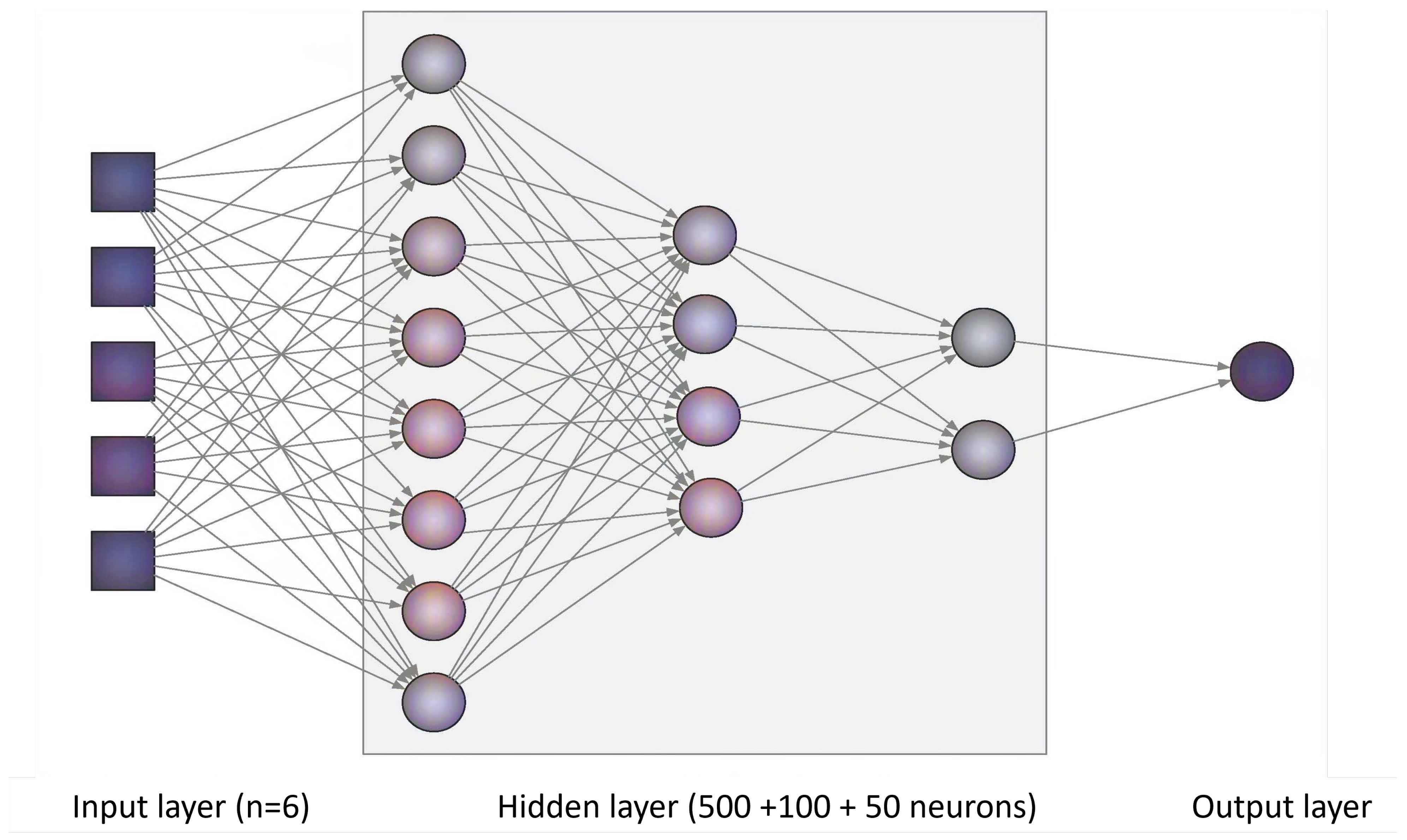
In this work, Sentinel-2 data were sought for Byers Peninsula. Several options were analyzed: the use of the Sentinel-2 Global Mosaic (S2GM) and the use of daily imagery. The use of mosaics was discarded, as they do not provide an acceptable result due to the high presence of clouds and snow in the region. Out of more than 200 daily images, in principle only one image could be used, the Sentinel-2-A image from 28 March 2016, at 13:29. The rest have many clouds and snow. The image was corrected for the atmosphere using Sen2Cor in SNAP to obtain the L2A-level product (BOA reflectivity). For this work, six radiometric indexes are applied to the BOA reflectivity (Table 1). In this Sentinel-2 image, of the 49 soil samples, 12 fall in areas of the image with clouds or snow, leaving 49 12 = 37 samples available. However, a WorldView-2 image of Byers Peninsula taken on 2 February 2011 at 13:31 is available for this study. The spatial resolution of the image is 0.5 m for the panchromatic band and 2 m for the others. It is a BOA reflectivity image corrected for the atmosphere using ATCOR-2 in ERDAS. We also used this image because it is free of clouds. The 49 soil samples fall in areas without clouds and snow in the WorldView-2 image. The same six radiometric indexes were computed (Table 1).

2.4. Modeling

Many authors have tried different techniques to model the spatial distribution of soil properties using explanatory variables. In [23], we can find an extensive review of the works on digital soil mapping published between 2003 and 2021. This review is based on 244 works on modeling soil properties on a broad scale (>10,000 km 2 ). In bare soils of the Antarctic maritime areas, mapping of soil texture by [29] could be a reference point for our approach. We opted to compare two methods, a deep learning neural network [27] (Figure 2) and linear regression, to find the best straight line that describes the relationship between the dependent variable and the independent variables. Although it is a straightforward algorithm, linear regression is a powerful tool due to its simplicity and interpretability.
To generate a nonlinear regression model, we defined and trained a multilayer perceptron [46] (Figure 2). This is a common resource to solve problems where a linear approach is not good enough [47,48]. In summary, the topology of the neural network used in this work is described as follows:
  • Input layer (size = 6);
  • First hidden layer (500 neurons);
  • Second hidden layer (100 neurons);
  • Third hidden layer (50 neurons);
  • Output layer (1 neuron).
The model was trained using the mean-squared error (MSE) loss function [49], while the optimizer chosen for this purpose was Adam [50].
Multiple linear regression (MLR) was used to establish relationships between soil properties and explanatory variables. The linear regression model assumes a linear relationship between the inputs and outputs, this relationship being represented by a linear equation (Equation (1)):
Y = β 0 + β 1 X 1 + β 2 X 2 + + β p X p + e ,
where Y is the dependent variable (soil property), β 0 is the order at the origin or bias, β 1 β p are the coefficients of the independent variables ( X 1 X p bands and radiometric indexes) that determine the slope of the line, and e is the stochastic residual or difference between the model’s predictions and the actual values, which is assumed to be normally distributed with zero mean and constant variance. The analysis determined the variables using a backward stepwise selection procedure and Akaike information criterion (AIC) to find the model that best explains the data with the fewest parameters. Backwards stepwise regression with the Akaike information criterion (AIC) is a variable selection method that starts with a model including all possible predictor variables and iteratively removes the least significant variable at each step. At each stage, the AIC is calculated, which measures the quality of the model by considering both the fit of the model and its complexity, penalizing models with more variables to prevent overfitting. The process continues until no further improvement in the AIC is possible by removing additional variables, resulting in a model that seeks to balance simplicity with predictive power.
The training process in linear regression involves adjusting the values of β 0 , β 1 , β 2 , β n to minimize the mean-squared error (MSE) between predictions and actual values. Once the model has been trained, it can be used to make predictions on new data.

2.5. Validation and Statistical Analysis

The prediction models were validated using leave-one-out cross-validation (LOOCV). The mean absolute error (MAE) and root-mean-squared error (RMSE) were used to evaluate the prediction accuracy of different prediction models. The model with the lowest RMSE and MAE values is determined to be the most accurate. Their equations are expressed as Equations (2) and (3).
M A E = i = 0 n | O i P i | 2 n
R M S E = i = 0 n ( O i P i ) 2 n ,
where O i and P i are the observed and predicted contents, respectively.

3. Results and Discussion

3.1. Analysis of Soil Properties

In Table 2, we present the results of the laboratory analysis carried out on the 49 soil samples. It is important to note that the soils are poor in organic carbon (average OC 1.14%) with a maximum of 11.92% measured in the sample (40, in the beach; see Figure 1). Other samples with values near the maximum are samples 38 and 42, taken on the vegetated soils of the beach. But, the soils of the Byers Plateau (plot A, Figure 1) are poor in organic carbon. However, even if the organic carbon is very low (minimum 0.31 %), there are always iron chelates (minimum of 53.60 mg/kg in sample 26, with 0.41 of OC %). In addition, when organic carbon is present in soils, about 15% is in the form of dissolved organic carbon. The maximum content of organic carbon is 11.92 g/100 g of soil in sample 40, and 3.671 g corresponds to DOC. This amount represents about 1/3 of the organic carbon in the sample. This seems to indicate a release of organic carbon and Fe into the Antarctic Spodic cryosol environment, which is described by [14]. All Spodic cryosols contain large amounts of carbon, nitrogen, and iron complexed with organic matter in the topsoil [51]. Mosses and lichens are the organisms that contribute the most C and N (primary source) to the soil organic matter on Byers Peninsula [52]. The relationship between organic carbon and iron complexes in the soils of Byers Peninsula, occupied by mosses and lichens, appears to be very close. The soil with vegetation had the highest concentrations of iron chelates (1768 ± 374.26 mg kg 1 ). Finally, this work modeled soil pH H2O, which was found to be near neutral in most cases (average pH: 7.3). However, there were significant differences in the surface samples colonized by plants. These samples were significantly more acidic (pH: 5.07 ± 0.1) than the rest of the soils, which had an average pH of 7.32 ± 0.72. The work in [14] found that the soils with ornithogenic origin on Clark Peninsula, near the Wilkes Station (66° 15 25 S 110° 31 37 E) in Antarctica, have higher pH values than the soils influenced by geological substrata. However, Ref. [40] found that ornithogenic soils of Byers Peninsula have a pH value close to 5, more acidic than the soils in the Byers Plateau. Ornithogenic soils were not studied in Byers. However, the soils occupied by mosses exhibit the lowest pH values (5.07 ± 0.72). The explanation for this discrepancy with the work of [53] could be related to the nature of the rocks in the substrate. In Byers, pyroclastic and marine sedimentary rocks show the presence of carbonates, so in the case of Byers, the substrates are generally neutral with pH values slightly greater than 7.0 [19,21,40].

3.2. Generated Models and Maps of Soil Properties

The deep learning model uses 6 explanatory variables (Figure 2), which are the spectral indexes found in Table 1; thus, the significance of each variable varied across individual pixels. Therefore, determining the most crucial variables in predicting each soil property using this approach is challenging. On the other hand, although linear regression models have limitations, especially when the relationships between variables are nonlinear, they are a powerful tool due to their simplicity, interpretability, and computational efficiency. Table 3 summarizes the results of the LRM analysis for pH, DOC, and organic Fe.
Of the six spectral indices calculated, only three are included as significant variables in the models. Fe3 and Oxides are explanatory variables in all three models of the soil properties, while IR700 (the inverse of red) is significant only in the model of dissolved organic carbon. The R2 adjustment of these models is moderately low, with an R2 of 0.53 for the pH model, 0.69 for the DOC model, and 0.63 for organic Fe. All variables in the three models passed the significance test (p-level column below 0.05). The beta coefficient value represents the weight of the variable in the model. The Oxides spectral index had the highest values in all three models.
Table 4 presents the linear regression models constructed using spectral indices from the WorldView-2 image. The R2 of fit is lower in the pH and organic Fe models, but higher in the DOC model (R2 0.49 for pH model, R2 0.89 for DOC model, and R2 0.41 for organic Fe) than in the models built with the spectral indices on the Sentinel-2 image. As with the linear models constructed using the indices calculated in the Sentinel image (Table 3), all explanatory variables passed the model significance test with p-levels below 0.05. However, the variables included in the models differ. Only the spectral index (Fe3) is present in the pH and organic Fe models, with different values, but the same sign (negative in all six models). The spectral index that measures brightness (MSBI) plays an important role in the DOC and organic Fe models performed with the WorldView-2 images.

3.3. Spatial Distribution of Soil Properties

Since 2011, machine learning has become the most popular way to predict properties in digital soil mapping (DSM). Refs. [54,55] have also seen this trend. For [23], there are some reasons for this increasing use of this type of soil mapping tools. Machine learning and deep learning [55] techniques are good at understanding complicated relationships between soil properties and many environmental factors. They usually work better than older statistical methods and mapping techniques. In addition, computers are now more powerful and have new technologies, which makes it easier and faster to create soil maps using large amounts of data. Machine learning is a nonparametric method that does not require any hypothesis about the distribution and stationarity, which are no longer valid with large spatial extents and legacy data. However, machine learning and deep learning predictive models focus on prediction performance and overlook the importance of pedological knowledge [23]. Linear regression models can be used to create digital soil maps using structural equations, and they are useful for both predictive mapping and enhancing pedological knowledge [56,57].
The pH, DOC, and organic Fe models with the highest accuracy in this study were: a deep learning model for pH built on a Sentinel image with an MAE of 0.51, an RMSE of 0.70, and an R2 with residuals of −0.49; a linear regression model for DOC built on a Sentinel image with an MAE of 189.39, an RMSE of 342.23, and an R2 with a residual of 0.0; and a deep learning model for organic Fe with an MAE of 116.20, an RMSE of 209.93, and an R2 of −0.05. Table 5 presents the error analysis results for each model. To be selected as the optimal model, it must meet the criteria of having the lowest MAE and RMSE, while also ensuring that the errors do not correlate with the measured values.
The linear regression models (Table 3 and Table 4) of soil properties were extended across the entire Byers Peninsula using the Sentinel-2 and WorldView-2 images. In Figure 3, Figure 4 and Figure 5, we can see the spatial distribution of the DOC (mg/L), organic Fe (mg/kg), and pH models built with deep learning (DL), linear regression on Sentinel-2 (LRM_S), and linear regression on the WorldView-2 image (LRM_VW). Also, the comparison between the estimated values is presented in linear graphs. The types of lines have been assigned taking into account the error metric of each model (Table 5). Black color represents the values of the properties in each soil; the red line represents the model with the lowest MAE and RMSE; the dotted gray line represents the models with the highest MAE and RMSE. The figures consist of images of the extended models with the name of the approach in the upper left corner (DL, LRM_S, or LRM_VW) and one graph displaying the values for each sample, measured and estimated with each model. The images have not been cropped by the line of the coast, but the area of the Sentinel-2 image for which the soil property models would be valid has been highlighted.

3.4. Dissolved Organic Carbon (DOC) Models

Dissolved organic carbon has a different distribution depending on the model. The DOC models obtained from Sentinel-2 images show higher values of DOC in coastal areas and on beaches. This distribution is consistent with areas that have a higher presence of fauna and vegetation. These results are similar to those obtained in many other studies conducted on Byers Peninsula [14,21,40,51,58,59]. Mossy soils also exhibit a comparable relationship of significant amounts of organic Fe complexes, indicating that plant activity accelerates the weathering of primary minerals [14,20]. The accompanying graphs for the extended DOC models (Figure 3) show that deep learning (red line) best fits the data, while linear regression with the Sentinel-2 image performs the worst. However, the linear model with Sentinel-2 (gray dotted line) appears to fit the highest DOC values very well. Table 5 displays the MAE and RMSE indices for these DOC models, along with the correlation between the residuals and soil values. Based on the errors metric, the DL model appears to be the most accurate. However, it is important to note that the residuals of this model are highly correlated with the soil values (R2 0.68). The issue with this model is that it does not account for the high DOC soil values. On the other hand, the WorldView model (yellow line) shows no correlation between the values and residual.

3.5. Organic Fe Models

In the case of Fe chelates, the highest values are also found on the beaches and along the coast, following the geological patterns described by [40]. These areas are characterized by basalts and pyroclastic rocks. The spatial distribution pattern is similar to that of DOC. The indexes calculated using Sentinel-2 images produce the best models, while the estimations using WorldView-2 images (gray dotted line) perform poorly (see Table 5).

3.6. pH Models

The spatial distribution of the pH values estimated with DL and LRM and calculated based on the Sentinel-2 image shows the influence of the geological substrate. The highest pH values, in black in the maps (Figure 5), are associated with the distribution of basaltic and volcanic rocks [60] and agree with the surface pH values of the profiles of these zones of [40]. The pH values below 5.0 are also consistent with the location of the ornithogenic soils described by this author in Byers. On the other hand, the model created using the WorldView-2 image displays a distribution of pH values around 5.0, which are present in all low-lying areas associated with the valley bottom deposits [21,31]. However, only the soil samples taken from plot A (38 to 45) show pH values below 6.0. According to the studies on the Byers soils consulted in this work, the soils in these depressed areas, covered with fine sediments and incipient vegetation, present the lowest pH values. Nevertheless, these results were not found in the soils of the Byers Plateau (plot A, Figure 1), as they show pH values over 6.5. However, the pH model created using the indexes of the WorldView-2 image provides spatial estimations that agree with the pH values measured in various studies of Byers’ soils, despite producing the worst linear fits (R2 0.49) (e.g., [16,19,39]). The graphs in the figure indicate that this model tends to underestimate pH values in the soils of the Byers Plateau (up to sample 37, as shown in Figure 1). However, it accurately adjusts to lower pH values associated with beach areas (samples between 37 and 49, as shown in Figure 1), where there is more vegetation development [21]. The model with the worst pH estimation is LMR-S_pH, with an MAE of 3.04 and an RMSE of 3.53. The residuals are highly correlated with the estimations, with an R2 of 0.99. This model overestimates low pH values and underestimates higher values, making it inaccurate in its distribution of values. However, it does present a better linear fit (R2 0.54) than the pH model built with the spectral index in the WorldView image (R2 0.49). On the other hand, LRM_WV_pH presents lower MAE and RMSE values and the lowest residual correlation (−0.43; see Table 5).
We utilized spectral indexes from Sentinel-2 and WorldView-2 images as soil predictors. Remote sensing data can provide detailed information on soil properties, as bare surface reflectance is an intrinsic property of the soil material and may indicate soil attributes such as mineralogy [28]. This assumption is more applicable in regions with limited vegetation, such as Antarctica; Ref. [29] utilized Sentinel-2 spectral indexes, like the Soil Adjusted Vegetation Index (SAVI) and Normalized Difference Vegetation Index (NDVI), as predictor variables to map soil texture models in the bare soils of maritime Antarctica. A Boolean (0–1) vegetation layer was obtained using these spectral indexes, and the CHELSA net primary productivity (NPP) was used to represent the influence of vegetation or fauna activity, mainly penguins. However, in Byers Peninsula, vegetation cover is very scarce or practically non-existent [7], so we considered other radiometric indices more suitable to carry out this analysis. The radiometric indices used in this analysis are closely related to the geochemical composition and color of the bare soils on Byers Peninsula (see Table 1).

3.7. Searching Areas of Biological Occupation

This section provides examples of the implementation of the study. Figure 6 displays a map of Byers Peninsula, highlighting areas with concentrations of DOC and organic iron within the range of values found in the studied vegetated soils (soils 38 to 45; see Figure 1) using geochemical criteria. To make this classification, the best DOC model (DL) and the best organic Fe (LRM_S_Fe) model have been used (Table 5). Areas that meet the geochemical requirements specified in the map legend may be preferred for designing wildlife or vegetation studies in Byers. The second example could be applied in the search for ornithogenic soils that have not yet been discovered or studied Figure 7. In this new classification, the models for pH, DOC, and organic Fe that have provided the lowest values of the MAE and RMSE were used (Table 5). The values of the variables have been established following the analyses of the ornithogenic soil profiles studied by [40] in Byers Peninsula.

4. Conclusions

This study focused on Byers Peninsula, a significant ice-free region in maritime Antarctica. The Spanish Polar Program has been actively involved in environmental research in this area since 2006. The study emphasizes the importance of using a noninvasive method to locate and monitor areas of Byers Peninsula that experience significant nutrient and organic matter transfer due to biological activity during the brief Antarctic summer. Various species of birds and marine mammals are primarily responsible for this activity. The research aims to determine the most effective method for digital mapping (DSM) using optical satellite images. Soil properties such as dissolved organic carbon, organic complexes of iron, and pH, which are linked to biological activity, will also be analyzed. This study aims to identify robust models to track areas with ornithogenic soils and regions in Byers Peninsula capable of supporting substantial biological development by comparing the performance of linear regression and deep learning models. The deep learning (DL) model provided the best fits of the modeled properties, showing the lowest MAE and RMSE. However, the models exhibited significant correlations between the values of the variables and the residuals. The analysis suggests that DL models perform well in predicting values near the mean of the modeled variables, with the prediction error increasing or decreasing as the variable value deviates from the mean. On the contrary, LRM models do not exhibit this issue. Furthermore, the study found that the use of spectral indices with Sentinel-2 images yielded significantly better results. Perhaps the best contribution of this study is that Sentinel-2 images, which have a high temporal resolution and are also free, provide better estimates using both the DL and RLM methods.

Author Contributions

Conceptualization, S.d.C.F. and R.R.-C.; methodology, S.d.C.F. and R.R.-C.; software, R.M.; validation, S.d.C.F. and J.R.; formal analysis, S.d.C.F., R.M. and J.P.; investigation, S.d.C.F., J.R. and J.P.; resources, J.R. and R.M.; data curation, S.d.C.F. and R.M.; writing—original draft preparation, S.d.C.F.; writing—review and editing, R.M.; visualization, S.d.C.F., R.M. and R.R.-C.; supervision, S.d.C.F. and R.M.; project administration, S.d.C.F. and J.F.C.; funding acquisition, S.d.C.F. and J.F.C. All authors have read and agreed to the published version of the manuscript.

Funding

This research and the APC were funded by Ministerio de Ciencia e Innovación: PID2021-127060OB-I00, PID2020-113051RB-C31, PID2020-115269GB-I00, and PTDC/CTE-GIX/119582/2010.

Data Availability Statement

Publicly available datasets were analyzed in this study, as stated in the paper.

Conflicts of Interest

The authors declare no conflicts of interest.

References

  1. Velázquez, D.; Lezcano, M.Á.; Frias, A.; Quesada, A. Ecological relationships and stoichiometry within a Maritime Antarctic watershed. Antarct. Sci. 2013, 25, 191–197. [Google Scholar] [CrossRef]
  2. Barbosa, A.; De Mas, E.; Benzal, J.; Diaz, J.I.; Motas, M.; Jerez, S.; Pertierra, L.; Benayas, J.; Justel, A.; Lauzurica, P.; et al. Pollution and physiological variability in gentoo penguins at two rookeries with different levels of human visitation. Antarct. Sci. 2013, 25, 329–338. [Google Scholar] [CrossRef]
  3. Quesada, A.; Camacho, A.; Rochera, C.; Velázquez, D. Byers Peninsula: A reference site for coastal, terrestrial and limnetic ecosystem studies in maritime Antarctica. Polar Sci. 2009, 3, 181–187. [Google Scholar] [CrossRef]
  4. de Pablo, M.A.; Ramos, M.; Molina, A. Thermal characterization of the active layer at the Limnopolar Lake CALM-S site on Byers Peninsula (Livingston Island), Antarctica. Solid Earth 2014, 5, 721–739. [Google Scholar] [CrossRef]
  5. Lyons, W.B.; Welch, K.; Welch, S.; Camacho, A.; Rochera, C.; Michaud, L.; Dewit, R.; Carey, A. Geochemistry of streams from byers peninsula, Livingston Island. Antarct. Sci. 2013, 25, 181–190. [Google Scholar] [CrossRef]
  6. Toro, M.; Granados, I.; Pla, S.; Giralt, S.; Antoniades, D.; Galán, L.; Cortizas, A.M.; Lim, H.S.; Appleby, P.G. Chronostratigraphy of the sedimentary record of limnopolar lake, Byers peninsula, Livingston island, Antarctica. Antarct. Sci. 2013, 25, 198–212. [Google Scholar] [CrossRef]
  7. Vera, M.L.; Fernández-Teruel, T.; Quesada, A. Distribution and reproductive capacity of Deschampsia antarctica and Colobanthus quitensis on Byers Peninsula, Livingston Island, South Shetland Islands, Antarctica. Antarct. Sci. 2013, 25, 292–302. [Google Scholar] [CrossRef]
  8. Villaescusa, J.A.; Casamayor, E.O.; Rochera, C.; Quesada, A.; Michaud, L.; Camacho, A. Heterogeneous vertical structure of the bacterioplankton community in a non-stratified Antarctic lake. Antarct. Sci. 2013, 25, 229–238. [Google Scholar] [CrossRef]
  9. Emslie, S.D.; Polito, M.J.; Patterson, W.P. Stable isotope analysis of ancient and modern gentoo penguin egg membrane and the krill surplus hypothesis in Antarctica. Antarct. Sci. 2013, 25, 213–218. [Google Scholar] [CrossRef]
  10. Nakai, R.; Shibuya, E.; Justel, A.; Rico, E.; Quesada, A.; Kobayashi, F.; Iwasaka, Y.; Shi, G.Y.; Amano, Y.; Iwatsuki, T.; et al. Phylogeographic analysis of filterable bacteria with special reference to Rhizobiales strains that occur in cryospheric habitats. Antarct. Sci. 2013, 25, 219–228. [Google Scholar] [CrossRef]
  11. Kopalová, K.; Van de Vijver, B. Structure and ecology of freshwater benthic diatom communities from Byers Peninsula, Livingston Island, South Shetland Islands. Antarct. Sci. 2013, 25, 239–253. [Google Scholar] [CrossRef]
  12. Benayas, J.; Pertierra, L.R.; Tejedo, P.; Lara, F.; Bermudez, O.; Hughes, K.A.; Quesada, A. A review of scientific research trends within ASPA No. 126 Byers Peninsula, South Shetland Islands, Antarctica. Antarct. Sci. 2013, 25, 128–145. [Google Scholar] [CrossRef]
  13. Campbell, I.; Claridge, G. Antarctica: Soils, Weathering Processes and Environment; Elsevier Science: Amsterdam, The Netherlands, 1987. [Google Scholar]
  14. Beyer, L. Properties, formation, and geo-ecological significance of organic soils in the coastal region of East Antarctica (Wilkes Land). CATENA 2000, 39, 79–93. [Google Scholar] [CrossRef]
  15. Ugolini, F.; Bockheim, J. Antarctic soils and soil formation in a changing environment: A review. Geoderma 2008, 144, 1–8. [Google Scholar] [CrossRef]
  16. Simas, F.N.B.; Schaefer, C.E.G.R.; Michel, R.F.; Francelino, M.R.; Bockheim, J.G. Soils of the South Orkney and South Shetland Islands, Antarctica. In The Soils of Antarctica; Springer International Publishing: Cham, Switzerland, 2015; pp. 227–273. [Google Scholar] [CrossRef]
  17. Ugolini, F. Ornithogenic soils of Antarctica. Antarct. Terr. Biol. 1972, 20, 181–193. [Google Scholar]
  18. Tatur, A.; Myrcha, A. Ornithogenic Ecosystems in the Maritime Antarctic-Formation, Development and Disintegration. In Ornithogenic Ecosystems in the Maritime Antarctic—Formation, Development and Disintegration; Ecological Studies; Springer: Berlin/Heidelberg, Germany, 2002; pp. 161–186. [Google Scholar]
  19. Navas, A.; López-Martínez, J.; Casas, J.; Machín, J.; Durán, J.J.; Serrano, E.; Cuchi, J.A. Soil characteristics along a transect on raised marine surfaces on Byers Peninsula, Livingston Island, South Shetland Islands. In Antarctica: Contributions to Global Earth Sciences; Springer: Berlin/Heidelberg, Germany, 2006; pp. 467–473. [Google Scholar]
  20. Bölter, M.; Kandeler, E. Microorganisms and microbial processes in Antarctic soils. In Cryosols: Permafrost-Affected Soils; Springer: Berlin/Heidelberg, Germany, 2004; pp. 557–572. [Google Scholar]
  21. Otero, X.; Fernández, S.; de Pablo Hernandez, M.; Nizoli, E.; Quesada, A. Plant communities as a key factor in biogeochemical processes involving micronutrients (Fe, Mn, Co, and Cu) in Antarctic soils (Byers Peninsula, maritime Antarctica). Geoderma 2013, 195, 145–154. [Google Scholar] [CrossRef]
  22. Gamble, A.; Howe, J.; Delaney, D.; Van Santen, E.; Yates, R. Iron chelates alleviate iron chlorosis in soybean on high pH soils. Agron. J. 2014, 106, 1251–1257. [Google Scholar] [CrossRef]
  23. Chen, S.; Arrouays, D.; Leatitia Mulder, V.; Poggio, L.; Minasny, B.; Roudier, P.; Libohova, Z.; Lagacherie, P.; Shi, Z.; Hannam, J.; et al. Digital mapping of GlobalSoilMap soil properties at a broad scale: A review. Geoderma 2022, 409, 115567. [Google Scholar] [CrossRef]
  24. Turner, D.; Lucieer, A.; Malenovský, Z.; King, D.; Robinson, S.A. Assessment of Antarctic moss health from multi-sensor UAS imagery with Random Forest Modelling. Int. J. Appl. Earth Obs. Geoinf. 2018, 68, 168–179. [Google Scholar] [CrossRef]
  25. Román, A.; Tovar-Sánchez, A.; Fernández-Marín, B.; Navarro, G.; Barbero, L. Characterization of an antarctic penguin colony ecosystem using high-resolution UAV hyperspectral imagery. Int. J. Appl. Earth Obs. Geoinf. 2023, 125, 103565. [Google Scholar] [CrossRef]
  26. Zmarz, A.; Rodzewicz, M.; Dąbski, M.; Karsznia, I.; Korczak-Abshire, M.; Chwedorzewska, K.J. Application of UAV BVLOS remote sensing data for multi-faceted analysis of Antarctic ecosystem. Remote Sens. Environ. 2018, 217, 375–388. [Google Scholar] [CrossRef]
  27. Fernández, S.; Muñiz, R.; Peón, J.; Rodríguez-Cielos, R.; Pisabarro, A.; Calleja, J. Machine learning and linear regression models for mapping soil properties and albedo in periglacial areas using Sentinel imagery (Byers Peninsula, Marine Antarctica). Sensors 2024, in press. [Google Scholar]
  28. Minasny, B.; McBratney, A. Digital soil mapping: A brief history and some lessons. Geoderma 2016, 264, 301–311. [Google Scholar] [CrossRef]
  29. Siqueira, R.G.; Moquedace, C.M.; Francelino, M.R.; Schaefer, C.E.; Fernandes-Filho, E.I. Machine learning applied for Antarctic soil mapping: Spatial prediction of soil texture for Maritime Antarctica and Northern Antarctic Peninsula. Geoderma 2023, 432, 116405. [Google Scholar] [CrossRef]
  30. Quayle, W.C.; Convey, P.; Peck, L.S.; Ellis-Evans, C.J.; Butler, H.G.; Peat, H.J. Ecological responses of maritime Antarctic lakes to regional climate change. Antarct. Res. Ser. 2003, 79, 159–170. [Google Scholar]
  31. Lopez-Martinez, J.; Thomson, M.; Arche, A.; Bjorck, S.; Ellis-Evans, J.C.; Hatway, B.; Hernández-Cifuentes, F.; Hjort, C.; Ingolfsson, O.; Ising, J.; et al. Geomorphological Map of Byers Peninsula, Livingston Island; British Antarctic Survey: Cambridge, UK, 1996. [Google Scholar]
  32. Björck, S.; Hjort, C.; Ingólfsson, O.; Zale, R.; Ising, J. Holocene deglaciation chronology from lake sediments. In Geomorphological map of Byers Peninsula, Livingston Island; BAS GEOMAP Series, Sheet; BAS: Cambridge, UK, 1996; pp. 49–51. [Google Scholar]
  33. Hobbs, G. The Geology of the South Shetland Islands: IV. The Geology of Livingston Island; British Antarctic Survey: Cambridge, UK, 1968. [Google Scholar]
  34. Hathway, B. Nonmarine sedimentation in an Early Cretaceous extensional continental-margin arc, Byers Peninsula, Livingston Island, South Shetland Islands. J. Sediment. Res. 1997, 67, 686–697. [Google Scholar] [CrossRef]
  35. van Zinderen Bakker, E.M. Palaeoecology of Africa & of the Surrounding Islands & Antarctica; AA Balkema: Rotterdam, The Netherlands, 1966; Volume 16. [Google Scholar]
  36. Simms, A.R.; Milliken, K.T.; Anderson, J.B.; Wellner, J.S. The marine record of deglaciation of the South Shetland Islands, Antarctica since the Last Glacial Maximum. Quat. Sci. Rev. 2011, 30, 1583–1601. [Google Scholar] [CrossRef]
  37. Bañón, M.; Justel, A.; Velázquez, D.; Quesada, A. Regional weather survey on Byers Peninsula, Livingston Island, South Shetland Islands, Antarctica. Antarct. Sci. 2013, 25, 146–156. [Google Scholar] [CrossRef]
  38. Hall, M.; Allinson, D. Assessing the effects of soil grading on the moisture content-dependent thermal conductivity of stabilised rammed earth materials. Appl. Therm. Eng. 2009, 29, 740–747. [Google Scholar] [CrossRef]
  39. Navas, A.; López-Martínez, J.; Casas, J.; Machín, J.; Durán, J.J.; Serrano, E.; Cuchi, J.A.; Mink, S. Soil characteristics on varying lithological substrates in the South Shetland Islands, maritime Antarctica. Geoderma 2008, 144, 123–139. [Google Scholar] [CrossRef]
  40. Moura, P.A.; Francelino, M.R.; Schaefer, C.E.G.; Simas, F.N.; de Mendonça, B.A. Distribution and characterization of soils and landform relationships in Byers Peninsula, Livingston Island, Maritime Antarctica. Geomorphology 2012, 155–156, 45–54. [Google Scholar] [CrossRef]
  41. Mars, J.C.; Rowan, L.C. ASTER spectral analysis and lithologic mapping of the Khanneshin carbonatite volcano, Afghanistan. Geosphere 2011, 7, 276–289. [Google Scholar] [CrossRef]
  42. Escadafal, R.; Girard, M.C.; Courault, D. Munsell soil color and soil reflectance in the visible spectral bands of landsat MSS and TM data. Remote Sens. Environ. 1989, 27, 37–46. [Google Scholar] [CrossRef]
  43. Gitelson, A.A.; Kaufman, Y.J.; Merzlyak, M.N. Use of a green channel in remote sensing of global vegetation from EOS-MODIS. Remote Sens. Environ. 1996, 58, 289–298. [Google Scholar] [CrossRef]
  44. Misra, A.; Prasad, R.C.; Chauhan, V.S.; Srilakshmi, B. A theoretical model for the electromagnetic radiation emission during plastic deformation and crack propagation in metallic materials. Int. J. Fract. 2007, 145, 99–121. [Google Scholar] [CrossRef]
  45. Hewson, R.; Robson, D.; Mauger, A.; Cudahy, T.; Thomas, M.; Jones, S. Using the Geoscience Australia-CSIRO ASTER maps and airborne geophysics to explore Australian geoscience. J. Spat. Sci. 2015, 60, 207–231. [Google Scholar] [CrossRef]
  46. Murtagh, F. Multilayer perceptrons for classification and regression. Neurocomputing 1991, 2, 183–197. [Google Scholar] [CrossRef]
  47. Muñiz, R.; Cuevas-Valdés, M.; de la Roza-Delgado, B. Milk quality control requirement evaluation using a handheld near infrared reflectance spectrophotometer and a bespoke mobile application. J. Food Compos. Anal. 2020, 86, 103388. [Google Scholar] [CrossRef]
  48. Gaudart, J.; Giusiano, B.; Huiart, L. Comparison of the performance of multi-layer perceptron and linear regression for epidemiological data. Comput. Stat. Data Anal. 2004, 44, 547–570. [Google Scholar] [CrossRef]
  49. Hodson, T.O.; Over, T.M.; Foks, S.S. Mean squared error, deconstructed. J. Adv. Model. Earth Syst. 2021, 13, e2021MS002681. [Google Scholar] [CrossRef]
  50. Kingma, D.P.; Ba, J. Adam: A method for stochastic optimization. arXiv 2014, arXiv:1412.6980. [Google Scholar]
  51. Beyer, L.; Bölter, M. Chemical and biological properties, formation, occurrence and classification of Spodic Cryosols in a terrestrial ecosystem of East Antarctica (Wilkes Land). CATENA 2000, 39, 95–119. [Google Scholar] [CrossRef]
  52. da Silva, J.P.; Lelis Leal de Souza, J.J.; Mercês Barros Soares, E.; Schaefer, C.E.G. Soil organic matter accumulation before, during, and after the last glacial maximum in Byers Peninsula, Maritime Antarctica. Geoderma 2022, 428, 116221. [Google Scholar] [CrossRef]
  53. Blume, H.P.; Kuhn, D.; Bölter, M. Soils and soilscapes. In Geoecology of Antarctic Ice-Free Coastal Landscapes; Springer: Berlin/Heidelberg, Germany, 2002; pp. 91–113. [Google Scholar]
  54. Arrouays, D.; Poggio, L.; Salazar Guerrero, O.A.; Mulder, V.L. Digital soil mapping and GlobalSoilMap. Main advances and ways forward. Geoderma Reg. 2020, 21, e00265. [Google Scholar] [CrossRef]
  55. Padarian, J.; Minasny, B.; McBratney, A. Using deep learning to predict soil properties from regional spectral data. Geoderma Reg. 2019, 16, e00198. [Google Scholar] [CrossRef]
  56. Wadoux, A.M.C.; Minasny, B.; McBratney, A.B. Machine learning for digital soil mapping: Applications, challenges and suggested solutions. Earth-Sci. Rev. 2020, 210, 103359. [Google Scholar] [CrossRef]
  57. Ma, Y.; Minasny, B.; McBratney, A.; Poggio, L.; Fajardo, M. Predicting soil properties in 3D: Should depth be a covariate? Geoderma 2021, 383, 114794. [Google Scholar] [CrossRef]
  58. Abakumov, E.; Gagarina, E.; Sapega, V.; Vlasov, D.Y. Micromorphological features of the fine earth and skeletal fractions of soils of West Antarctica in the areas of Russian Antarctic stations. Eurasian Soil Sci. 2013, 46, 1219–1229. [Google Scholar] [CrossRef]
  59. Silvero, N.E.; Demattê, J.A.; de Souza Vieira, J.; de Oliveira Mello, F.A.; Amorim, M.T.A.; Poppiel, R.R.; de Sousa Mendes, W.; Bonfatti, B.R. Soil property maps with satellite images at multiple scales and its impact on management and classification. Geoderma 2021, 397, 115089. [Google Scholar] [CrossRef]
  60. Hathway, B.; Lomas, S. The jurassic–lower cretaceous Byers group, South Shetland islands, Antarctica: Revised stratigraphy and regional correlations. Cretac. Res. 1998, 19, 43–67. [Google Scholar] [CrossRef]
Figure 1. The location of Byers Peninsula (latitude 62° 34 35 S, longitude 61° 13 07 W) in the South Shetland Islands. The WorldView-2 image (projection EPSG:32720 WGS 84/UTM zone 20S) used in this study with the location of soil samples in plots A and B. Photo (A) corresponds to typical soil from plot A from the Byers Plateau. Photo (B) corresponds to organic soil from beaches (plot B).
Remotesensing 16 01192 g001
Figure 2. Simplified representation of the neural network topology used.
Remotesensing 16 01192 g002
Figure 3. Dissolved organic carbon (DOC mg/L). Models DL_DOC, LRM_S_DOC, and LRM_WV_DOC extended to the entire Byers Peninsula: DL and LRM_S were regionalized in Sentinel-2 imagery. LRM_WW used a WorldView-2 image. The values of DOC measured in the samples (line black), estimated with deep learning (DL) (line red), linear regression in the Sentinel image (LRM_S) and linear regression in WV (gray dotted line) are compared in the graph.
Remotesensing 16 01192 g003
Figure 4. Fe associated with organic matter (mg/kg). Organic Fe (Fe mg/kg). Models DL_Fe LRM_S_Fe, and LR_WV_Fe extended to the entire Byers Peninsula: DL and LRM_S were regionalized in the Sentinel-2 imagery. LRM_WW used the WorldView-2 image. The values of organic Fe measured in the samples (black line), estimated with deep learning (DL) (red line), linear regression in the Sentinel image (LRM_S), and linear regression in WV (gray dotted line) are compared in the graph.
Remotesensing 16 01192 g004
Figure 5. pH models. Models DL_pH; LRM_S_pH and LRM_WV_pH extended to the entire Byers Peninsula: DL and LRM_S were regionalized in the Sentinel-2 imagery. LRM-WW used the WorldView-2 image. The values of the pH measured in the samples (line black), estimated with deep learning (DL) (red line) and, in this case, linear regression in WV (LRM_WV), are in the yellow line because they show better predictions than LRM_S (gray dotted line).
Remotesensing 16 01192 g005
Figure 6. In red, areas with concentrations of DOC and organic iron within the range of values found in the vegetated soils studied.
Remotesensing 16 01192 g006
Figure 7. In red, areas prone to have ornithogenic soils, based on [40].
Remotesensing 16 01192 g007
Table 1. Radiometric indexes used in this study; the expression and Sentinel-2 bands involved in their formulation.
IndexesExpressionSentinel-2 BandsWV-2 BandsAuthors
Ferric iron (Fe3) ρ R E D ρ G R E E N B4-VIS- ρ RED
B3-VIS- ρ GREEN
B2-GREEN- ρ GREEN
B3-RED- ρ RED
[41]
Hue arctan 2 R G B 30.5 × ( G B ) B2-VIS- ρ BLUE
B3-VIS- ρ GREEN
B4-VIS- ρ BLUE
B1-BLUE- ρ BLUE
B2-GREEN- ρ GREEN
B3-RED- ρ RED
[42]
IR550 I R _ G R E E N = 1 ρ G R E E N B3-VIS- ρ GREENB2-GREEN- ρ GREEN[43]
IR700 I R _ R E D = 1 ρ R E D B5- ρ NIRB3-RED- ρ RED[43]
Missa Soil
Brightness Index
(MSBI) v2
M S B I =
0.406 × ρ G R E E N +
0.600 × ρ R E D +
0.645 × ρ N I R 1 +
0.243 × ρ N I R 2

B3-VIS- ρ GREEN
B4-VIS- ρ RED
B6-NIR- ρ NIR1
B8a-NIR- ρ NIR2

B0-PAN- ρ NIR1
B2-GREEN- ρ GREEN
B3-RED- ρ RED
B4-NIR1- ρ NIR2
[44]
I/O (Oxides)IO= ρ R E D ρ B L U E B2-VIS- ρ BLUE
B4-VIS- ρ RED
B1-BLUE- ρ BLUE
B3-RED- ρ RED
[45]
Table 2. Soil properties measured in the soil samples.
n 49MeanMinimumMaximumStd. Dev.
DOC (mg/kg)193.310.003671.09656.77
Organic Fe (mg/kg)286.0153.601768.00374.26
pH H 2 O7.325.078.260.72
Density (g/cm3)1.160.171.500.27
OC (%)1.140.3111.922.49
CLAY15.234.1332.425.33
SILT20.344.3738.598.39
SAND64.4543.8587.3811.26
Mn (g/Kg)6.401.7610.912.04
Ca (mg/kg)17.172.2029.207.62
Table 3. Summary of the linear regression models using Sentinel-2 spectral indices. The values of the standardized coefficients (Beta), the coefficients (B) of the line of best fit, and the significance of the models (p-level) are presented.
BetaStd. Err. of BetaBStd. Err. of Bp-Level
Intercept 6.4050.67470.00000
S_Fe30.44160.10692.9550.71490.00015
S_Oxides−0.79700.1069−1.5780.21160.00000
Variable: H 2 O pH; R = 0.74499237; R 2 = 0.55501364; Adjusted R 2 = 0.53566640; F (2.46) = 28.687 p
Intercept 2897.36523.54660.00000
S_Fe3−0.79040.09604796.81582.41670.00000
S_IR700−0.39920.1227−90.8227.91040.00216
S_Oxides1.12070.13332013.34239.40860.00000
Variable: DOC (mg/L); R = 0.84590926; R 2 = 0.71556248; Adjusted R 2 = 0.69659998; F (3.45) = 37.736 p
Intercept 782.16312.72500.01600
S_Fe3−0.47290.0956−1638.15331.34580.00001
S_Oxides0.85870.0956880.598.07850.00000
Variable: Organic Fe (mg/kg); R = 0.80217191; R 2 = 0.64347977; Adjusted R 2 = 0.62797889 F (2.46) = 41.512 p
Table 4. Summary of the linear regression models using WorldView-2 spectral indices. The values of the standardized coefficients (Beta), the coefficients (B) of the line of best fit, and the significance of the models (p-level) are presented.
BetaStd. Err. of BetaBStd. Err. of Bp-Level
Intercept 2.51461.39100.0775
WV_Fe31.17170.27755.84711.38490.0001
WV_IR7002.50890.82280.36870.12090.0039
WV_IR500−2.08430.7100−0.41430.14110.0053
WV_MSBI−0.62000.1391−7.38551.65680.0001
Variable: H 2 O pH; R = 0.73199980; R 2 = 0.53582371; Adjusted R 2 = 0.49362587; F (2.46) = 12.698 p
Intercept −728.0163.550.0001
WV_HUE−0.53510.05473−57,338.55864.860.0000
WV_Oxides0.12190.05341160.470.260.0273
WV_MSBI0.95590.0546810329.5590.850.0000
Variable: DOC (mg/L); R = 0.93861507; R 2 = 0.88099825; Adjusted R 2 = 0.87306480; F (3.45) = 111.05 p
WV_Fe3−0.86070.2981−2223.94770.2840.0060
WV_IR700−2.04990.8839−155.9867.2570.0251
WV_IR5001.81320.7627186.6078.4870.0218
WV_MSBI0.70010.14944318.06921.5690.0000
Variable: Organic Fe (mg/kg); R = 0.68146494; R 2 = 0.46439447; Adjusted R 2 = 0.415703 F (4.44) = 9.5375
Table 5. Error analysis. Deep learning (DL); linear regression model (LRM); WorlsView-2 image (WV2); dissolved organic carbon (DOC); iron associated with organic matter (Fe); R2 residuals are the correlation coefficient between estimations and residuals.
ImageModelMAERMSE R 2 Residuals
SentinelDL_pH0.510.70−0.49
SentinelLRM_pH3.043.53−0.99
WV2LRM_pH1.211.37−0.43
SentinelDL_DOC131.87156.200.68
SentinelLRM_DOC189.39343.230.00
WV2LRM_DOC202.52402.120.43
SentinelDL_Fe116.70209.93−0.05
SentinelLRM_Fe131.27219.350.00
WV2LRM_Fe2689.002756.65−0.80
Disclaimer/Publisher’s Note: The statements, opinions and data contained in all publications are solely those of the individual author(s) and contributor(s) and not of MDPI and/or the editor(s). MDPI and/or the editor(s) disclaim responsibility for any injury to people or property resulting from any ideas, methods, instructions or products referred to in the content.

