Abstract
Hyperspectral remote sensing technology is an advanced and powerful tool that enables fine identification of the numerous soil reflectance spectrum characteristics. Heavy metal(loid)s (HMs) are the primary pollutants affecting the soil biodiversity and ecosystem services. Estimating HMs’ concentrations in soils using hyperspectral data is an effective method but is challenging due to the effects of varied soil properties and measurement-related errors inflicted by atmospheric effects. This study focused on typical mining areas in the Fenwei Plain (FWP), China. Soil-related data were collected by leveraging airborne- and ground-based integrated remote sensing observations. The concentrations of eight HMs, namely copper (Cu), lead (Pb), zinc (Zn), nickel (Ni), chromium (Cr), cadmium (Cd), arsenic (As), and mercury (Hg), were measured by laboratory analysis from 100 in situ soil samples. Soil reflectance spectra were processed based on resampling and envelope methods. The combination datasets of the concentrations and optimal soil reflectance spectra were used to build the soil-related parameter retrieval models using three machine learning (ML) methods, and the feasibility of applying the high-performance retrieval model to estimate the HM concentrations in mining areas was evaluated and explored. Spectral analysis results show that four hundred and twenty-eight bands of five wavelength ranges are of high quality and obviously demonstrate the spectral characteristics selected to build the soil-related parameter models. The evaluation results of eight combination data subsets and three methods show that the preprocessing of spectral data (ground- and airborne-based reflectance) and soil samples with the random forest (RF) method can obtain higher accuracy than support vector machine (SVM) and partial least squares (PLS) methods, denoted as the AER-ACS-RF and GER-GCS-RF models (the average RMSE values of eight HMs were 2.61 and 2.53 mg/kg, respectively). The highest R2 values were observed in Cd and As, with an equal value of 0.98, followed by that of Pb (R2 = 0.97). The relative prediction deviation (RPD) values of Cu and AS were greater than 1.9. Moreover, the airborne-based AER-ACS-RF model presents a good mapping effect about the concentrations (mg/kg) of eight HMs in mining areas, ranging from 21.65 to 31.25 (Cu), 16.38 to 30.45 (Pb), 62.02 to 109.48 (Zn), 23.33 to 32.47 (Ni), 49.81 to 66.56 (Cr), 0.09 to 0.23 (Cd), 7.31 to 12.24 (As), and 0.03 to 0.17 (Hg), respectively.
1. Introduction
Soil-related heavy metal(loid)s (HMs) are one of the main pollutants leading to threats to soil biodiversity and numerous ecosystem services [1,2]. For example, Cu, Pb, Zn, Ni, Cr, Cd, As, and Hg are common pollutants in the soil environment [3,4], and their toxicity has potential hazards to human and animal health [5]. Driven by the growing demand for minerals, mining activities have expanded into biodiversity-rich ecosystems, which can cause a wide range of adverse impacts on soil pollution [6]. Therefore, estimating the HM parameters of soil is crucial for monitoring the soil’s environmental quality risks, especially in mining areas.
Hyperspectral remote sensing data with high-spectral, spatial, and temporal resolutions [7] provide unprecedented opportunities for mining exploration and environmental hazard monitoring [8,9,10]. Previous studies [11,12,13,14] have shown that it is feasible to quantitatively estimate the concentrations of soil-related HMs from the airborne-based hyperspectral imagery captured by onboard sensors, such as the Hyperspectral MAPper (HyMAP) sensor [15] and airborne visible/infrared imaging spectrometer (AVIRIS) [16]. Owing to high-dimension mixed spectra in hyperspectral data and the subtle spectral responses of HM concentrations, the most current methods [17,18,19] developed for estimating soil-related parameters are based on spectral pretreatment, spectral enhancement, and feature selection methods to optimize the raw reflectance, such as the first derivative (FD), logarithm of reciprocal (LR), and continuum removal (CR) methods. Based on these spectral analysis methods, the optimal relationships with soil spectral variables and HMs were identified and then used to build retrieval models for estimating the soil-related HM concentrations in real applications. For modeling methods, previous studies [11,19,20,21] have proven that ML-based regression algorithms (such as RF, SVM, and PLS) can be successfully applied to understand and model rich soil-related parameters.
In spite of the demonstrated feasibility of estimating HM concentrations, there are still many challenging problems in the quantitative estimation of soil-related HM concentrations and the accurate mapping of spatial distributions using airborne-based hyperspectral imagery, especially in practical applications [17]. The main factors are that the spatial heterogeneity of large field-of-view (FOV) aerial imaging is significant; the modeling process is affected by imbalanced samples measured in the area where soil-related HM concentrations severely exceed the standard [11]. The sensors [22] and atmospheric absorption [17] may produce measurement-related errors. Moreover, the field spectral reflectance measured in situ and soil samples form the basis of ground-based hyperspectral information and concentrations of soil-related HMs. The ground-based soil reflectance spectra of soil samples were commonly measured and recorded in situ or in the laboratory using spectroradiometers or spectrophotometers, which were successfully applied to estimate the contents of soil-related parameters [10,13,14,23,24,25].
Simultaneous and integrated airborne–ground hyperspectral data have rarely been used to quantify soil-related HM concentrations due to difficulties with synchronized data availability. Simultaneous and integrated airborne–ground remote sensing experiments need a large amount of human, material, and instrument resources at the same time. Simultaneous ground-based field measurements are crucial complementary components to airborne-based hyperspectral imagery for radiometric calibration and ground truth validation as they reduce the error mechanisms introduced by sensor noise and atmospheric effects. Therefore, incorporating airborne-based hyperspectral imagery and ground-based in situ data into the analysis can help address the challenges associated with the high-accuracy mapping of soil-related HM concentrations.
In summary, given that the ground- and airborne-based soil reflectance characteristics vary across wavelengths and in situ soil samples, there is a need to estimate high-accuracy concentrations of eight HMs from comprehensive observations simultaneously. The main purpose of this study is to develop a generalizable soil-related parameter estimation framework that achieves simultaneous and high-accuracy estimations of eight HM concentrations from both ground- and airborne-based hyperspectral data. The main contributions of this study can be concluded as follows:
- During the airborne-based hyperspectral imaging, in situ soil sampling, ground-based reflectance measurements, and radiometric calibration processes were conducted in typical mining areas in the FWP region.
- Soil hyperspectral reflectance libraries and HM concentrations were created based on airborne–ground simultaneous and integrated observations of 100 in situ soil samples, which fill the data gap in simultaneous airborne–ground measurements of eight soil-related parameters.
- Four hundred and twenty-eight bands of five optimal wavelength ranges with high-quality and obvious spectral characteristics were selected, and eight training data subsets were generated after the data preprocessing steps, including spectral resampling, envelope, and soil sample pruning processes.
- Soil-related parameter retrieval models based on three ML methods were built to boost the optimization of the retrieval model by quantifying the RMSE of each training and testing data subset.
- The concentrations of eight HMs obtained using the proposed retrieval model were estimated and mapped in mining areas for real applications.
The rest of this paper is organized as follows: Section 2 illustrates the details of the field measurements and their preprocessing steps among airborne-based hyperspectral remote sensing observations and simultaneous measurements of ground-based in situ data. This section introduces three ML methods with their corresponding parameters and modeling processes. Section 3 presents the evaluation results of eight combination data subsets within three regression methods and defines the best model for mapping the concentrations of eight HMs. Section 4 analyzes and discusses the sensitivity and application performance of the best model. Finally, conclusions and potential future research in soil-related parameter modeling for monitoring applications in eight HMs are drawn in Section 5.
2. Materials and Methods
2.1. Study Area
The FWP region (as shown in Figure 1a), located in the middle of three geological blocks (the Ordos, North China, and South China blocks), consists of the Fenhe and Weihe plains (also called the Guanzhong Plain) along with their surrounding terraces in the Yellow River Basin [26,27]. The FWP is the largest alluvial plain in the middle reaches of the Yellow River Basin, including the 11 cities of Xi’an, Xianyang, Weinan, Baoji, and Tongchuan in Shaanxi Province; Yuncheng, Linfen, Lvliang, and Jinzhong in Shanxi Province; and Luoyang and Sanmenxia in Henan Province. However, in 2018, the FWP, replacing the Pearl River Delta (PRD) region, was designated as one of the three key regions for the “Blue Sky Protection Campaign”, along with the Beijing–Tianjin–Hebei (BTH) and Yangtze River Delta (YRD) regions [28,29].
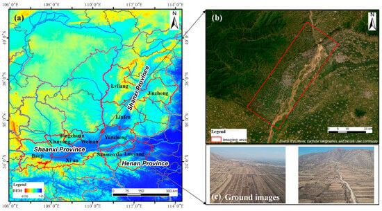
Figure 1.
Study area in the Fenwei Plain, China. (a) Geographical location of the FWP within the provinces and other administrative boundaries of China; (b) the relative position of Hancheng (imaging area) in the Fenwei Plain; (c) ground image examples.
Hancheng is located in the northeast of Weinan city in the FWP region and on the southeastern margin of the Ordos Basin (as shown in Figure 1b). Hancheng is characterized by its significant role in coal mining and coalbed methane development in China and is a typical medium- to high-ranked coal mining area with complex structural conditions [30]. Figure 1c presents some ground images in the area. However, beyond the economic benefits of coal mining, Hancheng has also faced environmental challenges, especially soil environmental quality, such as soil pollution, erosion, and acidification. Therefore, it requires comprehensive research that accurately estimates soil-related parameters and maps predicted distributions to safeguard soil health and ecosystem services in the face of ongoing coal mining development. This study presents a case study of mapping HM concentrations in the Hancheng mining area, using the measurement of the reflectance spectra (ground-based and airborne-based) and in situ soil samples to predict and estimate the concentrations of each HM element.
2.2. Field Measurements
2.2.1. Airborne- and Ground-Based Instruments
The airborne multi-modular imaging spectrometer (AMMIS) developed by the Shanghai Institute of Technical Physics (SITP) of the Chinese Academy of Sciences (CAS) [22] is positioned on the airborne imaging systems to capture electromagnetic radiation across different wavelengths or spectral bands in field photogrammetry experiments.
Table 1 illustrates the detailed parameters of the sensor. The AMMIS is designed with 256 bands in the visible, near-infrared (VNIR) spectral channel range spanning 0.4–0.95 μm, 512 bands in the short-wave infrared (SWIR) spectral channel range spanning 0.95–2.5 μm, and 128 bands in the thermal infrared (TIR) spectral channel range spanning 8–12.5 μm. At an observation altitude of 2 km, the different spatial resolutions of the VNIR and TIR spectral channels range from 0.5 m to 2 m. The spectral resolutions of the VNIR, SWIR, and TIR channels are 2.4 nm, 3 nm, and 32 nm, respectively. The large FOV of the three sensors (VNIR, SWIR, and TIR) is 40°, and the instantaneous fields of view (IFOVs) are 0.25, 0.5, and 1 mrad, respectively. The signal-to-noise ratio (SNR) test results of the three sensors are greater than 100 [22]. This hyperspectral imaging system captures data across multiple bands by push broom scanning, enabling the identification and differentiation of soil-related parameters based on their spectral characteristics. There are typical application fields with these multiple bands. For example, the VNIR and SWIR bands are used for vegetation identification and mineral detection, and land surface temperature (LST) and emissivity parameters are commonly retrieved from TIR bands for monitoring the thermal environment and thermal pollution detection applications.

Table 1.
Detailed instrument parameters of the airborne-based sensor.
In addition, ground-based instruments, including the Analytical Spectral Devices (ASD FieldSpec 3) spectroradiometer and the CIMEL CE318 photometer, were used for the synchronous measurements during the airborne-based hyperspectral imaging. The ASD FieldSpec 3 is a field-portable spectroradiometer manufactured by ASD Inc. (Boulder, CO, USA) with the model number of FS3 350-2500. The ASD provides continuous hyperspectral data ranging from 350 nm to 2500 nm (at 1 nm intervals and with 25 nm spectral resolution). The ground-based field spectra form the basis of distinguishing the various spectra of the HMs and extracting rich soil spectral information. The CE318 instrument is an automatic sun-and-sky photometer developed by CIMEL Electronique, measuring direct solar irradiance and sky radiance in the spectral range from 340 nm to 1640 nm. The four bands centered at 440 nm, 675 nm, 870 nm, and 1020 nm are commonly used to retrieve optical depth, and the NIR channel centered at 940 nm is used to estimate the atmospheric column water vapor (CWV).
2.2.2. Airborne- and Ground-Based Measurements
The aerial photogrammetry system with the AMMIS was used on 26 December 2021 to capture hyperspectral images in the Hancheng mining areas. Since the glass and filter were fixed in front of the sensor lens, the indoor radiometric calibration of the airborne-based sensor failed to be used. Therefore, in order to achieve high-precision calibration applications, ground-based radiometric calibration is needed. This study used a calibration approach based on grayscale artificial targets in the ground-based calibration field. As shown in Figure 2a, four grayscale artificial targets (5%, 20%, 40%, and 60%) provided by the Aerospace Information Research Institute (AIR) under the CAS were set on the square located on the flight area.
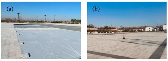
Figure 2.
Ground-based field measurements. (a) Radiometric calibration (optical) under ground-based grayscale artificial targets; (b) synchronous measurement of AOD using the CE318 photometer.
During the airborne-based imaging, the spectral reflectance characteristics (spanning 400–2500 nm) of the ground-based artificial targets and surrounding objects were simultaneously and manually acquired by the portable ASD spectroradiometer. The CE318 photometer (as shown in Figure 2b) was used to measure the aerosol optical depth (AOD) and the content of CWV automatically. It substitutes the measured values of AOD and CWV for the assumption of aerosol scatter. Finally, the radiometric calibration of the airborne-based sensor was conducted with a combination of ground-based field data (spectral reflectance, AOD, and CWV).
Based on these simultaneous and integrated airborne–ground observation systems, the matched spectral reflectance spectra corresponding to the soil samples were extracted from hyperspectral images and ASD in situ measurements and then used as input data for the regression model in this study.
2.2.3. Soil Sampling Points and Related Parameters
The field measurements of 100 soil samples, including soil reflectance measurements obtained by the ASD spectroradiometer and collection of soil samples, were performed in two campaigns on 21–22 December 2021, and 16–23 May 2022, supported by Hebei Provincial Prospecting Institute of Hydrogeology and Engineering Geology. Figure 3 shows 35 and 65 sampling points in the FWP (including the Hancheng mining areas and bare soil pixels) on 7 December 2021 and 16–23 May 2022, respectively. The geographic locations of soil samples were recorded using the Global Positioning System (GPS). Through spatial overlaying of these 100 locations with airborne-based imagery, it can be seen that there are two sampling points outside the flight area.
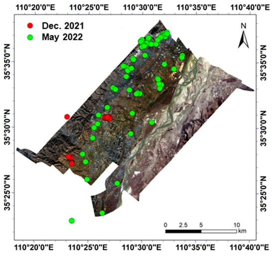
Figure 3.
Geographical location of sampling points with airborne-based hyperspectral imagery in the Hancheng mining areas.
Examples of ground photos reflecting soil status in two campaigns are shown in Figure 4. The sampled soils were properly labeled for laboratory analysis. Soil-related HM parameters (including Cu, Pb, Zn, Ni, Cr, Cd, As, and Hg) were measured by the Shanxi Geophysical and Chemical Exploration Institute Co., Ltd. (located in Yuncheng, China). The laboratory environments for measuring MHs include a temperature range of 18–26 °C, humidity levels between 41 and 49%RH%, and standard atmospheric pressure. The main instruments include the analytical balance (AUY-120), the inductively coupled plasma optical emission spectroscopy (ICP-OES), the fully automatic double-channel atomic fluorescence spectrometer (AFS-230E), and the high-performance atomic absorption spectrometer (ZEEnit650P). Note that soil-related HM parameters will be further explored in Section 3.2.
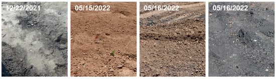
Figure 4.
Examples of ground photos reflecting varied soil status.
2.3. Methods
2.3.1. Methodology Overview
The framework of soil-related parameter modeling methodology is presented in Figure 5 and encompasses four steps (field measurements, data preprocessing, spectral analysis and soil-related parameter modeling, and accuracy estimation and HM concentration mapping) as follows:
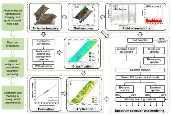
Figure 5.
The framework of the soil-related parameter estimate method.
- Step 1: Airborne-based hyperspectral imagery, ASD soil reflectance, and soil-related HM concentrations were collected and measured as original data, described in detail in Section 2.2.
- Step 2: Data preprocessing includes both airborne-based imagery and ground-based field observations. Geometric corrections, radiometric calibration, atmospheric correction, and region of interest (ROI) extraction were conducted using airborne-based imagery. The data pruning process was performed on the ground-based soil samples.
- Step 3: Select high-quality and soil-related parameter response characteristics wavelengths from ground-based ASD and airborne-based spectral reflectance. The soil-related parameter modeling process is based on ML methods using the 428 hyperspectral wavelength selection results.
- Step 4: Evaluation metrics were used to estimate the accuracy between predicted HM concentrations and ground truth in situ data, and then the best performance model was selected to map the HM concentrations in the whole region.
The details of the steps in the flowchart are described in the following subsections.
2.3.2. Data Preprocessing
For airborne-based imagery, geometric corrections, radiometric calibration, and atmospheric correction, there are three important preprocessing steps for avoiding radiometric errors and removing geometric distortion and the effects of the atmosphere. Firstly, the flight attitude (roll, pitch, and yaw) can cause geometric errors when using an AMMIS push broom scanner to acquire airborne-based hyperspectral imagery [31,32]. Ground control points (GCPs) were used for the geometric correction of high-resolution airborne-based imagery. The real-time kinematic (RTK) technique was used to obtain the coordinates of all GCPs. Secondly, the gain and offset coefficients needed in the radiometric calibration process were obtained from four different grayscale artificial targets (5%, 20%, 40%, and 60%) (as shown in Figure 2a). These calibration coefficients were fitted using the digital number (DN) and radiance of the airborne sensor modeled by synchronous measurement of these target reflectance and atmospheric parameters (including AOD and CWV), which were obtained by the CE318. Finally, the fast line-of-sight atmospheric analysis of spectral hypercubes (FLAASH) module was used to make the atmospheric correction for the whole imagery. According to the geographic locations of ground-based soil samples (as shown in Figure 3), a sub-region area that covered the mining area and had potential HMs in the soil was selected as the study area from the airborne-based image (as shown in Figure 6a).
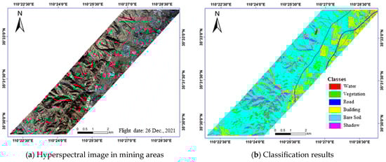
Figure 6.
The airborne-based hyperspectral image and corresponding classification results. (a) The hyperspectral imagery displayed with a true color combination; (b) Classification results of the corresponding area.
Based on the above results, the maximum likelihood classification algorithm [33,34] was applied to the preprocessed hyperspectral image and generated six clusters, including water, vegetation, road, building, bare soil, and shadow. The classification results of six types of land cover are shown in Figure 6b. The largest proportion of land cover classification is bare soil, accounting for 62.0%. It is followed by the building class, at 21.30%. The percentages of water, vegetation, road, and shadow classes are 0.19%, 7.36%, 2.54%, and 6.64%, respectively. The shadow areas are caused by the three-dimensional (3D) structures of mountains and buildings. Then, the classification results were used to eliminate non-bare soil pixels in the hyperspectral image, and in the application (detailed in Section 4.2), the concentrations of HMs in this study area were mapped through the proposed model.
In addition, for the ground-based data preprocessing, the original number of soil samples is 100. However, there are two soil sample points outside the flight area, and the number of input soil samples is 98. Then, the ground-based field and airborne-based data pruned high-value samples, respectively, and finally formed the preprocessing data results.
2.3.3. Machine Learning Methods
In the hyperspectral inversion study, three well-known ML methods, including RF [35], SVM [36], and PLS [37], are commonly used and have been successfully applied to predict soil-related parameters. For example, based on ASD hyperspectral data, Tan et al. [21] used these three methods to establish an estimation model for four kinds of HMs and showed that the RF method was superior to the PLS and SVM methods. Pandit et al. [25] used the PLS method to predict and map the spatial distribution of Pb based on ASD hyperspectral data. However, most of the existing studies are based on the ground spectra [11]. There have been very few studies on simultaneous and integrated airborne–ground hyperspectral data. Therefore, based on comprehensive observations, this study explored PF, SVM, and PLS methods to establish high-performance soil-related parameter estimation models. These models were performed with the Python ‘sklearn’ library [38]. With regard to dataset splitting, 70% of the soil samples were used for training, and 30% were for testing. A brief introduction to each and their detailed parameters are as follows:
- RF is an ensemble learning method based on the bagging technique (or bootstrap aggregation) [39] used for both classification and regression analysis. The RF method is a robust predictor for both small sample sizes and high-dimensional data [40]. In this study, the RF method was used to build the soil-related parameter regression models, running in default mode with automated parameter tuning and 1000 trees in the forest, with the number of the random-state parameter set to 1.
- SVM is a supervised learning technique that has been successfully applied for classification and regression based on various kernels, such as the linear, polynomial, sigmoid, and radial basis function (RBF) kernels [41]. This study focuses on the SVM method with the RBF kernel due to its effectiveness, as confirmed by previous studies [42,43,44]. The regularization parameter C and the kernel coefficient (gamma) mode were set to 1.0 and ‘Auto’, respectively.
- PLS is a multivariate regression method that aims to find a few components or latent variables that are linear combinations of explanatory variables based on the covariance structure [45]. In this study, the PLS was used to establish the relationship between the reflectance spectra and soil-related HM concentrations in default parameters with three components to keep.
In the soil-related parameter modeling processes, the RF, SVM, and PLS regression models were trained based on airborne- and ground-based data, including the soil reflectance data of 428 hyperspectral bands and HM concentrations of soil samples. The detailed modeling processes for the training and testing stages are presented in the following part.
2.3.4. Spectral Analysis and Soil-Related Parameter Modeling
Spectral analysis is based on spectral resampling and spectral envelope methods. This study uses the airborne-based hyperspectral bands as the spectral library in the spectral resampling process. The ground-based soil spectra were automatedly resampled to match the bands in the airborne-based spectral library. Moreover, the spectral envelope method is referred to as continuum removal or convex hull transform. The continuum is a convex hull fitted over the top of a spectrum and is constructed by connecting local spectra maxima using straight line segments [46]. The spectral envelope process is represented in Equation (1).
where R′ means continuum-removed soil spectra, R is the original soil reflectance values, and Rc is the soil reflectance values of the continuum curve. The resulting spectral curves have values between 0 and 1. These preprocessed spectra are analyzed for building soil-related parameter estimation models.
R′ = R/Rc,
Let be the preprocessed soil spectral reflectance data in the B band associated with a location in the soil samples. When all soil samples are combined, it can be represented with an matrix denoted as X,
where the rows (1, 2, …, n) are associated with soil sample locations, and columns (1, 2, …, B) are associated with the number of bands.
In summary, the ground- and airborne-based preprocessed soil samples are denoted as GS, GCS, AS, and ACS; the ground- and airborne-based preprocessed spectral reflectance are denoted as GRR, GER, AOR, and AER, respectively. Table 2 illustrates the input data in the combination of soil spectral reflectance and the HM concentrations of each soil sample. Three ML methods were tested in combination with these eight data subsets.
Table 2.
The detailed description and explanation of the input data subsets.
2.3.5. Evaluation Metrics
Three evaluation metrics, including the coefficient of determination (R2), the root-mean-squared error (RMSE), and relative prediction deviation (RPD), were used to evaluate the accuracy of the soil-related parameter regression models. The R2 metric denotes the squared correlation between the measured HMs’ concentrations (ground truth) and the predicted values, which varies from 0.0 (no linear relationship) to 1.0 (perfect correlation). In addition, the RMSE metric denotes the average difference between the in situ concentration of eight types of HMs and predicted values, which was calculated by the Scikit-learn metrics module in Python 3.9 [38] in the training and testing stages. The RPD is the ratio of the sample standard deviation to the RMSE, which was used to evaluate the model’s prediction performance. According to one previous study [47], the RPD values can be grouped into three categories, as follows: RPD < 1.4 means the predictions are not recommended; RPD values between 1.4 and 2.0 indicate fair predictions; and RPD > 2.0 denotes excellent predictions. Moreover, a previous study [48] divided the 1.4 and 2.0 intervals as follows: RPD values between 1.4 and 1.8 indicate fair predictions, and values between 1.8 and 2.0 indicate good predictions. The R2, RMSE, and RPD metrics are defined by the following Equations (4), (5), and (6), respectively.
where, n is the number of soil samples, is the measured ground truth HMs concentrations of the soil sample i, is the predicted HMs concentrations of the corresponding soil sample, and is the average measured HMs concentrations. SD presents the standard deviation of the predicted concentrations.
3. Results
3.1. Soil Spectrum Selection Results
Along with integrated ground–airborne observation systems, the ASD spectroradiometer and airborne-based hyperspectral remote sensing data from the sampling sites were used to generate the variability in individual reflectance curves for each soil sample. The analysis results regarding the similarities and differences across measurements from the ASD and airborne-based spectra are as follows:
- Ground-based in situ soil reflectance spectra: The reflectance spectra in the range of 400 nm to 2500 nm of 100 soil samples measured by the ground-based ASD spectroradiometer were resampled to the corresponding wavelengths of the AMMIS through the response function. As shown in Figure 7a, soil samples’ in situ resampling reflectance characteristics show various fluctuations across the full spectral range. For example, in the wavelength ranges of 400–1200 nm, 1450–1750 nm, and 2000–2300 nm, the spectral reflectance values of entire soil samples are between 0 and 0.6, with a smoother trend than other ranges across the full spectra. In contrast, three strong reflectance variations were formed near 1400 nm, 1900 nm, and 2400 nm, and two absorption valleys were observed near 2200 nm and 2300 nm. The absorption features in the infrared region are usually narrower and sharper than in the VIS channel. There are several reasons for these reflective characteristics. The atmospheric CWV, the SNR of the ASD instrument, and its systematic errors affect the measurement results regarding soil reflectance. In addition, the absorption peaks near 1400 and 1900 nm are strongly associated with the bending and stretching of the hydroxyl (OH) features of hygroscopic or free water [49,50]. Combination vibrations involving the metal–OH bending and OH stretching occur in the 2200–2500 nm region [51]. These soil spectral features are consistent with previous studies [49,50,51,52,53,54]. Generally, the reflectance differences across all soil samples are obvious, and the characteristic bands of soil-related parameter concentrations are mainly focused on the NIR and SWIR channels.
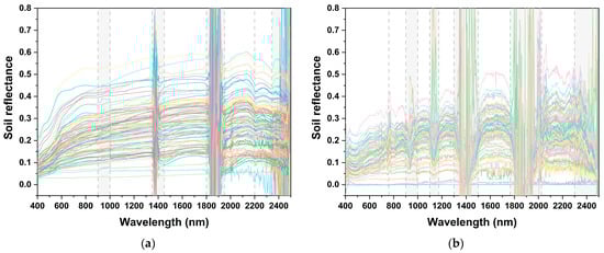 Figure 7. Soil reflectance spectra of all samples. (a) Soil reflectance characteristics measured by the ground-based ASD spectroradiometer; (b) soil reflectance characteristics extracted from the airborne-based hyperspectral remote sensing imagery. The obvious fluctuations of soil reflectance in the full spectral ranges are indicated with gray blocks.
 - Airborne-based soil reflectance spectra: According to the in situ geographic location of each soil sample, soil reflectance spectra were extracted from the airborne-based hyperspectral remote sensing images (as shown in Figure 7b). There are similarities and differences in the shape and value of spectral curves between ground- and airborne-based soil spectral reflectance characteristics. Generally, the airborne-based soil reflectance spectra were rougher than the ground-based measurements, with more obvious variations between 400 nm and 2500 nm. For example, five strong reflectance spectral variations were observed near 950 nm, 1150 nm, 1400 nm, 1900 nm, and 2300 nm. The reasons for the three strong reflectance variations near 1400 nm, 1900 nm, and 2300 nm were similar to those influencing the ground-based in situ reflectance spectra. In addition, oxygen (O2) has well-known atmospheric absorption bands in the VNIR spectrum near 760 nm [55]. In addition, the radiometric calibration, atmospheric correction errors of airborne-based hyperspectral data, geographical spatial matching, and heterogeneity also influence the soil spectral characteristics.
In summary, according to ground-based ASD and airborne-based data, in the spectral curves, variations in the overall reflectance intensity and absorption bands and changes in the spectral shape were observed; the ground-based soil reflectance and airborne-based soil reflectance showed some similarities and differences in spectral characteristics. There are some negative reflectance values due to noise in the measurements and low signals reaching dark signal levels. Considering the high-quality data and obvious spectral characteristics, five wavelength ranges out of the four hundred and twenty-eight bands were selected to explore the relationship between soil reflectance spectra and soil-related parameter data. These ranges were 437.1–864.24 nm, 993.32–1079.92 nm, 1175.52–1298.82 nm, 1529.73–1747.52 nm, and 2080.64–2393.26 nm.
3.2. Analysis of the Concentrations of Eight Heavy Metal(loid)s
Figure 8 displays the ground-measured Cu, Pb, Zn, Ni, Cr, Cd, As, and Hg concentrations in 100 soil samples. In all samples, the mean values (mg/kg) of the above eight HMs’ content are 25.88, 23.11, 73.15, 28.79, 57.03, 0.13, 10.99, and 0.07, respectively. Zn content is the highest of all the metals shown and has more than doubled along with that of Cu, Pb, and Ni. The Ni and Cr elements present relatively high concentrations compared to Cu, Pb, Cd, As, and Hg. In spite of Cd and Hg’s low abundance, the extensive use of Hg and Cd has led to significant soil contamination and has sometimes resulted in toxic levels of exposure for humans and animals [3].
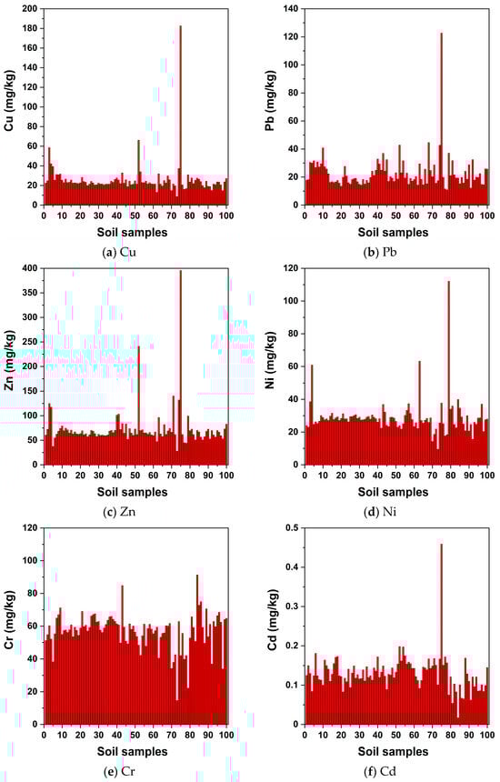
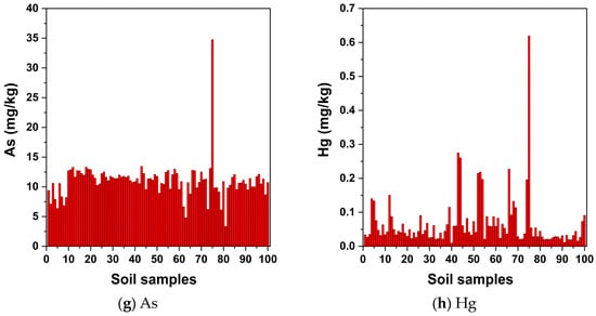
Figure 8.
Numerical distribution of eight soil-related parameters in soil samples.
Below are some detailed distributions among the concentrations of each HM. The concentrations of Cu vary from 8.74 mg/kg to 182.6 mg/kg, with a central range from 20 mg/kg to 30 mg/kg. The high-frequency values of Pb content range from 15 mg/kg to 30 mg/kg, and the maximum and minimum contents are 122.65 mg/kg and 10.95 mg/kg, respectively. The maximum and minimum contents of Zn are 27.74 mg/kg and 395.45 mg/kg, respectively, but most samples contain 50–75 mg/kg. The maximum and minimum contents of the Ni are 112.11 mg/kg and 9.55 mg/kg, respectively, and the distribution center is between 20 mg/kg and 30 mg/kg. The maximum and minimum values of Cr are 91.32 mg/kg and 14.63 mg/kg, respectively, with the majority of content values concentrated between 40.0 mg/kg and 60.0 mg/kg. The majority of As content values fall within the range of 7.0 mg/kg to 13.0 mg/kg, with the maximum and minimum values recorded at 34.76 mg/kg and 3.35 mg/kg, respectively. The contents of Cd and Hg are relatively lower than those of other HMs. The maximum contents of Cd and Hg are 0.46 mg/kg and 0.62 mg/kg, respectively. Their minimum contents are 0.02 mg/kg and 0.01 mg/kg, respectively. The high-frequency values of Cd and Hg contents vary from 0.08 mg/kg to 0.15 mg/kg and from 0.03 mg/kg to 0.10 mg/kg. In the previous study [3], the concentrations of HMs have two aspects: from a geochemical perspective, the HMs are normally found in rocks and soils with concentrations below 1000 mg/kg (except for natural concentrations in ore minerals that form ore deposits). In contrast, biology defines the concentrations at relatively low values, typically below 100 mg/kg, in the dry matter of living organisms.
Hence, it can be concluded that the concentrations of the eight HMs are relatively low values and are evenly distributed across the soil samples. However, one or two anomalously high concentration values of the eight soil-related HMs were observed compared with the corresponding mean values. For example, the highest content values of six HMs, including Cu, Pb, Zn, Cd, As, and Hg, were all measured in the No. 75 soil sample. The highest Ni and Cr content values were observed in soil samples No. 79 and No. 84, respectively.
3.3. Soil-Related Parameter Modeling Results
The eight combination subsets of soil samples and spectral reflectance values from both ground and airborne platforms, including GRR-GS, GRR-GCS, GER-GS, GER-GCS, AOR-AS, AOR-ACS, AER-AS, and AER-ACS (refer to Table 2 for details regarding the acronyms), were fed into the three regression methods (RF, SVM, and PLS) as the input data. Table 3 shows the RMSE accuracy estimation results in three methods’ training and testing stages with the eight input data subsets. The RF method yielded higher performance than the SVM and PLS methods in all combination data subsets and obtained lower RMSE values with the GER-GCS and AER-ACS subsets than other combination datasets. Their average RMSE values are 2.53 and 2.61 mg/kg, respectively. The RF method with the GER-GCS ground-based data subsets exhibited the highest accuracy in Pb and Ni estimations, and the RMSE values were 2.07 and 2.48, respectively. The predicted Cu, Zn, and Cr concentrations were most accurately retrieved using the RF method with the airborne-based data subsets (AER-ACS and AOR-ACS) with RMSE values of 1.87, 8.17, and 3.17 mg/kg, respectively. For three HMs (Cd, As, and Hg), the RF method using the GER-GCS and AER-ACS data subsets had equal RMSE values at 0.01, 0.69, and 0.02, respectively.
Table 3.
Evaluation of soil-related HM parameter modeling results based on eight ground- and airborne-based data subsets. The best models and the minimum RMSE values of each HM parameter are highlighted.
Whether using airborne- or ground-based datasets, after eliminating high-value samples (the GCS and ACS datasets), the accuracy of different methods was improved, especially in the cases of four soil-related parameters (Cu, Pb, Zn, and Ni). The main reason is that there are only one or two samples with high-value soil-related parameters across the 100 samples. The regression processes in the three methods relied on most non-high-value samples. Thus, the high RMSE values were yielded in estimating the minority of high-value soil-related parameters.
Moreover, the RMSE values of the three methods with pruned and envelope data subsets (GER-GCS and AER-ACS) were less than those of unpruned and non-envelope data subsets. The main reason is that the envelope method emphasizes the spectral shape characteristics and strengthens the role of the characteristic bands. Taking the RF method and two combination data subsets (GER-GCS and GRR-GCS) as examples, the estimation results demonstrate that the Pb and Zn contents retrieved using GER-GCS were more accurate than those obtained from GEE-GCS, with increases of 0.46 and 1.04, respectively.
In summary, the RF method using the GER-GCS and AER-ACS data subsets achieved high performance in the soil-related parameter retrieval models’ training and testing stages, and the optimal ground- and airborne-based regression models were denoted as GER-GCS-RF and AER-ACS-RF, respectively.
4. Discussion
4.1. Transferability of Soil-Related Parameter Retrieval Models
Based on the evaluation results of three ML methods within the eight combinations of soil data subsets, the best ground- and airborne-based regression models were defined as GER-GCS-RF and AER-ACS-RF, respectively. In order to test the predictive transferability of the ground-based regression model (GER-GCS-RF), the AER-ACS and AER-AS combination data subsets were used as the input spectral data, and the predictive results from the model were compared with the ground truth contents of the eight HMs.
Figure 9 shows the RMSE (mg/kg) evaluation results. In general, the RMSE values of the ground-based GER-GCS-RF model with the AER-ACS and AER-AS data subsets were higher than the airborne-based AER-ACS-RF model with the corresponding data subsets, which revealed that the ground-based model had certain limitations in airborne-based transferability applications. For example, in the estimation results of Zn, the ground-based GER-GCS-RF model with the airborne-based AER-AS data subset revealed less transferability, with the highest RMSE value of 42.326 mg/kg. Due to the ground- and airborne-based sensors’ characteristics, the transferability differences were obvious in the testing results. In Figure 7, the specific differences in spectral characteristics between ground- and airborne-based soil reflectance are shown.
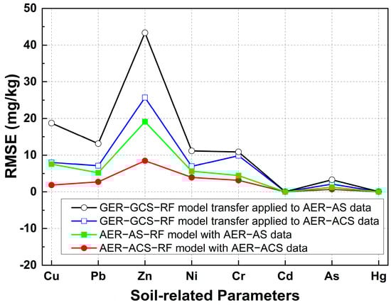
Figure 9.
Transferability evaluation results of ground- and airborne-based RF models.
In addition, as shown in Figure 10, the best AER-ACS-RF model was evaluated on the R2 metric between the ground truth and the predicted contents of the eight HMs. The highest R2 values were observed in Cd and As, with an equal value of 0.98. These were followed by Pb (R2 = 0.97). The evaluation model with the Cr and Hg soil-related parameters yielded the same fitting performance, with an equal R2 value of 0.95. The R2 value between the predicted contents and the measured values of Cu was 0.92. The R2 scores of Zn and Ni were relatively low among the eight soil-related parameters, with R2 values of 0.88 and 0.79, respectively. Overall, the linear fitting results of R2 values between the predicted contents and the ground truth data were generally relatively high, with five of the eight soil-related parameters’ R2 scores being above 0.95.
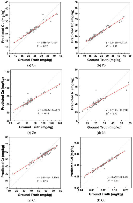
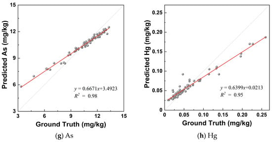
Figure 10.
Soil parameter estimation results from an airborne envelope random forest model compared with ground measurements.
Moreover, the RPD metric was used to evaluate the performance of the retrieval model. The RPD values of Cu and As were 1.94 and 1.93, respectively. According to the RPD categories, these values indicated good predictions by the retrieval model. The RPD values of Pb (1.73), Cr (1.69), Cd (1.66), and Hg (1.69) were between 1.4 and 1.8, which indicated fair predictions. Similar to the ranking of the R2 scores of Zn and Ni among the eight HMs, their RPD values were also relatively low, at 1.25 and 1.19, respectively. Upon examining the fitting metric of the eight soil-related parameters, the AER-ACS-RF model tended to underestimate the high-value contents and overestimate the low-value contents of each HM. There are two factors that may contribute to the predicted performance. The effect of the retrieval model can only partially explain the observations. The high and low HM concentrations have certain uneven distributions in the soil samples. Therefore, the universal model can be further explored, and the number of soil samples should be expanded in field measurements.
4.2. Mapping the Estimated Concentrations in Real Application
Based on the airborne-based hyperspectral imagery, the real application of mapping the contents of HMs in the Hancheng mining areas was conducted using the best airborne-based retrieval model (AES-ACS-RF) to predict them in bare soil pixels and panoramic pixels. Figure 11(a1–h1) shows the mapping results in bare soil pixels with eight HM concentrations, while Figure 11(a2–h2) presents the predicted results in panoramic pixels.

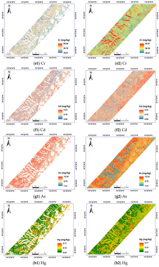
Figure 11.
Mapping results of spatial distributions of the eight HMs in bare soil pixels (left) and panoramic pixels (right).
For the mapping results in bare soil pixels, the high-value contents of the six HMs, including Cu, Pb, Zn, Cr, Cd, and As, were generally distributed in mining areas, while the relatively low-value contents were observed in farmland areas. A strong spatial correlation was observed between the estimated contents of these six HMs. In the histogram statistical results (as shown in Figure 12a–h), the maximum predicted concentrations of Cu, Pb, Zn, Ni, Cr, Cd, As, and Hg were 31.25, 30.45, 109.48, 32.47, 66.56, 0.23, 12.24, and 0.17 mg/kg, respectively. The minimum concentrations of these eight HMs were 21.65, 16.38, 62.02, 23.33, 49.81, 0.09, 7.31, and 0.03 mg/kg, respectively. The majority of the predicted concentrations of three HMs (Cu, Pb, and Ni) were relatively close, ranging from 22.0 mg/kg to 26.0 mg/kg, 18.0 mg/kg to 24.0 mg/kg, and 26.0 mg/kg to 30.0 mg/kg, respectively. The high-frequency concentration ranges of Zn and Cr were 60.0–80.0 mg/kg and 53.0–62.0 mg/kg, respectively. Most of the predicted concentrations of As ranged from 9.0 mg/kg to 11.5 mg/kg. Similar to the ground truth distributions, the estimated concentrations of Cd and Hg were lower than those of other HMs. Their high-frequency values spanned from 0.12 mg/kg to 0.14 mg/kg and from 0.02 mg/kg to 0.12 mg/kg, respectively.
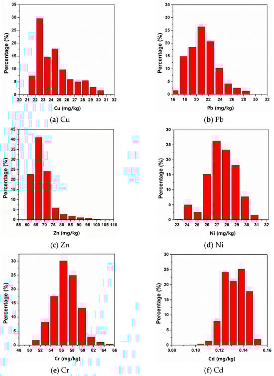
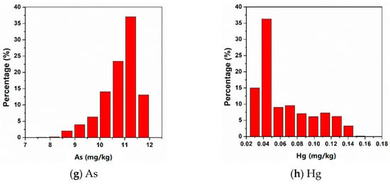
Figure 12.
Numerical histogram of the predicted contents of eight soil parameters in bare soil pixels.
Unlike the mapping results in the bare soil pixels, the highest predicted concentrations of Cu (Figure 11(a2)), Pb (Figure 11(b2)), and Cr (Figure 11(e2)) were observed in the shadow and water pixels, while the lowest predicted concentrations of Cd (Figure 11(f2)) and As (Figure 11(g2)) were observed in the corresponding areas. Note that the airborne hyperspectral data used in this study were characterized by high spatial resolution (VNIR: 0.25 m and SWIR: 0.5 m). Therefore, the influence of mixed pixels was not considered. These predicted results in the panoramic pixels show significant differences compared to the ground truth values. Due to the uncertainty in the reflectance of shadow pixels, there is a certain error in the inversion results of the panoramic pixels. Therefore, according to the above mapping results in the different land cover types, this study recommends using the predicted results retrieved from bare soil pixels.
5. Conclusions
This study aimed to estimate and predict soil quality parameters in mining areas in the FWP, leveraging ground-based in situ measurements and airborne-based hyperspectral imagery within three ML methods. Ground- and airborne-based inversion models of eight soil quality parameters, including Cu, Pb, Zn, Ni, Cr, Cd, As, and Hg, were trained and tested with eight combination data subsets (GRR-GS, GRR-GCS, GER-GS, GER-GCS, AOR-AS, AOR-ACS, AER-AS, and AER-ACS) based on spectral resampling and envelope methods.
- The integrated airborne–ground remote sensing observation experiments were conducted in the FWP region. Based on collected in situ soil-related parameters and hyperspectral soil reflectance, five wavelength ranges out of four hundred and twenty-eight bands were selected to explore the relationship between soil reflectance spectra and soil-related parameter data, which were 437.1–864.24 nm, 993.32–1079.92 nm, 1175.52–1298.82 nm, 1529.73–1747.52 nm, and 2080.64–2393.26 nm.
- Eight data combination subsets were fed into three ML methods for training and testing the soil-related parameters. The best performance model within the corresponding data subset was defined. The accuracy of the RF method with the airborne-based data subset (AER-ACS-RF model) in predicting the eight soil-related parameters surpasses the other two methods (SVM and PLS) within other seven data subsets, with evaluation values of R2 = 0.92, RMSE = 1.87 mg/kg, and RPD = 1.94 for Cu; R2 = 0.97, RMSE = 2.74 mg/kg, and RPD = 1.73 for Pb; R2 = 0.88, RMSE = 8.47 mg/kg, and RPD = 1.25 for Zn; R2 = 0.79, RMSE = 3.92 mg/kg, and RPD = 1.19 for Ni; R2 = 0.95, RMSE = 3.17, and RPD = 1.69 for Cr; R2 = 0.98, RMSE = 0.01 mg/kg, and RPD = 1.66 for Cd; R2 = 0.98, RMSE = 0.69 mg/kg, and RPD = 1.93 for As; and R2 = 0.98, RMSE = 0.02 mg/kg, and RPD = 1.69 for Hg.
- In the real application, the optimal airborne-based model (AER-ACS-RF) was used to estimate and map the contents of the eight soil-related parameters in Hancheng mining area, ranging from 21.65 to 31.25 (Cu), 16.38 to 30.45 (Pb), 62.02 to 109.48 (Zn), 23.33 to 32.47 (Ni), 49.81 to 66.56 (Cr), 0.09 to 0.23 (Cd), 7.31 to 12.24 (As), and 0.03 to 0.17 (Hg), respectively, which revealed the spatial characteristics between these parameters.
However, due to the certain differences between in situ-measured soil spectra and airborne-based hyperspectral data, the ground-based model had limitations in transferability applications to airborne-based data. The highest RMSE value in the transferability evaluation was observed for Zn. In addition, although this study has discussed the effect of the types of land cover between bare soil pixels and others (water, vegetation, road, building, and shadow pixels) and suggests that the AER-ACS-RF model is beneficial for bare soil land cover, there is a need to explore the optimal algorithm for retrieving the parameters in full land cover types, which would be helpful for developing a comprehensive understanding of the status of soil pollution and to provide a global reference for soil environmental quality monitoring. Thus, the establishment of effective estimating and monitoring methods for soil-related parameters remains a long-term challenge, especially leveraging airborne- and ground-based hyperspectral data captured from simultaneous and integrated remote sensing observations.
Author Contributions
Conceptualization, C.J. and H.R.; methodology, C.J. and H.R.; validation, Z.W. and H.Z. (Hui Zeng); investigation and data curation, H.Z. (Hui Zeng), Y.T., H.Z. (Hongqin Zhang), X.L., D.J. and M.W.; resources, R.L.; writing—original draft preparation, C.J.; writing—review and editing, H.R. and Z.W.; visualization, B.W. and J.Z.; funding acquisition, H.R. All authors have read and agreed to the published version of the manuscript.
Funding
This research was supported by the National Science and Technology Major Project of China (04-H30G01-9001-20/22), the Outstanding Youth Program of the National Natural Science Foundation of China (42222107), and the National Civil Aerospace Project of China (D040102).
Data Availability Statement
The soil sample data that support the findings of this study are available from the corresponding author, renhuazhong@pku.edu.cn, upon reasonable request and scientific research needs.
Acknowledgments
The authors would like to thank the Hebei Provincial Prospecting Institute of Hydrogeology and Engineering Geology for their work on the field measurements and laboratory processing of soil samples and the Shanxi Geophysical and Chemical Exploration Institute Co., Ltd., which acquired and processed the HMs contents.
Conflicts of Interest
The authors declare no conflicts of interest.
References
- Gardi, C.; Jeffery, S.; Saltelli, A. An estimate of potential threats levels to soil biodiversity in EU. Glob. Chang. Biol. 2013, 19, 1538–1548. [Google Scholar] [CrossRef] [PubMed]
- FAO; ITPS. Status of the World’s Soil Resources (SWSR): Main Report; Food and Agriculture Organization of the United Nations and Intergovernmental Technical Panel on Soils: Rome, Italy, 2015. [Google Scholar]
- Alloway, B.J. Heavy Metals in Soils: Trace Metals and Metalloids in Soils and their Bioavailability, 3rd ed.; Springer Science & Business Media: Dordrecht, The Netherlands, 2012; pp. 241–493. [Google Scholar]
- Zhao, H.; Wu, Y.; Lan, X.; Yang, Y.; Wu, X.; Du, L. Comprehensive assessment of harmful heavy metals in contaminated soil in order to score pollution level. Sci. Rep. 2022, 12, 3552. [Google Scholar] [CrossRef] [PubMed]
- Liu, W.; Yu, Y.; Li, M.; Yu, H.; Shi, M.; Cheng, C.; Hu, T.; Mao, Y.; Zhang, J.; Liang, L.; et al. Bioavailability and regional transport of PM2.5 during heavy haze episode in typical coal city site of Fenwei Plain, China. Environ. Geochem. Health 2023, 45, 1933–1949. [Google Scholar] [CrossRef] [PubMed]
- Maus, V.; Giljum, S.; da Silva, D.M.; Gutschlhofer, J.; da Rosa, R.P.; Luckeneder, S.; Gass, S.L.B.; Lieber, M.; McCallum, I. An update on global mining land use. Sci. Data 2022, 9, 433. [Google Scholar] [CrossRef] [PubMed]
- Bioucas-Dias, J.M.; Plaza, A.; Camps-Valls, G.; Scheunders, P.; Nasrabadi, N.; Chanussot, J. Hyperspectral Remote Sensing Data Analysis and Future Challenges. IEEE Geosci. Remote Sens. Mag. 2013, 1, 6–36. [Google Scholar] [CrossRef]
- Pour, A.B.; Zoheir, B.; Pradhan, B.; Hashim, M. Editorial for the Special Issue: Multispectral and Hyperspectral Remote Sensing Data for Mineral Exploration and Environmental Monitoring of Mined Areas. Remote Sens. 2021, 13, 519. [Google Scholar] [CrossRef]
- Bishop, C.A.; Liu, J.G.; Mason, P.J. Hyperspectral remote sensing for mineral exploration in Pulang, Yunnan Province, China. Int. J. Remote Sens. 2011, 32, 2409–2426. [Google Scholar] [CrossRef]
- Notesco, G.; Kopačková, V.; Rojík, P.; Schwartz, G.; Livne, I.; Dor, E.B. Mineral Classification of Land Surface Using Multispectral LWIR and Hyperspectral SWIR Remote-Sensing Data. A Case Study over the Sokolov Lignite Open-Pit Mines, the Czech Republic. Remote Sens. 2014, 6, 7005–7025. [Google Scholar] [CrossRef]
- Tan, K.; Ma, W.; Chen, L.; Wang, H.; Du, Q.; Du, P.; Yan, B.; Liu, R.; Li, H. Estimating the distribution trend of soil heavy metals in mining area from HyMap airborne hyperspectral imagery based on ensemble learning. J. Hazard. Mater. 2021, 401, 123288. [Google Scholar] [CrossRef]
- Farrand, W.H.; Harsanyi, J.C. Mapping the distribution of mine tailings in the Coeur d’Alene River Valley, Idaho, through the use of a constrained energy minimization technique. Remote Sens. Environ. 1997, 59, 64–76. [Google Scholar] [CrossRef]
- Choe, E.; van der Meer, F.; van Ruitenbeek, F.; van der Werff, H.; de Smeth, B.; Kim, K.-W. Mapping of heavy metal pollution in stream sediments using combined geochemistry, field spectroscopy, and hyperspectral remote sensing: A case study of the Rodalquilar mining area, SE Spain. Remote Sens. Environ. 2008, 112, 3222–3233. [Google Scholar] [CrossRef]
- Wu, Y.; Zhang, X.; Liao, Q.; Ji, J. Can Contaminant Elements in Soils Be Assessed by Remote Sensing Technology: A Case Study With Simulated Data. Soil Sci. 2011, 176, 196–205. [Google Scholar] [CrossRef]
- Kruse, F.; Boardman, J.; Lefkoff, A.; Young, J.; Kierein-Young, K.; Cocks, T.; Jensen, R.; Cocks, P. HyMap: An Australian hyperspectral sensor solving global problems-results from USA HyMap data acquisitions. In Proceedings of the 10th Australasian Remote Sensing and Photogrammetry Conference, Adelaide, Australia, 21–25 August 2000; pp. 18–23. [Google Scholar]
- Green, R.O.; Eastwood, M.L.; Sarture, C.M.; Chrien, T.G.; Aronsson, M.; Chippendale, B.J.; Faust, J.A.; Pavri, B.E.; Chovit, C.J.; Solis, M.; et al. Imaging Spectroscopy and the Airborne Visible/Infrared Imaging Spectrometer (AVIRIS). Remote Sens. Environ. 1998, 65, 227–248. [Google Scholar] [CrossRef]
- Wang, F.; Gao, J.; Zha, Y. Hyperspectral sensing of heavy metals in soil and vegetation: Feasibility and challenges. ISPRS J. Photogramm. Remote Sens. 2018, 136, 73–84. [Google Scholar] [CrossRef]
- Dai, X.; Wang, Z.; Liu, S.; Yao, Y.; Zhao, R.; Xiang, T.; Fu, T.; Feng, H.; Xiao, L.; Yang, X.; et al. Hyperspectral imagery reveals large spatial variations of heavy metal content in agricultural soil—A case study of remote-sensing inversion based on Orbita Hyperspectral Satellites (OHS) imagery. J. Clean. Prod. 2022, 380, 134878. [Google Scholar] [CrossRef]
- Liu, Z.; Lu, Y.; Peng, Y.; Zhao, L.; Wang, G.; Hu, Y. Estimation of Soil Heavy Metal Content Using Hyperspectral Data. Remote Sens. 2019, 11, 1464. [Google Scholar] [CrossRef]
- Tan, K.; Wang, H.; Chen, L.; Du, Q.; Du, P.; Pan, C. Estimation of the spatial distribution of heavy metal in agricultural soils using airborne hyperspectral imaging and random forest. J. Hazard. Mater. 2020, 382, 120987. [Google Scholar] [CrossRef]
- Tan, K.; Ma, W.; Wu, F.; Du, Q. Random forest–based estimation of heavy metal concentration in agricultural soils with hyperspectral sensor data. Environ. Monit. Assess. 2019, 191, 446. [Google Scholar] [CrossRef] [PubMed]
- Jia, J.; Chen, J.; Zheng, X.; Wang, Y.; Guo, S.; Sun, H.; Jiang, C.; Karjalainen, M.; Karila, K.; Duan, Z.; et al. Tradeoffs in the Spatial and Spectral Resolution of Airborne Hyperspectral Imaging Systems: A Crop Identification Case Study. IEEE Trans. Geosci. Remote Sens. 2022, 60, 5510918. [Google Scholar] [CrossRef]
- Wu, Y.Z.; Chen, J.; Ji, J.F.; Tian, Q.J.; Wu, X.M. Feasibility of Reflectance Spectroscopy for the Assessment of Soil Mercury Contamination. Environ. Sci. Technol. 2005, 39, 873–878. [Google Scholar] [CrossRef]
- Choe, E.; Kim, K.-W.; Bang, S.; Yoon, I.-H.; Lee, K.-Y. Qualitative analysis and mapping of heavy metals in an abandoned Au–Ag mine area using NIR spectroscopy. Environ. Geol. 2009, 58, 477–482. [Google Scholar] [CrossRef]
- Pandit, C.M.; Filippelli, G.M.; Li, L. Estimation of heavy-metal contamination in soil using reflectance spectroscopy and partial least-squares regression. Int. J. Remote Sens. 2010, 31, 4111–4123. [Google Scholar] [CrossRef]
- Zhao, Z.; Liu, R.; Zhang, Z. Characteristics of Winter Haze Pollution in the Fenwei Plain and the Possible Influence of EU During 1984–2017. Earth Space Sci. 2020, 7, e2020EA001134. [Google Scholar] [CrossRef]
- Zhang, B.; Shen, Z.; Sun, J.; Zhang, L.; He, K.; Zhang, Y.; Xu, H.; Lv, J.; Cao, L.; Li, J.; et al. County-level and monthly resolution multi-pollutant emission inventory for residential solid fuel burning in Fenwei Plain, China. Environ. Pollut. 2023, 330, 121815. [Google Scholar] [CrossRef]
- Lin, C.; Huang, R.J.; Zhong, H.; Duan, J.; Wang, Z.; Huang, W.; Xu, W. Elucidating ozone and PM2.5 pollution in the Fenwei Plain reveals the co-benefits of controlling precursor gas emissions in winter haze. Atmos. Chem. Phys. 2023, 23, 3595–3607. [Google Scholar] [CrossRef]
- Cao, J.J.; Cui, L. Current Status, Characteristics and Causes of Particulate Air Pollution in the Fenwei Plain, China: A Review. J. Geophys. Res. Atmos. 2021, 126, e2020JD034472. [Google Scholar] [CrossRef]
- Guo, C.; Xia, Y.; Ma, D.; Sun, X.; Dai, G.; Shen, J.; Chen, Y.; Lu, L. Geological conditions of coalbed methane accumulation in the Hancheng area, southeastern Ordos Basin, China: Implications for coalbed methane high-yield potential. Energy Explor. Exploit. 2019, 37, 922–944. [Google Scholar] [CrossRef]
- Jensen, R.R.; Hardin, A.J.; Hardin, P.J.; Jensen, J.R. A New Method to Correct Pushbroom Hyperspectral Data Using Linear Features and Ground Control Points. GISci. Remote Sens. 2011, 48, 416–431. [Google Scholar] [CrossRef]
- Cristóbal, J.; Graham, P.; Prakash, A.; Buchhorn, M.; Gens, R.; Guldager, N.; Bertram, M. Airborne Hyperspectral Data Acquisition and Processing in the Arctic: A Pilot Study Using the Hyspex Imaging Spectrometer for Wetland Mapping. Remote Sens. 2021, 13, 1178. [Google Scholar] [CrossRef]
- Paola, J.D.; Schowengerdt, R.A. A detailed comparison of backpropagation neural network and maximum-likelihood classifiers for urban land use classification. IEEE Trans. Geosci. Remote Sens. 1995, 33, 981–996. [Google Scholar] [CrossRef]
- Otukei, J.R.; Blaschke, T. Land cover change assessment using decision trees, support vector machines and maximum likelihood classification algorithms. Int. J. Appl. Earth. Obs. Geoinf. 2010, 12, S27–S31. [Google Scholar] [CrossRef]
- Breiman, L. Random forests. Mach. Learn. 2001, 45, 5–32. [Google Scholar] [CrossRef]
- Cortes, C.; Vapnik, V. Support-vector networks. Mach. Learn. 1995, 20, 273–297. [Google Scholar] [CrossRef]
- Wold, H. Estimation of Principal Components and Related Models by Iterative Least Squares. In Multivariate Analysis; Krishnaiah, P.R., Ed.; Academic Press: New York, NY, USA, 1966; pp. 391–420. [Google Scholar]
- Pedregosa, F.; Varoquaux, G.; Gramfort, A.; Michel, V.; Thirion, B.; Grisel, O.; Blondel, M.; Prettenhofer, P.; Weiss, R.; Dubourg, V. Scikit-learn: Machine learning in Python. J. Mach. Learn. Res. 2011, 12, 2825–2830. [Google Scholar]
- Breiman, L. Bagging predictors. Mach. Learn. 1996, 24, 123–140. [Google Scholar] [CrossRef]
- Biau, G.; Scornet, E. A random forest guided tour. TEST 2016, 25, 197–227. [Google Scholar] [CrossRef]
- Kuhn, M.; Johnson, K. Applied Predictive Modeling, 1st ed.; Springer: New York, NY, USA, 2013; pp. 343–350. [Google Scholar]
- Sabat-Tomala, A.; Raczko, E.; Zagajewski, B. Airborne Hyperspectral Images and Machine Learning Algorithms for the Identification of Lupine Invasive Species in Natura 2000 Meadows. Remote Sens. 2024, 16, 580. [Google Scholar] [CrossRef]
- Marcinkowska-Ochtyra, A.; Zagajewski, B.; Ochtyra, A.; Jarocińska, A.; Wojtuń, B.; Rogass, C.; Mielke, C.; Lavender, S. Subalpine and alpine vegetation classification based on hyperspectral APEX and simulated EnMAP images. Int. J. Remote Sens. 2017, 38, 1839–1864. [Google Scholar] [CrossRef]
- Kupková, L.; Červená, L.; Suchá, R.; Jakešová, L.; Zagajewski, B.; Březina, S.; Albrechtová, J. Classification of Tundra Vegetation in the Krkonoše Mts. National Park Using APEX, AISA Dual and Sentinel-2A Data. Eur. J. Remote Sens. 2017, 50, 29–46. [Google Scholar] [CrossRef]
- Arenas-Garcia, J.; Camps-Valls, G. Feature extraction from remote sensing data using Kernel Orthonormalized PLS. In Proceedings of the IEEE International Geoscience and Remote Sensing Symposium (IGARSS), Barcelona, Spain, 23–28 July 2007; pp. 258–261. [Google Scholar]
- Mutanga, O.; Skidmore, A.K.; Kumar, L.; Ferwerda, J. Estimating tropical pasture quality at canopy level using band depth analysis with continuum removal in the visible domain. Int. J. Remote Sens. 2005, 26, 1093–1108. [Google Scholar] [CrossRef]
- Chang, C.-W.; Laird, D.A.; Mausbach, M.J.; Hurburgh, C.R. Near-infrared reflectance spectroscopy–principal components regression analyses of soil properties. Soil Sci. Soc. Am. J. 2001, 65, 480–490. [Google Scholar] [CrossRef]
- Viscarra Rossel, R.A.; McGlynn, R.N.; McBratney, A.B. Determining the composition of mineral-organic mixes using UV–vis–NIR diffuse reflectance spectroscopy. Geoderma 2006, 137, 70–82. [Google Scholar] [CrossRef]
- Conforti, M.; Matteucci, G.; Buttafuoco, G. Using laboratory Vis-NIR spectroscopy for monitoring some forest soil properties. J. Soil. Sediment. 2018, 18, 1009–1019. [Google Scholar] [CrossRef]
- Babaeian, E.; Homaee, M.; Vereecken, H.; Montzka, C.; Norouzi, A.A.; van Genuchten, M.T. A Comparative Study of Multiple Approaches for Predicting the Soil–Water Retention Curve: Hyperspectral Information vs. Basic Soil Properties. Soil Sci. Soc. Am. J. 2015, 79, 1043–1058. [Google Scholar] [CrossRef]
- Clark, R.N.; King, T.V.V.; Klejwa, M.; Swayze, G.A.; Vergo, N. High spectral resolution reflectance spectroscopy of minerals. J. Geophys. Res. 1990, 95, 12653–12680. [Google Scholar] [CrossRef]
- Fabre, S.; Briottet, X.; Lesaignoux, A. Estimation of Soil Moisture Content from the Spectral Reflectance of Bare Soils in the 0.4–2.5 µm Domain. Sensors 2015, 15, 3262–3281. [Google Scholar] [CrossRef] [PubMed]
- Palacios-Orueta, A.; Ustin, S.L. Remote Sensing of Soil Properties in the Santa Monica Mountains I. Spectral Analysis. Remote Sens. Environ. 1998, 65, 170–183. [Google Scholar] [CrossRef]
- Van der Meer, F. Analysis of spectral absorption features in hyperspectral imagery. Int. J. Appl. Earth. Obs. Geoinf. 2004, 5, 55–68. [Google Scholar] [CrossRef]
- RayChaudhuri, B. Remote Sensing of Solar-Induced Chlorophyll Fluorescence at Atmospheric Oxygen Absorption Band Around 760 nm and Simulation of That Absorption in Laboratory. IEEE Trans. Geosci. Remote Sens. 2012, 50, 3908–3914. [Google Scholar] [CrossRef]
Disclaimer/Publisher’s Note: The statements, opinions and data contained in all publications are solely those of the individual author(s) and contributor(s) and not of MDPI and/or the editor(s). MDPI and/or the editor(s) disclaim responsibility for any injury to people or property resulting from any ideas, methods, instructions or products referred to in the content. |
© 2024 by the authors. Licensee MDPI, Basel, Switzerland. This article is an open access article distributed under the terms and conditions of the Creative Commons Attribution (CC BY) license (https://creativecommons.org/licenses/by/4.0/).