
Monitoring Water Quality Indicators over Matagorda Bay, Texas, Using Landsat-8


Abstract

1. Introduction
2. Data
2.1. Study Area
2.2. In situ Data
2.3. Remote Sensing Data
3. Methods
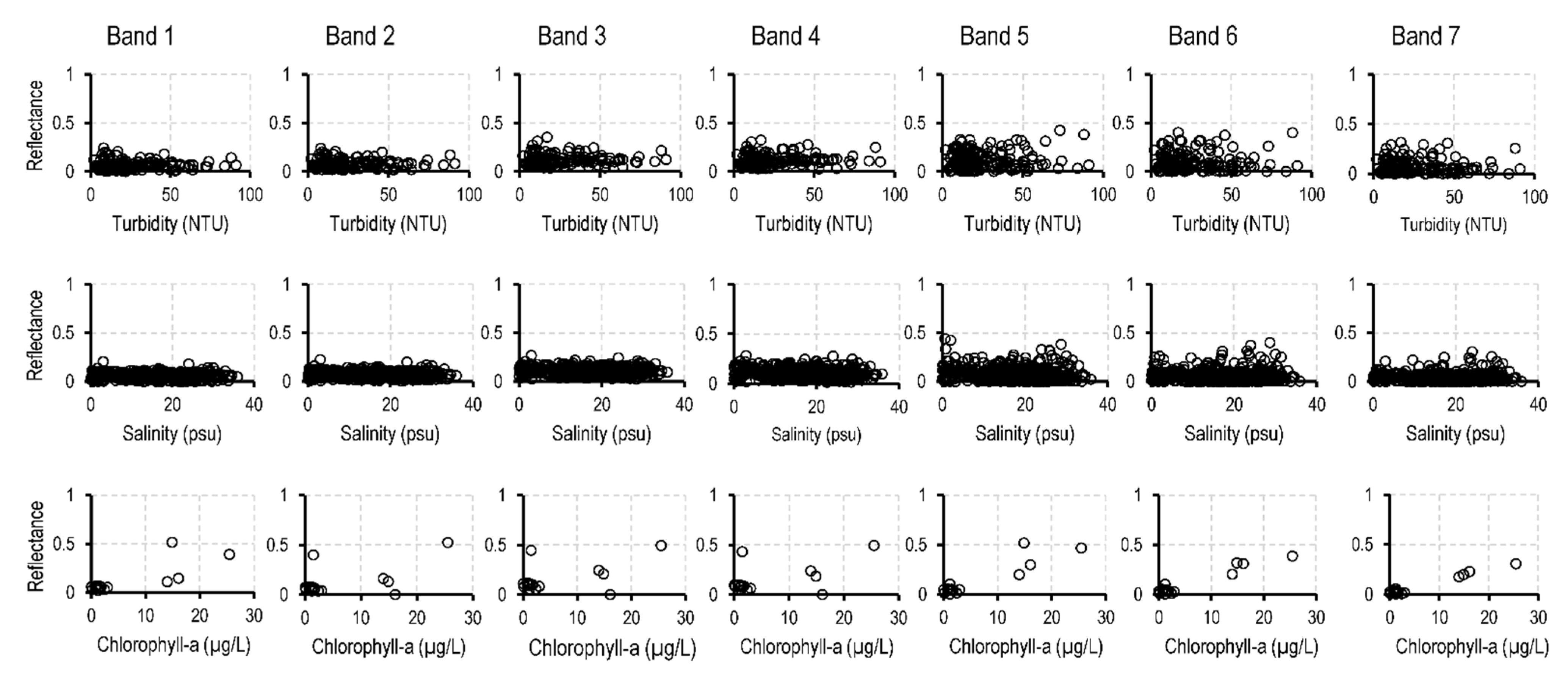
3.1. Surface Reflectance
3.2. Empirical Models
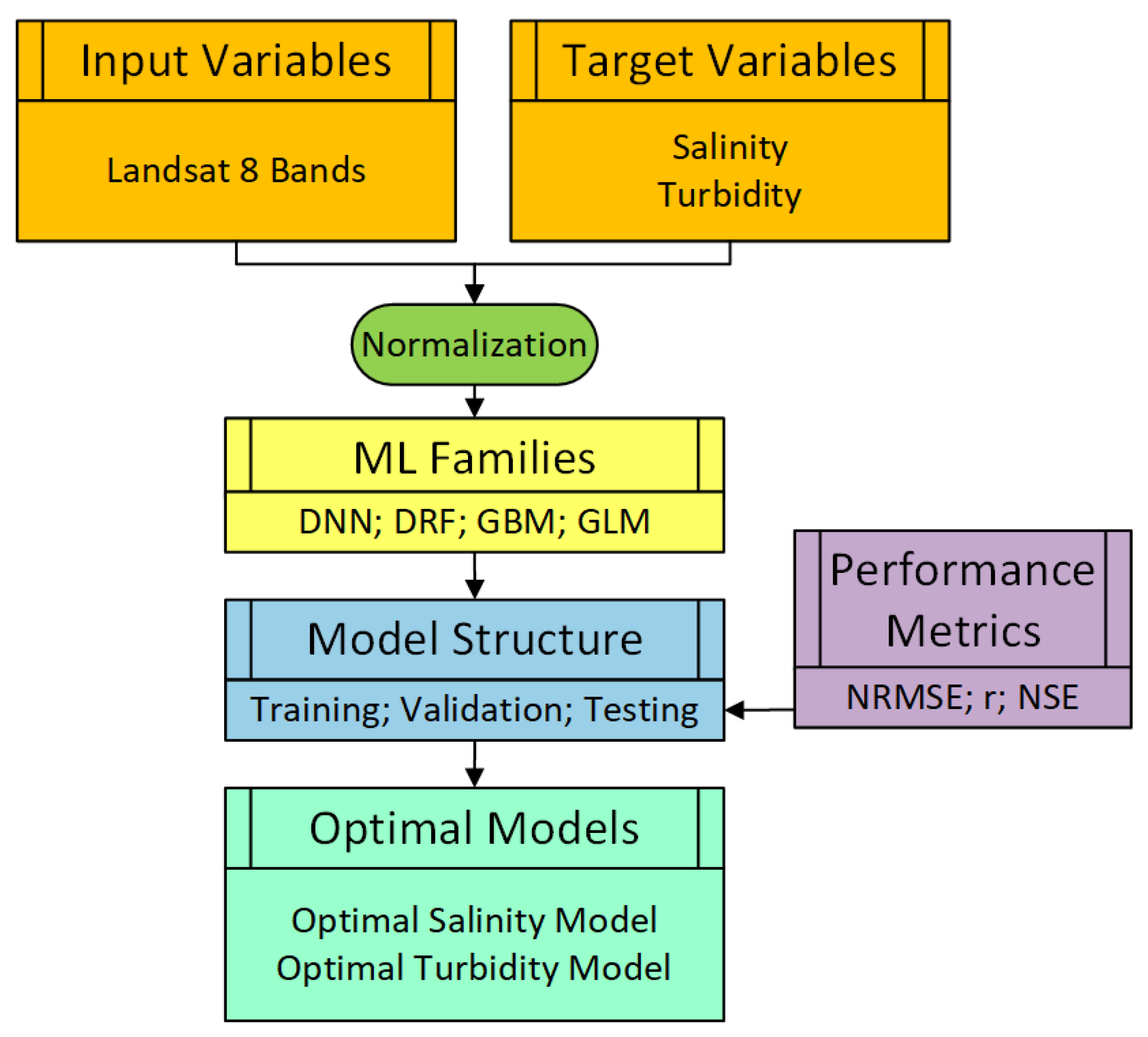
3.3. Machine Learning (ML) Models
3.3.1. ML Model Families
3.3.2. ML Model Setup and Structure
3.4. Model Performance Measures
4. Results
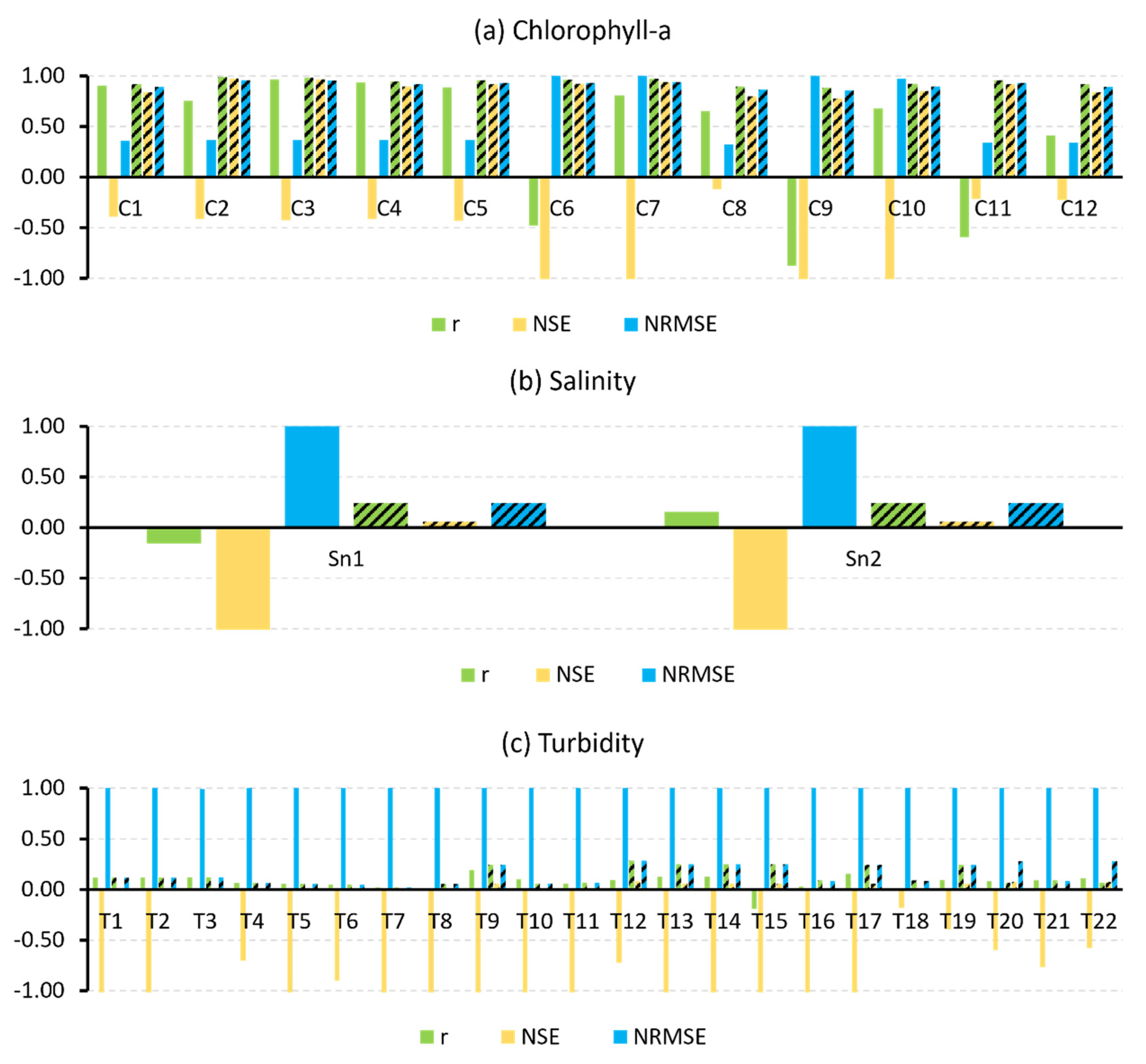
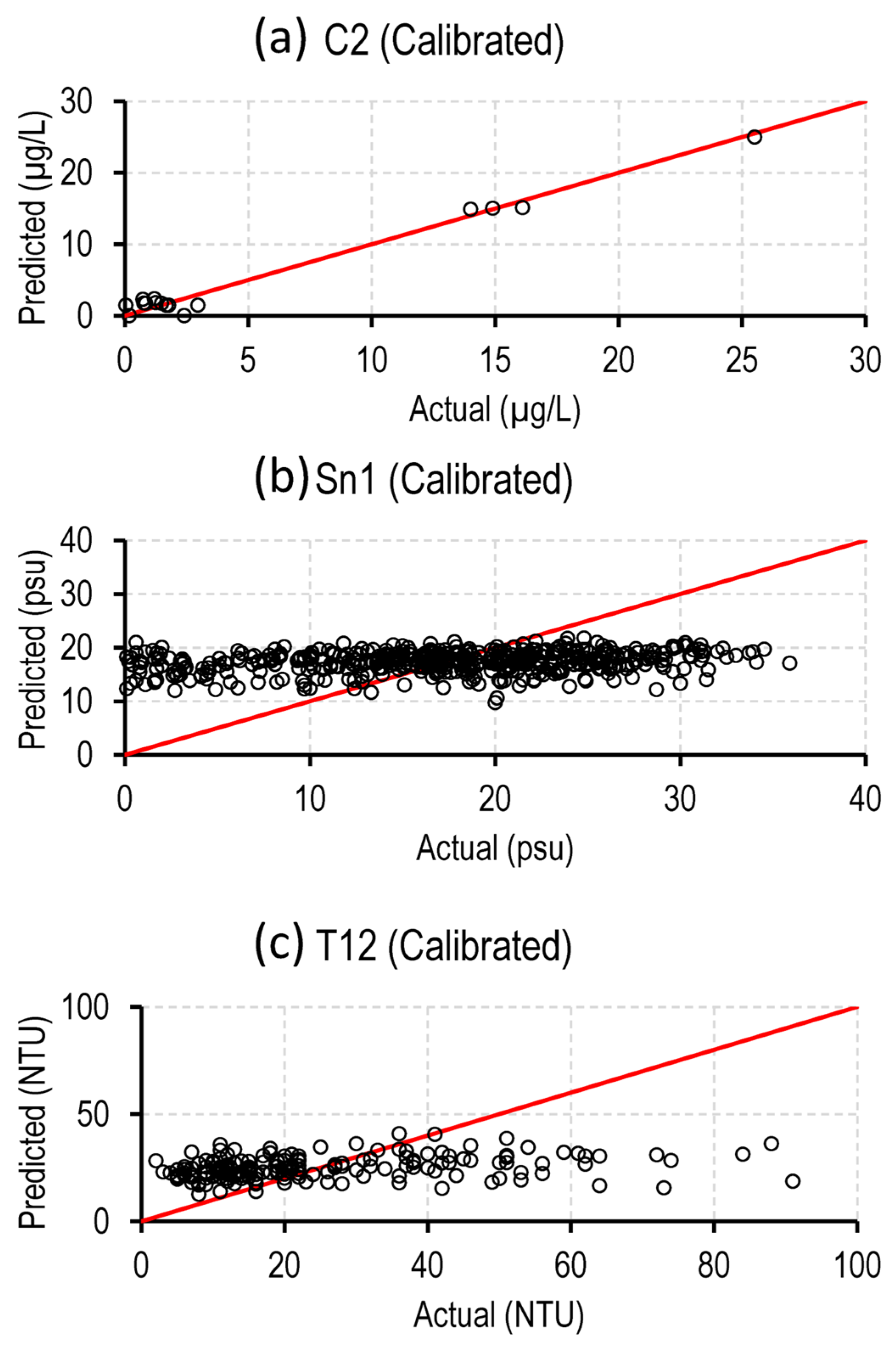
4.1. Empirical Models
4.2. ML Models
4.3. Applications of Optimal Models
5. Discussion
5.1. Empirical Models
5.2. ML Models
6. Conclusions
Author Contributions
Funding
Data Availability Statement
Acknowledgments
Conflicts of Interest
References
- Bugica, K.; Sterba-Boatwright, B.; Wetz, M.S. Water Quality Trends in Texas Estuaries. Mar. Pollut. Bull. 2020, 152, 110903. [Google Scholar] [CrossRef]
- Silva, G.M.; Campos, D.F.; Brasil, J.A.T.; Tremblay, M.; Mendiondo, E.M.; Ghiglieno, F. Advances in Technological Research for Online and In Situ Water Quality Monitoring—A Review. Sustainability 2022, 14, 5059. [Google Scholar] [CrossRef]
- Strobl, R.O.; Robillard, P.D. Network Design for Water Quality Monitoring of Surface Freshwaters: A Review. J. Environ. Manag. 2008, 87, 639–648. [Google Scholar] [CrossRef]
- Wilber, D.H.; Bass, R. Effect of the Colorado River Diversion on Matagorda Bay Epifauna. Estuar. Coast. Shelf Sci. 1998, 47, 309–318. [Google Scholar] [CrossRef]
- Misaghi, F.; Delgosha, F.; Razzaghmanesh, M.; Myers, B. Introducing a Water Quality Index for Assessing Water for Irrigation Purposes: A Case Study of the Ghezel Ozan River. Sci. Total Environ. 2017, 589, 107–116. [Google Scholar] [CrossRef]
- Kumar, A.; Dua, A. Water Quality Index for Assessment of Water Quality of River Ravi at Madhopur (India). Glob. J. Environ. Sci. 2009, 8, 49–57. [Google Scholar] [CrossRef]
- Lim, J.; Choi, M. Assessment of Water Quality Based on Landsat 8 Operational Land Imager Associated with Human Activities in Korea. Environ. Monit. Assess. 2015, 187, 384. [Google Scholar] [CrossRef] [PubMed]
- Kannel, P.R.; Lee, S.; Lee, Y.-S.; Kanel, S.R.; Khan, S.P. Application of Water Quality Indices and Dissolved Oxygen as Indicators for River Water Classification and Urban Impact Assessment. Environ. Monit. Assess. 2007, 132, 93–110. [Google Scholar] [CrossRef]
- Poshtegal, M.K.; Mirbagheri, S.A. Simulation and Modelling of Heavy Metals and Water Quality Parameters in the River. Sci. Rep. 2023, 13, 3020. [Google Scholar] [CrossRef] [PubMed]
- Mishra, A.P.; Khali, H.; Singh, S.; Pande, C.B.; Singh, R.; Chaurasia, S.K. An Assessment of In-Situ Water Quality Parameters and Its Variation with Landsat 8 Level 1 Surface Reflectance Datasets. Int. J. Environ. Anal. Chem. 2021, 103, 1–23. [Google Scholar] [CrossRef]
- Wong, M.-S.; Lee, K.-H.; Kim, Y.-J.; Nichol, J.E.; Li, Z.; Emerson, N. Modeling of Suspended Solids and Sea Surface Salinity in Hong Kong Using Aqua/MODIS Satellite Images. Korean J. Remote Sens. 2007, 23, 161–169. [Google Scholar] [CrossRef]
- AL-Fahdawi, A.A.H.; Rabee, A.M.; Al-Hirmizy, S.M. Water Quality Monitoring of Al-Habbaniyah Lake Using Remote Sensing and in Situ Measurements. Environ. Monit. Assess. 2015, 187, 367. [Google Scholar] [CrossRef] [PubMed]
- Behmel, S.; Damour, M.; Ludwig, R.; Rodriguez, M.J. Water Quality Monitoring Strategies—A Review and Future Perspectives. Sci. Total Environ. 2016, 571, 1312–1329. [Google Scholar] [CrossRef]
- Ighalo, J.O.; Adeniyi, A.G. A Comprehensive Review of Water Quality Monitoring and Assessment in Nigeria. Chemosphere 2020, 260, 127569. [Google Scholar] [CrossRef] [PubMed]
- González-Márquez, L.C.; Torres-Bejarano, F.M.; Torregroza-Espinosa, A.C.; Hansen-Rodríguez, I.R.; Rodríguez-Gallegos, H.B. Use of LANDSAT 8 Images for Depth and Water Quality Assessment of El Guájaro Reservoir, Colombia. J. S. Am. Earth Sci. 2018, 82, 231–238. [Google Scholar] [CrossRef]
- Peterson, K.T.; Sagan, V.; Sloan, J.J. Deep Learning-Based Water Quality Estimation and Anomaly Detection Using Landsat-8/Sentinel-2 Virtual Constellation and Cloud Computing. GIScience Remote Sens. 2020, 57, 510–525. [Google Scholar] [CrossRef]
- Goddijn-Murphy, L.; Dailloux, D.; White, M.; Bowers, D. Fundamentals of in Situ Digital Camera Methodology for Water Quality Monitoring of Coast and Ocean. Sensors 2009, 9, 5825–5843. [Google Scholar] [CrossRef]
- Pahlevan, N.; Smith, B.; Alikas, K.; Anstee, J.; Barbosa, C.; Binding, C.; Bresciani, M.; Cremella, B.; Giardino, C.; Gurlin, D.; et al. Simultaneous Retrieval of Selected Optical Water Quality Indicators from Landsat-8, Sentinel-2, and Sentinel-3. Remote Sens. Environ. 2022, 270, 112860. [Google Scholar] [CrossRef]
- Carpenter, D.J.; Carpenter, S.M. Modeling Inland Water Quality Using Landsat Data. Remote Sens. Environ. 1983, 13, 345–352. [Google Scholar] [CrossRef]
- Sharaf El Din, E. A Novel Approach for Surface Water Quality Modelling Based on Landsat-8 Tasselled Cap Transformation. Int. J. Remote Sens. 2020, 41, 7186–7201. [Google Scholar] [CrossRef]
- Vakili, T.; Amanollahi, J. Determination of Optically Inactive Water Quality Variables Using Landsat 8 Data: A Case Study in Geshlagh Reservoir Affected by Agricultural Land Use. J. Clean. Prod. 2020, 247, 119134. [Google Scholar] [CrossRef]
- Wei, Z.; Wei, L.; Yang, H.; Wang, Z.; Xiao, Z.; Li, Z.; Yang, Y.; Xu, G. Water Quality Grade Identification for Lakes in Middle Reaches of Yangtze River Using Landsat-8 Data with Deep Neural Networks (DNN) Model. Remote Sens. 2022, 14, 6238. [Google Scholar] [CrossRef]
- Markogianni, V.; Kalivas, D.; Petropoulos, G.; Dimitriou, E. Analysis on the Feasibility of Landsat 8 Imagery for Water Quality Parameters Assessment in an Oligotrophic Mediterranean Lake. Int. J. Geol. Environ. Eng. 2017, 11, 906–914. [Google Scholar]
- Sudheer, K.P.; Chaubey, I.; Garg, V. Lake Water Quality Assessment from Landsat Thematic Mapper Data Using Neural Network: An Approach to Optimal Band Combination Selection1. JAWRA J. Am. Water Resour. Assoc. 2006, 42, 1683–1695. [Google Scholar] [CrossRef]
- Zhang, H.; Xue, B.; Wang, G.; Zhang, X.; Zhang, Q. Deep Learning-Based Water Quality Retrieval in an Impounded Lake Using Landsat 8 Imagery: An Application in Dongping Lake. Remote Sens. 2022, 14, 4505. [Google Scholar] [CrossRef]
- González-Márquez, L.C.; Torres-Bejarano, F.M.; Rodríguez-Cuevas, C.; Torregroza-Espinosa, A.C.; Sandoval-Romero, J.A. Estimation of Water Quality Parameters Using Landsat 8 Images: Application to Playa Colorada Bay, Sinaloa, Mexico. Appl. Geomat. 2018, 10, 147–158. [Google Scholar] [CrossRef]
- Ansari, M.; Akhoondzadeh, M. Mapping Water Salinity Using Landsat-8 OLI Satellite Images (Case Study: Karun Basin Located in Iran). Adv. Space Res. 2020, 65, 1490–1502. [Google Scholar] [CrossRef]
- Bayati, M.; Danesh-Yazdi, M. Mapping the Spatiotemporal Variability of Salinity in the Hypersaline Lake Urmia Using Sentinel-2 and Landsat-8 Imagery. J. Hydrol. 2021, 595, 126032. [Google Scholar] [CrossRef]
- Markogianni, V.; Kalivas, D.; Petropoulos, G.P.; Dimitriou, E. An Appraisal of the Potential of Landsat 8 in Estimating Chlorophyll-a, Ammonium Concentrations and Other Water Quality Indicators. Remote Sens. 2018, 10, 1018. [Google Scholar] [CrossRef]
- Hu, C.; Chen, Z.; Clayton, T.D.; Swarzenski, P.; Brock, J.C.; Muller–Karger, F.E. Assessment of Estuarine Water-Quality Indicators Using MODIS Medium-Resolution Bands: Initial Results from Tampa Bay, FL. Remote Sens. Environ. 2004, 93, 423–441. [Google Scholar] [CrossRef]
- Kim, H.-C.; Son, S.; Kim, Y.H.; Khim, J.S.; Nam, J.; Chang, W.K.; Lee, J.-H.; Lee, C.-H.; Ryu, J. Remote Sensing and Water Quality Indicators in the Korean West Coast: Spatio-Temporal Structures of MODIS-Derived Chlorophyll-a and Total Suspended Solids. Mar. Pollut. Bull. 2017, 121, 425–434. [Google Scholar] [CrossRef] [PubMed]
- Huang, W.; Mukherjee, D.; Chen, S. Assessment of Hurricane Ivan Impact on Chlorophyll-a in Pensacola Bay by MODIS 250 m Remote Sensing. Mar. Pollut. Bull. 2011, 62, 490–498. [Google Scholar] [CrossRef] [PubMed]
- Liu, D.; Yu, S.; Cao, Z.; Qi, T.; Duan, H. Process-Oriented Estimation of Column-Integrated Algal Biomass in Eutrophic Lakes by MODIS/Aqua. Int. J. Appl. Earth Obs. Geoinf. 2021, 99, 102321. [Google Scholar] [CrossRef]
- Schaeffer, B.A.; Conmy, R.N.; Duffy, A.E.; Aukamp, J.; Yates, D.F.; Craven, G. Northern Gulf of Mexico Estuarine Coloured Dissolved Organic Matter Derived from MODIS Data. Int. J. Remote Sens. 2015, 36, 2219–2237. [Google Scholar] [CrossRef]
- Yu, X.; Yi, H.; Liu, X.; Wang, Y.; Liu, X.; Zhang, H. Remote-Sensing Estimation of Dissolved Inorganic Nitrogen Concentration in the Bohai Sea Using Band Combinations Derived from MODIS Data. Int. J. Remote Sens. 2016, 37, 327–340. [Google Scholar] [CrossRef]
- Mathew, M.M.; Srinivasa Rao, N.; Mandla, V.R. Development of Regression Equation to Study the Total Nitrogen, Total Phosphorus and Suspended Sediment Using Remote Sensing Data in Gujarat and Maharashtra Coast of India. J. Coast. Conserv. 2017, 21, 917–927. [Google Scholar] [CrossRef]
- Singh, A.; Jakubowski, A.R.; Chidister, I.; Townsend, P.A. A MODIS Approach to Predicting Stream Water Quality in Wisconsin. Remote Sens. Environ. 2013, 128, 74–86. [Google Scholar] [CrossRef]
- Arıman, S. Determination of Inactive Water Quality Variables by MODIS Data: A Case Study in the Kızılırmak Delta-Balik Lake, Turkey. Estuar. Coast. Shelf Sci. 2021, 260, 107505. [Google Scholar] [CrossRef]
- Hossen, H.; Mahmod, W.E.; Negm, A.; Nakamura, T. Assessing Water Quality Parameters in Burullus Lake Using Sentinel-2 Satellite Images. Water Resour. 2022, 49, 321–331. [Google Scholar] [CrossRef]
- Sent, G.; Biguino, B.; Favareto, L.; Cruz, J.; Sá, C.; Dogliotti, A.I.; Palma, C.; Brotas, V.; Brito, A.C. Deriving Water Quality Parameters Using Sentinel-2 Imagery: A Case Study in the Sado Estuary, Portugal. Remote Sens. 2021, 13, 1043. [Google Scholar] [CrossRef]
- Virdis, S.G.P.; Xue, W.; Winijkul, E.; Nitivattananon, V.; Punpukdee, P. Remote Sensing of Tropical Riverine Water Quality Using Sentinel-2 MSI and Field Observations. Ecol. Indic. 2022, 144, 109472. [Google Scholar] [CrossRef]
- Toming, K.; Kutser, T.; Laas, A.; Sepp, M.; Paavel, B.; Nõges, T. First Experiences in Mapping Lake Water Quality Parameters with Sentinel-2 MSI Imagery. Remote Sens. 2016, 8, 640. [Google Scholar] [CrossRef]
- Guo, H.; Huang, J.J.; Chen, B.; Guo, X.; Singh, V.P. A Machine Learning-Based Strategy for Estimating Non-Optically Active Water Quality Parameters Using Sentinel-2 Imagery. Int. J. Remote Sens. 2021, 42, 1841–1866. [Google Scholar] [CrossRef]
- Torres-Bejarano, F.; Arteaga-Hernández, F.; Rodríguez-Ibarra, D.; Mejía-Ávila, D.; González-Márquez, L.C. Water Quality Assessment in a Wetland Complex Using Sentinel 2 Satellite Images. Int. J. Environ. Sci. Technol. 2021, 18, 2345–2356. [Google Scholar] [CrossRef]
- Gorokhovich, Y.; Cawse-Nicholson, K.; Papadopoulos, N.; Oikonomou, D. Use of ECOSTRESS Data for Measurements of the Surface Water Temperature: Significance of Data Filtering in Accuracy Assessment. Remote Sens. Appl. Soc. Environ. 2022, 26, 100739. [Google Scholar] [CrossRef]
- Shi, J.; Hu, C. Evaluation of ECOSTRESS Thermal Data over South Florida Estuaries. Sensors 2021, 21, 4341. [Google Scholar] [CrossRef]
- Ding, H.; Elmore, A.J. Spatio-Temporal Patterns in Water Surface Temperature from Landsat Time Series Data in the Chesapeake Bay, U.S.A. Remote Sens. Environ. 2015, 168, 335–348. [Google Scholar] [CrossRef]
- Shareef, M.A.; Khenchaf, A.; Toumi, A. Integration of Passive and Active Microwave Remote Sensing to Estimate Water Quality Parameters. In Proceedings of the 2016 IEEE Radar Conference (RadarConf), Philadelphia, PA, USA, 2–6 May 2016; pp. 1–4. [Google Scholar]
- Shareef, M.A.; Toumi, A.; Khenchaf, A. Estimation and Characterization of Physical and Inorganic Chemical Indicators of Water Quality by Using SAR Images. In Proceedings of the SAR Image Analysis, Modeling, and Techniques XV, SPIE, Toulouse, France, 15 October 2015; Volume 9642, pp. 140–150. [Google Scholar]
- He, Y.; Jin, S.; Shang, W. Water Quality Variability and Related Factors along the Yangtze River Using Landsat-8. Remote Sens. 2021, 13, 2241. [Google Scholar] [CrossRef]
- Trinh, R.C.; Fichot, C.G.; Gierach, M.M.; Holt, B.; Malakar, N.K.; Hulley, G.; Smith, J. Application of Landsat 8 for Monitoring Impacts of Wastewater Discharge on Coastal Water Quality. Front. Mar. Sci. 2017, 4, 329. [Google Scholar] [CrossRef]
- Wei, L.; Zhang, Y.; Huang, C.; Wang, Z.; Huang, Q.; Yin, F.; Guo, Y.; Cao, L. Inland Lakes Mapping for Monitoring Water Quality Using a Detail/Smoothing-Balanced Conditional Random Field Based on Landsat-8/Levels Data. Sensors 2020, 20, 1345. [Google Scholar] [CrossRef]
- Pu, F.; Ding, C.; Chao, Z.; Yu, Y.; Xu, X. Water-Quality Classification of Inland Lakes Using Landsat8 Images by Convolutional Neural Networks. Remote Sens. 2019, 11, 1674. [Google Scholar] [CrossRef]
- Jakovljević, G.; Govedarica, M.; Álvarez-Taboada, F. Assessment of Biological and Physic Chemical Water Quality Parameters Using Landsat 8 Time Series. In Proceedings of the Remote Sensing for Agriculture, Ecosystems, and Hydrology XX, SPIE, Berlin, Germany, 10 October 2018; Volume 10783, pp. 349–361. [Google Scholar]
- Bormudoi, A.; Hinge, G.; Nagai, M.; Kashyap, M.P.; Talukdar, R. Retrieval of Turbidity and TDS of Deepor Beel Lake from Landsat 8 OLI Data by Regression and Artificial Neural Network. Water Conserv. Sci. Eng. 2022, 7, 505–513. [Google Scholar] [CrossRef]
- Krishnaraj, A.; Honnasiddaiah, R. Remote Sensing and Machine Learning Based Framework for the Assessment of Spatio-Temporal Water Quality in the Middle Ganga Basin. Environ. Sci. Pollut. Res. 2022, 29, 64939–64958. [Google Scholar] [CrossRef] [PubMed]
- Wagle, N.; Acharya, T.D.; Lee, D.H. Comprehensive Review on Application of Machine Learning Algorithms for Water Quality Parameter Estimation Using Remote Sensing Data. Sens. Mater. 2020, 32, 3879. [Google Scholar] [CrossRef]
- Li, N.; Ning, Z.; Chen, M.; Wu, D.; Hao, C.; Zhang, D.; Bai, R.; Liu, H.; Chen, X.; Li, W.; et al. Satellite and Machine Learning Monitoring of Optically Inactive Water Quality Variability in a Tropical River. Remote Sens. 2022, 14, 5466. [Google Scholar] [CrossRef]
- Caillier, J. An Assessment of Benthic Condition in the Matagorda Bay System Using a Sediment Quality Triad Approach. Master’s Thesis, Texas A&M University, Corpus Christi, TX, USA, 2023. [Google Scholar]
- Brody, S.D.; Highfield, W.; Arlikatti, S.; Bierling, D.H.; Ismailova, R.M.; Lee, L.; Butzler, R. Conflict on the Coast: Using Geographic Information Systems to Map Potential Environmental Disputes in Matagorda Bay, Texas. Environ. Manag. 2004, 34, 11–25. [Google Scholar] [CrossRef] [PubMed]
- Aguilar, D.N. Salinity Disturbance Affects Community Structure and Organic Matter on a Restored Crassostrea Virginica Oyster Reef in Matagorda Bay, Texas. Master’s Thesis, Texas A&M University, Corpus Christi, TX, USA, 2017. [Google Scholar]
- Onabule, O.A.; Mitchell, S.B.; Couceiro, F. The Effects of Freshwater Flow and Salinity on Turbidity and Dissolved Oxygen in a Shallow Macrotidal Estuary: A Case Study of Portsmouth Harbour. Ocean Coast. Manag. 2020, 191, 105179. [Google Scholar] [CrossRef]
- Ward, G.H.; Armstrong, N.E. Matagorda Bay, Texas, Its Hydrography, Ecology, and Fishery Resources; Fish and Wildlife Service, U.S. Department of the Interior: Washington, DC, USA, 1980.
- Kinsey, J.; Montagna, P.A. Response of Benthic Organisms to External Conditions in Matagorda Bay; University of Texas, Marine Science Institute: Port Aransas, TX, USA, 2005. [Google Scholar] [CrossRef]
- Marshall, D.A.; Lebreton, B.; Palmer, T.; De Santiago, K.; Beseres Pollack, J. Salinity Disturbance Affects Faunal Community Composition and Organic Matter on a Restored Crassostrea Virginica Oyster Reef. Estuar. Coast. Shelf Sci. 2019, 226, 106267. [Google Scholar] [CrossRef]
- McBride, M.R. Influence of Colorado River Discharge Variability on Phytoplankton Communities in Matagorda Bay, Texas. Master’s Thesis, Texas A&M University, Corpus Christi, TX, USA, 2022. [Google Scholar]
- Armstrong, N. Studies Regarding the Distribution and Biomass Densities of, and the Influences of Freshwater Inflow Variations on Finfish Populations in the Matagorda Bay System, Texas; University of Texas at Austin: Austin, TX, USA, 1987. [Google Scholar]
- Olsen, Z. Quantifying Nursery Habitat Function: Variation in Habitat Suitability Linked to Mortality and Growth for Juvenile Black Drum in a Hypersaline Estuary. Mar. Coast. Fish. 2019, 11, 86–96. [Google Scholar] [CrossRef]
- Renaud, M.; Williams, J. Movements of Kemp’s Ridley (Lepidochelys kempii) and Green (Chelonia mydas) Sea Turtles Using Lavaca Bay and Matagorda Bay; Environmental Protection Agency Office of Planning and Coordination: Dallas, TX, USA, 2023.
- Ropicki, A.; Hanselka, R.; Cummins, D.; Balboa, B.R. The Economic Impacts of Recreational Fishing in the Matagorda Bay System. Available online: https://repository.library.noaa.gov/view/noaa/43595 (accessed on 5 November 2023).
- Haby, M. A Review of Palacios Shrimp Landings, Matagorda Bay Oyster Resources and Statewide Economic Impacts from the Texas Seafood Supply Chain and Saltwater Sportfishing; Sea Grant College Program, Texas A&M University: Corpus Christi, TX, USA, 2016. [Google Scholar]
- Culbertson, J.C. Spatial and Temporal Patterns of Eastern Oyster (Crassostrea virginica) Populations and Their Relationships to Dermo (Perkinsus marinus) Infection and Freshwater Inflows in West Matagorda Bay, Texas. Ph.D. Thesis, Texas A&M University, Corpus Christi, TX, USA, 2008. [Google Scholar]
- Kim, H.-C.; Montagna, P.A. Implications of Colorado River (Texas, USA) Freshwater Inflow to Benthic Ecosystem Dynamics: A Modeling Study. Estuar. Coast. Shelf Sci. 2009, 83, 491–504. [Google Scholar] [CrossRef]
- Grabowski, J.H.; Brumbaugh, R.D.; Conrad, R.F.; Keeler, A.G.; Opaluch, J.J.; Peterson, C.H.; Piehler, M.F.; Powers, S.P.; Smyth, A.R. Economic Valuation of Ecosystem Services Provided by Oyster Reefs. BioScience 2012, 62, 900–909. [Google Scholar] [CrossRef]
- Palmer, T.A.; Montagna, P.A.; Pollack, J.B.; Kalke, R.D.; DeYoe, H.R. The Role of Freshwater Inflow in Lagoons, Rivers, and Bays. Hydrobiologia 2011, 667, 49–67. [Google Scholar] [CrossRef]
- Kucera, C.J.; Faulk, C.K.; Holt, G.J. The Effect of Spawning Salinity on Eggs of Spotted Seatrout (Cynoscion nebulosus, Cuvier) from Two Bays with Historically Different Salinity Regimes. J. Exp. Mar. Biol. Ecol. 2002, 272, 147–158. [Google Scholar] [CrossRef]
- Montagna, P. Inflow Needs Assessment: Effect of the Colorado River Diversion on Benthic Communities; Research Technical Final Report; The University of Texas at Austin: Austin, TX, USA, 1994. [Google Scholar] [CrossRef]
- Armstrong, N. The Ecology of Open-Bay Bottoms of Texas: A Community Profile; U.S. Department of the Interior, Fish and Wildlife Service, Research and Development, National Wetlands Research Center: Washington, DC, USA, 1987.
- TCEQ Surface Water Quality Viewer. Available online: https://tceq.maps.arcgis.com/apps/webappviewer/index.html?id=b0ab6bac411a49189106064b70bbe778 (accessed on 17 August 2023).
- LCRA. Waterquality.Lcra.Org. Available online: https://waterquality.lcra.org/ (accessed on 17 August 2023).
- LCRA. 2022 Guidance for Assessing and Reporting Surface Water Quality in Texas; LCRA: Austin, TX, USA, 2022. [Google Scholar]
- LCRA. Water Quality Parameters—LCRA—Energy, Water, Community; LCRA: Austin, TX, USA, 2023. [Google Scholar]
- TCEQ. Surface Water Quality Monitoring Procedures, Volume 1: Physical and Chemical Monitoring Methods; TCEQ: Austin, TX, USA, 2012.
- Texas Secretary of State Texas Administrative Code. Available online: https://texreg.sos.state.tx.us/public/readtac%24ext.TacPage?sl=T&app=9&p_dir=F&p_rloc=183310&p_tloc=29466&p_ploc=14656&pg=3&p_tac=&ti=30&pt=1&ch=290&rl=111 (accessed on 6 November 2023).
- Dunne, R.P. Spectrophotometric Measurement of Chlorophyll Pigments: A Comparison of Conventional Monochromators and a Reverse Optic Diode Array Design. Mar. Chem. 1999, 66, 245–251. [Google Scholar] [CrossRef]
- Danbara, T.T. Deriving water quality indicators of lake tana, Ethiopia, from Landsat-8. Master’s Thesis, University of Twente, Enschede, The Netherlands, 2014. [Google Scholar]
- Kuhn, C.; de Matos Valerio, A.; Ward, N.; Loken, L.; Sawakuchi, H.O.; Kampel, M.; Richey, J.; Stadler, P.; Crawford, J.; Striegl, R.; et al. Performance of Landsat-8 and Sentinel-2 Surface Reflectance Products for River Remote Sensing Retrievals of Chlorophyll-a and Turbidity. Remote Sens. Environ. 2019, 224, 104–118. [Google Scholar] [CrossRef]
- Mondejar, J.P.; Tongco, A.F. Near Infrared Band of Landsat 8 as Water Index: A Case Study around Cordova and Lapu-Lapu City, Cebu, Philippines. Sustain. Environ. Res. 2019, 29, 16. [Google Scholar] [CrossRef]
- Cabral, P.; Santos, J.A.; Augusto, G. Monitoring Urban Sprawl and the National Ecological Reserve in Sintra-Cascais, Portugal: Multiple OLS Linear Regression Model Evaluation. J. Urban Plan. Dev. 2011, 137, 346–353. [Google Scholar] [CrossRef]
- Peprah, M.S.; Mensah, I.O. Performance Evaluation of the Ordinary Least Square (OLS) and Total Least Square (TLS) in Adjusting Field Data: An Empirical Study on a DGPS Data. S. Afr. J. Geomat. 2017, 6, 73–89. [Google Scholar] [CrossRef]
- Elangovan, A.; Murali, V. Mapping the Chlorophyll-a Concentrations in Hypereutrophic Krishnagiri Reservoir (India) Using Landsat 8 Operational Land Imager. Lakes Reserv. Res. Manag. 2020, 25, 377–387. [Google Scholar] [CrossRef]
- Vargas-Lopez, I.A.; Rivera-Monroy, V.H.; Day, J.W.; Whitbeck, J.; Maiti, K.; Madden, C.J.; Trasviña-Castro, A. Assessing Chlorophyll a Spatiotemporal Patterns Combining In Situ Continuous Fluorometry Measurements and Landsat 8/OLI Data across the Barataria Basin (Louisiana, USA). Water 2021, 13, 512. [Google Scholar] [CrossRef]
- Buditama, G.; Damayanti, A.; Giok Pin, T. Identifying Distribution of Chlorophyll-a Concentration Using Landsat 8 OLI on Marine Waters Area of Cirebon. IOP Conf. Ser. Earth Environ. Sci. 2017, 98, 012040. [Google Scholar] [CrossRef]
- Masocha, M.; Dube, T.; Nhiwatiwa, T.; Choruma, D. Testing Utility of Landsat 8 for Remote Assessment of Water Quality in Two Subtropical African Reservoirs with Contrasting Trophic States. Geocarto Int. 2018, 33, 667–680. [Google Scholar] [CrossRef]
- Yang, Z.; Anderson, Y. Estimating Chlorophyll-A Concentration in a Freshwater Lake Using Landsat 8 Imagery. J. Environ. Earth Sci. 2016, 6, 134–142. [Google Scholar]
- Zhao, J.; Temimi, M. An Empirical Algorithm for Retreiving Salinity in the Arabian Gulf: Application to Landsat-8 Data. In Proceedings of the 2016 IEEE International Geoscience and Remote Sensing Symposium (IGARSS), Beijing, China, 10–15 July 2016; pp. 4645–4648. [Google Scholar]
- Zhao, J.; Temimi, M.; Ghedira, H. Remotely Sensed Sea Surface Salinity in the Hyper-Saline Arabian Gulf: Application to Landsat 8 OLI Data. Estuar. Coast. Shelf Sci. 2017, 187, 168–177. [Google Scholar] [CrossRef]
- Snyder, J.; Boss, E.; Weatherbee, R.; Thomas, A.C.; Brady, D.; Newell, C. Oyster Aquaculture Site Selection Using Landsat 8-Derived Sea Surface Temperature, Turbidity, and Chlorophyll a. Front. Mar. Sci. 2017, 4, 190. [Google Scholar] [CrossRef]
- Quang, N.H.; Sasaki, J.; Higa, H.; Huan, N.H. Spatiotemporal Variation of Turbidity Based on Landsat 8 OLI in Cam Ranh Bay and Thuy Trieu Lagoon, Vietnam. Water 2017, 9, 570. [Google Scholar] [CrossRef]
- Liu, L.-W.; Wang, Y.-M. Modelling Reservoir Turbidity Using Landsat 8 Satellite Imagery by Gene Expression Programming. Water 2019, 11, 1479. [Google Scholar] [CrossRef]
- Allam, M.; Yawar Ali Khan, M.; Meng, Q. Retrieval of Turbidity on a Spatio-Temporal Scale Using Landsat 8 SR: A Case Study of the Ramganga River in the Ganges Basin, India. Appl. Sci. 2020, 10, 3702. [Google Scholar] [CrossRef]
- Pereira, L.S.F.; Andes, L.C.; Cox, A.L.; Ghulam, A. Measuring Suspended-Sediment Concentration and Turbidity in the Middle Mississippi and Lower Missouri Rivers Using Landsat Data. JAWRA J. Am. Water Resour. Assoc. 2018, 54, 440–450. [Google Scholar] [CrossRef]
- Truong, A.; Walters, A.; Goodsitt, J.; Hines, K.; Bruss, C.B.; Farivar, R. Towards Automated Machine Learning: Evaluation and Comparison of AutoML Approaches and Tools. In Proceedings of the 2019 IEEE 31st International Conference on Tools with Artificial Intelligence (ICTAI), Portland, OR, USA, 4–6 November 2019; pp. 1471–1479. [Google Scholar]
- Kamilaris, A.; Prenafeta-Boldú, F.X. Deep Learning in Agriculture: A Survey. Comput. Electron. Agric. 2018, 147, 70–90. [Google Scholar] [CrossRef]
- Mathew, A.; Amudha, P.; Sivakumari, S. Deep Learning Techniques: An Overview. In Proceedings of the Advanced Machine Learning Technologies and Applications, Jaipur, India, 13–15 February 2020; Hassanien, A.E., Bhatnagar, R., Darwish, A., Eds.; Springer: Singapore, 2021; pp. 599–608. [Google Scholar]
- Oyebisi, S.; Alomayri, T. Artificial Intelligence-Based Prediction of Strengths of Slag-Ash-Based Geopolymer Concrete Using Deep Neural Networks. Constr. Build. Mater. 2023, 400, 132606. [Google Scholar] [CrossRef]
- Tang, C.; Luktarhan, N.; Zhao, Y. SAAE-DNN: Deep Learning Method on Intrusion Detection. Symmetry 2020, 12, 1695. [Google Scholar] [CrossRef]
- Asgari, M.; Yang, W.; Farnaghi, M. Spatiotemporal Data Partitioning for Distributed Random Forest Algorithm: Air Quality Prediction Using Imbalanced Big Spatiotemporal Data on Spark Distributed Framework. Environ. Technol. Innov. 2022, 27, 102776. [Google Scholar] [CrossRef]
- Shrivastav, L.K.; Kumar, R. An Ensemble of Random Forest Gradient Boosting Machine and Deep Learning Methods for Stock Price Prediction. J. Inf. Technol. Res. (JITR) 2022, 15, 1–19. [Google Scholar] [CrossRef]
- Natekin, A.; Knoll, A. Gradient Boosting Machines, a Tutorial. Front. Neurorobot. 2013, 7, 21. [Google Scholar] [CrossRef] [PubMed]
- Pekár, S.; Brabec, M. Generalized Estimating Equations: A Pragmatic and Flexible Approach to the Marginal GLM Modelling of Correlated Data in the Behavioural Sciences. Ethology 2018, 124, 86–93. [Google Scholar] [CrossRef]
- Osawa, T.; Mitsuhashi, H.; Uematsu, Y.; Ushimaru, A. Bagging GLM: Improved Generalized Linear Model for the Analysis of Zero-Inflated Data. Ecol. Inform. 2011, 6, 270–275. [Google Scholar] [CrossRef]
- Masocha, M.; Mungenge, C.; Nhiwatiwa, T. Remote Sensing of Nutrients in a Subtropical African Reservoir: Testing Utility of Landsat 8. Geocarto Int. 2018, 33, 458–469. [Google Scholar] [CrossRef]
- Davies-Colley, R.J.; Smith, D.G. Turbidity Suspeni)Ed Sediment, and Water Clarity: A Review1. JAWRA J. Am. Water Resour. Assoc. 2001, 37, 1085–1101. [Google Scholar] [CrossRef]
- Boyer, J.N.; Kelble, C.R.; Ortner, P.B.; Rudnick, D.T. Phytoplankton Bloom Status: Chlorophyll a Biomass as an Indicator of Water Quality Condition in the Southern Estuaries of Florida, USA. Ecol. Indic. 2009, 9, S56–S67. [Google Scholar] [CrossRef]
- Kasprzak, P.; Padisák, J.; Koschel, R.; Krienitz, L.; Gervais, F. Chlorophyll a Concentration across a Trophic Gradient of Lakes: An Estimator of Phytoplankton Biomass? Limnologica 2008, 38, 327–338. [Google Scholar] [CrossRef]
- Rakocevic-Nedovic, J.; Hollert, H. Phytoplankton Community and Chlorophyll a as Trophic State Indices of Lake Skadar (Montenegro, Balkan) (7 Pp). Environ. Sci. Poll. Res. Int. 2005, 12, 146–152. [Google Scholar] [CrossRef]
- El-Zeiny, A.; El-Kafrawy, S. Assessment of Water Pollution Induced by Human Activities in Burullus Lake Using Landsat 8 Operational Land Imager and GIS. Egypt. J. Remote Sens. Space Sci. 2017, 20, S49–S56. [Google Scholar] [CrossRef]
- Schild, K.M.; Hawley, R.L.; Chipman, J.W.; Benn, D.I. Quantifying Suspended Sediment Concentration in Subglacial Sediment Plumes Discharging from Two Svalbard Tidewater Glaciers Using Landsat-8 and in Situ Measurements. Int. J. Remote Sens. 2017, 38, 6865–6881. [Google Scholar] [CrossRef]
- Kaufman, Y.J.; Tanré, D.; Gordon, H.R.; Nakajima, T.; Lenoble, J.; Frouin, R.; Grassl, H.; Herman, B.M.; King, M.D.; Teillet, P.M. Passive Remote Sensing of Tropospheric Aerosol and Atmospheric Correction for the Aerosol Effect. J. Geophys. Res. Atmos. 1997, 102, 16815–16830. [Google Scholar] [CrossRef]
- Vermote, E.; Justice, C.; Claverie, M.; Franch, B. Preliminary Analysis of the Performance of the Landsat 8/OLI Land Surface Reflectance Product. Remote Sens. Environ. 2016, 185, 46–56. [Google Scholar] [CrossRef]
- Misra, A.; Chapron, B.; Nouguier, F.; Ramakrishnan, B.; Yurovskaya, M. Sun-Glint Imagery of Landsat 8 for Ocean Surface Waves. In Proceedings of the Remote Sensing of the Open and Coastal Ocean and Inland Waters, SPIE, Honolulu, HI, USA, 24 October 2018; Volume 10778, pp. 86–94. [Google Scholar]
- Wei, J.; Lee, Z.; Garcia, R.; Zoffoli, L.; Armstrong, R.A.; Shang, Z.; Sheldon, P.; Chen, R.F. An Assessment of Landsat-8 Atmospheric Correction Schemes and Remote Sensing Reflectance Products in Coral Reefs and Coastal Turbid Waters. Remote Sens. Environ. 2018, 215, 18–32. [Google Scholar] [CrossRef]
- Pahlevan, N.; Schott, J.R.; Franz, B.A.; Zibordi, G.; Markham, B.; Bailey, S.; Schaaf, C.B.; Ondrusek, M.; Greb, S.; Strait, C.M. Landsat 8 Remote Sensing Reflectance (Rrs) Products: Evaluations, Intercomparisons, and Enhancements. Remote Sens. Environ. 2017, 190, 289–301. [Google Scholar] [CrossRef]
- Wang, F.; Xu, Y.J. Development and Application of a Remote Sensing-Based Salinity Prediction Model for a Large Estuarine Lake in the US Gulf of Mexico Coast. J. Hydrol. 2008, 360, 184–194. [Google Scholar] [CrossRef]
- Binding, C.E.; Bowers, D.G. Measuring the Salinity of the Clyde Sea from Remotely Sensed Ocean Colour. Estuar. Coast. Shelf Sci. 2003, 57, 605–611. [Google Scholar] [CrossRef]
- Bowers, D.G.; Brett, H.L. The Relationship between CDOM and Salinity in Estuaries: An Analytical and Graphical Solution. J. Mar. Syst. 2008, 73, 1–7. [Google Scholar] [CrossRef]
- Fang, L.; Chen, S.; Wang, H.; Qian, J.; Zhang, L. Detecting Marine Intrusion into Rivers Using EO-1 ALI Satellite Imagery: Modaomen Waterway, Pearl River Estuary, China. Int. J. Remote Sens. 2010, 31, 4125–4146. [Google Scholar] [CrossRef]
- Lavery, P.; Pattiaratchi, C.; Wyllie, A.; Hick, P. Water Quality Monitoring in Estuarine Waters Using the Landsat Thematic Mapper. Remote Sens. Environ. 1993, 46, 268–280. [Google Scholar] [CrossRef]
- Vuille, M.; Baumgartner, M.F. Hydrologic Investigations in the North Chilean Altiplano Using Landsat-MSS and -TM Data. Geocarto Int. 1993, 8, 35–45. [Google Scholar] [CrossRef]
- Zhang, C.; Xie, Z.; Roberts, C.; Berry, L.; Chen, G. Salinity Assessment in Northeast Florida Bay Using Landsat TM Data. Southeast. Geogr. 2012, 52, 267–281. [Google Scholar] [CrossRef]
- Xie, Z.; Zhang, C.; Berry, L. Geographically Weighted Modelling of Surface Salinity in Florida Bay Using Landsat TM Data. Remote Sens. Lett. 2013, 4, 75–83. [Google Scholar] [CrossRef]
- Khorram, S. Development of Water Quality Models Applicable throughout the Entire San Francisco Bay and Delta. Photogramm. Eng. Remote Sens. 1985, 51, 53–62. [Google Scholar]
- Nazeer, M.; Bilal, M. Evaluation of Ordinary Least Square (OLS) and Geographically Weighted Regression (GWR) for Water Quality Monitoring: A Case Study for the Estimation of Salinity. J. Ocean Univ. China 2018, 17, 305–310. [Google Scholar] [CrossRef]
- Urquhart, E.; Zaitchik, B.; Hoffman, M.; Guikema, S.; Geiger, E. Remotely Sensed Estimates of Surface Salinity in the Chesapeake Bay: A Statistical Approach. Remote Sens. Environ. 2012, 123, 522–531. [Google Scholar] [CrossRef]
- Nguyen, P.; Koedsin, W.; McNeil, D.; Van, T. Remote Sensing Techniques to Predict Salinity Intrusion: Application for a Data-Poor Area of the Coastal Mekong Delta, Vietnam. Int. J. Remote Sens. 2018, 39, 6676. [Google Scholar] [CrossRef]
- Zhu, M.; Wang, J.; Yang, X.; Zhang, Y.; Zhang, L.; Ren, H.; Wu, B.; Ye, L. A Review of the Application of Machine Learning in Water Quality Evaluation. Eco-Environ. Health 2022, 1, 107–116. [Google Scholar] [CrossRef] [PubMed]
- Guo, H.; Tian, S.; Jeanne Huang, J.; Zhu, X.; Wang, B.; Zhang, Z. Performance of Deep Learning in Mapping Water Quality of Lake Simcoe with Long-Term Landsat Archive. ISPRS J. Photogramm. Remote Sens. 2022, 183, 451–469. [Google Scholar] [CrossRef]
- Sun, A.; Scanlon, B.; Save, H.; Rateb, A. Reconstruction of GRACE Total Water Storage Through Automated Machine Learning. Water Resour. Res. 2021, 57, e2020WR028666. [Google Scholar] [CrossRef]
- Fallatah, O.; Ahmed, M.; Gyawali, B.; Alhawsawi, A. Factors Controlling Groundwater Radioactivity in Arid Environments: An Automated Machine Learning Approach. Sci. Total Environ. 2022, 830, 154707. [Google Scholar] [CrossRef]


| WQI | Units | No. of Samples | Max. Value | Min. Value | Mean Value | St. Dev. 2 |
|---|---|---|---|---|---|---|
| Salinity | psu | 478 | 35.91 | 0.10 | 17.37 | 8.22 |
| Turbidity | NTU | 173 | 91.00 | 2.00 | 25.18 | 18.60 |
| Chlorophyll-a | µg/L | 17 | 25.50 | 0.04 | 5.11 | 7.55 |
| WQI | Salinity (478) | Turbidity (173) | Chlorophyll-a (17) | |
|---|---|---|---|---|
| B1 | Min. | 0.00 | 0.00 | 0.02 |
| Max. | 0.20 | 0.24 | 0.52 | |
| Mean | 0.05 | 0.06 | 0.10 | |
| St. Dev. 2 | 0.03 | 0.04 | 0.14 | |
| B2 | Min. | 0.01 | 0.01 | 0.04 |
| Max. | 0.23 | 0.24 | 0.52 | |
| Mean | 0.07 | 0.08 | 0.12 | |
| St. Dev. | 0.03 | 0.04 | 0.13 | |
| B3 | Min. | 0.02 | 0.04 | 0.06 |
| Max. | 0.27 | 0.35 | 0.49 | |
| Mean | 0.11 | 0.12 | 0.15 | |
| St. Dev. | 0.04 | 0.05 | 0.13 | |
| B4 | Min. | 0.01 | 0.03 | 0.04 |
| Max. | 0.28 | 0.32 | 0.49 | |
| Mean | 0.11 | 0.11 | 0.14 | |
| St. Dev. | 0.05 | 0.06 | 0.13 | |
| B5 | Min. | 0.00 | 0.00 | 0.00 |
| Max. | 0.44 | 0.42 | 0.52 | |
| Mean | 0.08 | 0.12 | 0.12 | |
| St. Dev. | 0.07 | 0.09 | 0.16 | |
| B6 | Min. | 0.00 | 0.00 | 0.00 |
| Max. | 0.40 | 0.40 | 0.39 | |
| Mean | 0.06 | 0.10 | 0.10 | |
| St. Dev. | 0.06 | 0.09 | 0.12 | |
| B7 | Min. | 0.00 | 0.00 | 0.00 |
| Max. | 0.31 | 0.32 | 0.31 | |
| Mean | 0.04 | 0.07 | 0.07 | |
| St. Dev. | 0.04 | 0.07 | 0.09 | |
| WQI | Model ID | Equation | Location | Source |
|---|---|---|---|---|
| Chlorophyll-a | C1 | Krishnagiri Reservoir, India | [91] | |
| Matagorda Bay | — | |||
| C2 | Krishnagiri Reservoir, India | [91] | ||
| Matagorda Bay | — | |||
| C3 | Krishnagiri Reservoir, India | [91] | ||
| Matagorda Bay | — | |||
| C4 | Krishnagiri Reservoir, India | [91] | ||
| Matagorda Bay | — | |||
| C5 | Krishnagiri Reservoir, India | [91] | ||
| Matagorda Bay | — | |||
| C6 | Barataria Basin, Mississippi | [92] | ||
| Matagorda Bay | — | |||
| C7 | Trichonis Lake, Greece | [29] | ||
| Matagorda Bay | — | |||
| C8 | Java Sea, Cirebon | [93] | ||
| Matagorda Bay | — | |||
| C9 | Lake Chivero, Zimbabwe | [94] | ||
| Matagorda Bay | — | |||
| C10 | Lake Chivero, Zimbabwe | [94] | ||
| Matagorda Bay | — | |||
| C11 | Jordan Lake, North Carolina | [95] | ||
| Matagorda Bay | — | |||
| C12 | Jordan Lake, North Carolina | [95] | ||
| Matagorda Bay | — | |||
| Salinity | Sn1 | Arabian Gulf | [96] | |
| Matagorda Bay | — | |||
| Sn2 | Arabian Gulf | [97] | ||
| Matagorda Bay | — | |||
| Turbidity | T1 | Damariscotta River and Harpswell Sound Bay, Maine | [98] | |
| Matagorda Bay | ||||
| T2 | Cam Ranh Bay (CRB) and Thuy Trieu Lagoon (TTL), Vietnam | [99] | ||
| Matagorda Bay | — | |||
| T3 | CRB and TTL, Vietnam | [99] | ||
| Matagorda Bay | — | |||
| T4 | CRB and TTL, Vietnam | [99] | ||
| Matagorda Bay | — | |||
| T5 | CRB and TTL, Vietnam | [99] | ||
| Matagorda Bay | — | |||
| T6 | CRB and TTL, Vietnam | [99] | ||
| Matagorda Bay | — | |||
| T7 | CRB and TTL, Vietnam | [99] | ||
| Matagorda Bay | — | |||
| T8 | CRB and TTL, Vietnam | [99] | ||
| Matagorda Bay | — | |||
| T9 | CRB and TTL, Vietnam | [99] | ||
| Matagorda Bay | — | |||
| T10 | CRB and TTL, Vietnam | [99] | ||
| Matagorda Bay | — | |||
| T11 | CRB and TTL, Vietnam | [99] | ||
| Matagorda Bay | — | |||
| T12 | 4.21 − 74.26(B2) − 14.84(B3) + 267.24(B4) − 126.89(B5) | Tsegn-Wen and Nan-Haw Reservoir, Taiwan | [100] | |
| Matagorda Bay | — | |||
| T13 | Lake Chivero, Zimbabwe | [94] | ||
| Matagorda Bay | ||||
| T14 | Lake Chivero, Zimbabwe | [94] | ||
| Matagorda Bay | — | |||
| T15 | Ramganga River, India | [101] | ||
| Matagorda Bay | ||||
| T16 | Ramganga River, India | [101] | ||
| Matagorda Bay | — | |||
| T17 | Mississippi River, Mississippi | [102] | ||
| Matagorda Bay | — | |||
| T18 | Tseng-Wen reservoir, Taiwan | [100] | ||
| Matagorda Bay | — | |||
| T19 | Tseng-Wen reservoir, Taiwan | [100] | ||
| Matagorda Bay | — | |||
| T20 | Tseng-Wen reservoir, Taiwan | [100] | ||
| Matagorda Bay | — | |||
| T21 | Tseng-Wen reservoir, Taiwan | [100] | ||
| Matagorda Bay | — | |||
| T22 | Tseng-Wen reservoir, Taiwan | [100] | ||
| Matagorda Bay | — |
| WQI | Model ID | Uncalibrated Models | Calibrated Models | ||||
|---|---|---|---|---|---|---|---|
| NRMSE | r | NSE | NRMSE | r | NSE | ||
| Chlorophyll-a | C1 | 0.36 | 0.90 | −0.39 | 0.89 | 0.92 | 0.84 |
| C2 | 0.36 | 0.75 | −0.41 | 0.96 | 0.99 | 0.98 | |
| C3 | 0.36 | 0.96 | −0.43 | 0.95 | 0.98 | 0.96 | |
| C4 | 0.36 | 0.93 | −0.42 | 0.92 | 0.94 | 0.89 | |
| C5 | 0.36 | 0.89 | −0.43 | 0.93 | 0.96 | 0.92 | |
| C6 | 7.00 | −0.48 | −528.50 | 0.93 | 0.96 | 0.92 | |
| C7 | 1475.10 | 0.80 | −23,527,276.57 | 0.94 | 0.97 | 0.94 | |
| C8 | 0.32 | 0.65 | −0.12 | 0.87 | 0.89 | 0.80 | |
| C9 | 37.08 | −0.88 | −14,866.34 | 0.85 | 0.88 | 0.77 | |
| C10 | 0.97 | 0.68 | −9.18 | 0.89 | 0.92 | 0.85 | |
| C11 | 0.34 | −0.60 | −0.22 | 0.93 | 0.96 | 0.92 | |
| C12 | 0.34 | 0.41 | −0.23 | 0.89 | 0.92 | 0.84 | |
| Salinity | Sn1 | 180.48 | −0.16 | −32,638.62 | 0.24 | 0.24 | 0.06 |
| Sn2 | 180.47 | 0.16 | −32,635.55 | 0.24 | 0.24 | 0.06 | |
| Turbidity | T1 | 5.18 | 0.12 | −26.00 | 0.12 | 0.12 | 0.01 |
| T2 | 1.65 | 0.12 | −1.75 | 0.12 | 0.12 | 0.01 | |
| T3 | 0.99 | 0.12 | 0.01 | 0.12 | 0.12 | 0.01 | |
| T4 | 1.30 | 0.07 | −0.70 | 0.07 | 0.07 | 0.00 | |
| T5 | 3.85 | 0.06 | −13.90 | 0.06 | 0.06 | 0.00 | |
| T6 | 1.37 | 0.05 | −0.90 | 0.05 | 0.05 | 0.00 | |
| T7 | 1.50 | 0.02 | −1.25 | 0.02 | 0.02 | 0.00 | |
| T8 | 4.12 | 0.01 | −16.05 | 0.06 | 0.06 | 0.00 | |
| T9 | 1.53 | 0.19 | −1.34 | 0.25 | 0.25 | 0.06 | |
| T10 | 1.41 | 0.10 | −1.01 | 0.06 | 0.06 | 0.00 | |
| T11 | 1.41 | 0.06 | −1.01 | 0.07 | 0.07 | 0.00 | |
| T12 | 1.31 | 0.09 | −0.72 | 0.29 | 0.29 | 0.08 | |
| T13 | 85.15 | 0.13 | −7292.28 | 0.25 | 0.25 | 0.06 | |
| T14 | 7.22 | 0.13 | −51.39 | 0.25 | 0.25 | 0.06 | |
| T15 | 1.56 | −0.19 | −1.45 | 0.25 | 0.25 | 0.06 | |
| T16 | 1.63 | 0.03 | −1.68 | 0.09 | 0.09 | 0.01 | |
| T17 | 1.74 | 0.16 | −2.06 | 0.25 | 0.25 | 0.06 | |
| T18 | 1.09 | −0.01 | −0.18 | 0.09 | 0.09 | 0.01 | |
| T19 | 1.18 | 0.09 | −0.39 | 0.25 | 0.25 | 0.06 | |
| T20 | 1.26 | 0.08 | −0.60 | 0.28 | 0.07 | 0.08 | |
| T21 | 1.32 | 0.09 | −0.77 | 0.09 | 0.09 | 0.01 | |
| T22 | 1.25 | 0.11 | −0.58 | 0.28 | 0.07 | 0.08 | |
| WQI | ML Family | Training | Testing | ||||
|---|---|---|---|---|---|---|---|
| NRMSE | r | NSE | NRMSE | r | NSE | ||
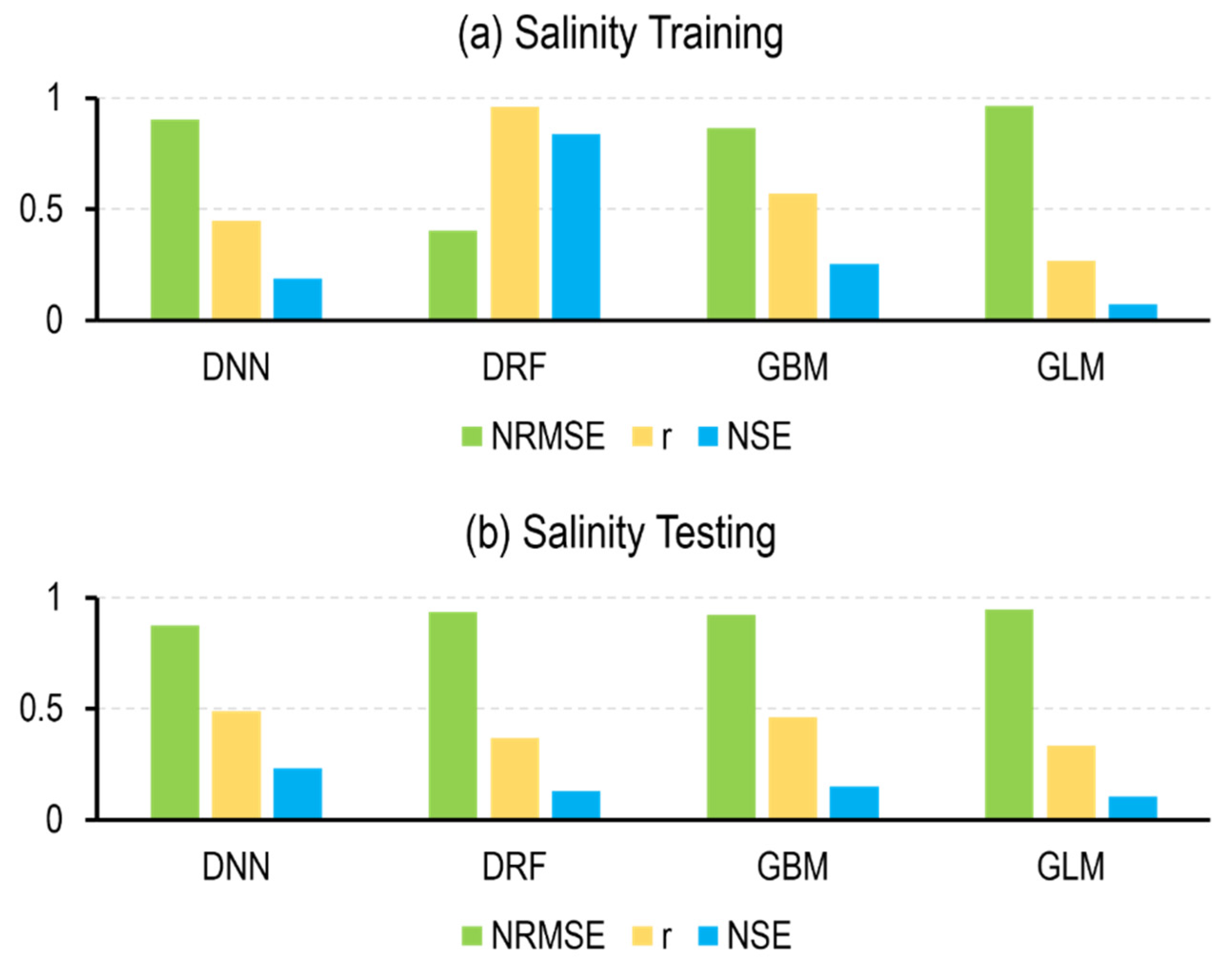
| Salinity | DNN | 0.90 ± 0.08 | 0.45 ± 0.10 | 0.19 ± 0.13 | 0.87 ± 0.06 | 0.49 ± 0.09 | 0.23 ± 0.12 |
| DRF | 0.40 ± 0.01 | 0.96 ± 0.00 | 0.84 ± 0.01 | 0.93 ± 0.04 | 0.37 ± 0.08 | 0.13 ± 0.08 | |
| GBM | 0.86 ± 0.04 | 0.57 ± 0.07 | 0.25 ± 0.07 | 0.92 ± 0.03 | 0.46 ± 0.10 | 0.15 ± 0.07 | |
| GLM | 0.96 ± 0.01 | 0.27 ± 0.02 | 0.07 ± 0.01 | 0.95 ± 0.03 | 0.33 ± 0.08 | 0.10 ± 0.05 | |
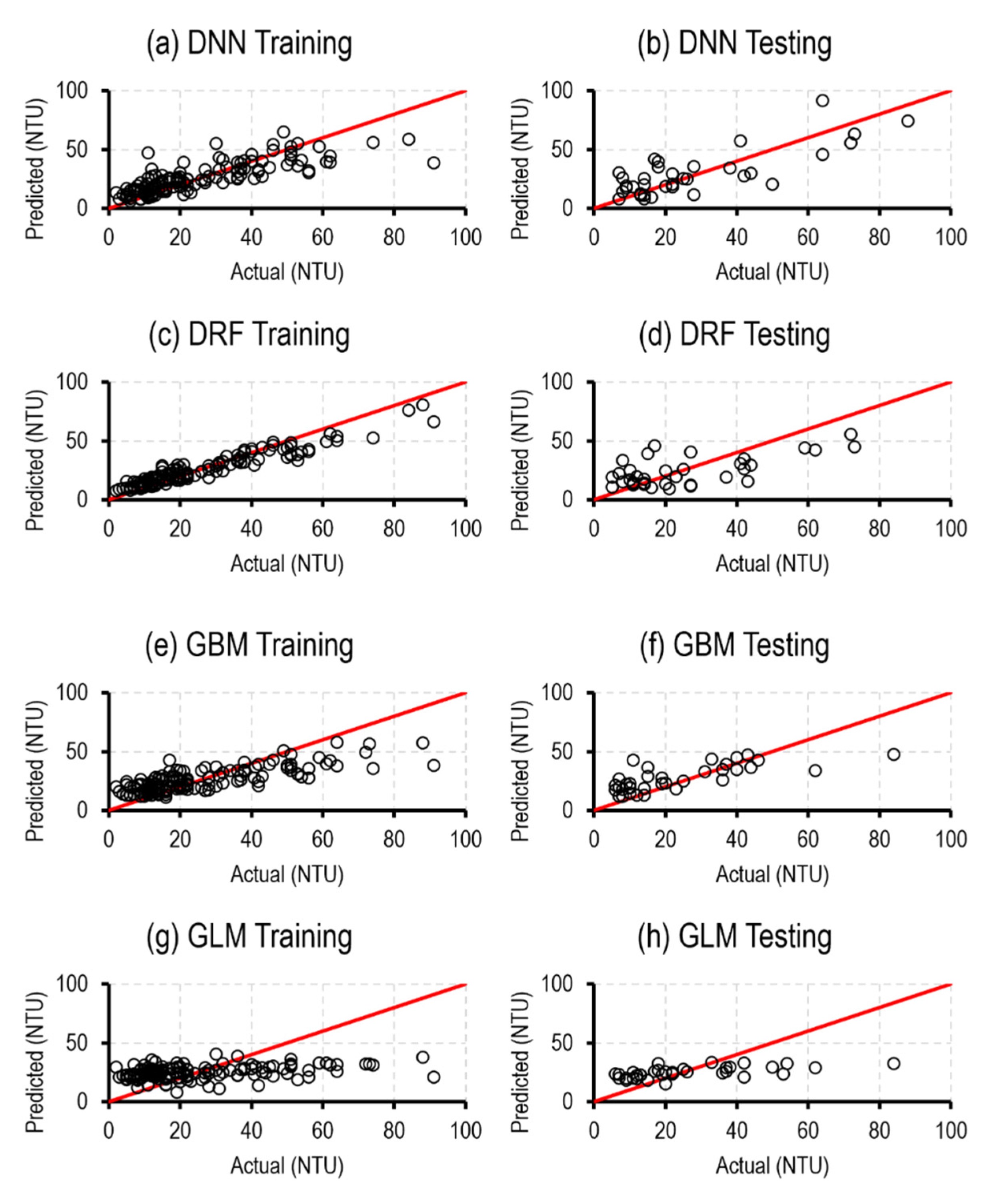
| Turbidity | DNN | 0.59 ± 0.13 | 0.81 ± 0.06 | 0.65 ± 0.11 | 0.63 ± 0.11 | 0.79 ± 0.11 | 0.60 ± 0.20 |
| DRF | 0.36 ± 0.02 | 0.95 ± 0.01 | 0.87 ± 0.01 | 0.76 ± 0.10 | 0.65 ± 0.11 | 0.42 ± 0.18 | |
| GBM | 0.66 ± 0.17 | 0.79 ± 0.07 | 0.56 ± 0.14 | 0.73 ± 0.10 | 0.73 ± 0.13 | 0.47 ± 0.20 | |
| GLM | 0.93 ± 0.03 | 0.36 ± 0.08 | 0.13 ± 0.05 | 0.86 ± 0.07 | 0.63 ± 0.16 | 0.25 ± 0.14 | |
Disclaimer/Publisher’s Note: The statements, opinions and data contained in all publications are solely those of the individual author(s) and contributor(s) and not of MDPI and/or the editor(s). MDPI and/or the editor(s) disclaim responsibility for any injury to people or property resulting from any ideas, methods, instructions or products referred to in the content. |
© 2024 by the authors. Licensee MDPI, Basel, Switzerland. This article is an open access article distributed under the terms and conditions of the Creative Commons Attribution (CC BY) license (https://creativecommons.org/licenses/by/4.0/).
Share and Cite
Bygate, M.; Ahmed, M. Monitoring Water Quality Indicators over Matagorda Bay, Texas, Using Landsat-8. Remote Sens. 2024, 16, 1120. https://doi.org/10.3390/rs16071120
Bygate M, Ahmed M. Monitoring Water Quality Indicators over Matagorda Bay, Texas, Using Landsat-8. Remote Sensing. 2024; 16(7):1120. https://doi.org/10.3390/rs16071120
Chicago/Turabian StyleBygate, Meghan, and Mohamed Ahmed. 2024. "Monitoring Water Quality Indicators over Matagorda Bay, Texas, Using Landsat-8" Remote Sensing 16, no. 7: 1120. https://doi.org/10.3390/rs16071120
APA StyleBygate, M., & Ahmed, M. (2024). Monitoring Water Quality Indicators over Matagorda Bay, Texas, Using Landsat-8. Remote Sensing, 16(7), 1120. https://doi.org/10.3390/rs16071120