Joint Gravity and Magnetic Inversion Using CNNs’ Deep Learning

Abstract

Enhancing the reliability of inversion results has always been a prominent issue in the field of geophysics. In recent years, data-driven inversion methods leveraging deep neural networks (DNNs) have gained prominence for their ability to address non-uniqueness issues and reduce computational costs compared to traditional physically model-driven methods. In this study, we propose a GMNet machine learning method, i.e., a CNN-based inversion method for gravity and magnetic field data. This method relies more on data-driven training, and in the prediction phase after the model is trained, it does not heavily depend on a priori assumptions, unlike traditional methods. By forward modeling gravity and magnetic fields, we obtain a substantial dataset to train the CNN model, enabling the direct mapping from field data to subsurface property distribution. Applying this method to synthetic data and one-field data yields promising inversion results.

1. Introduction

The development of gravity and magnetic inversion methods has always been an important research direction in geophysical exploration (Zhdanov, 2002; Zeng, 2005; Guan, 2005) [1,2,3]. However, to perform effective inversion, one must understand and execute forward modeling first. Since both gravity and magnetic exploration are based on potential field theory, the process of calculating theoretical observations involves potential field integration. Based on the integral method, this paper expounds gravity and magnetic potential field forward modeling and carries out model simulations of basic geological bodies.

In geophysics, integrating different geological information into geophysical inversion is an active research area (e.g., Phillips, 2001; Lane et al., 2007; Farquharson et al., 2008; Williams, 2008; Lelièvre, 2009) [4,5,6,7,8]. Joint inversion based on different physical parameters can be divided into two categories according to different inversion methods. The first type is joint inversion based on the correlation of empirical formulas between the physical properties of rocks and their surroundings. The second type does not consider the correlation between the physical properties of underground mediums and uses different physical properties of the same geological body with the same spatial distribution. The premise and foundation of the first type is that there is a relationship between different rock physical parameters of the geological model, which can be explicitly expressed by an empirical relationship. For example, an empirical relationship between resistivity, velocity, and density was utilized to achieve a two-dimensional joint inversion of electromagnetic, seismic, and gravity data (Moorkamp and Heincke, 2008) [9]. However, this joint inversion method based on the coupling of a petrophysical relationship has certain limitations. In different areas, the relationships between the rock properties corresponding to the anomalous body may be different, so this method is no longer feasible. The second type is joint inversion based on spatial distribution coupling. This category does not need to rely on the relationships of rock properties. Joint inversion is achieved through structural similarity between different geophysical models. A joint inversion method based on cross-gradient functions was employed in the joint inversion of two-dimensional DC resistivity and seismic travel time (Gallardo and Meju, 2003) [10]. A novel joint inversion strategy, employing cross-gradient functions, was applied in the joint inversion of gravity and magnetic data (Zhang and Wang, 2019) [11].

With the advancement of data-driven algorithms, purely data-driven geophysical inversion methods have been progressively evolving and have shown promising results. For instance, an algorithm that integrates fuzzy C-means clustering with classical Tikhonov regularization was adopted to incorporate constraints from multi-domain rock properties (Sun and Li, 2015) [12]. While model-based geophysical inversion methods tend to offer high precision, they often require more prior information.

Furthermore, the field of machine learning (ML) has gained significant attention within the geophysics community. ML has demonstrated remarkable potential in addressing challenging regression and classification problems that are typically encountered in conventional methods. The term “machine learning” was first introduced by Samuel in 1959 and is generally categorized as a subfield of artificial intelligence (Samuel, 1959; Mitchell, 1997) [13,14]. From 1981 to 1995, ML witnessed its second rapid development, giving rise to numerous powerful algorithms and technologies, including convolutional neural networks (CNNs), recurrent neural networks (RNNs), and random forest methods. These algorithms have found successful applications in various geophysical problems (Dowla et al., 1990; Zhao and Mendel, 1988) [15,16]. However, for an extended period, the limited progress in computer performance and artificial neural network development hindered the wider application of ML in geophysics.

As computer science advanced, geophysicists began to pay more attention to machine learning methods. ML methods were used for one-dimensional geological structure inversion based on electromagnetic data (Li et al., 2020; Moghadas, 2020) [17,18]. CNNs were used for the automatic interpretation of structures in seismic images (Wu et al., 2020) [19]. Nurindrawati and Sun utilized a CNN to predict magnetization directions (Nurindrawati and Sun, 2020) [20]. Then, ML was employed for the electromagnetic imaging of hydraulic fracturing monitoring (Li and Yang, 2021) [21]. A CNN was used for depth-to-basement inversion directly from gravity data (He et al., 2021) [22]. Another approach proposed by Huang et al. utilized rock data and employed a supervised deep fully convolutional neural network to generate a sparse subsurface distribution from gravity data (Huang et al., 2021) [23]. Additionally, CNN methods were used for 3D gravity inversion work (Yang et al., 2021; Zhang et al., 2021) [24,25]. Despite its intense use in the geophysics field, the one major challenge when applying CNNs is the scarcity of training datasets (Bergen et al., 2019) [26].

In this study, Section 2.1 introduces the forward simulation of gravity and magnetic inversion, which successfully addresses the issue of limited training datasets. We introduce a data-driven joint inversion method for gravity and magnetic fields, incorporating rock property constraints. This approach yields promising results.

2. Methodology

2.1. Forward Simulation of Gravity and Magnetic Fields

The process of calculating gravity and magnetic data from a subsurface model is referred to as the forward simulation of gravity and magnetic fields, which is a fundamental step in gravity and magnetic inversion. To obtain gravity and magnetic data, the subsurface of the study area is discretized into a finite number of closely arranged rectangular prism cells, with each cell having unique physical properties such as density and magnetization intensity. In this study, we assume that the rectangular prism cells are cubic. This discretization allows us to simulate the distribution and physical characteristics of minerals and surrounding rocks in the subsurface (Wang et al., 2021) [27]. Consequently, the gravity observation value $\Delta g$ at observation point A, located at coordinates $(x,y,z)$ within this surface region, can be expressed as follows:

$$\Delta g=\gamma {\displaystyle \underset{v}{\iiint }\frac{\rho (\zeta -z)}{{\left[{(\xi -x)}^2+{(\eta -y)}^2+{(\zeta -z)}^2\right]}^{3/2}}d\xi d\eta d\zeta },$$

(1)

The $z$-axis is perpendicular to the downward direction, and the $x$-axis and $y$-axis are horizontal planes. In this study, we focus on the two-dimensional region, therefore, the $y$-axis component is not considered. We denote:

$$G_1=\gamma \frac{\zeta -z}{{\left[{(\xi -x)}^2+{(\zeta -z)}^2\right]}^{3/2}},$$

(2)

as the kernel function, $\gamma$ represents the universal gravitational constant, $v$ represents the entire subsurface region, $(\xi ,\eta ,\zeta )$ denotes the coordinates of any individual cubic cell within the region, and $\rho$ stands for the density of that specific cubic cell. The forward method for gravity, in simple terms, involves repeated calculations of $\Delta g$ for each observation point. Real geological structures are often complex, so in practical forward simulations, we simplify intricate geological models as combinations of simple, rule-based models. This simplifies the forward simulation process into a superposition of these basic models, eliminating the need for integration and enabling discrete summation for the simplified models.

Further, we can represent Equation (1) in a simplified form as an operator equation:

$$d_g=G_1{m}_g,$$

(3)

where $G_1$ is the operator characterized by the kernel function given in Equation (2), $d_g$ is the observed gravity data, and $m_g$ stands for the subsurface density model, which represents the spatial distribution of density in the exploration area. Gravity density inversion is the process of estimating the density parameters $m_g$ in the exploration area given the observed gravity anomaly data $d_g$.

For magnetic field forward modeling, assuming no remanent magnetization or demagnetization effects and considering isotropic and uniform magnetization, based on the fundamental principles of magnetic fields, the expression for the total magnetic anomaly intensity at observation point B$(x,y,z)$ in the surface area is as follows:

$$\Delta T=H_{ax}\cos I\cos A+H_{ay}\cos I\sin A+Z_a\sin I,$$

(4)

where $I$ represents the local magnetic inclination angle. The $z$-axis is perpendicular to the downward direction, and the $x$-axis and $y$-axis are horizontal plane directions. $A$ represents the angle between the geological body’s strike and magnetic north. Let $M_x$, $M_y$, and $M_z$ be the components of the magnetization intensity located at $(\xi ,\eta ,\zeta )$ along the $x$, $y$, and $z$ axes, respectively. Denote $r={\left[{(\xi -x)}^2+{(\eta -y)}^2+{(\zeta -z)}^2\right]}^{1/2}$, $v$ represents the entire subsurface region, and let $H_{ax}$ represent the horizontal component of the magnetic anomaly along the x-axis, $H_{ay}$ represent the horizontal component of the magnetic anomaly along the $y$-axis, $Z_a$ represent the vertical component of the magnetic anomaly along the $z$-axis, respectively. These components can be represented as:

$$H_{ax}=\frac{{\mu }_0}{4\pi }{\displaystyle \underset{v}{\int }\frac{1}{r^5}\left\{M_x\left[2{(x-\xi )}^2-{(y-\eta )}^2-{(z-\zeta )}^2\right]+M_{y}3(x-\xi )(y-\eta )+M_{z}3(x-\xi )(z-\zeta )\right\}dv},$$

(5)

$$H_{ay}=\frac{{\mu }_0}{4\pi }{\displaystyle \underset{v}{\int }\frac{1}{r^5}\left\{M_y\left[2{(y-\eta )}^2-{(x-\xi )}^2-{(z-\zeta )}^2\right]+M_{x}3(x-\xi )(y-\eta )+M_{z}3(y-\eta )(z-\zeta )\right\}dv},$$

(6)

$$Z_a=\frac{{\mu }_0}{4\pi }{\displaystyle \underset{v}{\int }\frac{1}{r^5}\left\{M_z\left[2{(z-\zeta )}^2-{(x-\xi )}^2-{(y-\eta )}^2\right]+M_{x}3(x-\xi )(z-\zeta )+M_{y}3(y-\eta )(z-\zeta )\right\}dv}.$$

(7)

For the two-dimensional case, assuming that the geological body extends infinitely along the y-direction, the magnetic potential along the y-direction remains unchanged and the derivative of the magnetic potential with respect to y is zero ($H_{ay}=0$). Therefore, we have:

$$\Delta T=H_{ax}\cos I\cos A+Z_a\sin I.$$

(8)

We can express the Equation (8) in the following form:

$$d_m=G_2{m}_m,$$

(9)

where $G_2=G_x\cos I\cos A+G_z\sin I$ and

$$G_x=\frac{{\mu }_0}{4\pi }{\displaystyle \underset{s}{\int }\frac{1}{r^5}\left\{\left[2{(x-\xi )}^2-{(z-\zeta )}^2\right]+3(x-\xi )(z-\zeta )\right\}ds},$$

(10)

$$G_z=\frac{{\mu }_0}{4\pi }{\displaystyle \underset{s}{\int }\frac{1}{r^5}\left\{\left[2{(z-\zeta )}^2-{(x-\xi )}^2\right]+3(x-\xi )(z-\zeta )\right\}ds}.$$

(11)

Among them, the distance $r$ is recognized as in 2d form, $s$ refers to the x-z profile of the subsurface, $G_2$ is the operator characterized by the kernel function given in Equations (10) and (11), $d_m$ is the observed magnetic data, and $m_m$ represents the distribution value of the magnetization intensity parameter in the exploration area. Magnetization intensity parameter inversion is a process of obtaining magnetization intensity parameters from the exploration of known magnetic anomaly observation data and the kernel function.

2.2. Joint Inversion of Gravity and Magnetic Potential Fields Based on Convolutional Neural Networks

Inverse problems based on traditional Tikhonov regularization are typically resolved by minimizing an objective function that combines data misfit and model constraints (Wang et al., 2021) [27]. The most challenging aspect of this process lies in the computation of the inverse matrix of the forward modeling operator. For instance, computing the inverses of $G_1$ and $G_2$ is a computationally intensive part of the entire process. In contrast to conventional inversion methods, the inversion of potential field data using deep learning is accomplished by addressing the following optimization problem (Wang and Zou, 2018; Yang and Ma, 2019) [28,29]:

$$W^{\ast }=\arg \underset{\Theta }{\min }L(m,Net(d,W)),$$

(12)

$$L=\frac{1}{2N}{\displaystyle \sum _{i=1}^n{\left(u_i-{u_i}^{\prime }\right)}^2}.$$

(13)

In this context, $W$ represents the weights and biases to be updated within the network, $d$ denotes the potential field data, $Net(\cdot )$ represents the deep-learning-based network, $N$ indicates the number of samples, and $L$ is the mean square error function. Here, $u_i$ represents the network’s output and ${u_i}^{\prime }$ corresponds to the true values (labels). The purpose of Equations (12) and (13) is to optimize the network’s parameters (weights and biases) to minimize the difference between the reference model m and the net output (prediction) $Net(d,W)$.

Applying convolutional neural networks to the joint inversion of gravity and magnetic field data is a promising approach. Similarly, the inversion method for gravity and magnetic field data using convolutional neural networks is also based on forward modeling. In contrast to the forward modeling discussed in Section 2.1, we discretize the underground two-dimensional space into multiple square cells and assume uniform density and magnetization within each cell. The relationship of the subsurface model m with the observed data at the Earth’s surface, represented as d, can be described by the following equation:

$$d=Gm,$$

(14)

$$(d_g,d_m)=\left[\begin{array}{c}{G}_1\\ G_2\end{array}\right](m_g,m_m),$$

(15)

where $d_g={(d_{g1},d_{g2},\cdots ,d_{gN})}^T$, $d_m={(d_{m1},d_{m2},\cdots ,d_{mN})}^T$, $m_g={(m_{g1},m_{g2},\cdots ,m_{gM})}^T$ and $m_m={(m_{m1},m_{m2},\cdots ,m_{mM})}^T$. In which, $G_1$ and $G_2$ are the gravity and magnetic field forward modeling kernel functions with dimensions of $M\ast N$, where $N$ represents the number of surface observation points and $M$ is the total number of subsurface cells. We generate a large set of subsurface models $m$, with various physical property distributions. We use the forward modeling equations to calculate gravity observation data ($d_g$) and magnetic field observation data ($d_m$). These observed gravity and magnetic field data serve as inputs to the neural network, while the corresponding subsurface models are treated as the network’s outputs (labels). We utilize a large dataset to train the network for gravity and magnetic inversion, and the training process is terminated once the maximum iteration count is reached or the desired level of precision in the loss function is achieved.

Once the neural network is properly trained, it significantly reduces the computational effort required for inversion. Using input field data, it can rapidly compute corresponding subsurface models with physical property distributions, achieving the inversion objective. Compared to traditional inversion methods, this approach demands more computational resources during network training. However, once the convolutional neural network is trained effectively, it can efficiently provide reference subsurface models based on field data.

2.3. Data Preparation

To train an effective network model, we generated a training dataset based on the following specifications. We placed the observation line on the Earth’s surface, with a total profile length of 1000 m. There were 101 observation points evenly spaced at intervals of 10 m. The subsurface model domain covered an area of 1000 m × 500 m and was divided into 800 square cells (20 rows × 40 columns), each with a side length of 25 m. We assumed that each cell had uniformly distributed density and magnetization. The magnetic anomaly body was situated within a homogeneous, non-magnetic basement, without considering the effects of demagnetization or remanence. Furthermore, the magnetic inclination was set at 90° and the magnetic declination was 90°.

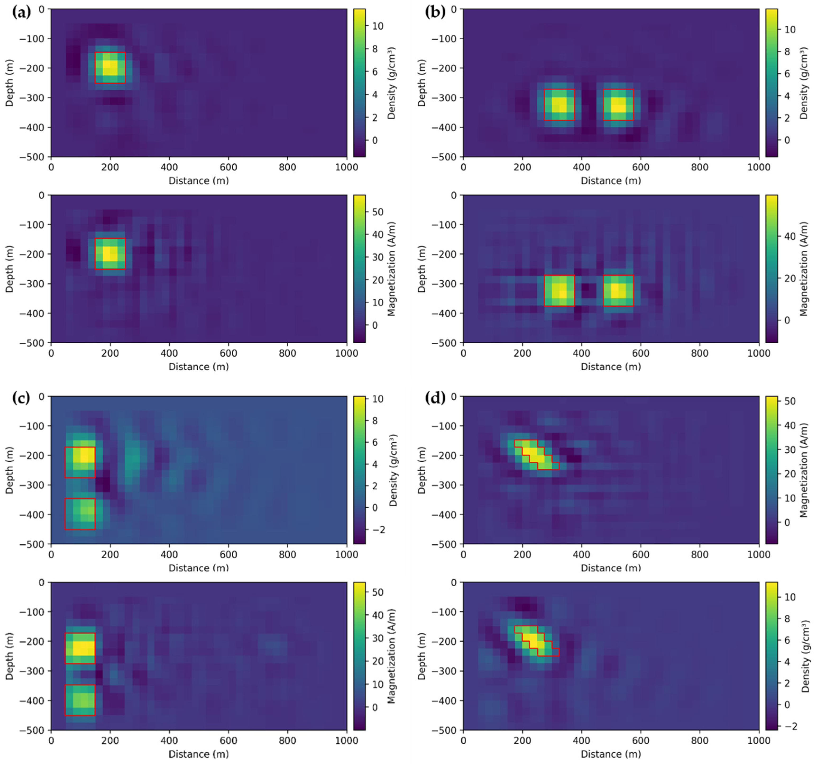
To enhance the diversity of the dataset, we categorized it into different types based on the physical properties and spatial distribution of the anomaly bodies. The anomaly bodies had a density of 10 g/cm³ and a magnetization intensity of 50 A/m. We used large physical values for the forward simulation of a large amplitude of relatively “pure metal”, so as to achieve a high sensitivity in the identification of anomalies. The purpose was to train a neural network with a stronger recognition ability. This may lead to a higher accuracy of prediction, whether an anomaly exists or not. Depending on the spatial distribution of the anomaly bodies, the subsurface models included four types: a single square anomalous body measuring 100 m in length, two horizontally distributed square anomalous bodies, each with a length of 100 m, two vertically distributed square anomalous bodies, each 100 m long, and a stepped anomalous body with 100 m lengths at the top and bottom edges. Figure 1 is an illustration of a few subsurface models.

We generated a total of 1368 data samples, with 1300 samples used for the training set and 68 samples for the validation set. These samples included 450 samples with a single rectangular anomaly, 314 samples with two rectangular anomalies distributed horizontally, 278 samples with two rectangular anomalies distributed vertically, and 326 samples with a stepped anomaly. To simulate real-world scenarios, we introduced 5% random Gaussian noise to the observed data in all samples.

2.4. Network Architecture

The fundamental principle of a CNN is to simulate the human visual system by performing convolution operations on input signals to extract features. Its basic structure comprises an input layer, convolutional layers, activation functions, pooling layers, fully connected layers, and an output layer. Through the stacking of multiple network layers, higher-level features are gradually extracted, ultimately establishing nonlinear mapping from input signals to output signals. Based on CNNs, we proposed a deep learning network model named GMNet designed for regression tasks on spatial series data. A brief schematic diagram of GMNet is presented in Figure 2. The detailed description of the GMNet architecture is as follows:

Input Layer: The model’s input layer receives two spatial series data with same sizes (101, 1). This dimension choice is based on the requirements of the problem, ensuring a proper information flow.

Convolutional and MaxPooling Layers: This is the core feature extraction part of the model. We chose a convolutional kernel size of 3, meaning each kernel considers three consecutive time steps. This kernel size selection is aimed at capturing local features in the time series, such as variations and trends. The first convolutional layer contains 32 kernels to learn various local features. Subsequent pooling layers perform 2× downsampling, reducing the dimensions of the feature maps while retaining essential information. The model includes three convolutional layers, each extracting higher-level features based on the output of the previous layer.

Flatten Layer: This layer’s role is to flatten the feature maps produced by the convolutional layers into a one-dimensional vector to input into the fully connected layers.

Dense Layers: Fully connected layers are used for further feature extraction and non-linear transformations. The model includes two fully connected layers with 256 and 128 neurons, respectively. Each neuron introduces non-linearity through the Rectified Linear Unit (ReLU) activation function (ReLU(x) = max(0,x), Jarrett et al., 2009) [30], facilitating the model’s ability to learn complex data relationships. The use of the Rectified Linear Unit (ReLU) activation function allows the model to perform nonlinear modeling and adapt to complex data patterns.

Output Layer: The output layer is used for regression tasks with a size of 800, consistent with the underlying model. Each neuron incorporates the density and magnetization intensity of the corresponding square cell. No activation function is used in the output layer because the aim is to directly output regression predictions. The design of this architecture is based on deep learning best practices and empirical knowledge, with the goal of capturing crucial features in the input data and achieving high-performance regression predictions. Careful adjustments were made to the choice of convolutional kernel sizes, the number of kernels, and the neurons in the fully connected layers to achieve a good performance without introducing excessive parameters.

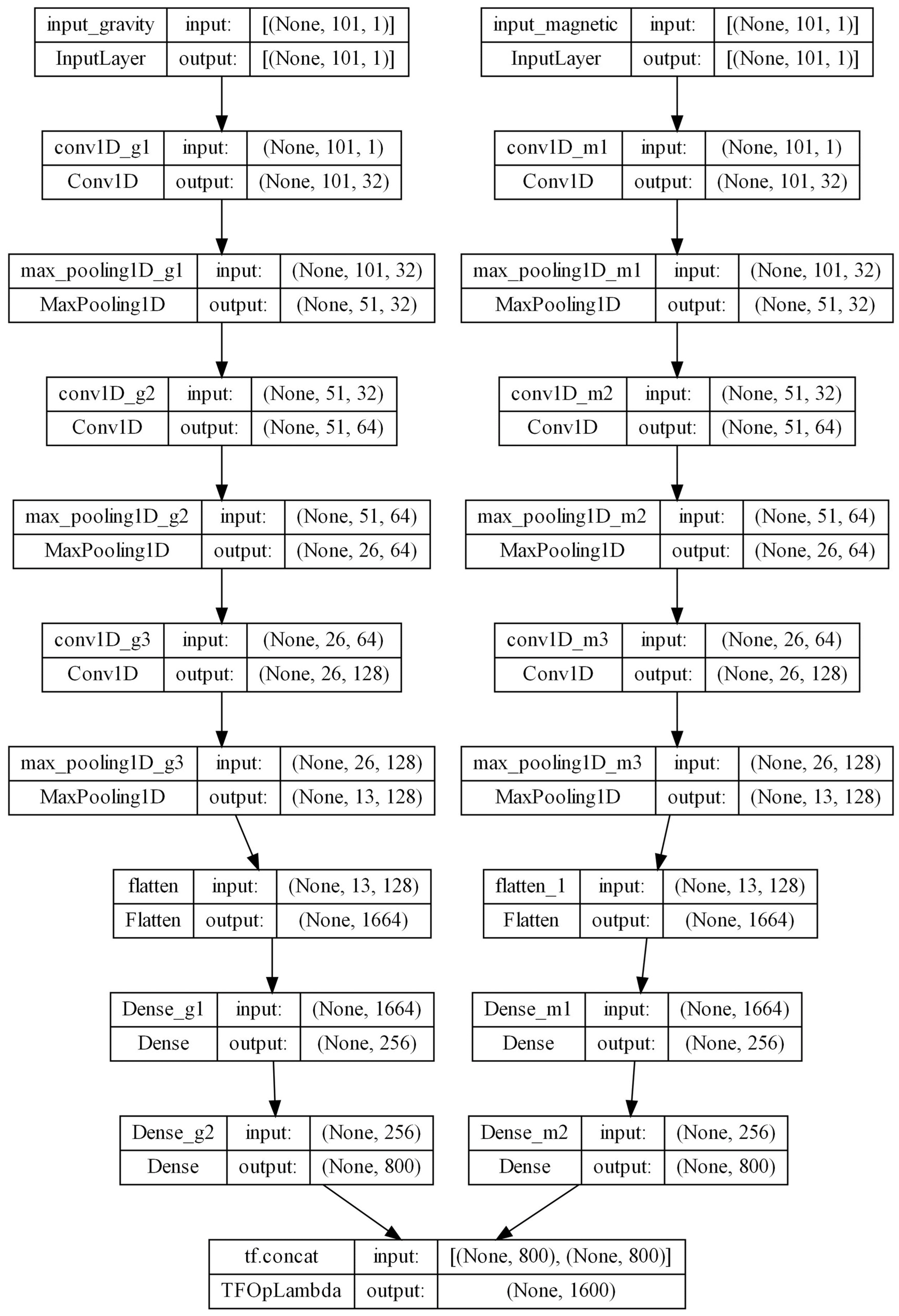
In using GMNet machine learning, the detailed architecture is shown in Figure 3. Figure 3 shows how GMNet is implemented. The model has two input layers, one for receiving gravity observations and one for magnetic observations. Each input layer is shaped (101, 1). The processing of gravity and magnetic data includes three convolutional and pooling layers, a flattening layer, and two dense layers, respectively. Finally, there is a tf.concat layer.

The first convolutional layers are conv1D_g1 and conv1D_m1, which contain 32 convolutional kernels with a convolutional kernel size of 3, an activation function of ReLU, and a filling method of ‘same’. The first pooling layers are max_pooling1D_g1 and max_pooling1D_m1, which have the maximum pooling, a pooling window size of 2, a filling method of ‘same’, and a step length of 2. Similarly, there are two convolutional layers and a pooling layer, where the second and third convolutional kernels have 64 and 128 kernels, respectively, all other parameters are the same as the first convolutional layer, and the parameters of the pooling layer are the same as those of the first pooling layer. The flattening layer flattens the feature map into a one-dimensional vector. The next two dense layers each have 256 and 800 neurons, respectively. The final tf.concat layer combines the gravity and magnet models as an output. The output of the model is a one-dimensional vector, and the inversion results in the GMNet graph are obtained after the output of the model is reshaped.

2.5. Physical Informed Loss Function

To better tailor our approach to the problem, we proposed a custom loss function $L^{\prime }$, which comprises the following two components:

$$L^{\prime }=\frac{1}{2N}{\displaystyle \sum _{i=0}^N{(u\_pre{d}_i-u\_tur{e}_i)}^2+}\frac{\lambda }{2N}{\displaystyle \sum _{i=0}^N{(d_i-Gu\_pre{d}_i)}^2},$$

(16)

where $u\_pre{d}_i$ represents the predicted values for the subsurface model, $u\_tur{e}_i$ is the true value or label for the i-th subsurface model, $\lambda$ is the weighting factor which we set to 1, d is the surface observation data, and $G$ is the operator characterized by the kernel functions for forward calculation, which includes $G_1$ and $G_2$ as shown in Equation (15). The first term of the loss function measures the mean squared error between the original predicted values and the labels, reflecting the overall model performance. The second term calculates the mean squared error between the actual surface data and the data computed based on the predictive model, which is based on the physically constrained forward modeling (e.g., gravity and magnetism). The process of generating data from the predictive model is entirely based on the physical forward calculations. Therefore, by incorporating the second term of the loss function, the network is able to capture more complex relationships. It is clear that the second term can simultaneously constrain the gravity and magnetic models to their optimal states. This addition not only enhances the accuracy of the model, but also ensures that the predictions adhere to physical laws, thereby improving the overall performance and reliability of the neural network.

The final loss function is a linear combination of these two terms, with each term having an equal weight, balancing the model’s performance. The proposed loss function introduces physical constraints into the algorithm, enabling the model to better conform to the requirements of real-world problems.

3. Synthetic Experiments

In our data inversion experiments, we employed a Convolutional Neural Network (CNN) deep learning architecture. This network was trained using 1300 training samples and evaluated for performance using 68 validation samples. To expedite convergence, we utilized the Adam optimizer with an initial learning rate of 0.01 and incorporated learning rate decay at a rate of 0.00001 to fine-tune the model parameters effectively. Following each convolutional operation, Rectified Linear Unit (ReLU) activation functions were employed to introduce non-linearity, enabling the network to better capture complex patterns and features within the data. Optimizers and activation functions play indispensable roles in neural networks. Optimizers are responsible for adjusting the network parameters to minimize the loss function, while activation functions introduce nonlinearity, enabling the network to learn and approximate complex functions. The Adam optimizer, with its adaptive learning rate characteristic, can dynamically adjust the step size of parameter updates, thereby accelerating model convergence and enhancing performance [31]. On the other hand, the ReLU activation function, with its simple and efficient computational approach and ability to alleviate gradient vanishing, enhances the expressive power of the network.

To ensure a stable training process, we partitioned the data into mini-batches, each containing 16 samples. This approach not only reduced memory consumption, but also improved training efficiency. Training was conducted over 3000 epochs. Figure 4 illustrates a selection of joint gravity and magnetic inversion results achieved by our method on the validation dataset, with the true locations of anomalies highlighted by red boxes.

In the representative inversion results presented above, we can observe that the majority of the models achieved good agreement in terms of the depth and positioning of subsurface anomalies. The inversion of anomaly density and magnetization intensity closely approximated the true values (density at 10 g/cm³ and magnetization intensity at 50 A/m). However, the delineation of anomaly boundaries was not exceptionally accurate. The inversion results of the combined model with two anomalous bodies indicate that the lateral resolution was higher than the vertical resolution, and the density and magnetization intensity in the central portion of the anomalous bodies closely matched the actual values. Moreover, the left and right positions of two adjacent anomalies were well-distinguished (Figure 4b). In the inversion of upper and lower rectangular anomalies, it was evident that the density and magnetization intensity of the upper anomaly were closer to the true values, whereas the physical properties of the lower anomaly were not as accurately retrieved (Figure 4c). This discrepancy is attributed to the strong anomaly from the shallow source overpowering the weak anomaly from the deeper source. The CNN algorithm exhibited a lower sensitivity to learning deep responses, resulting in a less accurate vertical performance compared to horizontal performance. Regarding the surrounding rocks, those located far from the anomalies exhibited density and magnetization intensity values close to zero. However, the rocks in proximity to the anomalies yielded inversion results that may slightly underestimate the true values. Figure 5 presents the variations in the loss function versus epochs during the training procedure. As can be seen from Figure 5, during the training process, the loss value generally decreased continuously, indicating a stable learning rate of the algorithm.

4. Comparison of GMNet Machine Learning Method and Cross-Gradient-Based Joint Inversion Method

4.1. Cross-Gradients

Gallardo and Meju first proposed a joint inversion method based on cross-gradient functions in 2003. Since then, it has gained significant popularity and found applications in various fields such as magnetotelluric data analysis, DC data analysis, seismic data processing, and the joint inversion of gravity and magnetic data (Gallardo and Meju, 2003; Gao and Zhang, 2018; Zhang and Wang, 2019) [10,11,32].

The three-dimensional cross-gradient function is defined as:

$$\overrightarrow{t}(m_1,m_2):=\overrightarrow{t}\left(x,y,z\right)=\nabla m_1\left(x,y,z\right)\times \nabla m_2\left(x,y,z\right).$$

(17)

In the given equation, the symbol $\nabla$ represents the gradient operator, while $m_1$ and $m_2$ are variables that denote the density and susceptibility parameters used in gravity–magnetic joint inversion. The cross-gradients criterion assumes that the problem should fulfill the condition $\overrightarrow{t}(m)=0$ ($m=(m_1,m_2)$). This condition implies that any spatial variations in both density and susceptibility should exhibit consistent directional changes, regardless of their magnitudes. In a geological context, this means that, if a boundary exists, it should be detected by both methods in a consistent orientation, irrespective of the magnitude of changes observed in the physical properties (Zhang and Wang, 2019) [11]. Taking the three-dimensional case as an example, $\overrightarrow{t}$ can be expanded in three directions:

$$t_x=\frac{\mathsf{\partial }{m}_1}{\mathsf{\partial }y}\cdot \frac{\mathsf{\partial }{m}_2}{\mathsf{\partial }z}-\frac{\mathsf{\partial }{m}_1}{\mathsf{\partial }z}\cdot \frac{\mathsf{\partial }{m}_2}{\mathsf{\partial }y},$$

(18)

$$t_y=\frac{\mathsf{\partial }{m}_1}{\mathsf{\partial }z}\cdot \frac{\mathsf{\partial }{m}_2}{\mathsf{\partial }x}-\frac{\mathsf{\partial }{m}_1}{\mathsf{\partial }x}\cdot \frac{\mathsf{\partial }{m}_2}{\mathsf{\partial }z},$$

(19)

$$t_z=\frac{\mathsf{\partial }{m}_1}{\mathsf{\partial }x}\cdot \frac{\mathsf{\partial }{m}_2}{\mathsf{\partial }y}-\frac{\mathsf{\partial }{m}_1}{\mathsf{\partial }y}\cdot \frac{\mathsf{\partial }{m}_2}{\mathsf{\partial }x}.$$

(20)

If we consider a two-dimensional model, the partial derivative of the model with respect to the $y$-axis direction becomes zero. In this scenario, the two-dimensional cross-gradient function is defined as follows:

$$\overrightarrow{t}(m_1,m_2):=\overrightarrow{t}\left(x,z\right)=\nabla m_1(x,z)\times \nabla m_2(x,z).$$

(21)

In which, the mathematical symbol “:=” refers to “defined by”. In this situation, with the expansion of $\overrightarrow{t}$, only $t_y$ remains.

The above cross-gradient function is initially defined in a continuous form, requiring discretization for practical inversion calculations. In this study, we employ the finite difference method to discretize the cross-gradient function using a seven-point central stencil.

The cross-gradient function involves gradient and cross-product operations that possess the following characteristics:

(1)

The gradient of a point within the scalar field indicates the direction of fastest growth, with its magnitude signifying the rate of change in the scalar field at that point;

(2)

The cross-product of two vectors equals the product of their magnitudes multiplied by sinθ, where θ represents the angle between the two vectors. When the two vectors are parallel, resulting in an angle of 0 or 180 degrees, and sinθ becomes zero, the cross-product equates to zero as well.

By incorporating the aforementioned properties into geophysical joint inversion, the following observations can be made:

(1)

If both physical parameters involved in the joint inversion change in the same direction, or if one physical parameter remains unchanged, the cross-gradient function assumes a value of zero.

(2)

Conversely, when the gradient of the two physical parameters is not parallel, the cross-gradient function does not equal zero.

These properties serve as the fundamental basis for geophysical joint inversion utilizing the cross-gradient function.

4.2. Comparison of Cross-Gradients-Based Inversion with GMNet Inversion

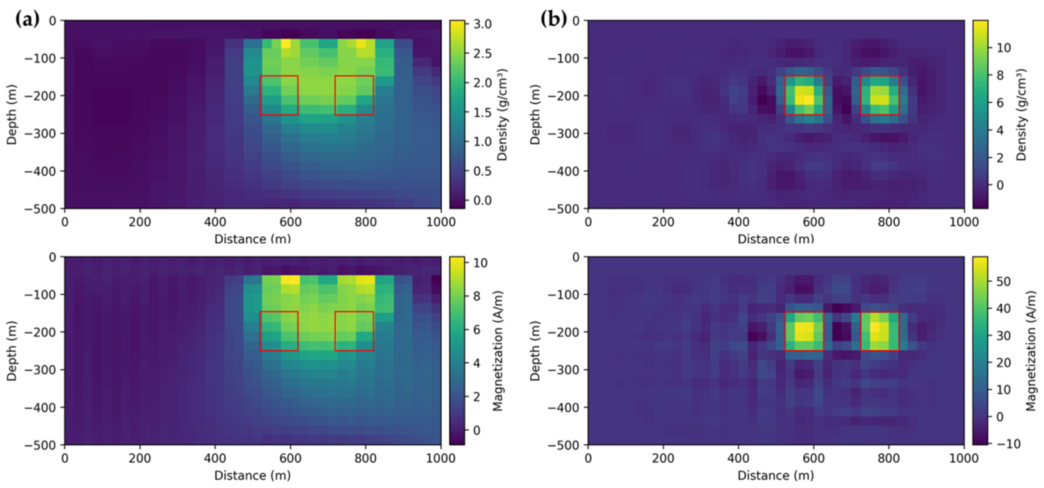
To assess the inversion performance of the GMNet-based joint inversion method for gravity and magnetic fields, we applied the method to invert an underground model featuring two anomalous bodies with a density of 10 g/cm³ and a magnetization intensity of 50 A/m. A comparative analysis was conducted with the results obtained from the gravity and magnetic cross-gradient joint inversion method, a purely model-based joint inversion algorithm. In our implementation, we utilized only its two-dimensional form, extending the underground model region and the number of anomalous bodies. The initial inversion model was set as an underground space with a density of 1 g/cm³ and a magnetization intensity of 1 A/m. We performed 300 iterations, taking approximately 5 min. Figure 6 illustrates the inversion results of the two methods, with the true position of the anomalous body marked by a red box. Figure 6a displays the inversion results obtained using the cross-gradient-based joint inversion method, while Figure 6b presents the results obtained using the GMNet machine learning method. The first method yielded inversion results with lower density and magnetization values than the true values, accompanied by a blurred position of the anomalous body. In contrast, the second method demonstrated effective inversion results in less than a second. Data-driven methods, such as GMNet, exhibit the advantage of not requiring an initial inversion model and can achieve superior inversion results with minimal computational time.

5. Testing Model Inversion

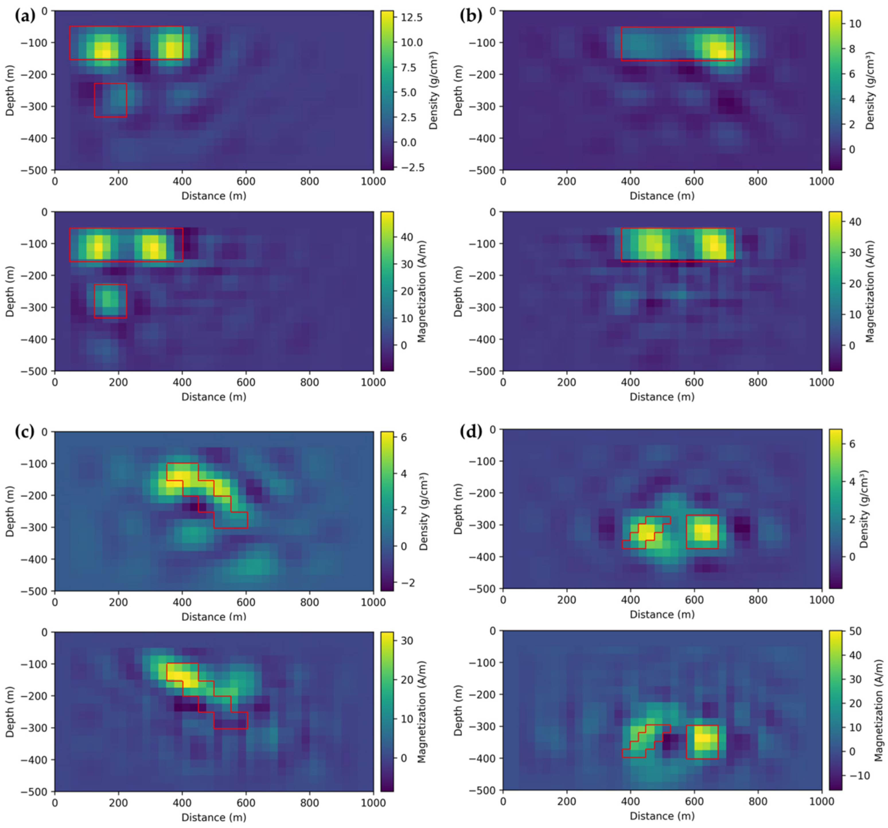
Since the data used for prediction in the previous section were extracted from a total of 1368 generated data samples, the prediction set shared similarities with the training set. In order to evaluate the neural networks’ generalization capability, we further designed several subsurface models that significantly differed from the original data, generating corresponding field data. These differences were primarily manifested in the shapes and spatial distribution of the anomalous bodies. Figure 7 presents representative inversion results of the gravity and magnetic field data for these diverse scenarios.

It can be observed that the inversion results for the newly designed subsurface models are not ideal. However, we can still make approximate determinations about the positions of the anomalous bodies. Due to the absence of similar training samples, the network may mistakenly identify a rectangular anomaly as two square anomalies (Figure 7a,b) or misinterpret a stepped anomaly as a layer similar to an anticlinal structure (Figure 7c). Moreover, the issue of inadequate vertical resolution is more pronounced. In the new inversion results, we can observe that many density and magnetization intensity values for surrounding rocks are were zero, which is inaccurate. This also implies that when the training samples for the network are insufficient, the predicted results are likely to be incorrect. The density and magnetization intensities of the anomalies were close to their true values. This model demonstrated strong learning and generalization capabilities.

6. Field Example

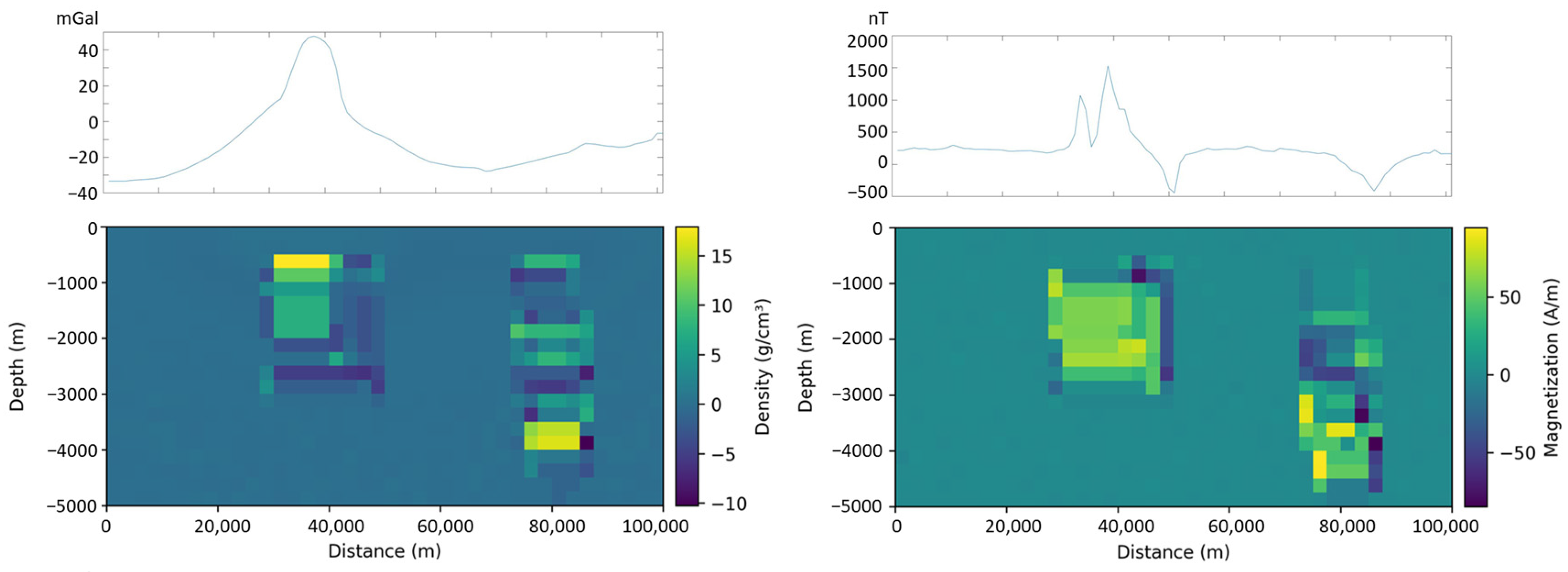
The actual data used in this study are from the central–southern region of Jussara, Goias State, Brazil. The Bouguer gravity anomaly and total magnetic anomaly of the region are depicted in Figure 8. We selected the observation data from traverse line AB for inversion using the GMNet machine learning method. Traverse line AB is approximately 10,000 m long, and due to the limited number of measurement points, we interpolated it to obtain 101 observation points spaced at 100 m intervals. These data were processed to meet the requirements of GMNet. The network architecture and parameter settings remained the same as before. Considering the various uncertainties in real data, and to mitigate the impact of underground model parameter variations on the inversion results, we modified the training samples used for network training. We extended the previously used 1300 training samples to a larger subsurface space, with a length of 100,000 m and a depth of 5000 m. Similarly, the underground two-dimensional space was set as 800 (20 rows × 40 columns) rectangular cells, but each cell had a length of 2500 m. The distribution and shape of these samples did not change significantly. In addition, to enhance the accuracy of the inversion results, we generated 640 additional sample sets with the same scale of the samples intended for the prediction for network training. The training time was approximately 30 min, and the prediction time was less than 1 s.

Figure 9 presents the inversion results of transverse line AB using GMNet. The results indicate the presence of two anomalous bodies along the profile. The anomalous body to the west has a burial depth of approximately 1000 m, while the one to the east is buried at around 4000 m. The positions of these anomalous bodies correspond well with the peak values of the field anomalies along traverse line AB. The boundaries of the anomalous bodies are not distinct, and there are noticeable low-value regions near the boundaries. The inversion values for the density and magnetization of anomalous bodies may be high, leading to higher observed values compared to the real values. So, the low-value regions possibly represent a compromise made by the network to fit the real anomaly values. Constrained by the limitations of machine learning inversion methods, the inversion results may not precisely reflect the true underground model.

As a comparison, if we directly inverted real data using the model trained in Section 3, the results would be unsatisfactory and may be erroneous. This phenomenon could be attributed to a significant disparity between training sets for subsurface regions and predicted regions (training sets for subsurface regions: 1000 × 500; predicted subsurface regions: 100,000 × 5000). This is reason why we added 640 additional sample sets with the same scale of the region intended for the prediction for network training. Therefore, the predictive capability of the network is highly dependent on appropriate training samples, as inappropriate training samples may result in erroneous conclusions. In conclusion, inversion methods based on machine learning still hold significant potential.

7. Conclusions

Improving the reliability of inversion results is a hot topic in the field of geophysics. In this research, we propose a novel approach to jointly invert gravity and magnetic field data using Convolutional Neural Networks (CNNs). This data-driven method provides a new perspective for addressing geophysical inversion problems, relying primarily on data-driven training, rather than traditional methods that heavily depend on prior knowledge and assumptions. By simulating the forward modeling of gravity and magnetic fields, we generated a large-scale dataset for training the CNN model. We constructed a CNN network for the joint inversion of gravity and magnetic data. To enhance the convergence rate, we employed the Adam optimizer and used Rectified Linear Unit (ReLU) as the activation function during network training.

Compared to traditional inversion methods, deep learning is a data-driven process that does not require dealing with non-uniqueness. However, one potential limitation is that it may not adequately capture the complexity and heterogeneity of solutions when training data are scarce. To address this, we introduced a custom loss function, providing the network with physical interpretability to prevent over-reliance on data-driven training, thus making it more robust for gravity and magnetic field inversion problems. Once the model is trained, the prediction time for the distribution and physical properties of subsurface anomalies becomes negligible.

In the synthetic data validation experiments, the network’s inversion results were also quite promising. The network exhibited strong learning and generalization capabilities, even for the newly designed subsurface models. However, when the training samples are insufficient, this method may lead to incorrect conclusions. In the section involving field data, the method also provided predictive results for the subsurface model. In summary, machine-learning-based inversion methods exhibit significant potential, offering valuable insights into the detection of subsurface ore bodies and guiding subsequent drilling activities.

References

1. Zhdanov, M.S. Geophysical Inverse Theory and Regularization Problems; Elsevier: Amsterdam, The Netherlands, 2002. [Google Scholar]
2. Zeng, H.L. Gravity Field and Gravity Exploration; Geological Press: Beijing, China, 2005. [Google Scholar]
3. Guan, Z.N. Geomagnetic Field and Magnetic Exploration; Geological Press: Beijing, China, 2005. [Google Scholar]
4. Phillips, N.D. Geophysical Inversion in an Integrated Exploration Program: Examples from the San Nicolas Deposit. Master’s Thesis, University of British Columbia, Vancouver, BC, Canada, 2001. [Google Scholar]
5. Lane, R.; FitzGerald, D.; Guillen, A.; Seikel, R.; Mclnerey, P. Lithologically constrained inversion of magnetic and gravity data sets. In Proceedings of the 10th SAGA Biennial Technical Meeting and Exhibition, Wild Coast, South Africa, 22–26 October 2007; Volume 129, pp. 11–17. [Google Scholar]
6. Farquharson, C.G.; Ash, M.R.; Miller, H.G. Geologically constrained gravity inversion for the Voisey’s Bay ovoid deposit. Lead. Edge 2008, 27, 64–69. [Google Scholar] [CrossRef]
7. Williams, N.C. Geologically-Constrained UBC-GIF Gravity and Magnetic Inversions with Examples from the Agnew-Wiluna Greenstone Belt, Western Australia. Ph.D. Thesis, University of British Columbia, Vancouver, BC, Canada, 2008. [Google Scholar]
8. Lelièvre, P.G. Integrating Geologic and Geophysical Data through Advanced Constrained Inversions. Ph.D. Thesis, University of British Columbia, Vancouver, BC, Canada, 2009. [Google Scholar]
9. Moorkamp, M.; Heincke, B.; Jegen, M.; Hobbs, R.; Henderson, D. Joint inversion of MT, gravity and seismic data applied to sub-basalt imaging. In Proceedings of the International Workshop on Electromagnetic Induction in the Earth, Beijing, China, 23–29 October 2008. [Google Scholar]
10. Gallardo, L.A.; Meju, M.A. Characterization of heterogeneous near-surface materials by joint 2D inversion of dc resistivity and seismic data. Geophys. Res. Lett. 2003, 30, 183–196. [Google Scholar] [CrossRef]
11. Zhang, Y.P.; Wang, Y.F. Three-dimensional gravity-magnetic cross-gradient joint inversion based on structural coupling and a fast gradient method. J. Comput. Math. 2019, 37, 758–777. [Google Scholar]
12. Sun, J.; Li, Y. Multidomain petrophysically constrained inversion and geology differentiation using guided fuzzy c-means clustering. Geophysics 2015, 80, ID1–ID181. [Google Scholar] [CrossRef]
13. Samuel, A.L. Some studies in machine learning using the game of checkers. IBM J. Res. Dev. 1959, 3, 210–229. [Google Scholar] [CrossRef]
14. Mitchell, T.M. Machine Learning; McGraw-Hill Higher Education: New York, NY, USA, 1997. [Google Scholar]
15. Dowla, F.U.; Taylor, S.R.; Anderson, R.W. Seismic discrimination with artificial neural networks: Preliminary results with regional spectral data. Bull. Seismol. Soc. Am. 1990, 80, 1346–1373. [Google Scholar]
16. Zhao, X.; Mendel, J.M. 1988. Minimum-variance deconvolution using artificial neural networks. In SEG Technical Program Expanded Abstracts; Society of Exploration Geophysicists: Houston, TX, USA, 1988; pp. 738–741. [Google Scholar]
17. Li, J.; Liu, Y.; Yin, C.; Ren, X.; Su, Y. Fast imaging of time-domain airborne EM data using deep learning technology. Geophysics 2020, 85, E163–E170. [Google Scholar] [CrossRef]
18. Moghadas, D. One-dimensional deep learning inversion of electromagnetic induction data using convolutional neural network. Geophys. J. Int. 2020, 222, 247–259. [Google Scholar] [CrossRef]
19. Wu, B.; Meng, D.; Wang, L.; Liu, N.; Wang, Y. Seismic impedance inversion using fully convolutional residual network and transfer learning. IEEE Geosci. Remote Sens. Lett. 2020, 17, 1–5. [Google Scholar] [CrossRef]
20. Nurindrawati, F.; Sun, J. Predicting magnetization directions using convolutional neural networks. J. Geophys. Res. Solid Earth 2020, 125, e2020JB019675. [Google Scholar] [CrossRef]
21. Li, Y.; Yang, D. Electrical imaging of hydraulic fracturing fluid using steel-cased wells and a deep-learning method. Geophysics 2021, 86, E315–E332. [Google Scholar] [CrossRef]
22. He, S.; Cai, H.; Liu, S.; Xie, J.; Hu, X. Recovering 3D Basement Relief Using Gravity Data Through Convolutional Neural Networks. J. Geophys. Res. Solid Earth 2021, 126, e2021JB022611. [Google Scholar] [CrossRef]
23. Huang, R.; Liu, S.; Qi, R.; Zhang, Y. Deep learning 3D sparse inversion of gravity data. J. Geophys. Res. Solid Earth 2021, 126, e2021JB022476. [Google Scholar] [CrossRef]
24. Yang, Q.; Hu, X.; Liu, S.; Jie, Q.; Wang, H.; Chen, Q. 3-D gravity inversion based on deep convolution neural networks. IEEE Geosci. Remote Sens. Lett. 2021, 19, 1–5. [Google Scholar] [CrossRef]
25. Zhang, L.; Zhang, G.; Liu, Y.; Fan, Z. Deep learning for 3-D inversion of gravity data. IEEE Trans. Geosci. Remote Sens. 2021, 60, 1–18. [Google Scholar] [CrossRef]
26. Bergen, K.J.; Johnson, P.A.; Maarten, V.; Beroza, G.C. Machine learning for data-driven discovery in solid Earth geoscience. Science 2019, 363, eaau0323. [Google Scholar] [CrossRef] [PubMed]
27. Wang, Y.F.; Volkov, V.T.; Yagola, A.G. Basic Theory of Inverse Problems: Variational Analysis and Geoscience Applications; Science Press: Beijing, China, 2021. [Google Scholar]
28. Wang, Y.F.; Zou, A.Q. Regularization and optimization methods for micro pore structure analysis of shale based on neural networks. Acta Petrol. Sin. 2018, 34, 281–288. [Google Scholar]
29. Yang, F.; Ma, J. Deep-learning inversion: A next-generation seismic velocity model building method. Geophysics 2019, 84, R583–R599. [Google Scholar] [CrossRef]
30. Kevin, J.; Koray, K.; Marc’Aurelio, R.; Yann, L. What is the best multi-stage architecture for object recognition? In Proceedings of the IEEE 12th International Conference on Computer Vision, Kyoto, Japan, 27 September–4 October 2009. [Google Scholar] [CrossRef]
31. Kingma, D.P.; Ba, J. Adam: A method for stochastic optimization. arXiv 2014. [Google Scholar] [CrossRef]
32. Gao, J.; Zhang, H.J. An efficient sequential strategy for realizing cross-gradient joint inversion: Method and its application to two-dimensional cross borehole seismic travel time and DC resistivity tomography. Geophys. J. Int. 2018, 213, 1044–1055. [Google Scholar]
Figure 1. Training set samples with anomaly bodies with density of 10 g/cm3 and a magnetization intensity of 50 A/m, (a) single rectangular anomaly body, (b) two rectangular anomaly bodies distributed horizontally, (c) two rectangular anomaly bodies distributed vertically, and (d) one stepped anomaly body.
Remotesensing 16 01115 g001
Figure 2. Gravity–magnetic inversion net (GMNet).
Remotesensing 16 01115 g002
Figure 3. Network architecture schematic.
Remotesensing 16 01115 g003
Figure 4. Joint gravity and magnetic inversion results, where the true positions of the anomalous bodies are marked by a red box. (a) single rectangular anomaly body, (b) two rectangular anomaly bodies distributed from left to right, (c) two rectangular anomaly bodies distributed from top to bottom, and (d) one-stepped anomaly body.
Remotesensing 16 01115 g004
Figure 5. Loss curve for training sets.
Remotesensing 16 01115 g005
Figure 6. Joint gravity and magnetic inversion results, where the true positions of the anomalous bodies are marked by a red box. (a) cross-gradient-based joint inversion method and (b) GMNet machine learning method.
Remotesensing 16 01115 g006
Figure 7. Joint inversion results with gravity and magnetic fields data for complex models, where the true positions of the anomalous bodies are marked by a red box. (a) two rectangular anomaly bodies distributed from top to bottom, (b) single rectangular anomaly body, (c) one stepped anomaly body, and (d) one-stepped anomaly body and one rectangular anomaly body.
Remotesensing 16 01115 g007
Figure 8. Bouguer gravity anomaly and total magnetic anomaly of research region and the line AB is an east-west-direction observation line (X axis refers east orientation, Y axis refers to north orientation).
Remotesensing 16 01115 g008
Figure 9. Inversion results using GMNet machine learning method of the line AB observation and corresponding gravity and magnetic anomaly data.
Remotesensing 16 01115 g009
Disclaimer/Publisher’s Note: The statements, opinions and data contained in all publications are solely those of the individual author(s) and contributor(s) and not of MDPI and/or the editor(s). MDPI and/or the editor(s) disclaim responsibility for any injury to people or property resulting from any ideas, methods, instructions or products referred to in the content.