
TENet: A Texture-Enhanced Network for Intertidal Sediment and Habitat Classification in Multiband PolSAR Images


Abstract
1. Introduction
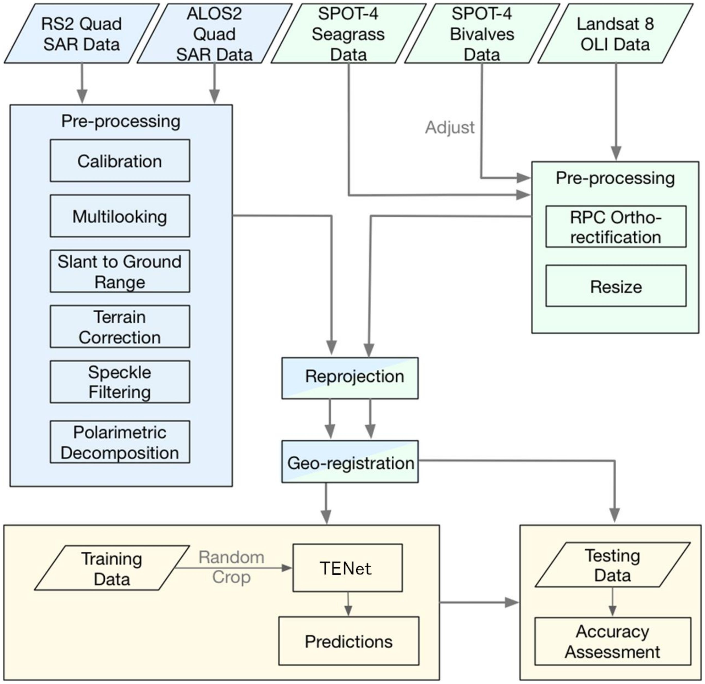
2. System Architecture
2.1. Processing Procedure
2.2. SAR Polarimetric Decomposition
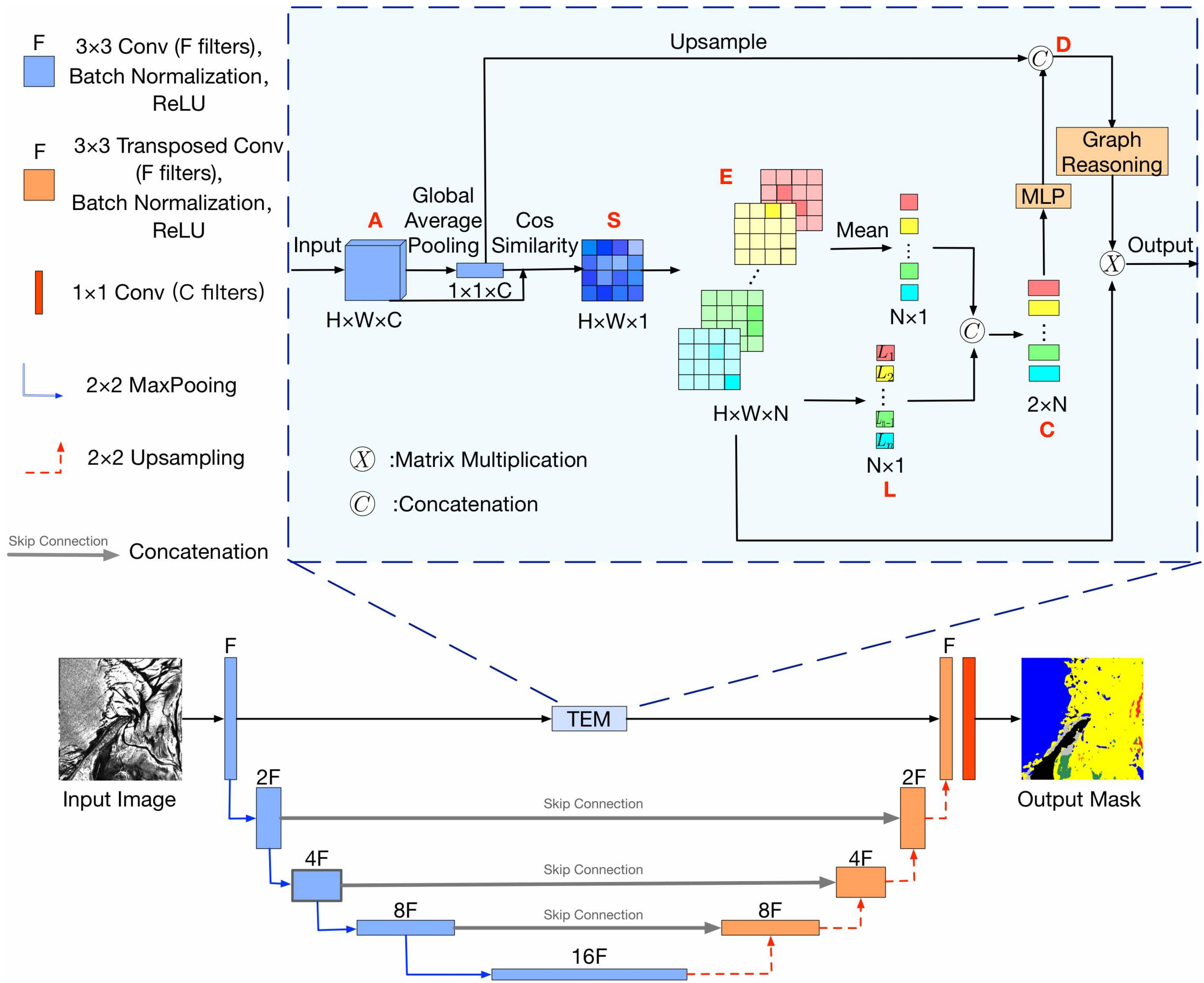
2.3. Texture Enhancement UNet
2.3.1. The Overall Architecture
2.3.2. Texture Enhancement Module
3. Dataset
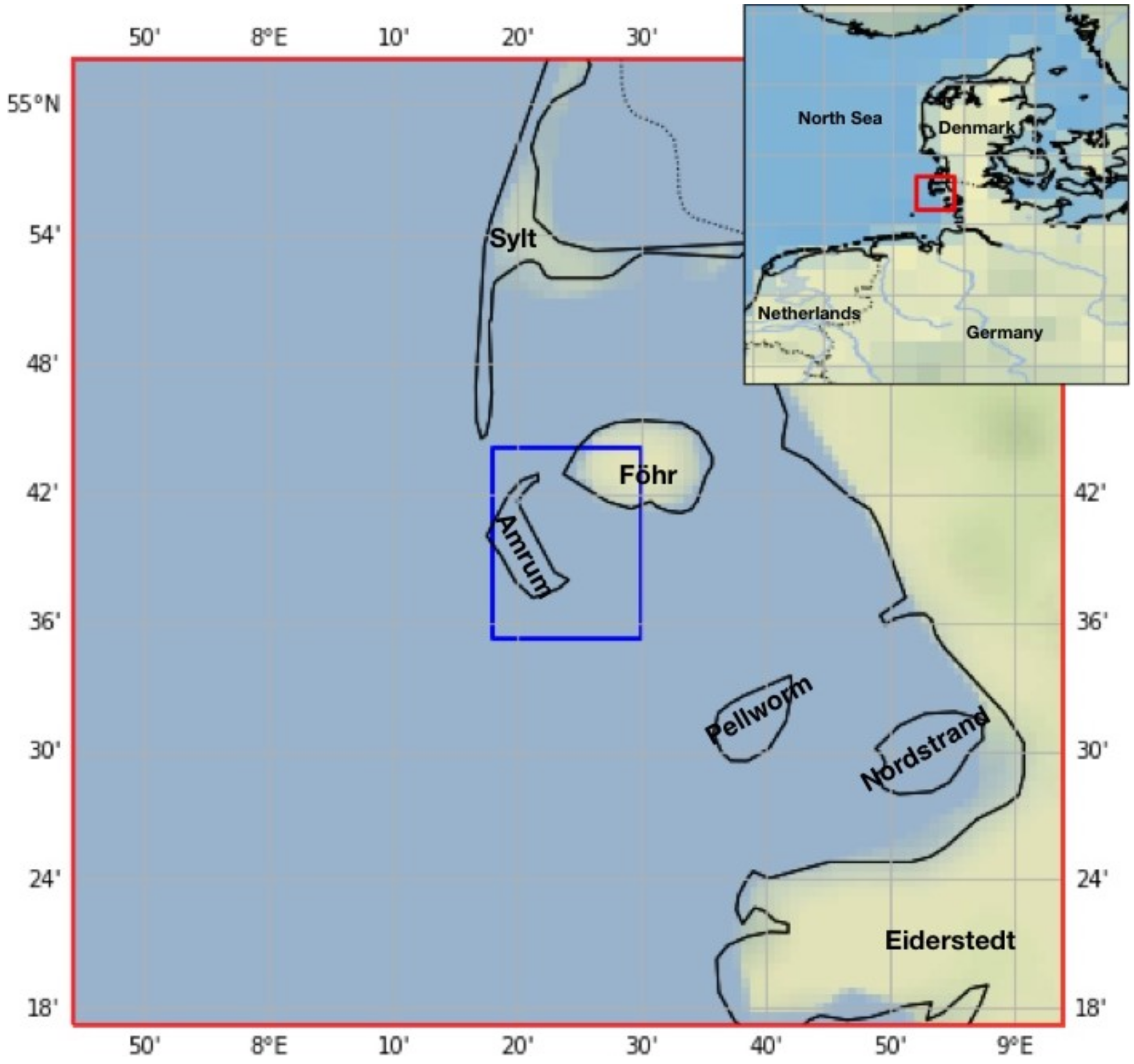
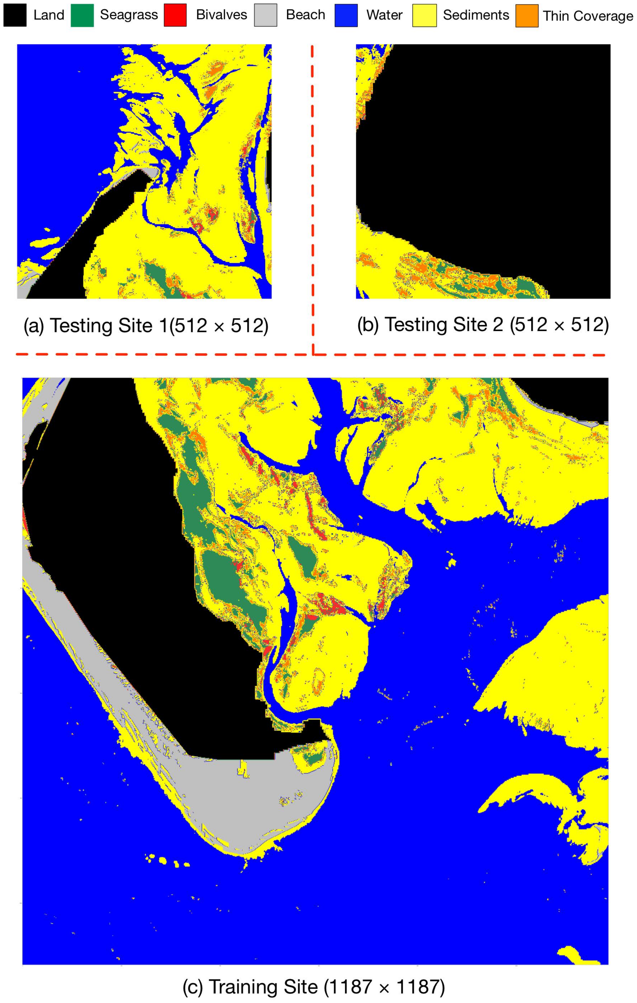
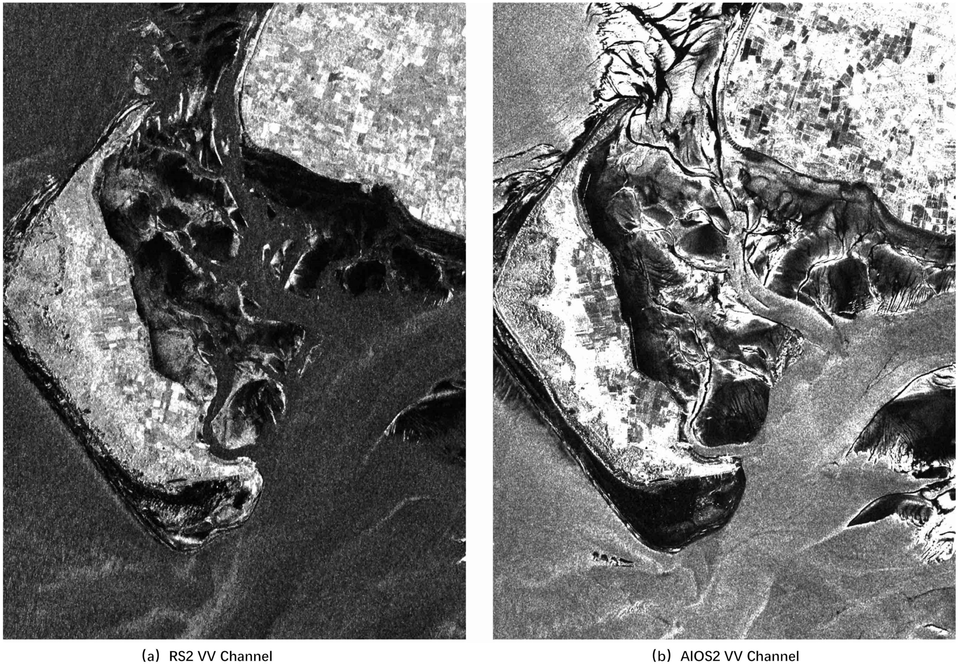
3.1. Study Area
3.2. PolSAR Data
4. Experiments
4.1. Experimental Setup
4.2. Evaluation Metrics
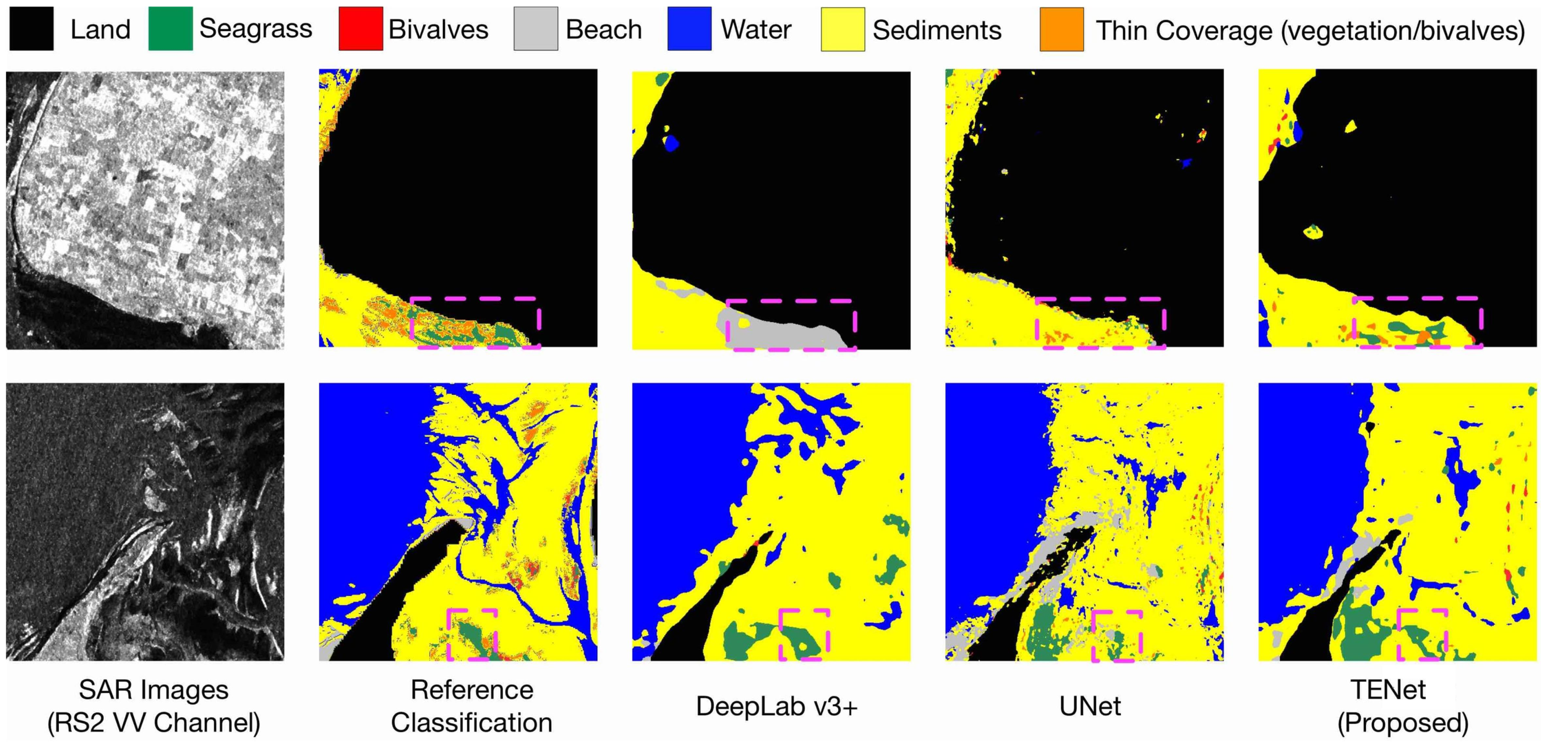
4.3. Comparison of Results
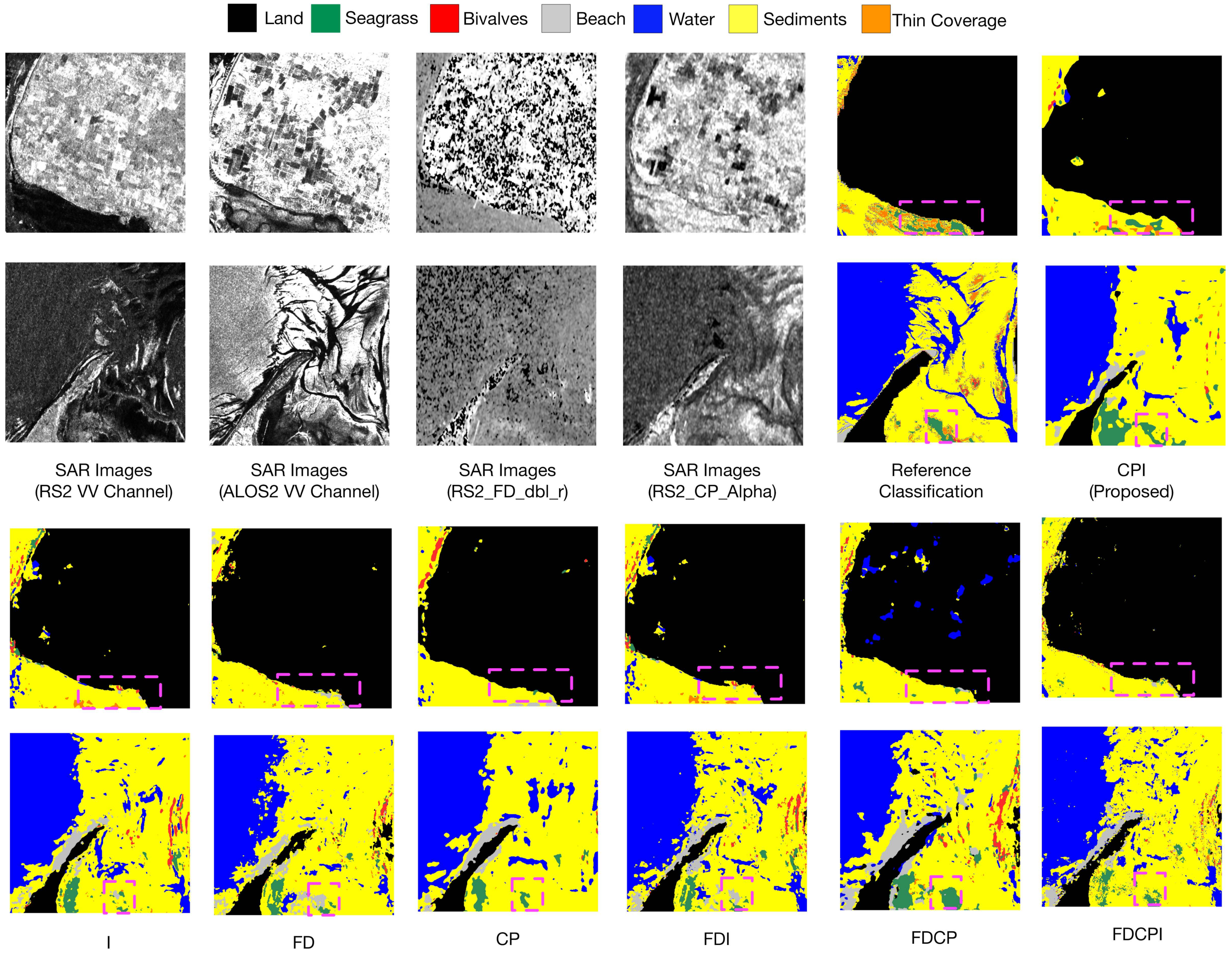
4.4. Ablation Study
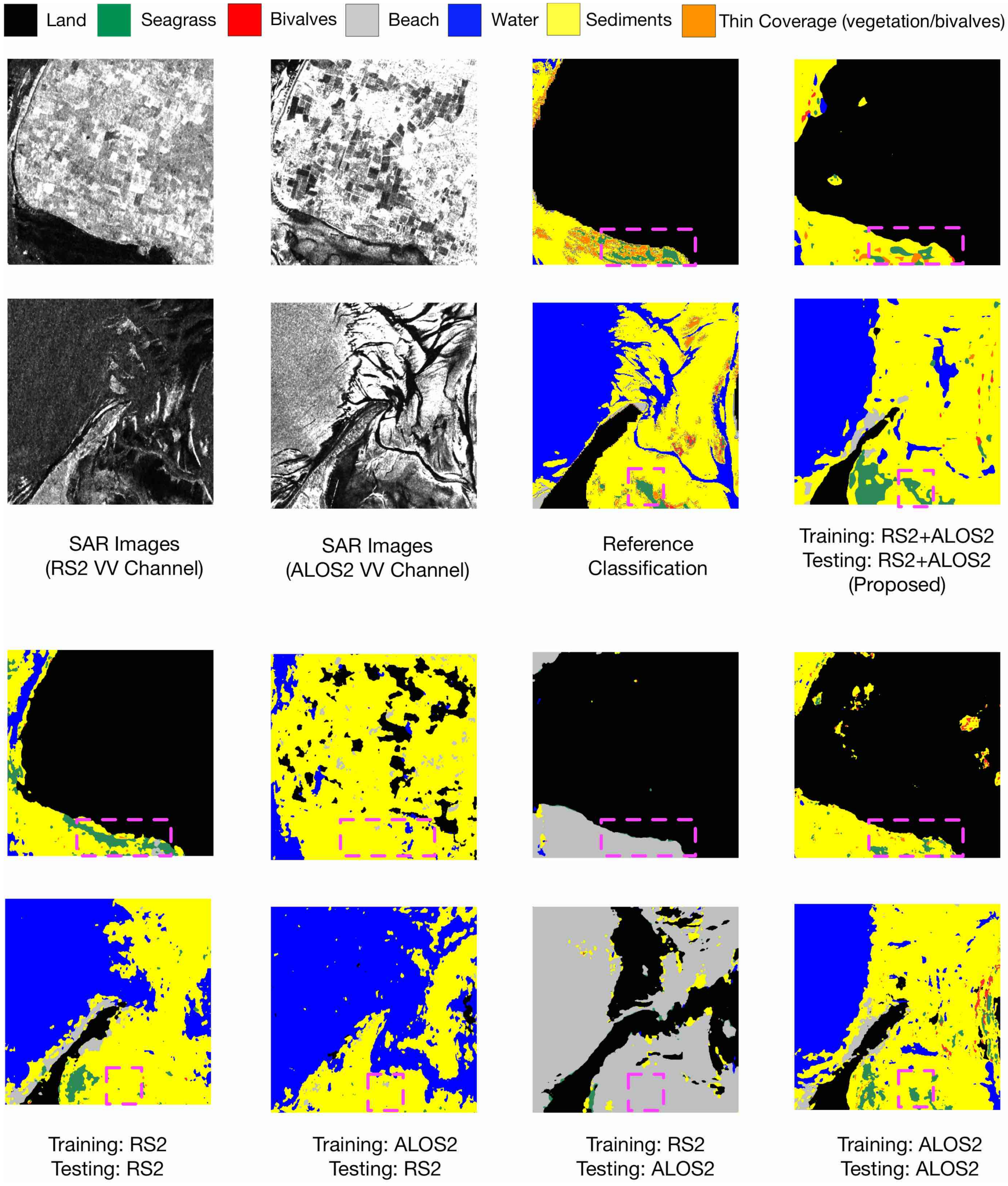
4.4.1. Multiband Input
4.4.2. Multipolarization Input
5. Discussion
6. Conclusions
Author Contributions
Funding
Data Availability Statement
Acknowledgments
Conflicts of Interest
References
- Lv, M.; Luan, X.; Liao, C.; Wang, D.; Liu, D.; Zhang, G.; Jiang, G.; Chen, L. Human impacts on polycyclic aromatic hydrocarbon distribution in Chinese intertidal zones. Nat. Sustain. 2020, 3, 878–884. [Google Scholar] [CrossRef]
- Murray, N.J.; Phinn, S.P.; Fuller, R.A.; DeWitt, M.; Ferrari, R.; Johnston, R.; Clinton, N.; Lyons, M.B. High-resolution global maps of tidal flat ecosystems from 1984 to 2019. Sci. Data 2022, 9, 542. [Google Scholar] [CrossRef]
- Bishop-Taylor, R.; Sagar, S.; Lymburner, L.; Beaman, R.J. Between the tides: Modelling the elevation of Australia’s exposed intertidal zone at continental scale. Estuar. Coast. Shelf Sci. 2019, 223, 115–128. [Google Scholar] [CrossRef]
- Nizam, A.; Meera, S.P.; Kumar, A. Genetic and molecular mechanisms underlying mangrove adaptations to intertidal environments. iScience 2022, 25, 103547. [Google Scholar] [CrossRef]
- Chmura, G.L.; Anisfeld, S.C.; Cahoon, D.R.; Lynch, J.C. Global carbon sequestration in tidal, saline wetland soils. Glob. Biogeochem. Cycles 2003, 17, 22. [Google Scholar] [CrossRef]
- Billerbeck, M.; Werner, U.; Bosselmann, K.; Walpersdorf, E.; Huettel, M. Nutrient release from an exposed intertidal sand flat. Mar. Ecol. Prog. Ser. 2006, 316, 35–51. [Google Scholar] [CrossRef]
- Smolders, S.; Plancke, Y.; Ides, S.; Meire, P.; Temmerman, S. Role of intertidal wetlands for tidal and storm tide attenuation along a confined estuary: A model study. Nat. Hazards Earth Syst. Sci. 2015, 15, 1659–1675. [Google Scholar] [CrossRef]
- Chen, Y.; Jiang, H.; Li, C.; Jia, X.; Ghamisi, P. Deep Feature Extraction and Classification of Hyperspectral Images Based on Convolutional Neural Networks. IEEE Trans. Geosci. Remote Sens. 2016, 54, 6232–6251. [Google Scholar] [CrossRef]
- Navedo, J.G.; Herrera, A.G. Effects of recreational disturbance on tidal wetlands: Supporting the importance of undisturbed roosting sites for waterbird conservation. J. Coast. Conserv. 2012, 16, 373–381. [Google Scholar] [CrossRef]
- Murray, N.J.; Phinn, S.R.; DeWitt, M.; Ferrari, R.; Johnston, R.; Lyons, M.B.; Clinton, N.; Thau, D.; Fuller, R.A. The global distribution and trajectory of tidal flats. Nature 2019, 565, 222–225. [Google Scholar] [CrossRef]
- Gade, M.; Wang, W.; Kemme, L. On the imaging of exposed intertidal flats by single- and dual-co-polarization Synthetic Aperture Radar. Remote Sens. Environ. 2018, 205, 315–328. [Google Scholar] [CrossRef]
- Wang, W.; Gade, M.; Stelzer, K.; Kohlus, J.; Zhao, X.; Fu, K. A Classification Scheme for Sediments and Habitats on Exposed Intertidal Flats with Multi-Frequency Polarimetric SAR. Remote Sens. 2021, 13, 360. [Google Scholar] [CrossRef]
- Castaneda-Guzman, M.; Mantilla-Saltos, G.; Murray, K.A.; Settlage, R.; Escobar, L.E. A database of global coastal conditions. Sci. Data 2021, 8, 304. [Google Scholar] [CrossRef] [PubMed]
- Vitousek, S.; Buscombe, D.; Vos, K.; Barnard, P.L.; Ritchie, A.C.; Warrick, J.A. The future of coastal monitoring through satellite remote sensing. Camb. Prisms Coast. Futur. 2023, 1, e10. [Google Scholar] [CrossRef]
- Brockmann, C.; Stelzer, K. Optical Remote Sensing of Intertidal Flats. In Remote Sensing of the European Seas; Barale, V., Gade, M., Eds.; Springer: Dordrecht, The Netherlands, 2008; pp. 117–128. [Google Scholar] [CrossRef]
- González, C.J.; Torres, J.R.; Haro, S.; Gómez-Enri, J.; Álvarez, Ó. High-resolution characterization of intertidal areas and lowest astronomical tidal surface by use of Sentinel-2 multispectral imagery and hydrodynamic modeling: Case-study in Cadiz Bay (Spain). Sci. Total Environ. 2023, 861, 160620. [Google Scholar] [CrossRef]
- Liu, G.; Liu, B.; Zheng, G.; Li, X. Environment Monitoring of Shanghai Nanhui Intertidal Zone With Dual-Polarimetric SAR Data Based on Deep Learning. IEEE Trans. Geosci. Remote Sens. 2022, 60, 4208918. [Google Scholar] [CrossRef]
- Hughes, M.G.; Glasby, T.M.; Hanslow, D.J.; West, G.J.; Wen, L. Random Forest Classification Method for Predicting Intertidal Wetland Migration Under Sea Level Rise. Front. Environ. Sci. 2022, 10, 749950. [Google Scholar] [CrossRef]
- Davies, B.F.R.; Gernez, P.; Geraud, A.; Oiry, S.; Rosa, P.; Zoffoli, M.L.; Barillé, L. Multi- and hyperspectral classification of soft-bottom intertidal vegetation using a spectral library for coastal biodiversity remote sensing. Remote Sens. Environ. 2023, 290, 113554. [Google Scholar] [CrossRef]
- Chun Liu, C.L.; Junjun Yin, J.Y.; Jian Yang, J.Y. Application of deep learning to polarimetric SAR classification. In Proceedings of the IET International Radar Conference 2015, Hangzhou, China, 14–16 October 2015; p. 4. [Google Scholar] [CrossRef]
- Zhang, L.; Zhang, L.; Du, B. Deep Learning for Remote Sensing Data: A Technical Tutorial on the State of the Art. IEEE Geosci. Remote Sens. Mag. 2016, 4, 22–40. [Google Scholar] [CrossRef]
- Zhu, X.X.; Tuia, D.; Mou, L.; Xia, G.S.; Zhang, L.; Xu, F.; Fraundorfer, F. Deep Learning in Remote Sensing: A Comprehensive Review and List of Resources. IEEE Geosci. Remote Sens. Mag. 2017, 5, 8–36. [Google Scholar] [CrossRef]
- Liu, X.; Jiao, L.; Tang, X.; Sun, Q.; Zhang, D. Polarimetric Convolutional Network for PolSAR Image Classification. IEEE Trans. Geosci. Remote Sens. 2019, 57, 3040–3054. [Google Scholar] [CrossRef]
- Campos-Taberner, M.; García-Haro, F.J.; Martínez, B.; Izquierdo-Verdiguier, E.; Atzberger, C.; Camps-Valls, G.; Gilabert, M.A. Understanding deep learning in land use classification based on Sentinel-2 time series. Sci. Rep. 2020, 10, 17188. [Google Scholar] [CrossRef]
- Garg, R.; Kumar, A.; Bansal, N.; Prateek, M.; Kumar, S. Semantic segmentation of PolSAR image data using advanced deep learning model. Sci. Rep. 2021, 11, 15365. [Google Scholar] [CrossRef]
- Wang, P.; Bayram, B.; Sertel, E. A comprehensive review on deep learning based remote sensing image super-resolution methods. Earth-Sci. Rev. 2022, 232, 104110. [Google Scholar] [CrossRef]
- Cui, X.; Yang, F.; Wang, X.; Ai, B.; Luo, Y.; Ma, D. Deep learning model for seabed sediment classification based on fuzzy ranking feature optimization. Mar. Geol. 2021, 432, 106390. [Google Scholar] [CrossRef]
- Tallam, K.; Nguyen, N.; Ventura, J.; Fricker, A.; Calhoun, S.; O’Leary, J.; Fitzgibbons, M.; Robbins, I.; Walter, R.K. Application of Deep Learning for Classification of Intertidal Eelgrass from Drone-Acquired Imagery. Remote Sens. 2023, 15, 2321. [Google Scholar] [CrossRef]
- Wu, W.; Li, H.; Li, X.; Guo, H.; Zhang, L. PolSAR Image Semantic Segmentation Based on Deep Transfer Learning—Realizing Smooth Classification With Small Training Sets. IEEE Geosci. Remote Sens. Lett. 2019, 16, 977–981. [Google Scholar] [CrossRef]
- Shelhamer, E.; Long, J.; Darrell, T. Fully Convolutional Networks for Semantic Segmentation. IEEE Trans. Pattern Anal. Mach. Intell. 2017, 39, 640–651. [Google Scholar] [CrossRef]
- Wang, X.; Cavigelli, L.; Eggimann, M.; Magno, M.; Benini, L. HR-SAR-Net: A Deep Neural Network for Urban Scene Segmentation from High-Resolution SAR Data. In Proceedings of the 2020 IEEE Sensors Applications Symposium (SAS), Kuala Lumpur, Malaysia, 9–11 March 2020; pp. 1–6. [Google Scholar] [CrossRef]
- Van Beijma, S.; Comber, A.; Lamb, A. Random forest classification of salt marsh vegetation habitats using quad-polarimetric airborne SAR, elevation and optical RS data. Remote Sens. Environ. 2014, 149, 118–129. [Google Scholar] [CrossRef]
- Omari, K.; Chenier, R.; Touzi, R.; Sagram, M. Investigation of C-Band SAR Polarimetry for Mapping a High-Tidal Coastal Environment in Northern Canada. Remote Sens. 2020, 12, 1941. [Google Scholar] [CrossRef]
- Gade, M.; Alpers, W.; Melsheimer, C.; Tanck, G. Classification of sediments on exposed tidal flats in the German Bight using multi-frequency radar data. Remote Sens. Environ. 2008, 112, 1603–1613. [Google Scholar] [CrossRef]
- Geng, X.; Li, X.M.; Velotto, D.; Chen, K.S. Study of the polarimetric characteristics of mud flats in an intertidal zone using C- and X-band spaceborne SAR data. Remote Sens. Environ. 2016, 176, 56–68. [Google Scholar] [CrossRef]
- Van Der Wal, D.; Herman, P.M.; Wielemaker-van Den Dool, A. Characterisation of surface roughness and sediment texture of intertidal flats using ERS SAR imagery. Remote Sens. Environ. 2005, 98, 96–109. [Google Scholar] [CrossRef]
- Regniers, O.; Bombrun, L.; Ilea, I.; Lafon, V.; Germain, C. Classification of oyster habitats by combining wavelet-based texture features and polarimetric SAR descriptors. In Proceedings of the 2015 IEEE International Geoscience and Remote Sensing Symposium (IGARSS), Milan, Italy, 26–31 July 2015; pp. 3890–3893. [Google Scholar] [CrossRef]
- Haralick, R.M.; Shanmugam, K.; Dinstein, I. Textural Features for Image Classification. IEEE Trans. Syst. Man Cybern. 1973, SMC-3, 610–621. [Google Scholar] [CrossRef]
- Lu, J.; Zhang, W.; Zhao, Y.; Sun, C. Image local structure information learning for fine-grained visual classification. Sci. Rep. 2022, 12, 19205. [Google Scholar] [CrossRef] [PubMed]
- Zhu, L.; Ji, D.; Zhu, S.; Gan, W.; Wu, W.; Yan, J. Learning Statistical Texture for Semantic Segmentation. In Proceedings of the 2021 IEEE/CVF Conference on Computer Vision and Pattern Recognition (CVPR), Nashville, TN, USA, 20–25 June 2021; pp. 12532–12541. [Google Scholar] [CrossRef]
- Wang, W.; Yang, X.; Liu, G.; Zhou, H.; Ma, W.; Yu, Y.; Li, Z. Random Forest Classification of Sediments on Exposed Intertidal Flats Using ALOS-2 Quad-Polarimetric SAR Data. ISPRS—Int. Arch. Photogramm. Remote Sens. Spat. Inf. Sci. 2016, 41, 1191–1194. [Google Scholar] [CrossRef]
- Cloude, S.; Pottier, E. An entropy based classification scheme for land applications of polarimetric SAR. IEEE Trans. Geosci. Remote Sens. 1997, 35, 68–78. [Google Scholar] [CrossRef]
- Freeman, A.; Durden, S. A three-component scattering model for polarimetric SAR data. IEEE Trans. Geosci. Remote Sens. 1998, 36, 963–973. [Google Scholar] [CrossRef]
- Gade, M.; Melchionna, S. Joint use of multiple Synthetic Aperture Radar imagery for the detection of bivalve beds and morphological changes on intertidal flats. Estuar. Coast. Shelf Sci. 2016, 171, 1–10. [Google Scholar] [CrossRef]
- Rainey, M.; Tyler, A.; Gilvear, D.; Bryant, R.; McDonald, P. Mapping intertidal estuarine sediment grain size distributions through airborne remote sensing. Remote Sens. Environ. 2003, 86, 480–490. [Google Scholar] [CrossRef]
- Chen, L.C.; Zhu, Y.; Papandreou, G.; Schroff, F.; Adam, H. Encoder-Decoder with Atrous Separable Convolution for Semantic Image Segmentation. In Computer Vision—ECCV 2018; Ferrari, V., Hebert, M., Sminchisescu, C., Weiss, Y., Eds.; Series Title: Lecture Notes in Computer Science; Springer International Publishing: Cham, Switzerland, 2018; Volume 11211, pp. 833–851. [Google Scholar] [CrossRef]
- Ronneberger, O.; Fischer, P.; Brox, T. U-Net: Convolutional Networks for Biomedical Image Segmentation. In Medical Image Computing and Computer-Assisted Intervention—MICCAI 2015; Navab, N., Hornegger, J., Wells, W.M., Frangi, A.F., Eds.; Series Title: Lecture Notes in Computer Science; Springer International Publishing: Cham, Switzerland, 2015; Volume 9351, pp. 234–241. [Google Scholar] [CrossRef]
- Pallotta, L. Reciprocity Evaluation in Heterogeneous Polarimetric SAR Images. IEEE Geosci. Remote Sens. Lett. 2022, 19, 4000705. [Google Scholar] [CrossRef]


| Sensor/Band | Date/Time | Low Tide Time/Water Level | Water Level |
|---|---|---|---|
| RS2/C | 24 December 2015/05:43 UTC | 05:25 UTC/−103 cm | −94 cm |
| ALOS2/L | 29 February 2016/23:10 UTC | 23:46 UTC/−176 cm | −171 cm |
| Model | F1 (%) | mF1 (%) | mIoU (%) | AA (%) | OA (%) | ||||||
|---|---|---|---|---|---|---|---|---|---|---|---|
| Landmask | Seagrass | Bivalves | Beach | Water | Sediments | Thin Coverage | |||||
| DeeplabV3+ | 97.49 | 18.09 | 0.28 | 3.37 | 79.73 | 78.74 | 0.00 | 39.67 | 34.02 | 40.21 | 84.25 |
| UNet | 96.39 | 13.83 | 3.18 | 15.09 | 79.65 | 77.23 | 3.09 | 41.21 | 34.41 | 42.87 | 83.04 |
| HR-SARNet | 96.31 | 18.39 | 10.05 | 3.99 | 78.91 | 78.32 | 0.00 | 40.85 | 34.27 | 41.80 | 83.14 |
| TL-FCN | 95.82 | 9.05 | 9.30 | 16.08 | 80.17 | 77.25 | 0.00 | 41.09 | 34.31 | 42.52 | 83.01 |
| TENet | 97.11 | 18.87 | 2.30 | 18.49 | 79.63 | 77.75 | 1.49 | 42.23 | 35.43 | 43.69 | 83.95 |
| Train Dataset | Test Dataset | F1 (%) | mF1 (%) | mIoU (%) | AA (%) | OA (%) | ||||||
|---|---|---|---|---|---|---|---|---|---|---|---|---|
| Landmask | Seagrass | Bivalves | Beach | Water | Sediments | Thin Coverage | ||||||
| RS2 | RS2 | 93.01 | 15.28 | 0.11 | 11.22 | 76.82 | 73.65 | 0.72 | 38.69 | 31.75 | 40.53 | 79.93 |
| ALOS2 | RS2 | 24.32 | 1.13 | 0.00 | 0.09 | 65.93 | 35.33 | 0.00 | 18.11 | 12.16 | 22.81 | 39.92 |
| RS2 | ALOS2 | 87.21 | 0.94 | 0.00 | 2.53 | 0.42 | 8.18 | 0.00 | 14.18 | 11.94 | 23.03 | 47.30 |
| ALOS2 | ALOS2 | 95.61 | 17.90 | 5.70 | 18.15 | 77.77 | 77.87 | 1.91 | 42.13 | 34.48 | 42.29 | 82.73 |
| RS2+ALOS2 | RS2+ALOS2 | 97.11 | 18.87 | 2.30 | 18.49 | 79.63 | 77.75 | 1.49 | 42.23 | 35.43 | 43.69 | 83.95 |
| Input | F1 (%) | mF1 (%) | mIoU (%) | AA (%) | OA (%) | ||||||
|---|---|---|---|---|---|---|---|---|---|---|---|
| Landmask | Seagrass | Bivalves | Beach | Water | Sediments | Thin Coverage | |||||
| I | 95.65 | 9.39 | 7.36 | 13.31 | 78.31 | 76.93 | 2.94 | 40.56 | 33.69 | 41.02 | 82.48 |
| FD | 96.25 | 10.73 | 5.40 | 8.09 | 77.18 | 77.36 | 2.63 | 39.66 | 33.24 | 39.64 | 82.93 |
| CP | 96.34 | 12.35 | 1.56 | 14.94 | 77.82 | 77.89 | 0.00 | 40.13 | 33.70 | 40.76 | 83.51 |
| FDI | 96.14 | 11.25 | 6.69 | 13.58 | 79.41 | 77.43 | 1.71 | 40.89 | 34.17 | 41.97 | 83.06 |
| FDCP | 94.47 | 18.16 | 11.86 | 14.18 | 66.03 | 72.94 | 0.26 | 39.70 | 31.47 | 42.74 | 78.07 |
| FDCPI | 96.34 | 14.44 | 3.09 | 16.13 | 78.97 | 78.04 | 1.03 | 41.15 | 34.40 | 41.99 | 83.55 |
| CPI | 97.11 | 18.87 | 2.30 | 18.49 | 79.63 | 77.75 | 1.49 | 42.23 | 35.43 | 43.69 | 83.95 |
Disclaimer/Publisher’s Note: The statements, opinions and data contained in all publications are solely those of the individual author(s) and contributor(s) and not of MDPI and/or the editor(s). MDPI and/or the editor(s) disclaim responsibility for any injury to people or property resulting from any ideas, methods, instructions or products referred to in the content. |
© 2024 by the authors. Licensee MDPI, Basel, Switzerland. This article is an open access article distributed under the terms and conditions of the Creative Commons Attribution (CC BY) license (https://creativecommons.org/licenses/by/4.0/).
Share and Cite
Zhang, D.; Wang, W.; Gade, M.; Zhou, H. TENet: A Texture-Enhanced Network for Intertidal Sediment and Habitat Classification in Multiband PolSAR Images. Remote Sens. 2024, 16, 972. https://doi.org/10.3390/rs16060972
Zhang D, Wang W, Gade M, Zhou H. TENet: A Texture-Enhanced Network for Intertidal Sediment and Habitat Classification in Multiband PolSAR Images. Remote Sensing. 2024; 16(6):972. https://doi.org/10.3390/rs16060972
Chicago/Turabian StyleZhang, Di, Wensheng Wang, Martin Gade, and Huihui Zhou. 2024. "TENet: A Texture-Enhanced Network for Intertidal Sediment and Habitat Classification in Multiband PolSAR Images" Remote Sensing 16, no. 6: 972. https://doi.org/10.3390/rs16060972
APA StyleZhang, D., Wang, W., Gade, M., & Zhou, H. (2024). TENet: A Texture-Enhanced Network for Intertidal Sediment and Habitat Classification in Multiband PolSAR Images. Remote Sensing, 16(6), 972. https://doi.org/10.3390/rs16060972