Abstract
Ice thickness has a significant effect on the physical and biogeochemical processes of a lake, and it is an integral focus of research in the field of ice engineering. The Qinghai–Tibetan Plateau, known as the Third Pole of the world, contains numerous lakes. Compared with some information, such as the area, water level, and ice phenology of its lakes, the ice thickness of these lakes remains poorly understood. In this study, we used an unmanned aerial vehicle (UAV) with a 400/900 MHz ice-penetrating radar to detect the ice thickness of Qinghai Lake and Gahai Lake. Two observation fields were established on the western side of Qinghai Lake and Gahai Lake in January 2019 and January 2021, respectively. Based on the in situ ice thickness and the propagation time of the radar, the accuracy of the ice thickness measurements of these two non-freshwater lakes was comprehensively assessed. The results indicate that pre-processed echo images from the UAV-borne ice-penetrating radar identified non-freshwater lake ice, and we were thus able to accurately calculate the propagation time of radar waves through the ice. The average dielectric constants of Qinghai Lake and Gahai Lake were 4.3 and 4.6, respectively. This means that the speed of the radar waves that propagated through the ice of the non-freshwater lake was lower than that of the radio waves that propagated through the freshwater lake. The antenna frequency of the radar also had an impact on the accuracy of ice thickness modeling. The RMSEs were 0.034 m using the 400 MHz radar and 0.010 m using the 900 MHz radar. The radar with a higher antenna frequency was shown to provide greater accuracy in ice thickness monitoring, but the control of the UAV’s altitude and speed should be addressed.
1. Introduction
Lakes, as an important part of the global hydrological system, not only affect local ecosystems, but also affect many aspects of human life [1,2]. Lake ice covers are present in the northern hemisphere and alpine regions during winter [3]. Ice covers play a critical role in physical, biogeochemical, and ecological processes in lakes [4]. The overall amount of lake ice has shrunk in the past few decades, as evidenced by delayed dates of freezing or earlier thawing, as well as shorter freeze-up periods, although the change has been spatially heterogeneous [3,5,6]. The most significant reductions have been observed in the Qinghai–Tibet Plateau, Eastern Europe, and Alaska [7]. Changes in regional lake ice act as a sensitive indicator of response to climate change. Ice covers are also important for ice transport, fishing activities, and tourism. In winter, the ice is strong enough to support roads, and the narrow width of the lake means that transport can reach the opposite coast quickly [8]. As an important physical parameter of ice-covered lakes, ice thickness reflects the intensity of energy exchange and material migration at the water–air interface, which is of great ecological value [9]. In the field of ice engineering, ice thickness is an important parameter for ice control and ice utilization, and is a difficult physical indicator to monitor.
Ice thickness is usually measured using contact and non-contact methods. Contact measurement methods include manual drilling, and the use of resistance heating wires and pressure sensors [10]. Although the above methods are accurate, they have shortcomings such as low efficiency, poor operational safety, poor mobility, etc., making it difficult to achieve continuous observation in the region with these approaches. Methods of non-contact ice thickness measurement have been increasingly applied as equipment has improved, including electromagnetic sensors [11], shallow water ice profilers (SWIP) [12,13], upward-looking sonars [14], ground-penetrating radar (GPR) [10], and satellite-borne altimeters [15].
With the continuous improvement in GPR technology, it has been widely used in various research fields. GPR has shown prospects in the observation of ice thickness because of its advantages of being non-destructive, continuous, rapid, efficient, and operability in real time, and it has been successfully employed in relation to sea ice [16,17], river ice [10,18,19,20], glacial ice [21,22,23,24], lake ice [25,26,27], and reservoir ice [28]. Stevens et al. [17] described a multi-frequency GPR system with 50 MHz, 100 MHz, and 250 MHz antennas that identified shallow subsurface features of floating and grounded ice, water depth, and sedimentary formation in the nearshore Mackenzie Delta in northwest Canada. Fu et al. [10] performed a study using dual-frequency GPR with 100 MHz and 1500 MHz antennas to measure ice thickness and water depth in the Mohe section of the Heilongjiang River and the Togtok section of the Yellow River in Inner Mongolia. Galley et al. [18] measured snow and ice thickness at the Churchill Estuary using 250 MHz and 1 GHz dual-frequency GPR. Using the positions of the reflected media in GPR images, combined with the radar waveform amplitude and polarity change information, the ice thickness and the changing medium position at the bottom of a temperate glacier were identified by Liu et al. [24]. Gusmeroli et al. [26] demonstrated that a commercially available, lightweight, 1 GHz ground-penetrating radar system can detect and map the extent and intensity of overflow. Li et al. [28] tested the detection of ice thickness using GPR in the Hongqipao reservoir; ice crystals, gas bubbles, ice density, and ice thickness were also determined and validated by concurrent drilling. Researchers also continue to explore ways to make non-contact ice thickness measurements more effective. A UAV is a fast and efficient means of carrying a GPR; this can solve the problem of unstable ice thickness detection, and is fast and safe for ice thickness detection at the beginning of lake ice formation and during the stable freezing period. While still at infancy, remote-sensing UAVs have some advantages over their traditional counterparts.
The Qinghai–Tibet Plateau (QTP) is located at the crossroads of the Indian monsoon, the East Asian monsoon and the westerly circulation, and its special geographical location makes it exceptionally sensitive to climate change. The QTP is home to a large number of freshwater, saltwater, and saline lakes, and the regional differences in lake ice formation and thickness are important indicators of climate change research, as well as being of great value to the regional ecosystem and human production and life. Previous studies have focused on lake ice phenology, but few have used GPR to detect lake ice thickness on the QTP [6]. Qinghai Lake is the largest saltwater lake in China and is an important water body that maintains the ecological security of the northeastern QTP. To assess the proposed method, observation fields were set up at Qinghai Lake and Gahai Lake, and several flight experiments were conducted to validate the accuracy of the UAV-borne ice-penetrating radar used for measuring ice thickness.
2. Study Area
Qinghai Lake is located on the northeastern edge of the Tibetan Plateau, with a geographic range of latitude of 36.32°N–37.15°N and longitude of 99.36°E–100.45°E. As the largest inland saltwater lake in China, it covers an area of 4500 km2; it is 109 km long and 40 km wide, it has an average water depth of 18.3 m and a maximum water depth of 26.6 m, and an average altitude of 3200 m. It has a typical plateau semi-arid alpine climate, with an annual average temperature of −0.53 °C. The annual average precipitation and evaporation are 400 mm and 800~1100 mm, respectively. The lake is mainly fed by rivers, followed by precipitation and groundwater. The salinity of the lake water is about 7100 mg/L, and due to the high content of inorganic salts in the lake, its freezing temperature is lower than 0 °C. The local temperature usually drops below 0 °C in mid-November, and the lake begins to freeze in mid-December. The temperature is the lowest in January, forming a stable ice sheet and freezing completely. In late March, the ice sheet tends to break, and the floating ice begins to melt. By early April, the ice sheet will have completely melted, with an annual freeze-up period of about 88 days [29]. Gahai Lake is a sub-lake formed by the retreat of Qinghai Lake as its water level has declined, located in the northeastern part of the main body of Qinghai Lake at a distance of about 3.5 km, with an area of 47.2 km2 and a water depth of 8.0–9.5 m.
In this paper, we set up two observation fields on the western shore of Qinghai Lake in January 2019. Field 1 was located on the west side of Bird Island, with specifications of a 200 × 200 m area and sample point intervals of 50 m, for a total of 25 sample sites (Figure 1b). Field 2 was also located in the Bird Island area, similarly shaped to a rectangle, and had the same 50 m sample intervals with 10 sample sites (Figure 1c). In total, five sample sites were established during the flight experiment in Gahai Lake in January 2021, and the locations are shown in Figure 1d.
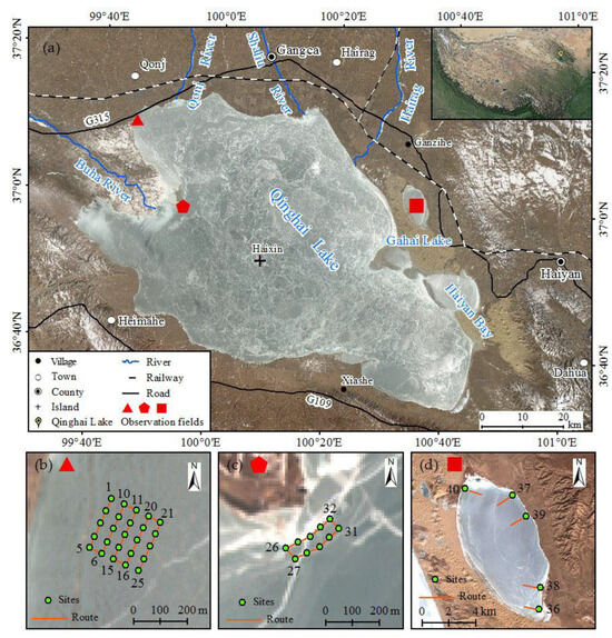
Figure 1.
Overview of the study area (a); observation field sampling sites and UAV routes (b–d).
3. Materials and Methods
3.1. Radar Principle of Ice Thickness Measurement
According to the principle of radar wave propagation, the propagation velocities of radar waves in different media are related to the dielectric constant. The dielectric constants of air, ice, water, and sandstone (slit) are 1, 3–4, 80, and 5–40, respectively. Therefore, there are differences in the propagation velocities of radar waves in different media, and the received signals can reflect the positions of these different media [30]. A radar wave enters two different types of media at different speeds, which causes not only the amplitude of the reflection coefficient R to change, but also the polarity (positive and negative) to change in relation to the characteristics of the reflection source waveform [24]. The reflection coefficient R of the radar wave can be calculated using Equation (1):
where R is the reflection coefficient, and ε1 and ε2 are the dielectric constant of two different media. According to Equation (1), the greater the difference between the dielectric constants of the two media, the larger the absolute value of the reflection coefficient. The positive- and negative-phase polarities change in response to a significant change in dielectric constant, which occurs when the radar wave propagates through the interfaces of different media. Therefore, the locations of the different interfaces can be determined by the change in phase polarity of the radar wave image.
As shown in Figure 2, we have only used a drone with a radar. The radar emits high-frequency radar waves, and when it reaches the air–ice interface and the ice–water interface, areflection occurs. The drone was flown at a constant speed, and the reflected radar wave signals were received by the antenna. We assumed that the radar waves took the same amount of time in transmitting to the interfaces and returning to and being received by the antenna, so the two-way travel time through the media can be calculated using Equation (2):
where t is the two-way travel time of radar waves, H is the ice thickness, v is the propagation velocity of the radar wave in ice, and d is the distance between the transmitting antenna and the receiving antenna, i.e., it is the distance moved by the drone in time t.
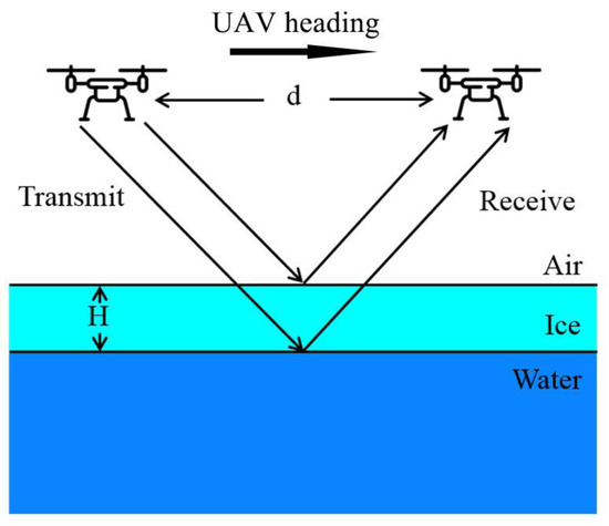
Figure 2.
Working principle of the radar ice thickness measurement.
According to the radar theory, the propagation velocity of radar waves in a specific media can be expressed as:
where v represents the propagation velocity of the radar waves in the medium (m/ns), c denotes the propagation velocity of radar waves in a vacuum (0.3 m/ns), and ε denotes the ice layer’s real complex dielectric constant.
Then, the thickness of the measured media (H) can be obtained using Equation (4):
when performing in situ measurements, the value of d is small relative to H, and can be ignored, so the equation can be simplified as follows:
Since the velocity of radar wave propagation in ice is influenced by the dielectric constant, the key to determining the thickness of ice is to determine the equivalent dielectric constant. When the in situ thickness of the ice and the radar wave propagation time are known, the equivalent dielectric constant can be deduced.
3.2. Radar Equipment
We used an IGPR (ice- and ground-penetrating radar) system (IGPR-30, Dalian Zoroy Scientific Instrument Co., Ltd., Dalian, China) to measure ice thickness. The ice detection accuracy reached the mm level, and the maximum detection depth was 6 m. Four modes of sampling points were available: 526, 512, 1024 and 2048, and 1024 was selected for sampling. The minimum time window was 2 ps, and the radar dynamic range was greater than 120 dB. The radar was connected to a GPS antenna, while the latitude and longitude coordinates were positioned with cm-level accuracy, and the UAV was equipped with a 200 W pixel camera to record video. The radar was powered with lithium batteries, and its working ambient temperature was between −30 °C and +60 °C. A GPR with a center frequency of 400 MHz was used for the January 2019 experiment, and one with a frequency of 900 MHz was used in January 2021. Both frequencies of GPR are able to meet the depth range requirements of lake ice detection.
The radar was carried on a multi-rotor UAV platform (Matrice 600 Pro, Shenzhen DJI Innovation Technology Co., Ltd., Shenzhen, China), as shown in Figure 3. The UAV had a maximum payload of 6 kg, meaning it could carry the weight of the radar module (5 kg). During the airborne measurements, the maximum flight altitude was 20 m, the maximum range of each flight was 5 km, and the maximum remote controlling distance was 2 km.
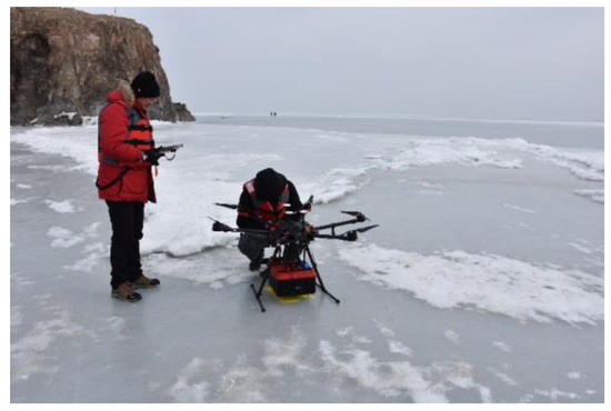
Figure 3.
UAV-borne ice-penetrating radar system, DJI Matrice 600 Pro with a radar.
3.3. Data Acquisition
Two observation fields were set up on the western shore of Qinghai Lake in January 2019, as shown in Figure 4a (an overhead image of Bird Island). We used manual drilling and airborne radar measurements to determine the ice thickness. Sample sites were placed in the observation fields at equal intervals of 50 m. The locations of the sample sites were marked with yellow tape stickers. We then used the DJI GS Pro 2.0 software for route planning based on the locations of the sample sites. To reduce radar signal attenuation along the flight path and ensure the attitude stability of the UAV, we set the altitude to 2 m and the flight speed to 2 m/s, and a wind speed of force 5 or less was assumed when flying (Figure 4b). Markers were placed at predetermined borehole locations prior to acquiring radar data. When the UAV was operating, videos were acquired using a camera mounted on the side of the radar. During data processing, the radar waves were compared with the video to obtain instantaneous radar images of the marker. The airborne device emitted radar waves continuously during the flight, meeting the detection requirements of a single site or continuously changing positions. We immediately drilled holes at the sample sites after the aerial measurements to ensure temporal and spatial consistency in the radar ice thickness measurements and the drilled ice thickness measurements (Figure 4c). After drilling, we measured the thickness of the lake ice using an electronic caliper (Figure 4d). In total, 35 holes (P1~P35) were drilled after the radar data acquisition and were used for verifying the interpretation of the radar profiles. Using the same methodology, we obtained ice thickness data from a further 5 boreholes (P36~P40) and UAV-borne radar measurements for Gahai Lake in January 2021.
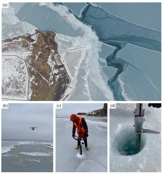
Figure 4.
Photos of the field experiment site (a). UAV-borne radar measurements of the thickness of the lake ice (b); and drill hole (c); using electronic calipers to measure lake ice thickness (d).
3.4. Radar Data Pre-Processing
The raw radar data were processed using GPR studio 2.0 software. To develop better machine understanding of the targeted characteristics, four processes were completed: zero-offset removal, bandpass filtering, amplitude gain, and layer tracking, respectively. Zero-offset refers to the unavoidable occurrence of low-frequency noise in each radar trace, predominantly arising from inductive coupling effects or electronic saturation along the ground–air interface [31,32]. This produces a zero-offset signal, which affects the subsequent process because the low-frequency component blocks the true signal after the amplitude gain. Subtracting the mean signal amplitude is a practical approach to eliminating the zero-offset phenomenon [33].
where x′(t) is the original signal trace, x*(t) denotes the signal after zero-offset removal, and ti (i = 1, 2, …, n) represents the sampling time. Figure 5 shows a comparison between before and after zero-offset removal.
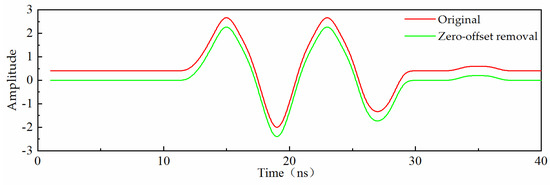
Figure 5.
Changes in GPR trace before and after zero-offset removal.
The bandpass filtering is in the frequency range from 200 to 2000 MHz, and the window function uses the Hamming. During the propagation of radar waves, energy decays with time due to dielectric losses and geometric spreading consumption (strong scattering and refraction) [34]. Considering the above issues of attenuation, an amplitude gain in radar echoes is required, which is a necessary process when seeking to amplify the return signal to a distinguishable level, and can be achieved by combining the exponential and linear functions. In Figure 6a, an original image of the radar data is shown. Figure 6b shows the image after zero-drift removal and bandpass filtering, and Figure 6c shows the radar echo after the amplitude gain.
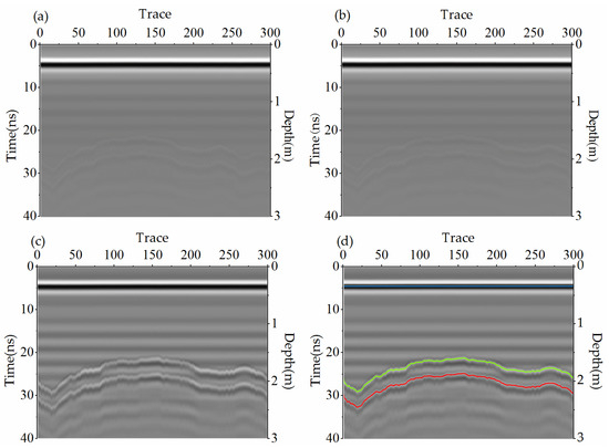
Figure 6.
GPR echoes pre-processing. Raw data (a); data after zero-offset removal and bandpass filtering (b); amplitude gain (c); data after layer tracking (d). The green line represents the interface between air and ice, the red line represents the interface between ice and water, and the blue line indicates the height of the UAV.
Images of thickness measured by the radar typically take the form of pulse waves. The positive and negative peaks of the waveform are represented, respectively, in black and white, or in gray scale and color. In this way, the interfaces of different media and their fluctuations can be clearly inferred from the in-phase axis or equal gray scale and equal color line [24]. As shown in Figure 6c, the first interface encountered by the radar wave during propagation is the air–ice interface, where the color change in the in-phase axis is black–white–black and the corresponding change in polarity is + - +, indicating that the radar wave has reached a medium with a higher dielectric constant than that of the original (ε air < ε ice). The second interface is the ice–water interface, where the color change in the in-phase axis is also black–white–black, and the polarity change is also + - +, indicating that the radar wave reaches a medium with a higher dielectric constant than ice (ε ice < ε water). After the above pre-processing of the radar echoes, the air–ice and ice–water interfaces can be clearly identified in the radar echo images, thus allowing us to determine the time taken for the radar waves to propagate through the ice and calculate the ice thickness from the time. We determined the locations of the drilled holes by examining the images taken during drone flight while hovering and flying, corresponding to the range of radar echo image channels in order to calculate the simulated thickness at the drilled hole locations. Figure 6d shows the results of layer tracking with pre-processed radar echoes.
3.5. Extraction of Amplitudes
In order to obtain the characteristics of radar wave variations at different interfaces, a script program was written to extract the amplitudes from all radar data, and the amplitude variations in the characteristic regions were plotted according to the locations of the sampling sites and the radar wave traces.
3.6. Accuracy Validation
In order to quantify the accuracy of our airborne radar measurements of lake ice thickness, root mean square error (RMSE) and percentage error were used, as follows:
where H0 is the in situ thickness, H is the radar thickness, λ is the percentage error, and n represents the number of sampling sites.
4. Results
4.1. Radar Echo Profiles
Reflections in the radar profiles were used to calculate the ice thickness [35]. In the radar profiles taken from both observation fields, reflections at each interface are evident and can be easily traced. In situ data acquisition from the drilled holes confirmed that the ice–water interfaces yielded lower reflections. Reflections in the radar profiles also originate from other factors besides air–ice and ice–water interfaces. In Figure 7a, the waveforms in regions A1 and A2 reflect the UAV taking off and landing, respectively. In Figure 7b, the waveforms in regions B1 and B3 indicate the presence of cracks in the ice surface and the upward surface distortion of the radar waveform, while the waveforms in regions B2 and B4 indicate a buildup of ice and an abrupt downward distortion of the radar waveform. Figure 7c shows the radar profiles of the ground–ice interface, e.g., the waveforms in region C1 indicate that the ice was touching the ground. The waveforms at C2 indicate the presence of other objects on the surface of the ice—in this case mostly bare rock. In addition, we also obtained radar waveforms without a stable freeze forming. In Figure 7d, which shows the unfrozen lake, only one interface has been captured in the radar waveform showing the formation of an ice–water mixture, rather than two.
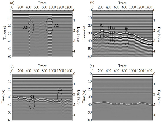
Figure 7.
The UAV-borne ice-penetrating radar echo profiles’ interpretation. The radar profiles during take-off and landing (a); the radar profiles of the ice surface in the presence of cracks and ice build-up (b); the radar profiles of the ground-ice interface (c); the radar profiles of ice-water mixtures (d).
4.2. Amplitude Variation of Radar
We identified the positions of the sampling sites from the aerial flight videos of the UAV, and extracted the two-way travel times and echo images for the radar waves at each sampling site. Figure 8a,b shows the radar echoes of 35 sampling sites in two observation fields. The color of the in-phase axis in the figure reflects polarity change in the radar wave, i.e., the amplitude change in the radar wave. The Y-axis indicates the propagation time of the radar wave; the time taken for the radar wave to reach the upper interface of the ice layer (air–ice) was 23.51~34.24 ns, and the time to reach the lower interface of the ice layer (ice–water) was 27.50~40.72 ns. The two-way travel time in the ice was 3.79 ns. At the same time, the amplitudes of the radar wave at the upper and lower ice interfaces at each sampling sites were extracted based on the arrival time at each sampling point, and then the amplitudes were divided by the maximum value in the measurement area to obtain the normalized amplitude. The normalized amplitudes of the radar waves at the upper and lower ice interfaces at all sampling points are shown in Figure 8c,d. These may be related to variations in the water content of the ice at different depths. The increase in the water content from the surface to the bottom of the ice leads to the enhanced absorption of radar waves by the medium, resulting in a gradual decrease in radar wave amplitude. It is of interest that the bedding surface at the location of borehole P32 is a lakebed deposit (bedrock) with a significantly lower normalized amplitude value (0.07) than the average amplitude of the ice floes at other locations (0.48).
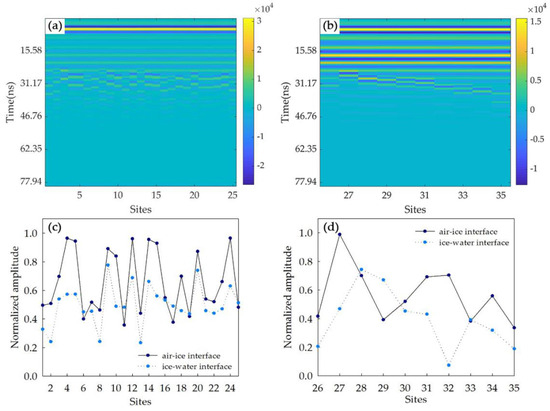
Figure 8.
Interpretation of the UAV-borne ice-penetrating radar profile in Qinghai Lake. The radar echoes of 35 sampling sites in two observation fields (a,b); the normalized amplitudes of the radar waves at the upper and lower ice interfaces at all sampling points (c,d).
4.3. Accuracy Validation and Observation Fields’ Ice Thickness
The propagation velocity of radar waves in ice can be calculated using the in situ ice thickness and the propagation time. In Figure 9, the indicators are shown for sampling sites at Qinghai Lake (P1~P35) and Gahai Lake (P36~P40). The trends of in situ ice thickness and radar wave propagation time show that the propagation time decreased as ice thickness decreased, which indicates that the radar wave propagation velocity in the ice remained between 0.121 m/ns and 0.180 m/ns. The mean velocity at the Qinghai Lake observation point was 0.146 m/ns and that at Gahai Lake was 0.140 m/ns, which are both below the standard velocity of radar waves in ice.
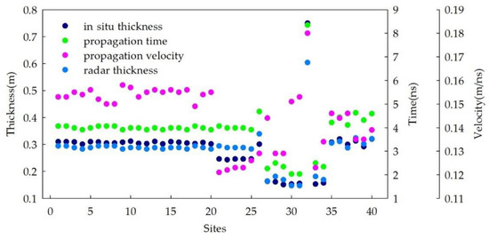
Figure 9.
Observed in situ ice thickness, propagation time, propagation velocity, and radar thickness.
The calculations of dielectric constant show that the mean value at the Qinghai Lake observation site was 4.3, and the mean at Gahai Lake was 4.6. In calculating the ice thickness from the respective mean values, the measurements using a 400 MHz radar at Qinghai Lake were lower than those taken in situ at 24 of the 35 points, and ice thickness was overestimated at the remaining points. Based on Equations (7) and (8), the RMSE was 0.034 m, and percentage error of was 8.6%. The results for Gahai Lake taken using 900 MHz radar showed an RMSE of 0.010 m, with a percentage error of 2.8%.
Figure 10a,b shows the continuous variation in ice thickness at the Lake Qinghai observation fields 1 and 2, respectively, with some variation seen in the characteristics of lake ice thickness. The radar-measured ice thickness in field 1 ranged from 0.276 to about 0.299 m, and the mean ice thickness was 0.287 m, with a small variation. The radar-measured ice thickness at field 2 ranged from 0.141 to about 0.648 m, with a mean ice thickness of 0.198 m and a wide range of variations.
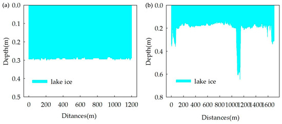
Figure 10.
Radar-measured ice thickness at Qinghai Lake observation fields 1 (a) and 2 (b).
5. Discussion
When utilizing a radar to calculate ice thickness, it is crucial to accurately determine the velocity of radar wave propagation through the ice. The results of this study for radar wave propagation velocity differ from those of previous studies. In a slight departure from other scholarly studies on sea ice [16,17], river ice [18,20,30], glacial ice [21,24,36], lake ice [26], and reservoir ice [28], our experiments yielded lower mean velocities and higher dielectric constants than freshwater ice. Experiments by Zhang [30] undertaken on the Yellow River showed that radar waves propagate at a velocity of 0.163 m/ns during peak ice and at less than 0.150 m/ns during melting. This illustrates that differences in the moisture content on the ice surface or in the ice affect the velocity of radar wave propagation. Therefore, regarding the annual lake ice of Qinghai Lake and Gahai Lake, the moisture content is generally high, causing the radar wave propagation velocity to be low. In addition, considering that Qinghai Lake is a brackish lake located on the Qinghai–Tibet Plateau, the higher salinity of the water causes its freezing point to be lower than that of freshwater ice bodies, and temperature changes in the ice in turn affect the dielectric constant of the ice. In contrast, although Qinghai Lake and Gahai are in the same area, the propagation characteristics of radar waves through the ice on the two lakes are somewhat affected by differences in their salinity. Salt and brine lakes are also present on the Qinghai–Tibet Plateau [37], and their salinity affects the freezing of lake water, while the dielectric constants of these lakes’ ice differ from those of freshwater ice.
Air bubbles in the ice can increase the velocity of radar wave propagation, and thus affect the accuracy of ice thickness calculations [35]. When the rate of proportion of air bubbles in the ice is high, the velocity of the radar waves can reach 0.21 m/ns [38], which would result in a large error if the standard velocity of radar waves in ice (0.17 m/ns) were to be used [39,40]. Li [28] showed that radar waves propagate at a speed of 17.02 m/ns in granular ice and 16.98 in columnar ice. This implies that differences in ice structure and air bubble content affect the propagation characteristics of radar waves in ice. Due to the bubbles in the ice, the GPR waves are scattered and the average velocity increases with the bubble volume ratio; the velocity increases by 0.0014 m/ns for every 1% increase in bubble volume [35]. Ice thickens via the congelation of ice at the water and ice interface. Congealed ice contains elongated bubbles, which are trapped within the ice, and cause radar waves to be scattered and reflected back [41]. In general, the low bubble contents in lake ice on the Tibetan Plateau and the unfrozen water in the ice counteract the increase in radar wave velocity in the ice, meaning that the ice thickness can be calculated with high accuracy [35]. According to field observations, the ice on Qinghai Lake and Gahai Lake during the freeze-up period is columnar. This is because, when the lake water was frozen, salt was entrained in the ice in salt cells, and over time, brine channels formed between the ice, and the residual high concentration of salt was discharged along the channels. The bubble contents of brine channels in the ice are low, meaning that they have a reduced effect on the radar wave propagation velocity. Since the dielectric constant of ice is related to its crystal structure and temperature, it is necessary to determine the in situ thickness of ice using boreholes during each probing, invert the effective dielectric constant of the ice layer based on in situ ice thickness, and then simulate and calculate the final ice thickness based on this value [30].
The type of lake ice also affects the amplitude of the radar waves. In this experiment, the drilling results show that the majority of the measurement area comprised floating ice. Due to the great difference between the dielectric constants of ice and water, the reflection energy of the ice–water interface is strong, and the amplitude of reflection of radar waves by floating ice is significantly stronger than that of grounded ice—about 3~4 times the average reflection amplitude [17,20,42]. The average reflection amplitude of the floating ice in the experiment was seven times greater than that of touchdown ice, which is higher than values derived in previous studies.
In addition to the propagation velocity within the ice, the accuracy of ice thickness measurements is also related to the frequency of the antenna. The frequency of the transmitting antenna determines the detection depth, while the frequency of the receiving antenna has an effect on the resolution [43]. High-frequency signals in low-velocity media are characterized by short wavelengths and a high resolution, while low-frequency signals in high-velocity media have a low resolution. The attenuation of radar signals is significantly affected by the antenna frequency, with higher frequencies being more significantly attenuated than lower frequencies. This frequency attenuation behavior therefore explains the greater penetration of radar signals at lower frequencies than at higher frequencies [44]. In general, longer waves penetrate deeper into the medium, while shorter waves provide a higher resolution. Once the approximate depth of the target is known, it is recommended to select a higher-frequency antenna capable of penetrating to that depth in order to secure the required resolution and penetration depth. In the experiments in this paper, we used 400 and 900 MHz antennae. During data processing, it was found that the images acquired by the 900 MHz frequency radar had a higher resolution and captured data from the interface more accurately compared to 400 MHz, and the results of ice thickness measurements show that the 900 MHz radar also had better accuracy.
Arbitrary underground medium inhomogeneity and undesired measurement noises often disturb radar data interpretation [45]. A lake with a more homogeneous subsurface, such as Qinghai Lake, has a flatter ice surface, and this ensures better data collection when it enters the stable freeze-up period in winter. However, in the initial freezing period when the ice is thin, or when an ice–water mixture is formed on the lake surface, it is more difficult to distinguish the upper and lower ice interfaces in the radar image; only the air–lake interface can be easily identified. In addition, working with UAV-borne ice-penetrating radar requires control of the UAV’s altitude. We found that when the UAV returned at an altitude of 20 m, ice information was not recognized, even though the radar data had been pre-processed. Therefore, it is advisable to keep UAV flights to a height of less than 10 m.
In conclusion, excluding the above factors that affect the propagation characteristics of radar waves in ice. In order to secure the accuracy of the experimental data, we should obtain the in situ thickness and the propagation time of the radar wave as accurately as possible. Since the velocity of radar wave propagation in ice is affected by the dielectric constant, the critical factor in determining the ice thickness using airborne ice-penetrating radar is to determine the equivalent dielectric constant. As shown in Equation (5), since the propagation velocity of radar waves in air is known, the equivalent dielectric constant can be derived when the in-situ thickness of the ice and the propagation time of the radar waves are obtained. This is the rationale for using two different equivalent dielectric constants for Qinghai Lake and Gahai Lake, two lakes with differences in salinity, temperature, and other properties of the water. When modeling ice thickness using this equipment, it is important to accurately obtain the in situ ice thickness and radar wave propagation time in order to calculate a more accurate equivalent dielectric constant with as many measured points as possible.
6. Conclusions
In this study, UAV-borne ice-penetrating radar was used to detect the ice thickness of Qinghai Lake and Gahai Lake, and the ice thickness at in situ boreholes was used to verify the radar measurements. The echo pattern characteristics of the airborne radar and the propagation characteristics of the radar waves in the lake ice were clarified. The applicability of a UAV-borne ice-penetrating radar for ice thickness detection in winter glacial lakes was explored. The main conclusions are as follows:
- After pre-processing the echo images obtained with the UAV ice-penetrating radar, we were able to clearly assess the lake ice developing during the stable freezing period and accurately determine the propagation times of the radar waves through the ice.
- Contrasting our in situ measurements of ice thickness, the mean velocity of radar wave propagation in the ice was lower than that in other regions, and the dielectric constant was higher. Compared with in situ ice thickness measurements for Qinghai Lake, measurements taken using a 400 MHz radar showed an RMSE of 0.034 m with a percentage error of 8.6%, while the results for Gahai using a 900 MHz radar showed an RMSE of 0.010 m with a percentage error of 2.8%.
- The use of a radar with a higher antenna frequency ensures higher detection accuracy, provided that the detection depth is met. This affirms the need to control the altitude and speed of the UAV during airborne ice-penetrating radar thickness measurements.
In future lake ice surveys, the use of UAVs with an ice-penetrating radar will help quickly obtain accurate information on ice thickness. However, in the alpine region, conditions are vicious, with low temperatures, thin air, and other problems, and the life of a UAV’s single battery is short, meaning that it is easy to lose altitude when flying continuously. These difficulties will need to be overcome in the future in order to complete a large number of lake ice surveys using an airborne radar.
Author Contributions
Conceptualization, H.J. and X.Y.; Methodology, H.J. and X.Y.; software, H.J., S.Z., Y.Z. and J.C.; formal analysis, X.Y.; investigation, H.J., X.Y., Q.W., S.Z. and Y.Z.; instrumentation support, J.C. and Z.Y.; data analysis, H.J., X.Y., Q.W. and Z.Y.; writing—original draft preparation, H.J.; writing—review and editing, H.J., X.Y. and Q.W.; visualization, H.J.; supervision, X.Y.; project administration, X.Y.; funding acquisition, X.Y. All authors have read and agreed to the published version of the manuscript.
Funding
The National Natural Science Foundation of China (41861013, 41801052, 42071089); Wetland Protection and Restoration Project under the Second Batch of Central Finance Forestry Reform and Development Wetland Subsidy Fund in 2022 (QHDY2022-12-12A); Gansu Province University Innovation Fund Project in 2022 (2022A-256) and Chinese Academy of Sciences “Light of West China” Program.
Data Availability Statement
Data are contained within the article.
Acknowledgments
We would like to thank our colleagues at Northwestern Normal University for their help with the writing process. We would like to thank those who helped us in the experiment. We thank the anonymous reviewers and editors for their constructive suggestions.
Conflicts of Interest
The authors declare no conflicts of interest. Ji Chen is employed by Dalian Zhongrui Science and Technology Development Co., Ltd. The funders had no role in the design of the study; in the collection, analyses, or interpretation of data; in the writing of the manuscript; or in the decision to publish the results.
References
- Wetzel, R.G. Lake and River Ecosystems. Nature 2001, 21, 1–9. [Google Scholar]
- Magnuson, J.J.; Benson, B.J.; Kratz, T.K. Temporal coherence in the limnology of a suite of lakes in Wisconsin, USA. Freshw. Biol. 1990, 23, 145–159. [Google Scholar] [CrossRef]
- Du, J.Y.; Kimball, J.S.; Duguay, C.; Kim, Y.; Watts, J.D. Satellite microwave assessment of Northern Hemisphere lake ice phenology from 2002 to 2015. Cryosphere 2017, 11, 47–63. [Google Scholar] [CrossRef]
- Sharma, S.; Meyer, M.F.; Culpepper, J.; Yang, X.; Hampton, S.; Berger, S.A.; Brousil, M.R.; Fradkin, S.C.; Higgins, S.N.; Jankowski, K.J.; et al. Integrating Perspectives to Understand Lake Ice Dynamics in a Changing World. J. Geophys. Res. 2020, 125, e2020JG005799. [Google Scholar] [CrossRef]
- Sharma, S.; Blagrave, K.; Magnuson, J.J.; O’Reilly, C.M.; Oliver, S.; Batt, R.D.; Magee, M.R.; Straile, D.; Weyhenmeyer, G.A.; Winslow, L. Widespread loss of lake ice around the northern hemisphere in a warming world. Nat. Clim. Change 2019, 9, 227–231. [Google Scholar] [CrossRef]
- Guo, L.N.; Wu, Y.H.; Zheng, H.X.; Zhang, B.; Li, J.S.; Zhang, F.F.; Shen, Q. Uncertainty and variation of remotely sensed lake ice phenology across the tibetan plateau. Remote Sens. 2018, 10, 1534. [Google Scholar] [CrossRef]
- Yang, X.; Pavelsky, T.M.; Allen, G.H. The past and future of global river ice. Nature 2020, 577, 69–73. [Google Scholar] [CrossRef]
- Kouraev, A.V.; Semovski, S.V.; Shimaraev, M.N.; Mognard, N.M.; Légresy, B.; Remy, F. Observations of Lake Baikal ice from satellite altimetry and radiometry. Remote Sens. Environ. 2007, 108, 240–253. [Google Scholar] [CrossRef]
- Qin, D.H.; Dong, W.J.; Luo, Y. Climate and Environment Changes in China: 2012 Volume I Scientific Basis; China Meteorological Press: Beijing, China, 2012. [Google Scholar]
- Fu, H.; Liu, Z.P.; Guo, X.L.; Cui, H.T. Double-frequency ground penetrating radar for measurement of ice thickness and water depth in rivers and canals: Development, verification and application. Cold Reg. Sci. Technol. 2018, 154, 85–94. [Google Scholar] [CrossRef]
- Worby, A.P.; Griffin, P.W.; Lytle, V.I.; Massom, R.A. On the use of electromagnetic induction sounding to determine winter and spring sea ice thickness in the Antarctic. Cold Reg. Sci. Technol. 1999, 29, 49–58. [Google Scholar] [CrossRef]
- Brown, L.C.; Duguay, C.R. A comparison of simulated and measured lake ice thickness using a Shallow Water Ice Profiler. Hydrol. Process 2011, 25, 2932–2941. [Google Scholar] [CrossRef]
- Hawley, N.; Beletsky, D.; Wang, J. Ice thickness measurements in Lake Erie during the winter of 2010–2011. J. Great Lakers Res. 2018, 44, 388–397. [Google Scholar] [CrossRef]
- Ghobrial, T.R.; Loewen, M.R.; Hicks, F.E. Continuous monitoring of river surface ice during freeze-up using upward looking sonar. Cold Reg. Sci. Technol. 2013, 86, 69–85. [Google Scholar] [CrossRef]
- Beckers, J.F.; Casey, J.A.; Haas, C. Retrievals of Lake Ice Thickness From Great Slave Lake and Great Bear Lake Using CryoSat-2. IEEE Trans. Geosci. Remote Sens. 2017, 55, 3708–3720. [Google Scholar] [CrossRef]
- Holt, B.; Kanagaratnam, P.; Gogineni, S.P.; Ramasami, V.C.; Mahoney, A.; Lytle, V. Sea ice thickness measurements by ultrawideband penetrating radar: First results. Cold Reg. Sci. Technol. 2009, 55, 33–46. [Google Scholar] [CrossRef]
- Stevens, C.W.; Moorman, B.J.; Solomon, S.M.; Hugenholtz, C.H. Mapping subsurface conditions within the near-shore zone of an Arctic delta using ground penetrating radar. Cold Reg. Sci. Technol. 2009, 56, 30–38. [Google Scholar] [CrossRef]
- Galley, R.J.; Trachtenberg, M.; Langlois, A.; Barber, D.G.; Shafai, L. Observations of geophysical and dielectric properties and ground penetrating radar signatures for discrimination of snow, sea ice and freshwater ice thickness. Cold Reg. Sci. Technol. 2009, 57, 29–38. [Google Scholar] [CrossRef]
- Arcone, S.A.; Delaney, A.J. Airborne River-ice Thickness Profiling with Helicopter-borne UHF Short-pulse Radar. J. Glaciol. 1987, 33, 330–340. [Google Scholar] [CrossRef]
- Kämäri, M.; Alho, P.; Colpaert, A.; Lotsari, E. Spatial variation of river-ice thickness in a meandering river. Cold Reg. Sci. Technol. 2017, 137, 17–29. [Google Scholar] [CrossRef]
- Wang, B.B.; Tian, G.; Cui, X.B.; Zhang, X.P. The internal COF features in Dome A of Antarctica revealed by multi-polarization-plane RES. Appl. Geophys. 2008, 5, 230–237. [Google Scholar] [CrossRef]
- Welch, B.C.; Jacobel, R.W.; Arcone, S.A. First results from radar profiles collected along the US-ITASE traverse from Taylor Dome to South Pole (2006–2008). Ann. Glaciol. 2009, 50, 35–41. [Google Scholar] [CrossRef][Green Version]
- Barzycka, B.; Błaszczyk, M.; Grabiec, M.; Jania, J. Glacier facies of Vestfonna (Svalbard) based on SAR images and GPR measurements. Remote Sens. Environ. 2019, 221, 373–385. [Google Scholar] [CrossRef]
- Liu, J.; Wang, S.; He, Y.; Li, Y.; Wang, Y.; Wei, Y.; Che, Y. Estimation of ice thickness and the features of subglacial media detected by ground penetrating radar at the Baishui River Glacier No. 1 in Mt. Yulong, China. Remote Sens. 2020, 12, 4105. [Google Scholar] [CrossRef]
- Proskin, S.A.; Parry, N.S.; Finlay, P. Applying GPR in Assessing the Ice Bridges, Ice Roads and Ice Platforms. In Proceedings of the CGU HS Committee on River Ice Processes and the Environment, Winnipeg, MB, Canada, 16 September 2011. [Google Scholar]
- Gusmeroli, A.; Grosse, G. Ground penetrating radar detection of subsnow slush on ice-covered lakes in interior Alaska. Cryosphere 2012, 6, 1435–1443. [Google Scholar] [CrossRef]
- Gunn, G.E.; Duguay, C.R.; Brown, L.C.; King, J.; Atwood, D.; Kasurak, A. Freshwater lake ice thickness derived using surface-based X-and Ku-band FMCW scatterometers. Cold Reg. Sci. Technol. 2015, 120, 115–126. [Google Scholar] [CrossRef]
- Li, Z.J.; Qing, J.; Zhang, B.S.; Leppäranta, M.; Lu, P.; Huang, W.F. Influences of gas bubble and ice density on ice thickness measurement by GPR. Appl. Geophys. 2010, 7, 105–113. [Google Scholar] [CrossRef]
- Qi, M.M.; Yao, X.J.; Li, X.F.; An, L.N.; Gong, P.; Gao, Y.P.; Liu, J. Spatial-temporal characteristics of ice phenology of inghai Lake from 2000 to 2016. J. Geogr. Sci. 2018, 73, 932–944. [Google Scholar]
- Zhang, B.S.; Zhang, F.X.; Liu, Z.Y.; Han, H.W.; Li, Z.J. Field Experimental Study of the Characteristics of GPR Images of Yellow River ice. South-to-north water trans. Chin. J. Water Sci. Technol. 2017, 15, 121–125. [Google Scholar]
- Cassidy, N.J. Ground Penetrating Radar Data Processing, Modelling and Analysis. In Ground Penetrating Radar: Theory and Applications; Jol, H.M., Ed.; Elsevier: Oxford, UK, 2008; pp. 141–176. [Google Scholar]
- Shamir, O.; Goldshleger, N.; Basson, U.; Reshef, M. Laboratory measurements of subsurface spatial moisture content by ground-penetrating radar (GPR) diffraction and reflection imaging of agricultural soils. Remote Sens. 2018, 10, 1667. [Google Scholar] [CrossRef]
- Jin, Y.; Duan, Y. Wavelet Scattering Network-Based Machine Learning for Ground Penetrating Radar Imaging: Application in Pipeline Identification. Remote Sens. 2020, 12, 3655. [Google Scholar] [CrossRef]
- Jin, Y.; Duan, Y. A new method for abnormal underground rocks identification using ground penetrating radar. Measurement 2020, 149, 106988. [Google Scholar] [CrossRef]
- You, Y.H.; Yang, M.B.; Yu, Q.H.; Pan, X.C.; Guo, L.; Wang, X.B.; Wu, Q.B. Factors influencing the reliability of grounded and floating ice distinguishing based on ground penetrating radar reflection amplitude. Cold Reg. Sci. Technol. 2018, 154, 1–8. [Google Scholar] [CrossRef]
- Sun, B.; He, M.; Zhang, P.; Jiao, K.; Wen, J.; Li, Y. Determination of ice thickness, subice topography and ice volume at Glacier No.1 in the Tianshan, China, by ground penetrating radar. Chin. J. Polar Sci. 2003, 15, 35–44. [Google Scholar]
- Niu, F.; Lin, Z.; Liu, H.; Lu, J. Characteristics of thermokarst lakes and their influence on permafrost in Qinghai-Tibet plateau. Geomorphology 2011, 132, 222–233. [Google Scholar] [CrossRef]
- Finlay, P.I.; Parry, N.S.; Proskin, S.A.; Mickle, R.J. An overview of ice profiling using ground penetrating radar (GPR). In Proceedings of the 21st EEGS Symposium on the Application of Geophysics to EngIneering & Environmental Problems, Philadelphia, PA, USA, 6 April 2008. [Google Scholar]
- Annan, A.P.; Diamanti, N.; Redman, J.D.; Jackson, S.R. Ground-penetrating radar for assessing winter roads. Geophysics 2015, 81, 101–109. [Google Scholar] [CrossRef]
- Davis, J.L.; Annan, A.P. Ground-penetrating radar for high-resolution mapping of soil and rock stratigraphy. Geophys. Prospect. 1989, 37, 531–551. [Google Scholar] [CrossRef]
- Morris, K.; Jeffries, M.O.; Weeks, W.F. Ice processes and growth history on Arctic and sub-Arctic lakes using ERS-1 SAR data. Polar Record. 1995, 31, 115–128. [Google Scholar] [CrossRef]
- Jones, B.M.; Gusmeroli, A.; Arp, C.D.; Strozzi, T.; Grosse, G.; Gaglioti, B.V.; Whitman, M.S. Classification of freshwater ice conditions on the Alaskan Arctic coastal plain using ground penetrating radar and TerraSAR-X satellite data. Int. J. Remote Sens. 2013, 34, 8267–8279. [Google Scholar] [CrossRef]
- Shaikh, S.A.; Tian, G.; Shi, Z.J.; Zhao, W.K.; Junejo, S.A. Frequency band adjustment match filtering based on variable frequency GPR antennas pairing scheme for shallow subsurface investigations. J. Appl. Geophys. 2018, 149, 42–51. [Google Scholar] [CrossRef]
- Alani, A.M.; Tosti, F. GPR applications in structural detailing of a major tunnel using different frequency antenna systems. Constr. Build. Mater. 2018, 158, 1111–1122. [Google Scholar] [CrossRef]
- Kang, M.S.; An, Y.K. Frequency–Wavenumber Analysis of Deep Learning-based Super Resolution 3D GPR Images. Remote. Sen. 2020, 12, 3056. [Google Scholar] [CrossRef]
Disclaimer/Publisher’s Note: The statements, opinions and data contained in all publications are solely those of the individual author(s) and contributor(s) and not of MDPI and/or the editor(s). MDPI and/or the editor(s) disclaim responsibility for any injury to people or property resulting from any ideas, methods, instructions or products referred to in the content. |
© 2024 by the authors. Licensee MDPI, Basel, Switzerland. This article is an open access article distributed under the terms and conditions of the Creative Commons Attribution (CC BY) license (https://creativecommons.org/licenses/by/4.0/).