Abstract
Our study addresses the need for universal monitoring solutions given the diverse environmental impacts of surface mining operations. We present a solution combining remote sensing and machine learning techniques, utilizing a dataset of over 2000 satellite images annotated with ten distinct labels indicating mining area components. We tested various approaches to develop comprehensive yet universal machine learning models for mining area segmentation. This involved considering different types of mines, raw materials, and geographical locations. We evaluated multiple satellite data set combinations to determine optimal outcomes. The results suggest that radar and multispectral data fusion did not significantly improve the models’ performance, and the addition of further channels led to the degradation of the metrics. Despite variations in mine type or extracted material, the models’ effectiveness remained within an Intersection over Union value range of 0.65–0.75. Further, in this research, we conducted a detailed visual analysis of the models’ outcomes to identify areas requiring additional attention, contributing to the discourse on effective mining area monitoring and management methodologies. The visual examination of models’ outputs provides insights for future model enhancement and highlights unique segmentation challenges within mining areas.
1. Introduction
1.1. Background of the Research
The mining industry plays a significant role in supplying mineral resources for energy transition efforts [1]. The rising challenge is therefore to mine natural resources in a sustainable manner. High-tech and modern artificial intelligence methods can help to achieve this goal [2]. Mining is one of the major industrial activities that lead to land surface transformation. Among the two main mining methods—underground and surface—the latter has a greater impact on the environment due to the direct transformation of the surface and scale of material movement. As a result, an area is transformed at every stage of the mining cycle, from exploration, through deposit development, production, and mineral processing, up to mine closure and reclamation of the post-mining area. During these stages, activities such as pit creation, excavation, infrastructure construction, and waste rock disposal are responsible for the largest transformations of land surface [3].
Land use is one of the biggest environmental impacts of surface mining; hence, there is a high demand for precise and up-to-date information on land cover changes in mining areas [4]. Surface mining leads to land use that remains significant for a very long period, which underscores the significance of remote sensing methods for effective environmental monitoring. By combining remote sensing with machine learning, it is possible to create tools for automated, near-real-time monitoring of surface mining activities [5,6,7,8]. Thanks to the latest remote sensing techniques, it is possible to assess vast areas with low costs and high temporal frequency. It allows for land use monitoring, long-term mining plan verification, and detection of illegal mining activities, among other uses. Combining space-borne remote sensing data with other remote sensing data sources and machine learning can further improve the efficiency and effectiveness of these methods [9,10].
1.2. Challenges
In this research, we confronted significant challenges in the field of mining area detection and segmentation using machine learning.
Diversity of surface mining: The diversity of surface mining areas, each influenced by the type of extracted raw material, geological setting, type of mine, and the standards adopted within different countries, resulted in varied mining landscapes. The differentiation between sites creates a challenge for the development of worldwide universal machine learning models for mining area detection and segmentation [11].
The insufficiency of current segmentation approaches: Models previously published commonly resort to a limited number of land cover classes, which lack the requisite detail to capture the intricacies of mining environments [12]. To distinguish more details within the mining sites, the development of comprehensive segmentation approaches is necessary.
The difficulty in machine learning model optimization: The effectiveness of these models is contingent upon the types of satellite datasets employed and the specificity of the mine area. Determining the optimal combination of input data presents a complex task, indicative of a substantial challenge within the field [13].
In previous studies, authors have addressed these challenges by developing universal worldwide datasets with low levels of detail or very specific models that are limited to being useful for specific categories of mining-related issues. A good example would be a developed global-scale dataset of mining areas consisting of almost 45,000 polygons, or a developed index for the detection of coal mining areas that were found to be regionally specific [14]. Nevertheless, some authors combined remote sensing with machine learning for land cover classification of surface mining areas. Our review reveals that defining the number and type of land cover classes for classification algorithms can be very subjective. Depending on the goals pursued, researchers selected appropriate land cover classes concerning components of mining and post-mining areas or elements of the natural environment. Our literature review shows that mining areas are most often divided into two to six land cover classes, such as active mining area and reclaimed area, exploitation area, dumping area [15], open-pit, raw material processing area, dump [16], or area of active exploitation, wooded and bushy areas, rehabilitated areas, waste, water management, other [17].
Addressing the mentioned challenges, our study revolves around the development of universal and precision machine learning models for mining area segmentation, offering a potential solution to the issues identified above. For this work, we decided to define as many as 10 classes in total, including excavation, dumping ground, stockpile, infrastructure, and tiling storage facility, among others. To advance this objective, we embarked on a threefold approach. Firstly, we determined the optimal configuration of bands. We then conducted a comparative analysis of two distinct data splits. Finally, we focused on fine-tuning the hyperparameters.
The specific challenges faced by this study included the following: (1) defining several land cover classes of mining areas and creating proper datasets for models, which would be useful in multipurpose mining area segmentation tasks; (2) proposing a dataset that splits the criteria to optimize models’ performances; (3) applying machine learning models to multidimensional data; (4) training machine learning models on a very large dataset.
2. Materials and Methods
2.1. Training Data
The initial version of the machine learning dataset was created utilizing the Earth Observation (EO) data derived from Sentinel satellites’ optical and radar sensors. The Sentinel-2 (S2) MSI (Multispectral Imagery) Level-2A product was employed, containing 12 spectral bands of spatial resolution varying between 10, 20, and 60 m, along with a superficial classification layer, as depicted in Figure 1. In addition, we included Sentinel-1 (S1) high-resolution Level-1 Ground Range Detected scenes, featuring dual-band cross-polarization (vertical transmit/horizontal and vertical receive, i.e., VV + VH) and their combination (VV/(10 × VH)). The radar data values were transformed to decibels using the logarithmic scaling method (). Due to the discrepancy in spatial resolution, we resampled all S1 and S2 scenes to 10 m Ground Sample Distance (GSD) utilizing the nearest neighbor interpolation technique. The final step was merging all of them into the fused product of optical and radar data.
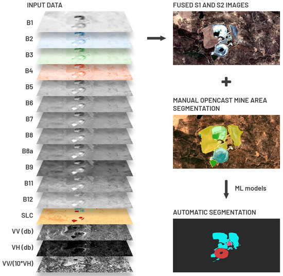
Figure 1.
A schematic diagram of the data fusion workflow in a semantic segmentation task.
We have collected and prepared an EO dataset consisting of more than 2000 images from over 400 mining areas located across 5 continents and over 40 countries (Figure 2). To improve the generalization capabilities of the dataset, we have differentiated the mining areas based on the extracted raw material (rock raw materials, metallic ores, coal and lignite), among others. We utilized multiple satellite images of each area, covering the time series from 2016 to 2022. Notably, the selection of this time range is motivated by the availability of Sentinel-2 (S2) data from 2016 onwards. For each year within this period, we selected one cloudless representative image. This allowed us to include the variability of individual mining area components over time and thereby optimize the labeling process, in addition. The main criterion for label definition was to annotate all the parts of the surface mining areas while avoiding rather unique or site-specific labels to be able to provide a sufficient number of ground truth data. The ground truth labels for the datasets were manually annotated by a group of mining engineers. These annotations were later compared and reviewed, establishing target labels for datasets. Our objective was to identify the most common and significant components of mining areas. However, due to the variability of surface mines, certain components were specific to their types, which could have posed the risk of having an insufficient number of training samples. Therefore, the annotation process required us to compromise and simplify certain definitions to avoid defining numerous cover classes while labeling almost the entire area transformed by mining. As a result of the compromises made, we removed, among others, labels such as deposit outcrop and overburden.
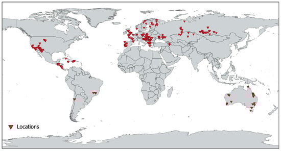
Figure 2.
Locations of mining areas used for dataset preparation.
Furthermore, we had to take into account the limitations of machine learning in object recognition. Therefore, we did not include reclaimed areas in our analysis, as the deep learning model might encounter difficulty in recognizing lakes, croplands, or forests that result from the reclamation process, rather than from other natural or anthropogenic processes.
Based on the aforementioned considerations, we selected 10 classes of mining area coverage. The assumed definitions of the defined land cover classes for this research are presented in Table 1.

Table 1.
Label descriptions (description of labels used for annotation of mining area land cover classes).
The unlabeled portions of the image were designated as background for use in machine learning model training tasks. To enhance the metrics of our ML models, we introduced a blank label to better differentiate between unaltered or reclaimed regions and transformed areas. The annotated data for the chosen satellite image are exemplified in Figure 3. Particular attention should be paid to the level of accuracy and precision of the annotation process.
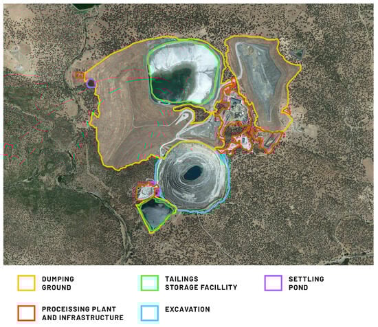
Figure 3.
Exemplary annotation of mining area land cover classes used for machine learning model training. Aquablanca Mine, Spain.
2.2. Subsets of Training Data
Components of mining areas frequently fall into multiple defined classes simultaneously. For example, both the exploitation slope and transport slope are always integral parts of the excavation. Furthermore, certain objects may occur multiple times within the area (e.g., tailing storage facilities (TSFs) or dumping grounds, as in Figure 3). For these reasons, multi-label semantic segmentation represents the most suitable approach for segmenting mining areas. However, it is also considerably more complex than other segmentation techniques, requiring a greater amount of computational power and potentially making training more challenging. Furthermore, well-balanced data are required, which can be difficult to achieve in the context of mining areas where certain classes are much more prevalent than others. This can result in imbalanced data and ultimately lead to reduced model accuracy. Consequently, we opted to train two multi-class segmentation models and two binary models.
We separated the designated label group into sets in a manner such that labels within each set describe mutually exclusive objects in terms of their area. As a result, three sets were created which grouped the labels into the following categories:
- excavation, preparatory work area.
- dumping ground.
- stockpile, settling pond, infrastructure, exploitation slope, transport slope, dam, tailing storage facilities (TSF).
Additionally, we created a fourth set by combining all the labels to provide information on the total transformed area. This set includes all the mining area components, regardless of their specific purpose or function.
The first and second set together provide generalized information about 3 major and most common components of mining areas (excavation, dumping ground, and preparatory work area). The third one provides more detailed information i.e., objects and components (typically smaller ones) that can be located both within and outside the major ones.
The first set includes excavation and preparatory work area labels, which comprise major components associated with excavation and preparation works. Since dumping can be both internal and external, the dumping ground label was singled out into the second set; hence, in some cases, a dumping ground can constitute a large part of the excavation itself. We assumed this split to be helpful for distinguishing excavations from dumping grounds.
The third set consists of labels for other objects integral to the mining process, such as stockpiles, settling ponds, processing plants, infrastructure (mainly processing plants), dams, TSFs, as well as exploitation slopes and transportation slopes (functional parts of large excavations).
For each of these subsets, individual machine learning models for image segmentation (Section 2.3) were developed, referred to as Model 1 based on subset 1, Model 2 based on subset 2, Model 3 based on subset 3, and Model 4 based on merged subsets.
During our research, we encountered a significant degree of heterogeneity among the mining regions that we selected to label. Despite having a limited number of defined classes, we found that individual objects labeled as the same class still exhibited a considerable amount of variation in terms of their features. Nonetheless, we did identify certain classes that displayed less differentiation. They were dependent on factors such as the type of extracted raw material or the type of surface mine. To address this issue, we proposed the following splits of the basic version of the dataset:
- Split by type of extracted raw material: The labeled satellite data were grouped into the following categories: coal and lignite (CL), metallic ores (MO), rock raw materials (RR);
- Split by surface mine type: The labeled satellite data were grouped into the following categories: opencast (OC), open-pit (OP), and mountain-top (MT).
The datasets’ split by the extracted raw material type may provide significant advantages for the classification process. Different raw materials have different depositions and features. They are also associated with overburden and waste materials of different features. They require different extraction, haulage, and processing technologies. We decided to split the dataset into coal and lignite, metallic ores, and rock raw materials because components of mining areas within each of the groups have similar features. By grouping the labeled satellite data according to the type of extracted raw material, the classification algorithm can be tailored to the specific features of the mining areas and provide more accurate results. This approach also enables us to study the environmental impact of mining activities for specific types of raw materials.
We assume the split of the dataset by surface mine type is also highly beneficial for the land cover classification process. Opencast, open-pit, and mountain-top mining operations exhibit significant differences in mining area components’ features and spatial distribution. For instance, opencast mining operations are typically associated with extensive and shallow excavations as well as large dumping grounds caused by the volumes of overburden to be removed. On the other hand, open pits are generally much deeper with a greater slope angle. Mountain-top operations are always associated with the existing slope of the mountain being mined. By grouping the labeled satellite data according to the surface mine type, the classification algorithm can be optimized to detect specific patterns. This approach additionally enables us to investigate the differences in ecological consequences between different types of surface mines.
2.3. Segmentation Task
Supervised image segmentation was conducted to detect mining area components in remote-sensing images by classifying each pixel into the categories listed in Table 1. Given the complexity and multidimensionality of spectral data, we opted for a deep learning approach, which groups similar image regions. The general architecture we employed consists of an encoder network followed by a decoder, as depicted in Figure 4. The encoder’s role is to classify objects hierarchically, so it is usually a pre-trained classification network, while the decoder semantically projects the high-dimensional features generated by the encoder onto the higher-resolution pixel space. Additionally, semantic segmentation algorithms require a mechanism that projects the discriminative features learned at different stages of the encoder onto the decoder stages to share information.
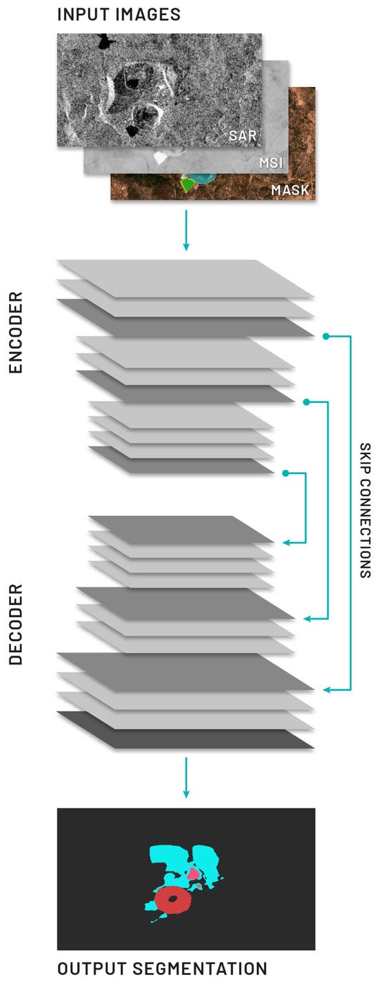
Figure 4.
An illustration of encoder–decoder network for semantic segmentation using multidimensional, satellite images.
Supervised image segmentation using deep learning requires a substantial amount of labeled data. To address this, we partitioned the set of labels into three non-overlapping subsets mentioned in Section 2.2, thereby avoiding the need for more complex multi-label segmentation. We also developed a general model capable of detecting areas covered by any label, i.e., total transformed area. Table 2 presents the number of datasets created, with Models 1, 2, and 3 consisting of detailed labels, and Model 4 comprising a single general label. We begin by selecting the optimal band configuration for each model using semantic segmentation metrics. Once we have determined the best configuration, we proceed to conduct tests using this configuration to select the most suitable dataset split.
Table 2.
A comparative analysis of dataset size using splits based on the type of extracted raw material, including coal and lignite (CL), metallic ores (MO), and rock raw materials (RR), as well as splits based on surface mine types, such as opencast (OC), open-pit (OP), and mountain-top (MT).
Each location in the dataset was labeled with a time series consisting of around five examples. To ensure the integrity of our results and prevent data leakage, we divided the training, validation, and test datasets based on mine location using a 70:15:15 ratio. During the data splitting process, all examples of the time series for each mine location were included in the training dataset. This decision was made to provide our machine learning models with a comprehensive understanding of the temporal patterns and dynamics associated with each mine location. However, in order to evaluate the performance of our models objectively, we included only one image from the time series for each mine location in the validation and test datasets.
2.4. Experiments
All models were trained using the transfer learning method, a widely used approach in deep learning. Specifically, we used the well-known ++ [18] architecture with [19] backbone. During training, we set the batch size to 4, the learning rate to , and the image size to pixels. Each model was trained for 150 epochs to ensure convergence and optimal performance. We employed various data augmentation techniques during training to improve the model’s ability to generalize to new data. Specifically, all images were normalized, randomly cropped, and augmented three times using horizontal and vertical flips, as well as 90-degree rotations. During testing, images were normalized and center-cropped to maintain consistency with the training process.
2.4.1. Band Configuration
To determine the most informative spectral bands, we investigated input band configuration, comparing five different configurations:
- RGB: Three-dimensional input, corresponds to red, green, and blue channels.
- R + N: Four-dimensional input, corresponds to RGB and near-infrared channels.
- M: Twelve-dimensional input, corresponds to all Sentinel-2 multispectral channels.
- M + S: Fifteen-dimensional input, corresponds to all Sentinel-2 multispectral bands and 3 Sentinel-1 radar channels.
- R + N + S: Seven-dimensional input, corresponds to RGB, near-infrared, and Sentinel-1 radar channels.
2.4.2. Dataset Split
Next, after selecting the optimal band configuration for each model, we conducted a comparison between two distinct data splits based on the type of extracted material: rock raw materials (RR), metal ores (MO), coal/lignite (CL), and surface mine type: open-pit (OP), opencast (OC), and mountain-top (MT). We accordingly split the dataset, trained new models, and tested on a shrunken test set. To compare general models with corresponding splits, we created two models (GM, GS) as a merge of relevant sets into one e.g., for surface mine type, we merged MT, OC, and OP datasets. Consequently, the models were trained on the entire set but exclusively tested on specific test subsets.
2.4.3. Hyperparameter Tuning
Finally, for better architecture parameter estimation, we used hyperparameter tuning. We estimated various parameter values:
- Learning rate (lr): , , .
- Batch size (bs): 4, 8, 16.
- Epochs (epc): 100, 150, 200.
- Input image size (is): 128, 256, 512.
- Optimizer (opt): sgd described in [20], adam described in [21], adamw described in [22].
- Backbone (enc): resnet50, which is a 50-layer convolutional neural network (48 convolutional layers, one MaxPool layer, and one average pool layer), vgg16 described in [23], efficientnet described in [24].
- Architectures (arc): linknet described in [25], Unet++ described in [18], deeplabv3plus described in [26], fpn described in [27], unet described in [28].
- Loss: jaccard, known as Jaccard Index, tversky described in [29], focal described in [30], crossentropy described in [31].
3. Results
We conducted a comparative analysis of four distinct performance evaluation metrics. Specifically, Intersection over Union (IoU) was employed as a measure of the accuracy of object detection on a given dataset. This metric is calculated by taking the ratio of the area of overlap between the predicted mask and the ground truth mask, and the area of their union. In addition, we considered the commonly used binary classification metrics of accuracy, recall, and precision. To account for class-specific variations in metric values, we calculated the mean values of each metric across all classes.
3.1. Band Configuration
The results of our evaluation metrics for varying input band configurations are presented in Table 3. We observed significant variability in metric values across different band configurations. Initially, we hypothesized that the R + N configuration would perform best due to its higher resolution. However, our results revealed that this configuration only outperformed the others in the binary segmentation models (2 and 4), with the addition of the near-infrared channel to the standard RGB minimally impacting the results. Differences in the metric values were generally observed only in the third decimal place.
Table 3.
A comparative analysis of selected metrics’ values for each model, trained and tested using different band configurations, including RGB (red, green, and blue channels), R+N (red, green, blue, and near-infrared channels), R + N + S (red, green, blue, near-infrared, and Sentinel-1 radar channels), M (all twelve Sentinel-2 multispectral channels), and M + S (all twelve Sentinel-2 multispectral and Sentinel-1 radar channels).
In Models 1 and 3, the inclusion of additional channels was necessary to accommodate the higher number of classes being predicted. Model 1, which predicts three classes, yielded the best results for IoU values with all multispectral band configurations. Differences in other metrics, such as accuracy, were either minor or non-existent.
In contrast, for Model 3, which predicts the highest number of classes (eight), we observed that utilizing the maximum number of channels available led to superior performance. This effect was observed across nearly all metrics, except accuracy, where differences were negligible.
3.2. Dataset Splits
Table 4 presents our metric results for varying data splits. In nearly all cases, we observed that the general models outperformed the targeted ones across all the metrics. To obtain a better understanding of the partitioning requirement, we compared with , and with . The average values represent the consequences of employing three models as an alternative to a singular model. In all instances, it was observed that utilizing a singular model was superior.
Table 4.
A comparative analysis of selected metric values for each model trained and tested on splits based on the type of extracted raw material, including coal and lignite (CL), metallic ores (MO), and rock raw materials (RR), as well as splits based on surface mine types, such as opencast (OC), open-pit (OP), and mountain-top (MT). Additionally, the table shows the results for general models, trained on the combined data from splits based on the type of extracted raw material (CL+MO+RR), and tested on rock raw materials (GRR), coal and lignite (GCL), metallic ores (GMO), as well as splits based on surface mine types (OC+OP+MT), and tested on opencast (GOC), open-pit (GOP), and mountain-top (GMT).
However, two exceptions were noted: RR and OP. In these instances, the results were either comparable or superior to those of the general models. We speculate that these splits may have been more effective for optimizing network parameters due to their larger sample sizes (Table 2). For Model 1, both smaller models yielded better results, while for Models 2 and 3, the most significant differences were observed in the recall metrics. Model 4 displayed negligible differences across all the metrics, leading us to conclude that increased data volume leads to improved model performance. We speculate that, with even more extensive data volumes, smaller models may outperform the general model.
3.3. Hyperparameter Tuning
After analyzing the optimal band configuration and recognizing the positive correlation between increased data volume and improved model performance, we proceeded to fine-tune our models through a rigorous process of 200 trials across all the datasets. The resulting hyperparameter values, optimized for maximum Intersection over Union (IoU) metric values on the test set, are presented in Table 5.
Table 5.
The optimal hyperparameters, including learning rate (lr), batch size (bs), number of epochs (epc), input image size (is), optimizer (opt), backbone (bcb), architecture (arc), and loss for comparing models with the optimal band configuration using Intersection over Union values.
Our experiments revealed that increasing the number of epochs and decreasing the learning rate consistently led to superior outcomes. However, we observed significant variances in model performance based on the specific network architecture employed. Hence, fine-tuning the hyperparameter is a critical step in achieving optimal model performance, with the complexity of the model determining the appropriate values required to maximize metric values.
4. Qualitative Analysis of the Results
In our study, we assessed machine learning model predictions for different locations using test datasets and compared them to ground truth segmentation masks.
We individually examined each label category, analyzing metric values. Below, we share notable examples that encourage discussions and conclusions, focusing extensively on key classes like excavation and dumping ground i.e., excavation and dumping ground.
4.1. Model 1 Assessment: Excavation and Preparatory Works Area
Table 6 presents metrics for Model 1, which was designed to predict excavation and preparatory work area. We analyzed these across five chosen areas for insights into factors influencing the metrics. Model 1 used the full dataset, without splitting, utilizing all MSI bands.
Table 6.
The selected metric values for chosen classes in Model 1, trained on the entire dataset, evaluated on 5 specific locations from the test set.
The initial predictions for the excavation class in the Cordero Rojo Mine and Agarak Mine locations (Figure 5 and Figure 6) seemed accurate, despite relatively low metrics due to notable false positives. These metrics, however, remained relatively high compared to other locations. False positives stem from ground truth mask disparities, possibly due to flexible boundaries from object heterogeneity. Data labeling relied on human-visible imagery, with minimal use of external tools like Google Earth’s high-resolution Digital Elevation Models (DEMs) [32]. Contrastingly, the MSI-trained model used a broader band range. The training dataset covered both clearly distinguishable and challenging excavations. Interestingly, the model’s predictions sometimes outperformed manual labeling, yielding lower metrics. Notably, the excavation category exhibited false positives mainly in other transformed areas like dumping grounds. These areas share features like land transformation, topographical variations, and vegetation absence. Furthermore, dumping grounds often coexist with excavations (internal dumps). This caused false positives when labeling excavations that contained dumping ground attributes, causing predictions on other dumping grounds (external dumps).
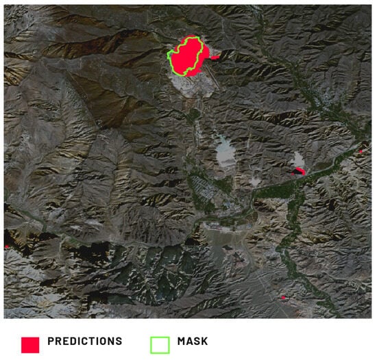
Figure 5.
Comparison of Model 1’s prediction of the excavation in the Agarak Mine, Karchevan, Armenia, against the provided ground truth mask.
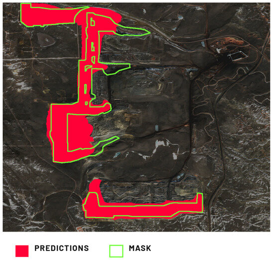
Figure 6.
Comparison of Model 1’s prediction of the excavation in the Cordero Rojo Mine, Wyoming, USA, against the provided ground truth mask.
Model 1, aside from the excavation class, was trained to predict the distinct preparatory work area class. We revealed notable false negatives in these predictions. These false negatives corresponded to simultaneous false positives in distinct excavation classes, as seen in the Cordero Rojo Mine (Figure 6 and Figure 7). Several factors could contribute to this pattern. Preparatory work areas are generally smaller than excavations, covering a thin forefront strip. Given the 10 m resolution for ground truth labeling and model training, delineation inaccuracies for excavations could span from tens to a few tens of meters, including inaccurately delineated adjacent thin preparatory work areas. Another factor could be the significant heterogeneity of the marked preparatory work areas, due to made assumptions and necessary class balance impacting prediction accuracy. Predictions often contained false positives due to earthworks or ongoing deforestation unrelated to mining, which had not been labeled as ground truth in training data.
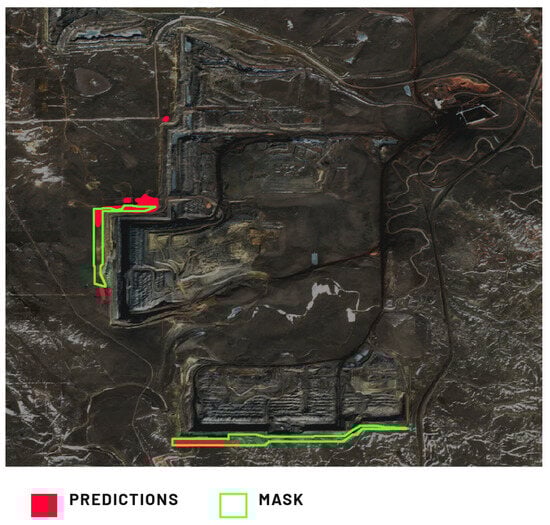
Figure 7.
Comparison of Model 1’s prediction of the preparatory work area in the Cordero Rojo Mine, Wyoming, USA, against the provided ground truth mask.
The Tunstead Quarry (Figure 8) provides a compelling case for analysis, representing a multi-pit mining site. The model accurately predicts the easternmost excavation, demonstrating alignment with the ground truth mask. Initial observations indicate accurate predictions for the other two excavations. Notably, the model correctly avoids predicting the reclaimed, water-flooded portions, in line with our assumptions. However, this area contains significant false negatives. These can be attributed in part to experts occasionally relying on external sources like Google Earth’s DEMs for annotation. Such data allowed for the identification of excavation boundaries, encompassing historic excavations with various features not prevalent in the training dataset. These features include small internal dumping grounds, resource stockpiles, and substantial infrastructure associated with mineral processing, which dominate the excavation interior. The model’s inaccurate predictions compared to the expert annotations reduced the model metrics. In this instance, human expertise, supplemented by external data, more precisely delineated excavations than the MSI-trained model. Notably, if we hypothetically replaced the excavation label with an active mining area label, predictions for this location would be nearly flawless.
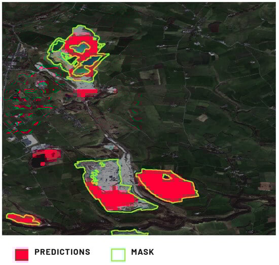
Figure 8.
Comparison of Model 1’s prediction of the excavation in the Tunstead Quarry, Buxton, UK, against the provided ground truth mask.
While assessing the results, we seldom found highly inaccurate or absent predictions, yielding IoU values close to 0 (3 out of 38 areas of the test dataset). Particularly, when analyzing the Cerovo Mine location, such cases were linked to snow presence in images. Notably, our training dataset lacked images with snow or cloud cover. Nonetheless, the recall metric remained high for this location, as the actual excavation was accurately inferred.
Our goal was to encompass a wide array of object diversity, notably, excavations, spanning large coal or metallic ore pits to smaller sandpits and distinctive bauxite excavations. Each type was deliberately included in our dataset. The model effectively inferred bauxite excavations in the Noranda Mine (Figure 9), yielding a notable recall metric. However, including these varied excavation types in the training dataset likely led to false positives in other test locations, consequently affecting the metric values.
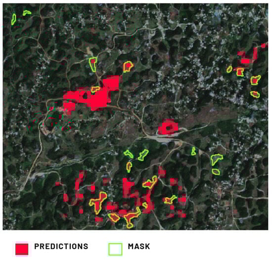
Figure 9.
Comparison of Model 1’s prediction of the excavation in the Noranda Mine, Jamaica, against the provided ground truth mask.
4.2. Model 2 Assessment: Dumping Ground
Table 7 presents metrics for Model 2, which was designed to predict dumping grounds. We analyzed these across four chosen areas for insights into factors influencing metrics. Model 2 used the full dataset, without splitting, utilizing bands.
Table 7.
The selected metric values for chosen classes in Model 2, trained on the entire dataset, evaluated on 5 specific locations from the test set.
The Rudnichny Mine (Figure 10) exhibited the most favorable metric values. Notably, it accurately captured boundaries between dumping grounds and reclaimed/untransformed areas, mostly covered by trees in this location. This precision is evident in the external dump towards the east, where forested portions coexist. While the predictions are accurate, our visual assessment identified a notable false positive within the inner dumping ground. However, this is not a model prediction error but stems from an internal dumping ground omission during dataset creation. Similar to Model 1’s approach to excavations, Model 2’s training dataset encompassed distinguishable dumping grounds and challenging cases. Consequently, we observe that predictions sometimes better align with reality than manually labeled ground truth, albeit leading to decreased model metrics for such cases.
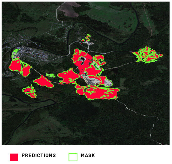
Figure 10.
Comparison of Model 2’s prediction of the dumping ground in the Rudnichny Mine, Kemerovo Oblast, Russia, against the provided ground truth mask.
The Novotroitsk Quarries (Figure 11) location displays relatively low metrics, attributed to expert labeling that classified reclaimed sections of dumps as dumping ground. Conversely, the model identified revegetated dumping grounds missed by experts and did not mark them. Our assumptions focused on not-yet vegetated dump sections, aiming to avoid potential problems of predicting undisturbed forested areas as dumps at a later stage. Also, in this case, additional false positives emerged, such as incorrect predictions of dumping grounds within excavations, likely due to shared features between dumps and excavations, as discussed in Section 4.1.
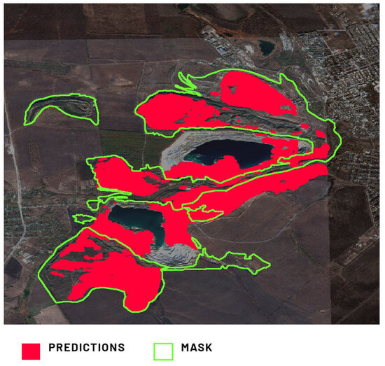
Figure 11.
Comparison of Model 2’s prediction of the dumping ground in the Novotroitsk Quarries, Donetsk Oblast, Ukraine, against the provided ground truth mask.
The Kostolac Mine location (Figure 12) presents notably low metrics. Two main observations arise. Firstly, a high-precision metric indicates most of the predictions within ground truth masks. Nonetheless, a significant false positive occurs in the excavation area due to shared features between dumping grounds and the excavation in this location. This is especially relevant in overburden removal regions where the extracted material goes directly to the dump. Secondly, numerous false negatives pertain to old TSFs, labeled by experts as dumping grounds. The scarcity of such instances in the training dataset explains the lack of prediction in these kinds of areas.
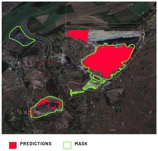
Figure 12.
Comparison of Model 2’s prediction of the dumping ground in the Kostolac Mine, Braničevo, Serbia, against the provided ground truth mask.
Model 2’s inference on non-solid wastes presents challenges due to the interplay between TSFs and dumping grounds. Experts labeled satellite images as dumping grounds, often encompassing TSFs with embankments, as both are waste and can involve overburden material from excavations. Despite varying forms, this relationship significantly impacted the metrics, exemplified by the Kovdor Mine location (Figure 13). Model 2 performed well for classic solid waste material dumps. However, a substantial false positive area emerged, possibly attributable to expert labeling subjectivity. This is compounded by the potential overlap with TSF and dam labels in Model 3’s training dataset.
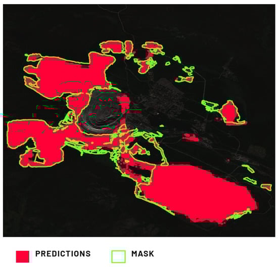
Figure 13.
Comparison of Model 2’s prediction of the dumping ground in the location of the Kovdor Mine, Murmansk Oblast, Russia, against the provided ground truth mask.
4.3. Model 3 Assessment: Other Components of Mining Areas
Table 8 presents metrics for Model 3, which was designed to predict tailing storage facility (TSF), settling pond, infrastructure (Infra), dam, stockpile exploitation slope, and transportation slope. We analyzed these across three chosen areas for insights into factors influencing the metrics. Model 3 used the full dataset, without splitting, utilizing bands.
Table 8.
The selected metric values for chosen classes in Model 3, trained on the entire dataset, evaluated on 3 specific locations from the test set.
Model 3 was devised for predicting mining area components, less prevalent than excavations and dumping grounds. Importantly, not all Model 3 classes correspond to each mining area. The Buenavista Mine (Figure 14) location illustrates this, with experts labeling components such as TSF, infrastructure, settling pond, and dam, mirrored in Model 3’s predictions. The absence of other designated land cover classes is a notable observation. In our training dataset, some Model 3-specific classes, like exploitation slope and transportation slope, occurred infrequently, mainly relevant for certain types of surface mines like opencast coal mines.
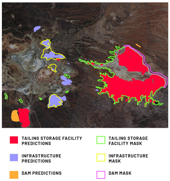
Figure 14.
Comparison of Model 3’s prediction of infrastructure, TSF, and dam in the location of the Buenavista Mine, Cananea, Mexico, against the provided ground truth mask.
At the Buenavista Mine location (Figure 14), numerous false negatives occurred for the TSF class. This could be due to waste material’s diverse composition and aggregation states, encompassing liquid and sludge phases. Additionally, a substantial false positive emerged in the southern region, where a PV panel-equipped dumping ground was misclassified as a TSF. The infrastructure class exhibited excellent precision, marred only by a minor false positive, attributed to non-mining-related infrastructure that had not been marked by experts. For the entire test set, this type of false positive was the primary reason for decreased metrics for the infrastructure label and the overall model. At Buenavista Mine, false negatives were predominantly due to experts labeling diverse objects as infrastructure, while the model’s predictions targeted evident infrastructure elements recurring in the training dataset. Similarly, the settling pond class yielded numerous false negatives, as these small objects often went unrecognized by the model. Problematically, the dam class exhibited a large false positive in untransformed areas. This could stem from many dams in the training dataset being earth dams, sharing features with completely untransformed regions.
The Globe–Miami Mining District (Figure 15) shows false positives of the TSF class. The model’s prediction also includes a dam on the tailings. We find the reasons for this model inference lies in the difficulties of experts in correctly determining the boundary between the real water table of a TSF and its dam on 10 × 10 m resolution images.
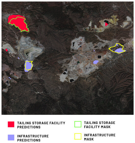
Figure 15.
Comparison of Model 3’s prediction of the infrastructure and TSF in the Globe–Miami Mining District, Arizona, USA, against the provided ground truth mask.
We observed similar prediction results in the Bor Mine (Figure 16) location, where for the infrastructure and TSF classes, the causes of both false positives and false negatives are similar to previous examples. At this location, however, the prediction for the dam class seems to be very good, with a precision metric close to 1. This is the type of earth dam that appeared most often in the training set, which resulted in better metrics.
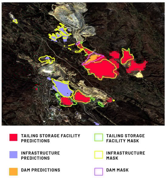
Figure 16.
Comparison of Model 3’s prediction of the infrastructure, TSF, and dam in the Bor Mine, Bor, Serbia, against the provided ground truth mask.
4.4. Visual Check of the Results
As we expect our models to be useful for several use cases (land use monitoring, detection of illegal mining, and mining plans verification). We carefully analyzed some prediction examples in terms of their factual correctness. In most cases, the predictions are not perfect but remain promising. In Figure 17 and Figure 18 we present a comparison of predictions for the chosen area, on satellite images separated by a two-year interval.
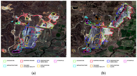
Figure 17.
Example predictions of mining area components within the Bengala Coal Mine (Australia) of Model 1, Model 2, and Model 3 for 2019 (a) and 2021 (b).
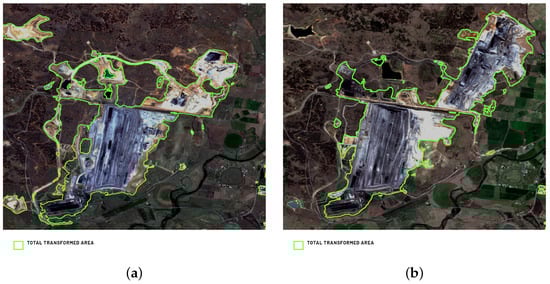
Figure 18.
Example predictions of the total transformed area within the Bengala Coal Mine (Australia) of Model 4 for 2019 (a) and 2021 (b).
Although not ideal, the obtained results are often sufficient for their general interpretation in terms of the verification of long-term mining plans. The presented predictions describe the mining area of the Bengala Coal Mine in Australia. In 2021, we see a significant increase in the area of the excavation and dumping ground in the northeastern direction, compared to 2019. This is the result of the creation of a new excavation and the progress of mining works. There is also a significant increase in the area of dumps as a result of both external and internal dumping.
A visual inspection confirms the good metrics for Model 4 in almost all the cases, correctly predicting the total transformed area. This confirms the possibility of using the results for mining land use monitoring as well as for illegal mining detection.
5. Discussion
Based on the metric values obtained throughout the entire research and later qualitative analysis of the results, we find several topics worth discussing before stating our final conclusions.
5.1. The Approach to Label Selection and Definition
Each mining area is unique, making it challenging to create universal models for predicting such diverse objects. The obtained models’ metrics were influenced by the heterogeneity of the objects. In some cases, there were other defined classes present within the excavations or dumping grounds, such as internal dumping grounds, stockpiles, and infrastructure. Consequently, the models considered the characteristic features of these internal components, sometimes leading to false positives when these components were outside the excavation in the test dataset. One potential solution is to optimize the selection and definition of mining land cover classes, such as using labels like active exploitation area and active dumping area instead of excavation and dumping ground, respectively. This approach would prevent objects from exhibiting features related to multiple classes simultaneously. Alternatively, a less comprehensive approach could be considered, allowing for more specific labels by not aiming to mark every smallest fragment of the transformed area, particularly in Models 1 and 2.
5.2. Universal vs. Split Datasets
Developing universal models for all surface mines and related facilities is debatable. Our research neither confirms nor excludes this possibility. Balancing models’ accuracy and universality is crucial. Clearly defining available resources during research is essential. In our study, assumptions and compromises influenced the obtained models’ metrics. One assumption was capturing the entire mining-transformed area during satellite image labeling to assess the total mining land use. As one of the compromises, we can point to the approach to TSF labeling, where TSF itself treated the water/sludge surface of the tailings, while the entire facility was still treated as a dumping ground. In some specific cases (when the tailings were dammed only on one side), the dam class was used. To reduce heterogeneity, we split the training data by raw material type and surface mine type. Although the new models did not significantly improve prediction quality, the validity of dataset splitting cannot be disregarded.
5.3. Heterogenity of Mining Areas vs. Randomness of Test Dataset Locations
The random selection of mining areas for the test dataset significantly influenced the metrics due to class diversity. Our research heavily relies on metric values, which could vary significantly with a different test dataset. Including typical mining areas may yield significantly higher or lower metrics. Model 3’s metrics were affected by the presence or absence of specific mining land cover classes in the locations. Classes like dam, exploitation slope, transportation slope, and stockpile were optional and applicable only to specific mining areas.
5.4. Incorporation of Satellite Data with Higher Spatial Resolution
Our qualitative analysis revealed that the spatial resolution of the images posed limitations on the experts’ ability to accurately delineate boundaries between different mining components. Problematic areas included the borders between dumping grounds and untransformed/reclaimed areas, excavations, and preparatory work areas, and TSFs and dams. The utilization of improved spatial resolution data in similar studies would significantly reduce subjectivity among experts and provide more precise markings. Additionally, we observed that the models faced challenges (lower metrics confirmed by visual analysis) in capturing objects with very small surface areas, such as rock quarries, which have smaller transformed areas compared to metallic ore or coal mines. Conducting similar studies using satellite data of a higher spatial resolution could potentially enhance the object recognition accuracy. This proposition, however, necessitates further investigation.
5.5. Application of Additional Conditions
We see several possibilities to improve the operation and practical application of the developed models. One option is to set specific conditions for model predictions, such as limiting the area prediction to the preparatory works adjacent to the excavation or considering a dam as a polygon adjacent to the TSF. Integrating our models with conventional land use and land cover (LULC) models is another idea that can help reduce false positives outside transformed areas. These strategies hold promise for improving the overall performance and applicability of our models.
5.6. Limitations of the Presented Study
The research and testing of machine learning models for the segmentation of mining facilities focused exclusively on images depicting large mines and their adjacent areas. There was no evaluation of these models on images featuring earthworks unrelated to mining, such as archaeological sites, construction sites, etc. Consequently, the assessments and conclusions drawn do not extend to the models’ effectiveness in non-mining contexts.
6. Conclusions
In the task of mining area segmentation using machine learning techniques, for our assumptions, data, and techniques, we explored various approaches and arrived at the following conclusions.
Different machine learning models were employed to identify individual components of mining areas, RGB achieving the best metrics with specific band combinations. For the binary models (Models 2 and 4), the RGB + NIR band combination yielded the best results, whereas, for the multiclass models, the composition of all the multispectral bands (Model 1) or the composition of the multispectral and radar bands (Model 3) proved more effective. However, none of the tested combinations demonstrated a clear advantage over the others, with the differences often being marginal. This could imply that as the number of labels in the dataset increases, there is a corresponding need for a greater number of bands. Nevertheless, in this context, data fusion did not significantly enhance the segmentation process. Given that some of the defined classes in the Model 3 are associated with water (TSF, settling pond), the advantage of the model using radar data seems to be justified.
The dataset splits based on extracted raw material type and surface mine type did not substantially improve the models’ performance metrics. In contrast to the models designed for particular mine types and extracted raw material types, the general model exhibited better performance. However, Model 1, dedicated to rock row material type (RR) and opencast type (OC) mining, demonstrated a significant improvement over the general model, which may be attributed to the availability of a larger sample size. It is important to mention that despite the variations in mining areas, models trained exclusively for specific mine types did not outperform the general model. However, we cannot deny or confirm the pertinence of splitting datasets in this way and we recommend repeating similar studies on a larger sample of training data.
Model 4, which we created to predict an entire transformed area, performs effectively, as demonstrated by the metrics. This indicates that the combination of satellite imagery and machine learning models offers a viable approach to developing a robust tool for monitoring land transformations caused by mining operations. Our findings suggest that the current iteration of the model can detect illegal mining activities and facilitate the comprehensive monitoring of land use. The authors in [9,10] utilized a model with an accuracy of 88.4% to construct the global dataset of mining areas. In contrast, our best model achieved a significantly higher accuracy of 96%.
Although separating the individual components of a mining area remains a challenge, the existing models dedicated to this task are not yet suitable for operational activities. Nevertheless, it is essential to acknowledge the potential of existing models and the possibility of improving their performance by expanding and diversifying the dataset. Consistent efforts toward expanding the self-prepared dataset can increase the training set, thereby resulting in positive outcomes for the models. Also, conducting a similar study on higher-spatial-resolution satellite data may significantly improve the results.
The need for effective land use monitoring in mining areas is emphasized due to increased raw material demand and growing environmental awareness. Understanding land transformation in mining leads to sustainable resource management and operational optimization. This study contributes to the area of space-borne data analysis using machine learning methods and has shown that utilizing RGB channels in satellite images is sufficient for the precise identification and monitoring of mining areas. Our findings suggest that the incorporation of all multispectral bands or division of the dataset based on surface mine type or extracted materials is not necessary, and a generalized model can achieve optimal accuracy and efficiency. Moreover, our research highlights the potential of employing machine learning models and satellite data in monitoring mining areas. These powerful tools can provide invaluable insights into mining operations and their impact on the environment. The implications of our findings are significant for both the mining industry and professionals in remote sensing and machine learning research.
Author Contributions
Conceptualization, K.J., M.M., D.T., W.K., M.Z. and M.W.; methodology, K.J., M.M., D.T. and M.Z.; software, K.J.; validation, M.M., D.T. and W.K.; formal analysis, D.T., W.K., M.Z. and M.W.; investigation, K.J., M.M., D.T., W.K. and M.Z.; resources, M.W.; data curation, K.J., M.M. and M.W.; writing—original draft, K.J., M.M., D.T. and W.K.; writing—review and editing, K.J., M.M., D.T., W.K. and M.Z.; visualization, K.J.; supervision, K.J. and M.W.; project administration, K.J. and M.W.; funding acquisition, M.W. All authors have read and agreed to the published version of the manuscript.
Funding
This research was funded by the National Centre for Research and Development.
Institutional Review Board Statement
Not applicable.
Informed Consent Statement
Not applicable.
Data Availability Statement
Embargo on data due to commercial restrictions.
Acknowledgments
We acknowledge Paulina Dziubek and Makary Musiałek for data annotations, Michał Wierzbiński for advising on machine learning model training, and Agnieszka Mazurkiewicz and Edyta Lewicka for creating graphics. This research was supported by the European Fund. The developed models were implemented into the TerraEye application, owned by Remote Sensing Business Solutions [33].
Conflicts of Interest
Authors Katarzyna Jabłońska, Wojciech Kaczan and Marek Wilgucki are employed by the company Remote Sensing Business Solutions. Authors Marcin Maksymowicz and Dariusz Tanajewski are employed by the company Remote Sensing Environmental Solutions. The remaining authors declare that the research was conducted in the absence of any commercial or financial relationship that could be construed as a potential conflict of interest.
References
- Delevingne, L.; Glazener, W.; Grégoir, L.; Henderson, K. Climate Risk and Decarbonization: What Every Mining CEO Needs to Know; McKinsey & Company: New York, NY, USA, 2020; Available online: https://www.mckinsey.com/capabilities/sustainability/our-insights/climate-risk-and-decarbonization-what-every-mining-ceo-needs-to-know (accessed on 10 January 2024).
- Loh, Y.W.; Mohammad, A.; Tripathi, A.; van Niekerk, E.; Yanto, Y. Advancing Metals and Mining in Southeast Asia with Digital and Analytics; McKinsey & Company: New York, NY, USA, 2023; Available online: https://www.mckinsey.com/industries/metals-and-mining/our-insights/advancing-metals-and-mining-in-southeast-asia-with-digital-and-analytics (accessed on 10 January 2024).
- Mononen, T.; Kivinen, S.; Kotilainen, J.M.; Leino, J. Social and Environmental Impacts of Mining Activities in the EU 2022. Available online: https://www.europarl.europa.eu/RegData/etudes/STUD/2022/729156/IPOL_STU(2022)729156_EN.pdf (accessed on 10 January 2024).
- Environmental Law Alliance Worldwide. Guidebook for Evaluating Mining Project EIAs; Environmental Law Alliance Worldwide: Eugene, OR, USA, 2010; Available online: https://elaw.org/resource/guidebook-evaluating-mining-project-eias (accessed on 10 January 2024).
- Nascimento, F.S.; Gastauer, M.; Souza-Filho, P.W.M.; Wilson, R.; Nascimento, J.; Santos, D.C.; Costa, M.F. Land Cover Changes in Open-Cast Mining Complexes Based on High-Resolution Remote Sensing Data. Remote Sens. 2020, 12, 611. [Google Scholar] [CrossRef]
- Asner, G.P.; Llactayo, W.; Tupayachi, R.; Luna, E.R. Elevated rates of gold mining in the Amazon revealed through high-resolution monitoring. Proc. Natl. Acad. Sci. USA 2013, 110, 18454–18459. [Google Scholar] [CrossRef] [PubMed]
- Chen, W.; Li, X.; He, H.; Wang, L. A Review of Fine-Scale Land Use and Land Cover Classification in Open-Pit Mining Areas by Remote Sensing Techniques. Remote Sens. 2018, 10, 15. [Google Scholar] [CrossRef]
- Sonter, L.J.; Barrett, D.J.; Soares-Filho, B.S.; Moran, C.J. Global demand for steel drives extensive land-use change in Brazil’s Iron Quadrangle. Glob. Environ. Chang. 2014, 26, 63–72. [Google Scholar] [CrossRef]
- Maus, V.; Giljum, S.; Gutschlhofer, J.; da Silva, D.M.; Probst, M.; Gass, S.L.B.; Luckeneder, S.; McCallum, M.L.I. A global-scale data set of mining areas. Sci. Data 2020, 7, 289. [Google Scholar] [CrossRef] [PubMed]
- Maus, V.; Giljum, S.; da Silva, D.M.; Gutschlhofer, J.; da Rosa, R.P.; Luckeneder, S.; Gass, S.L.B.; Lieber, M.; McCallum, I. An update on global mining land use. Sci. Data 2022, 9, 433. [Google Scholar] [CrossRef] [PubMed]
- Balaniuk, R.; Isupova, O.; Reece, S. Mining and Tailings Dam Detection in Satellite Imagery Using Deep Learning. Sensors 2020, 20, 6936. [Google Scholar] [CrossRef]
- Yu, X.; Zhang, K.; Zhang, Y. Land use classification of open-pit mine based on multi-scale segmentation and random forest model. PLoS ONE 2022, 17, e0263870. [Google Scholar] [CrossRef]
- Maxwell, A.E.; Warner, T.A.; Strager, M.P.; Conley, J.F.; Sharp, A.L. Assessing machine-learning algorithms and image- and lidar-derived variables for GEOBIA classification of mining and mine reclamation. Int. J. Remote Sens. 2015, 36, 954–978. [Google Scholar] [CrossRef]
- Mukherjee, J.; Mukherjee, J.; Chakravarty, D.; Aikat, S. A Novel Index to Detect Opencast Coal Mine Areas From Landsat 8 OLI/TIRS. IEEE J. Sel. Top. Appl. Earth Obs. Remote Sens. 2019, 12, 891–897. [Google Scholar] [CrossRef]
- Karan, S.K.; Samadder, S.R.; Maiti, S.K. Assessment of the capability of remote sensing and GIS techniques for monitoring reclamation success in coal mine degraded lands. J. Environ. Manag. 2016, 182, 272–283. [Google Scholar] [CrossRef]
- Demirel, N.; Düzgün, Ş.; Emil, M.K. Landuse change detection in a surface coal mine area using multi-temporal high-resolution satellite images. Int. J. Min. Reclam. Environ. 2011, 25, 342–349. [Google Scholar] [CrossRef]
- Maxwell, A.E.; Warner, T.A. Differentiating mine-reclaimed grasslands from spectrally similar land cover using terrain variables and object-based machine learning classification. Int. J. Remote Sens. 2015, 36, 4384–4410. [Google Scholar] [CrossRef]
- Zhou, Z.; Siddiquee, M.M.R.; Tajbakhsh, N.; Liang, J. UNet++: A Nested U-Net Architecture for Medical Image Segmentation. In Deep Learning in Medical Image Analysis and Multimodal Learning for Clinical Decision Support; Springer: Cham, Switzerland, 2018. Available online: http://xxx.lanl.gov/abs/1807.10165 (accessed on 10 January 2024).
- He, K.; Zhang, X.; Ren, S.; Sun, J. Deep Residual Learning for Image Recognition. In Proceedings of the IEEE Conference on Computer Vision and Pattern Recognition (CVPR), Las Vegas, NV, USA, 26 June–1 July 2016. [Google Scholar] [CrossRef]
- Hardt, M.; Recht, B.; Singer, Y. Train faster, generalize better: Stability of stochastic gradient descent. In Proceedings of the 33rd International Conference on Machine Learning, New York, NY, USA, 20–22 June 2016; Available online: http://xxx.lanl.gov/abs/1509.01240 (accessed on 10 January 2024).
- Kingma, D.P.; Ba, J. Adam: A Method for Stochastic Optimization. arXiv 2017, arXiv:1412.6980. [Google Scholar] [CrossRef]
- Loshchilov, I.; Hutter, F. Decoupled Weight Decay Regularization. arXiv 2019, arXiv:1711.05101. [Google Scholar] [CrossRef]
- Simonyan, K.; Zisserman, A. Very Deep Convolutional Networks for Large-Scale Image Recognition. arXiv 2015, arXiv:1409.1556. [Google Scholar] [CrossRef]
- Tan, M.; Le, Q.V. EfficientNet: Rethinking Model Scaling for Convolutional Neural Networks. arXiv 2020, arXiv:1905.11946. [Google Scholar] [CrossRef]
- Chaurasia, A.; Culurciello, E. LinkNet: Exploiting encoder representations for efficient semantic segmentation. In Proceedings of the 2017 IEEE Visual Communications and Image Processing (VCIP), St. Petersburg, FL, USA, 10–13 December 2017; pp. 1–4. [Google Scholar] [CrossRef]
- Chen, L.C.; Zhu, Y.; Papandreou, G.; Schroff, F.; Adam, H. Encoder-Decoder with Atrous Separable Convolution for Semantic Image Segmentation. In Computer Vision—ECCV 2018; Springer: Cham, Switzerland, 2018. [Google Scholar] [CrossRef]
- Lin, T.Y.; Dollár, P.; Girshick, R.; He, K.; Hariharan, B.; Belongie, S. Feature Pyramid Networks for Object Detection. In Proceedings of the 2017 IEEE Conference on Computer Vision and Pattern Recognition (CVPR), Honolulu, HI, USA, 21–26 July 2017. [Google Scholar] [CrossRef]
- Ronneberger, O.; Fischer, P.; Brox, T. U-Net: Convolutional Networks for Biomedical Image Segmentation. In Medical Image Computing and Computer-Assisted Intervention—MICCAI 2015; Springer: Cham, Switzerland, 2015. [Google Scholar] [CrossRef]
- Salehi, S.S.M.; Erdogmus, D.; Gholipour, A. Tversky Loss Function for Image Segmentation Using 3D Fully Convolutional Deep Networks. In Machine Learning in Medical Imaging; Springer: Cham, Switzerland, 2017. [Google Scholar] [CrossRef]
- Lin, T.Y.; Goyal, P.; Girshick, R.; He, K.; Dollár, P. Focal Loss for Dense Object Detection. IEEE Trans. Pattern Anal. Mach. Intell. 2020, 42, 318–327. [Google Scholar] [CrossRef] [PubMed]
- Zhang, Z.; Sabuncu, M.R. Generalized Cross Entropy Loss for Training Deep Neural Networks with Noisy Labels. 2018. Available online: http://xxx.lanl.gov/abs/1805.07836 (accessed on 10 January 2024).
- Google Earth. Available online: https://www.google.com/earth/ (accessed on 10 January 2024).
- TerraEye. Available online: https://terraeye.co/ (accessed on 10 January 2024).
Disclaimer/Publisher’s Note: The statements, opinions and data contained in all publications are solely those of the individual author(s) and contributor(s) and not of MDPI and/or the editor(s). MDPI and/or the editor(s) disclaim responsibility for any injury to people or property resulting from any ideas, methods, instructions or products referred to in the content. |
© 2024 by the authors. Licensee MDPI, Basel, Switzerland. This article is an open access article distributed under the terms and conditions of the Creative Commons Attribution (CC BY) license (https://creativecommons.org/licenses/by/4.0/).