PolSAR Image Classification with Active Complex-Valued Convolutional-Wavelet Neural Network and Markov Random Fields

Abstract

PolSAR image classification has attracted extensive significant research in recent decades. Aiming at improving PolSAR classification performance with speckle noise, this paper proposes an active complex-valued convolutional-wavelet neural network by incorporating dual-tree complex wavelet transform (DT-CWT) and Markov random field (MRF). In this approach, DT-CWT is introduced into the complex-valued convolutional neural network to suppress the speckle noise of PolSAR images and maintain the structures of learned feature maps. In addition, by applying active learning (AL), we iteratively select the most informative unlabeled training samples of PolSAR datasets. Moreover, MRF is utilized to obtain spatial local correlation information, which has been proven to be effective in improving classification performance. The experimental results on three benchmark PolSAR datasets demonstrate that the proposed method can achieve a significant classification performance gain in terms of its effectiveness and robustness beyond some state-of-the-art deep learning methods.

1. Introduction

Recently, polarimetric synthetic aperture radar (PolSAR) [1,2] has been able to capture the polarimetric characteristics of ground targets in addition to their scattering echo amplitude, phase, and frequency characteristics; it is one of the most important remote sensing types and more sophisticated than the traditional SAR system. PolSAR obtains the target polarization scattering matrix by sending and receiving electromagnetic waves with different polarization modes in order to measure the ground target’s polarization scattering properties [3]. Terrain classification using PolSAR image data has became a very challenging interpretation task due to limited labeled samples, unexploited spatial information, and speckle noise. PolSAR terrain classification, which focuses on assigning a meaningful category to each pixel vector according to PolSAR image contents, has wide application prospects, such as sea monitoring, geological resource exploration, agriculture status assessment, navigation safety, topographic mapping, etc. [4,5,6,7].

In the last few decades, PolSAR classification has been carried out with a wide variety of machine learning methods when limited numbers of labeled samples are obtainable. Kong et al. [8] developed a Bayesian classification approach to terrain cover identification using polarimetric data. Tao et al. [9] incorporated spatial and feature information into the k-nearest neighbor (KNN) classifier for PolSAR classification. Lardeux et al. [10] successfully applied SVM for Multifrequency PolSAR classification. Ersahin et al. [11] proposed a spectral graph clustering technique to improve performance in the classification of PolSAR images. Bi et al. [12] employed discriminative clustering for unsupervised PolSAR image classification. Antropov et al. [13] adopted a probabilistic neural network (PNN) for land cover mapping using spaceborne PolSAR image data. Compared with the polarimetric decomposition technique, machine learning PolSAR classification can usually make classification performance more robust and accurate.

Recently, a group of deep learning methods for PolSAR classification have been discussed in the literature and are demonstrated to be powerful for acquiring deep representations and discriminative features from PolSAR data. Zhou et al. [14] used a deep convolutional neural network for supervised multilooked POLSAR classification. Liu et al. [15] suggested a Wishart deep belief network (W-DBN) for PolSAR classification by making full use of local spatial information. Jiao and Liu [16] designed a Wishart deep stacking network (W-DSN) for fast PolSAR classification. Zhang et al. [17] presented a complex-valued CNN (CV-CNN) for PolSAR classification by employing both amplitude and phase information. Bi et al. [18] proposed a graph-based semisupervised deep neural network for PolSAR image classification. However, the success of these deep learning methods for PolSAR classification depends on massive amounts of labeled samples, as we know that PolSAR-annotated data is difficult to obtain in actual cases since labeling samples is time-consuming and labor-intensive. Additionally, speckle noise can easily affect the classification performance of PolSAR image data. Therefore, we will essentially develop a robust PolSAR classification technique that overcomes limited labeled samples and speckle noise by integrating phase and spatial information.

To tackle the problem of limited labeled samples, active learning (AL) is a powerful strategy for PolSAR classification since it can choose the most valuable samples of unlabeled data for annotation. AL has been widely applied in PolSAR and hyperspectral remote sensing images. Tuia et al. [19] proposed two AL methods for the semiautomatic definition of training samples for remote sensing image classification and applied them and SVM to the classification of VHR optical imagery and hyperspectral data. Tuia et al. [20] introduced a survey of AL for solving supervised remote sensing image classification tasks. In the literature, AL approaches concentrate on establishing new training sets by iteratively enhancing classification performance through sampling. Samat et al. [21] presented an AL ELM algorithm with fast operation and strong generalization for quad-polarimetric SAR classification. Liu et al. [22] proposed an active object-based classification algorithm with random forest for PolSAR imagery to enhance classification performance. Bi et al. [23] integrated AL and a fine-tuned CNN to improve the performance of supervised PolSAR image classification. Additionally, Li et al. [24] applied AL and loopy belief propagation to exploit the spectral and the spatial information of hyperspectral image data. Cao et al. [25] adopted deep learning and AL methods in a unified framework for hyperspectral image classification. Thus, AL is an effective method to decrease the cost of obtaining large labeled training samples for PolSAR image classification using deep learning methods.

As for speckle noise, CNN-based and CV-CNN-based methods for PolSAR image classification cannot effectively balance classification efficiency and classification performance. The wavelet transform- and complex wavelet transform-constrained pooling layers in CNN and CV-CNN can remove the speckle noise and have a better performance in PolSAR image classification. Additionally, wavelet transform domain-based CNN and CV-CNN can preserve PolSAR image edges, sharpness, and some other structures, while CNN and CV-CNN with conventional pooling have not yet taken into consideration the structure of the previous layer. Consequently, a rising number of wavelet transform domain-based deep learning algorithms have been developed to address various computer vision issues, including object categorization, picture super-resolution, etc. De et al. [26] developed two wavelet-based edge feature enhancements in the input layer to enhance the classification performance of CNN. Liu et al. [27] adapted a multi-level wavelet CNN algorithm and applied it to image restoration, including single-image super-resolution, image denoising, and object classification. Sahito et al. [28] applied scale-invariant deep learning based on stationary wavelet transform to single-image super-resolution and captured more information on the images. Therefore, using wavelet transform domain-based CNN and CV-CNN for PolSAR image classification is probably an effective way to preserve PolSAR image edges and sharpness while suppressing speckle noise.

Motivated by the discussions above, in this paper, we investigate the application of an active complex-valued convolutional-wavelet neural network and Markov random fields (ACV-CWNN-MRFs) in PolSAR image classification. Firstly, we incorporate dual-tree complex wavelet transform into CV-CNN (CV-CWNN) for PolSAR image classification to decrease the level of speckle noise. The CV-CWNN can preserve texture structures details and effectively enhance the classification performance of PolSAR images. Secondly, to address the issue of limited labeled samples, we take advantage of the potential of CV-CWNN in an active learning scheme (ACV-CWNN). Finally, we refine the PolSAR classification maps of ACV-CWNN via Markov random fields (MRFs), which utilize spatial contextual information to characterize the local correlation and implement the smooth alignment of PolSAR image edges.

The primary contributions of this research to the PolSAR classification literature are threefold:

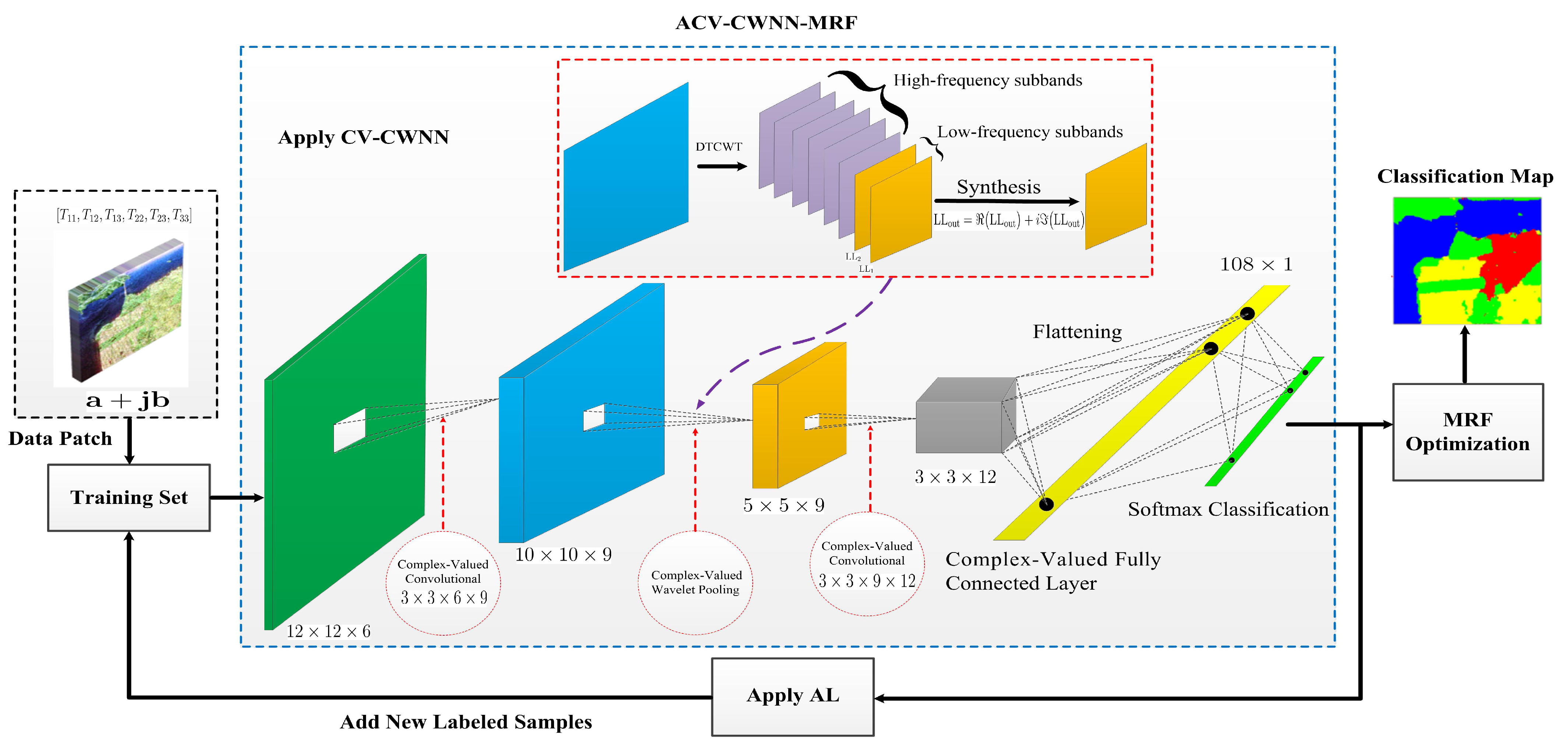
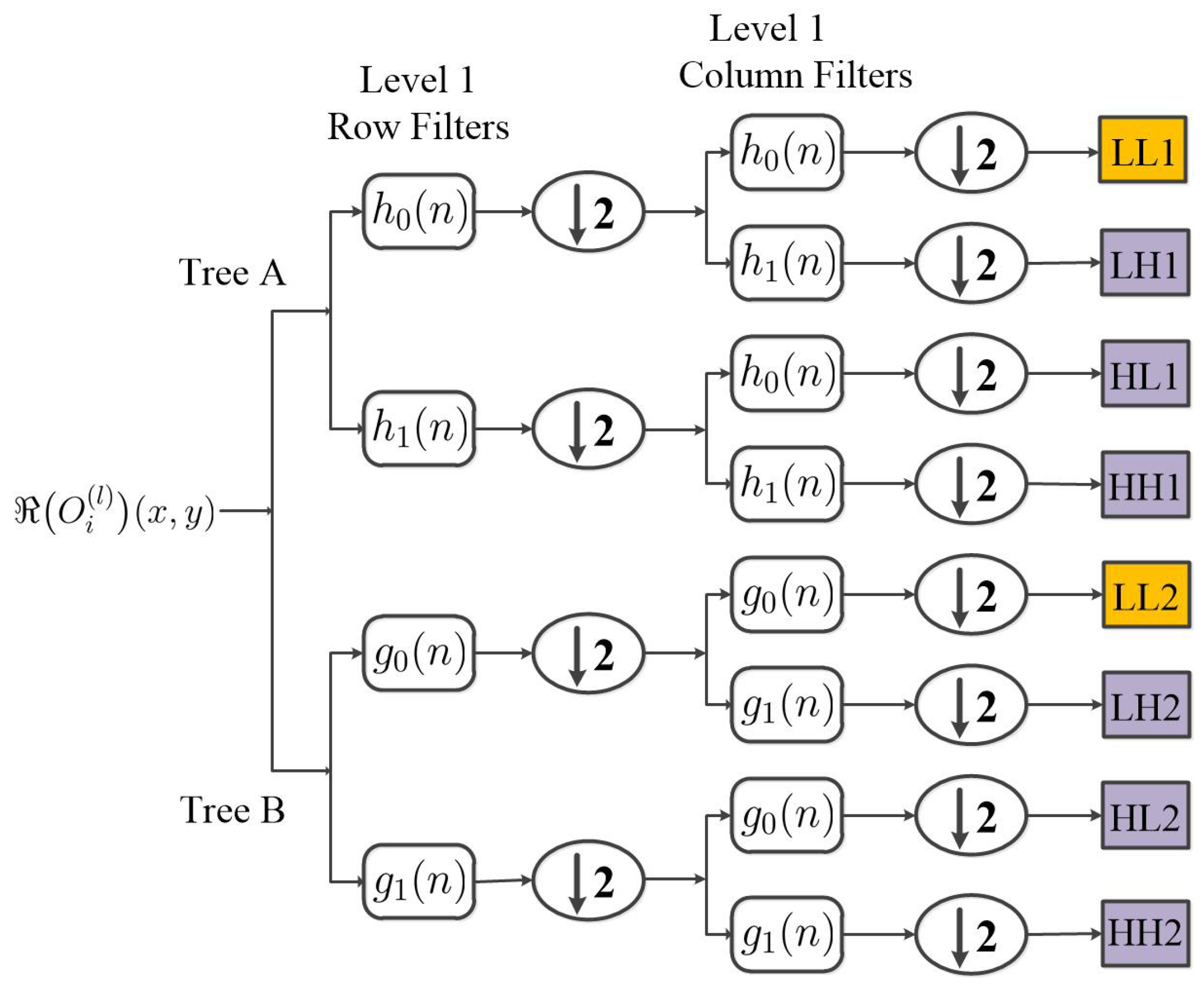
• We apply a dual-tree complex wavelet transform-constrained pooling layer to CV-CNN classification from PolSAR images to decrease the level of speckle noise and preserve some structure features (e.g., edges, sharpness) at the pooling layer.
• We integrate a combination of AL and an MRF model-based framework into CV-CWNN for the PolSAR image classification task, which not only obtains the most informative unlabeled training samples based on the output of CV-CWNN, but also achieves spatial local correlation information to improve the classification performance.
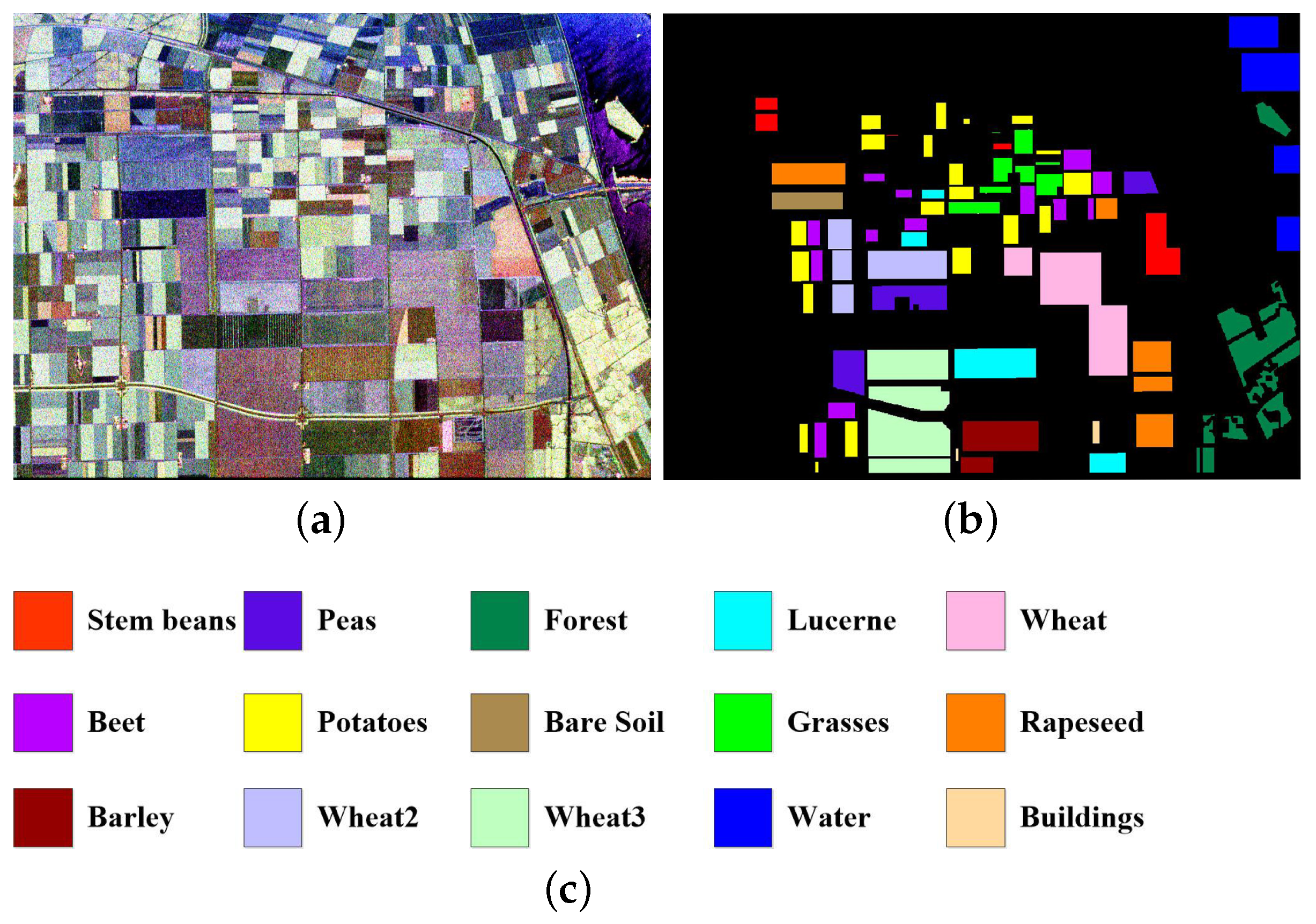
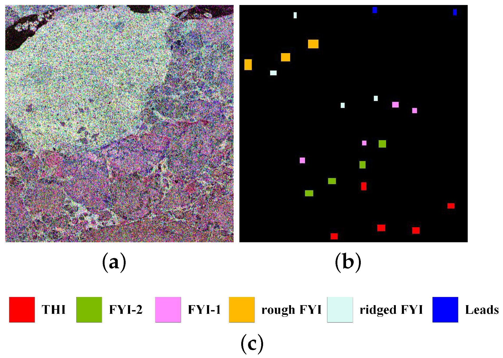
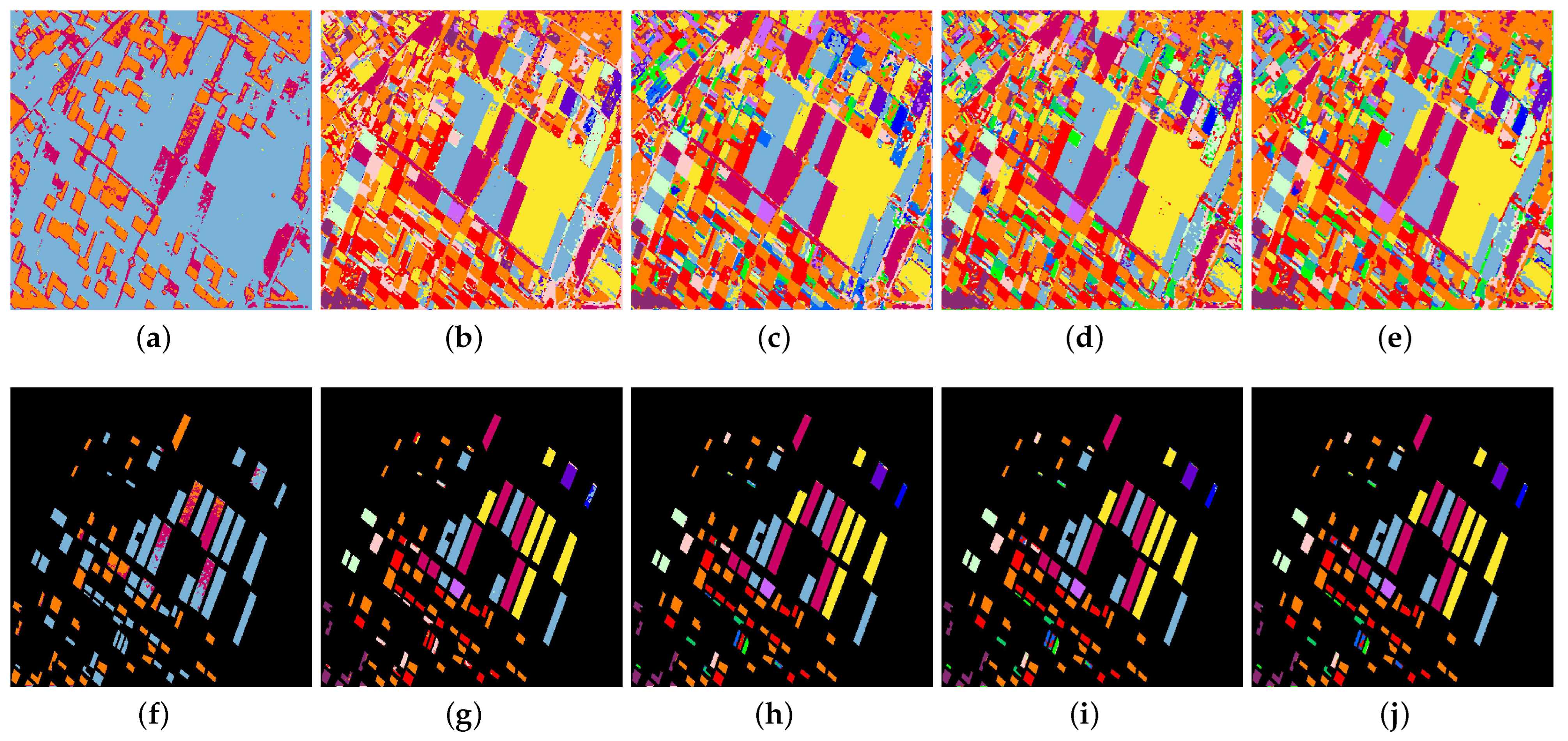
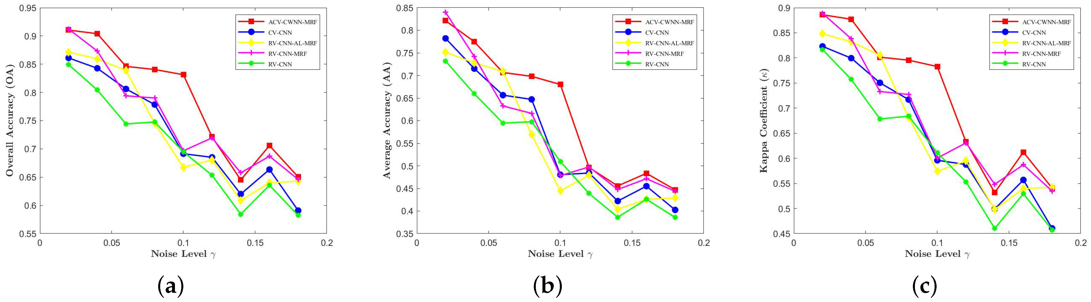
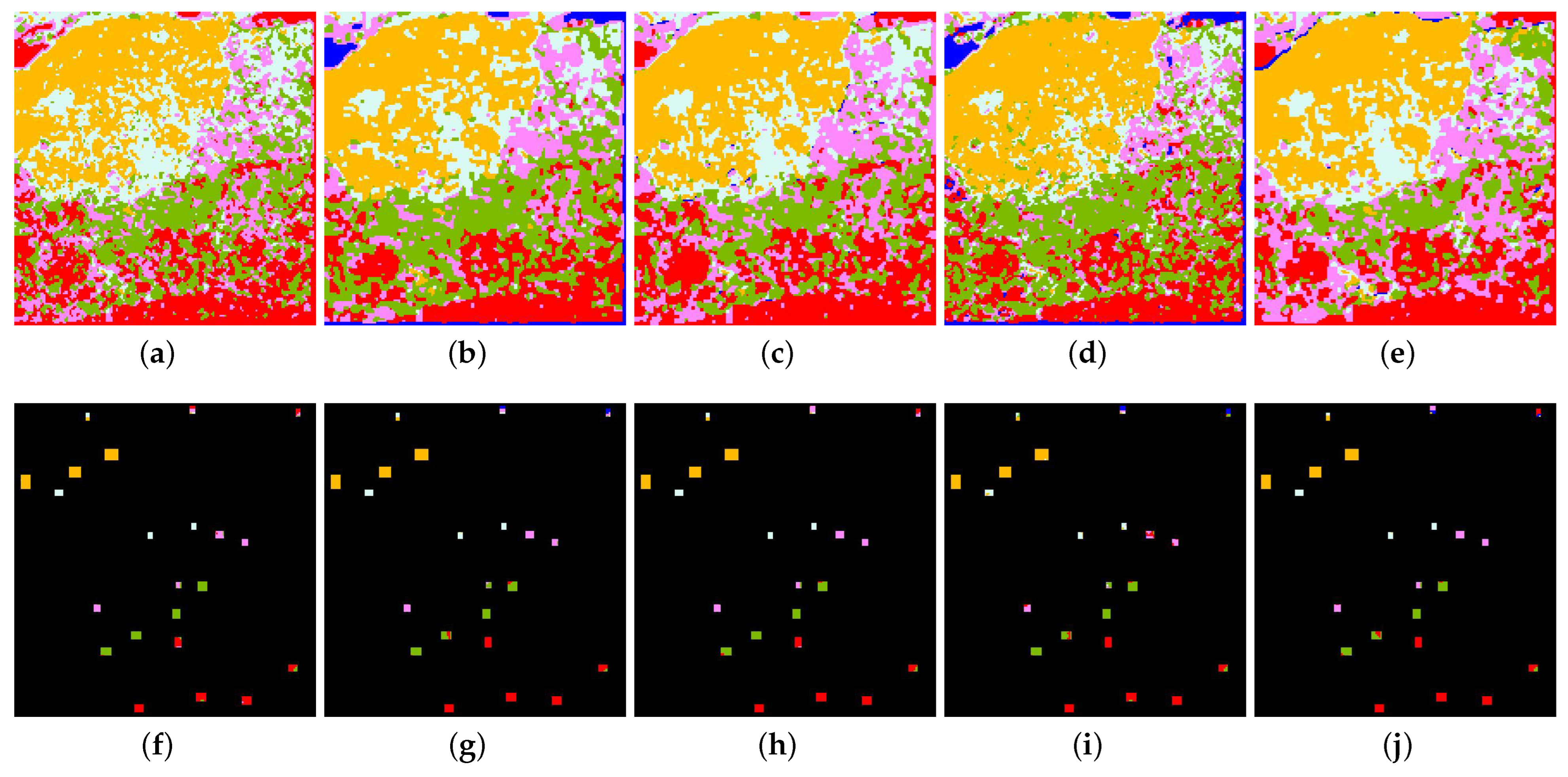
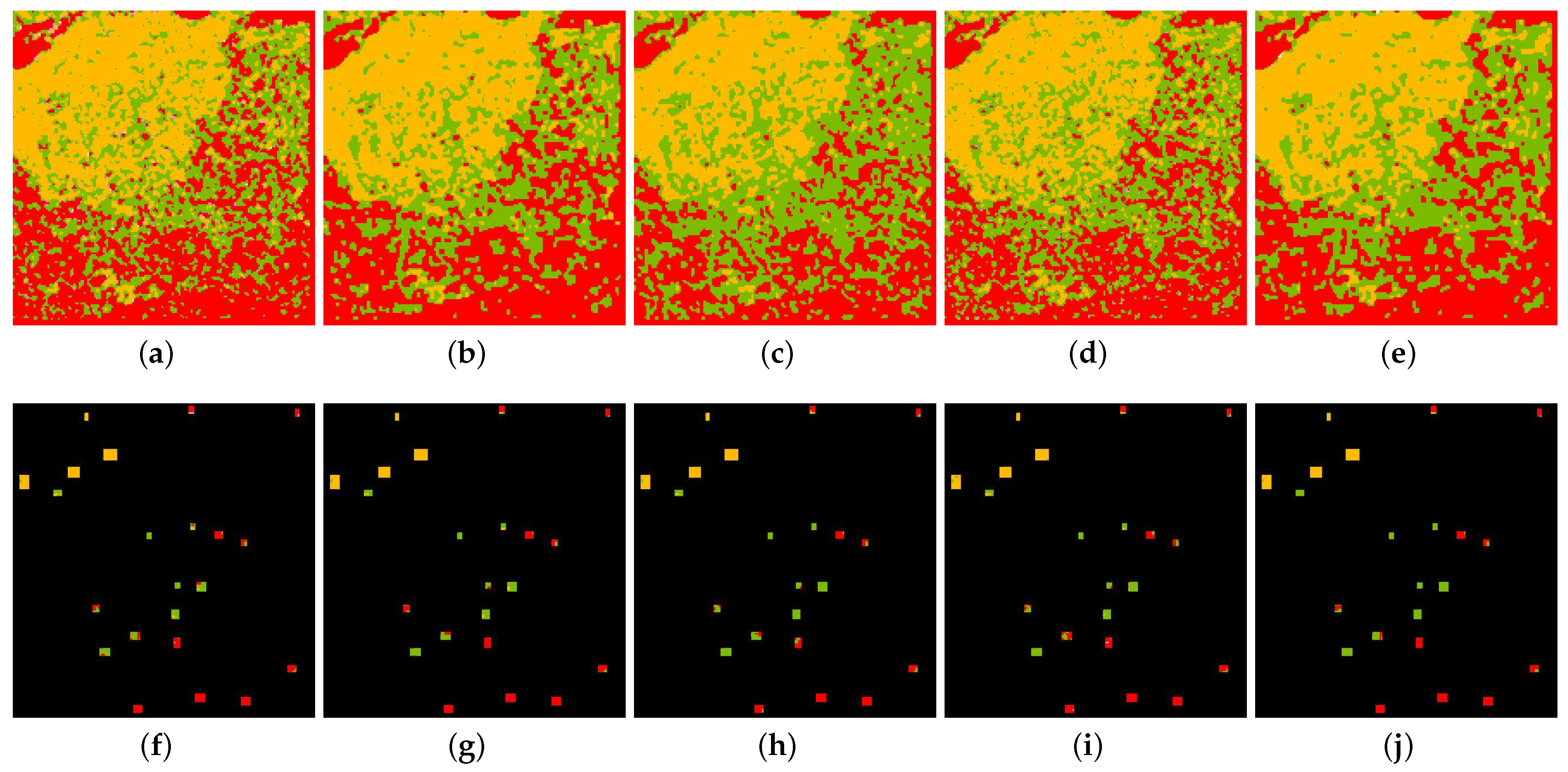
• The experimental results on several PolSAR benchmark datasets demonstrate that our proposed ACV-CWNN-MRF PolSAR classification algorithm outperforms other state-of-the-art CNN-based and CV-CNN-based PolSAR algorithms with fewer labeled samples, especially with speckle noise backgrounds.

The rest of this paper is organized as follows. In Section 2, we describe in detail the development of ACV-CWNN-MRF for PolSAR classification. In Section 3, we present a six-dimensional complex matrix representation of PolSAR data. In Section 4, we report and analyze the PolSAR image classification experiments and results on three benchmark datasets. A comparison of the results for some state-of-the-art deep learning methods is discussed in Section 5. The conclusions are provided in Section 6.

2. Methods

In this section, we first establish the basic theory of CV-CWNN by integrating dual-tree complex wavelet transform (DT-CWT) for the PolSAR image classification task. Finally, we introduce a significant development in incorporating CV-CWNN into the active learning (AL) and Markov random field (MRF) frameworks named ACV-CWNN-MRF. The configuration of the ACV-CWNN-MRF architecture for PolSAR image classification is as depicted in Figure 1.

2.1. The Architecture of CV-CWNN

Complex-valued convolutional-wavelet neural network (CV-CWNN) is a variant of the real-valued convolutional neural network (RV-CNN) that uses signals or image amplitude and phase information. The framework of CV-CWNN consists of five main processes: the complex-valued convolutional layer, complex-valued activation layer, complex-valued wavelet pooling layer, complex-valued fully connected layer, and complex-valued output layer. CV-CWNN is designed to deal with high-dimensional complex-valued data, and has superiority in preserving the structure of the previous layer and suppressing speckle noise at the same time over traditional CV-CNN [29,30] and RV-CNN.

Assume that $\mathcal{X}\in {\mathbb{C}}^{P\times Q\times R}$ and $\mathcal{Y}\in {\mathbb{R}}^{P\times Q}$ denote the PolSAR image dataset and corresponding ground-truth mask, respectively, where $\mathbb{C}$ and $\mathbb{R}$ are the CV and RV domains, respectively, P and Q are the range and azimuth dimensions of the PolSAR image, and R is the number of band channels. As depicted in Figure 1, the input of CV-CWNN or ACV-CWNN-MRF is the CV data patches $\mathcal{I}=\left\{X\left[1\right],X\left[2\right],\cdots ,X\left[N\right]\right\}$ obtained by clipping the PolSAR dataset $\mathcal{X}$, where $X\left[n\right]\in {\mathbb{C}}^{H\times W\times R}$ the nth input CV patch and $N=PQ$ is the number of CV patches. The patch size, which affects the risk of overfitting and computational efficiency, plays an important role. We select the input patch dataset with a size of $12\times 12$. The label corresponding to the nth input CV patch $X\left[n\right]$ is $Z\left[n\right]\in {\mathbb{C}}^{C\times N}$, where C is the number of PolSAR target classes.

(1) Complex-Valued Convolutional Layer: In the CV convolutional layer, the lth ($2\le l\le L$) CV-CWNN convolutional layer’s output feature maps $V_i^{\left(l\right)}\in {\mathbb{C}}^{H_l\times W_l\times I}$ ($1\le i\le I$) calculates by the CV convolutional operation on the $(l-1)$th layer’s output feature maps $O_j^{(l-1)}\in {\mathbb{C}}^{H_{l-1}\times W_{l-1}\times J}$ ($1\le j\le J$), where i and j are the number of feature maps in lth and $(l-1)$th layers, respectively. The CV convolution with a bank of CV filters $w_{ij}^{\left(l\right)}\in {\mathbb{C}}^{K_1\times K_2\times J\times I}$ and a CV bias $b_i^{\left(l\right)}\in {\mathbb{C}}^J$ is expressed as

$$\begin{array}{cc}\hfill & V_i^{\left(l\right)}\hfill \\ \hfill =& \sum _{j=1}^J{w}_{ij}^{\left(l\right)}\ast O_j^{(l-1)}+b_i^{\left(l\right)}\hfill \\ \hfill =& \sum _{j=1}^J\left(\Re \left(w_{ij}^{\left(l\right)}\right)·\Re \left(O_j^{(l-1)}\right)-\Im \left(w_{ij}^{\left(l\right)}\right)·\Im \left(O_j^{(l-1)}\right)\right)\hfill \\ \hfill +& j\sum _{j=1}^J\left(\Re \left(w_{ij}^{\left(l\right)}\right)·\Im \left(O_j^{(l-1)}\right)+\Im \left(w_{ij}^{\left(l\right)}\right)·\Re \left(O_j^{(l-1)}\right)\right)+b_i^{\left(l\right)},\hfill \end{array}$$

where $\Re (·)$ and $\Im (·)$ are, respectively, the real and imaginary parts of a CV number · and ∗ denotes the CV convolution operation. The parameters $w_{ij}^{\left(l\right)}$ and $b_i^{\left(l\right)}$ of CV-CWNN in the CV convolutional layer will be trained. For a CV convolutional operation with a stride size of S and a zero-padding size of P, the sizes of the CV output feature maps of lth CV-CWNN convolutional layer are represented as $H_l=(H_{l-1}-K_1+2P)/S+1$ and $W_l=(W_{l-1}-K_2+2P)/S+1$.

(2) Complex-Valued Activation Layer: The linear CV features can be extracted by each CV convolutional layer. To achieve improved performance and robustness of CV-CWNN or ACV-CWNN-MRF, we must apply a nonlinear transformation to these linear CV features. In CV deep learning, the most popular CV activation functions are the CV sigmoid function ($\mathbb{C}$Sig) and the CV rectified linear unit ($\mathbb{C}$RLU) [31,32]. The output $O_i^{\left(l\right)}\in {\mathbb{C}}^{H_l\times W_l\times I}$ ($1\le i\le I$) of the CV activation layer can be calculated as

$$\begin{array}{cc}\hfill O_i^{\left(l\right)}& =\mathbb{C}\mathrm{Sig}\left(V_i^{\left(l\right)}\right)=\mathrm{Sig}\left(\Re \left(V_i^{\left(l\right)}\right)\right)+j\mathrm{Sig}\left(\Im \left(V_i^{\left(l\right)}\right)\right)\hfill \\ \hfill & =\frac{1}{1+exp\left(-\Re \left(V_i^{\left(l\right)}\right)\right)}+j\frac{1}{1+exp\left(-\Im \left(V_i^{\left(l\right)}\right)\right)},\hfill \end{array}$$

or

$$\begin{array}{cc}\hfill O_i^{\left(l\right)}& =\mathbb{C}\mathrm{RLU}\left(V_i^{\left(l\right)}\right)=\mathrm{RLU}\left(\Re \left(V_i^{\left(l\right)}\right)\right)+j\mathrm{RLU}\left(\Im \left(V_i^{\left(l\right)}\right)\right)\hfill \\ \hfill & =\left\{\begin{array}{cc}\Re \left(V_i^{\left(l\right)}\right)+j\Im \left(V_i^{\left(l\right)}\right),\hfill & \Re \left(V_i^{\left(l\right)}\right),\Im \left(V_i^{\left(l\right)}\right)>0\hfill \\ \Re \left(V_i^{\left(l\right)}\right),\hfill & \Re \left(V_i^{\left(l\right)}\right)>0,\Im \left(V_i^{\left(l\right)}\right)\le 0\hfill \\ j\Im \left(V_i^{\left(l\right)}\right),\hfill & \Re \left(V_i^{\left(l\right)}\right)\le 0,\Im \left(V_i^{\left(l\right)}\right)>0\hfill \\ 0,\hfill & \mathrm{otherwise}.\hfill \end{array}\right.\hfill \end{array}$$

Note that the CV activation functions (e.g., $\mathbb{C}$RLU and $\mathbb{C}$Sig) are, respectively, applied to the real and imaginary parts of the input layer, which is critical to greatly simplifying the complex-valued back-propagation of CV-CWNN, defined as follows.

(3) Complex-Valued Wavelet Pooling Layer: A CV pooling operator in CV-CNN is applied to reduce the width and height dimensions of the input features, which does not change the number of band channels. Nowadays, determining the CV average and CV maximum of a rectangular CV neighborhood by down-sampling the real and imaginary parts have became two recommended pooling functions [33]. In the CV convolutional and activation layers, we can obtain some pivotal structures (e.g., edges, sharpness). However, the conventional CV average and CV maximum pooling in CV-CNN do not take the pivotal structures of the previous layer into consideration. Additionally, the intrinsic speckle noise of the PolSAR images will have an effect on the CV-CNN’s classification performance. Thus, it becomes completely necessary to preserve more pivotal structures at the CV pooling layer and suppress the speckle noise at the same time.

To address the above-mentioned issue, we utilize a dual-tree complex wavelet transform (DTCWT) [34,35]-constrained pooling operator to replace the CV average and CV maximum pooling operators. By means of the CV wavelet pooling operator based on DTCWT, the pivotal structures can be preserved and the speckle noise can be suppressed at the same time. The DTCWT-constrained pooling operator in CV-CWNN is performed with the real part of the output $O_i^{\left(l\right)}$ of the CV activation layers. From a multi-resolution analysis perspective, $\Re \left(O_i^{\left(l\right)}\right)$ can be perfectly reconstructed from a linear combination of a CV scaling function ${\varphi }_{j_0,k}$ with scale $j_0$ and six CV wavelet functions ${\psi }_{j,l}^{\theta }$ oriented at angle $\theta \in \Theta =\left\{\pm {15}^{°},\pm {45}^{°},\pm {75}^{°}\right\}$, which is expressed as

$$\Re \left(O_i^{\left(l\right)}\right)(x,y)=\sum _{k\in {\mathbb{Z}}^2}{s}_{j_0,k}{\varphi }_{j_0,k}(x,y)+\sum _{\theta \in \Theta }\sum _{j\le j_0}\sum _{k\in {\mathbb{Z}}^2}{c}_{j,k}^{\theta }{\psi }_{j,k}^{\theta }(x,y),$$

where $(x,y)$ denotes the pixel coordinate in the real part of feature map $O_i^{\left(l\right)}$, and $s_{j_0,k}$ and $c_{j,k}^{\theta }$ denote the scaling coefficients and wavelet coefficients, respectively. Moreover, DTCWT is designed to have five desired properties in perfect reconstruction, approximate shift invariance, good directional selectivity, efficient order-N computation, and limited redundancy [36]. DTCWT with tree A (odd-length filters) and tree B (even-length filters) for pooling layers in CV-CWNN is illustrated in Figure 2. The level 1 filter pairs, $h_0\left(n\right)$ and $h_1\left(n\right)$, $g_0\left(n\right)$, and $g_1\left(n\right)$, in Figure 2 are low-pass/high-pass and conjugate orthogonality filter pairs. Thus, for the real part of each input feature map $O_i^{\left(l\right)}$, DTCWT can produce eight complex bandpass subimages:

$$\mathrm{DTCWT}\left(\Re \left(O_i^{\left(l\right)}\right)(x,y)\right)=\left\{{\mathrm{LL}}_1,{\mathrm{LH}}_1,{\mathrm{HL}}_1,{\mathrm{HH}}_1,{\mathrm{LL}}_2,{\mathrm{LH}}_2,{\mathrm{HL}}_2,{\mathrm{HH}}_2\right\},$$

where ${\mathrm{LL}}_1$ and ${\mathrm{LL}}_2$ are two complex low-frequency bandpasses subimages, and ${\mathrm{LH}}_1$, ${\mathrm{HL}}_1$, ${\mathrm{HH}}_1$, ${\mathrm{LH}}_2$, ${\mathrm{HL}}_2$, and ${\mathrm{HH}}_2$ are six complex high-frequency bandpass subimages. Then, the average of the real and imaginary parts of the low-frequency bandpass subimages ${\mathrm{LL}}_1$ and ${\mathrm{LL}}_2$ is calculated as the real part of the output feature of the CV wavelet pooling layer in CV-CWNN, which is expressed as

$$\Re \left({\mathrm{LL}}_{\mathrm{out}}\right)=\frac{1}{4}\left(\Re \left({\mathrm{LL}}_1\right)+\Im \left({\mathrm{LL}}_1\right)+\Re \left({\mathrm{LL}}_2\right)+\Im \left({\mathrm{LL}}_2\right)\right),$$

where $\Re \left({\mathrm{LL}}_{\mathrm{out}}\right)$ is the real part of the output feature of the CV wavelet pooling layer. For the same operation of $\Im \left(O_i^{\left(l\right)}\right)$, we can obtain $\Im \left({\mathrm{LL}}_{\mathrm{out}}\right)$, which is the imaginary part of the output feature of the CV wavelet pooling layer. In fact, the low-frequency bandpass subimages in CV-CWNN are retained in order to preserve some pivotal structures of the input, and the high-frequency bandpass subimages are discarded in order to suppress the speckle noise.

(4) Complex-Valued Fully Connected Layer: The CV fully connected layer converts the CV data stream into 1-dimensional data to perform category determination. On top of several combinations of CV convolutional layers, CV activation layers, and CV wavelet pooling layers, one or two CV fully connected layers are employed in ACV-CWNN, which is considered as a special case of a CV convolutional layer. Each output neuron in the CV fully connected layer is in connection with the input neurons in the previous layer. Moreover, the number of output neurons is not fixed. The output CV feature vector $O_i^{\left(L\right)}$ of the CV fully connected layer is calculated with the output feature map $O_i^{\left(L\right)}$ of the previous layer, which is expressed as

$$O_i^{\left(L\right)}=f\left(V_i^{\left(L\right)}\right),V_i^{\left(L\right)}=\sum _{j=1}^C{w}_{ij}^{\left(L\right)}·O_j^{(L-1)}+b_i^{\left(L\right)},$$

(1)

where f is the $\mathbb{C}$Sig or $\mathbb{C}$RLU function, and K is the number of input neurons in the Lth CV fully connected layer.

(5) Complex-Valued Output Layer: A CV softmax operation is applied to the CV output layer of CV-CWNN for PolSAR images classification. The output of the CV softmax operation is a C-dimensional CV one-hot vector, while C is the number of PolSAR target classes. Each element of the CV one-hot vector varies in the range $[0,1]+j·[0,1]$, and all the elements sum to $1+1·j$, which satisfies the probability-like property. The input of the CV softmax operation is the $\left(L\right)$th CV fully connected layer’s output feature map $O_i^{\left(L\right)}$. Then, the CV softmax operation for the ith element of the CV one-hot vector can be represented as

$$\begin{array}{cc}\hfill O_i^{\mathrm{out}}& =\mathrm{softmax}\left(O_i^{\left(L\right)}\right)\hfill \\ \hfill & =\frac{exp\left(\Re \left(O_i^{\left(L\right)}\right)\right)}{{\displaystyle \sum _{i=1}^C}exp\left(\Re \left(O_i^{\left(L\right)}\right)\right)}+j\frac{exp\left(\Im \left(O_i^{\left(L\right)}\right)\right)}{{\displaystyle \sum _{i=1}^C}exp\left(\Im \left(O_i^{\left(L\right)}\right)\right)},\hfill \end{array}$$

(2)

where $i\in \left\{1,2,\cdots ,C\right\}$ and the output $O_i^{\mathrm{out}}$ denotes the CV probability belonging to class i for one CV training sample.

2.2. The Complex-Valued Back-Propagation of CV-CWNN

In this paper, we utilize the $\mathbb{C}$Sig function in the CV activation layer and CV fully connected layer. The error $E_n^{\left(L\right)}$ between the Lth CV output layer’s output $O^{\left(L\right)}\left[n\right]$ and the label $Y\left[n\right]$ of the nth single CV patch can be directly measured as

$$E_n^{\left(L\right)}=Y\left[n\right]-O^{\left(L\right)}\left[n\right].$$

The MSE loss function is widely used in RV-CNN and CV-CNN algorithms. However, CV data patches may be contaminated by non-Gaussian noise or the outliers. For PolSAR classification with non-Gaussian noise and outliers, the cross-entropy loss function might perform better than the MSE loss function since the MSE loss function is just optimal for samples with Gaussian noise and introduces the problem of the gradient disappearing. Then, the CV cross-entropy loss function is chosen to train the CV-CWNN network, which is given by

$$\begin{array}{cc}\hfill \mathrm{Loss}=& -\frac{1}{N}\sum _{n=1}^N\sum _{i=1}^C\{\left[(1-\Re \left(Z_i\left[n\right]\right))ln\left(1-\Re \left(O_i\left[n\right]\right)\right)+\Re \left(Z_i\left[n\right]\right)ln\left(\Re \left(O_i\left[n\right]\right)\right)\right]\hfill \\ \hfill +& [(1-\Im \left(Z_i\left[n\right]\right))ln\left(1-\Im \left(O_i\left[n\right]\right)+\Im \left(Z_i\left[n\right]\right)ln\left(\Im \left(O_i\left[n\right]\right)\right)\right\}.\hfill \end{array}$$

(3)

In the process of the complex-valued back-propagation [37,38] of CV-CWNN, the CV intermediate quantity ${\delta }^{\left(l\right)}$ with the output $V^{\left(l\right)}$ of the previous layer, also called the CV backward error term, is defined as follows

$${\delta }^{\left(l\right)}=\frac{\partial \mathrm{Loss}}{\partial \Re \left(V^{\left(l\right)}\right)}+j\frac{\partial \mathrm{Loss}}{\partial \Im \left(V^{\left(l\right)}\right)},{\delta }^{\left(l\right)}\in {\mathbb{C}}^I$$

Thus, the parameters $w_{ij}^{\left(l\right)}$ and $b_i^{\left(l\right)}$ in CV-CWNN can be adjusted iteratively by J and the learning rate $\eta$ in terms of

$$w_{ij}^{\left(l\right)}(t+1)=\left\{\begin{array}{cc}{w}_{ij}^{\left(l\right)}\left(t\right)-\eta {\delta }_i^{\left(l\right)}·\overline{O_i^{(l-1)}},\hfill & l=L\hfill \\ w_{ij}^{\left(l\right)}\left(t\right)-\eta {\delta }_i^{\left(l\right)}\ast \overline{O_i^{(l-1)}},\hfill & l<L\hfill \end{array}\right.,$$

(4)

and

$$b_{ij}^{\left(l\right)}(t+1)=b_{ij}^{\left(l\right)}\left(t\right)-\eta {\delta }_i^{\left(l\right)},$$

(5)

where t is the training time, and $\overline{(·)}$ is the complex conjugate. The parameters are adjusted until the value of loss function no longer decreases. Mathematically, ${\delta }^{\left(l\right)}$ can be calculated for each layer in the following subsection.

(1) CV Output Layer: There are no parameters to be learned in the CV output layer. Combining (2) and (3), the CV backward error term ${\delta }_i^{\left(\mathrm{out}\right)}$ of the CV output layer can be calculated as

$$\begin{array}{cc}\hfill {\delta }_i^{\left(\mathrm{out}\right)}& =\frac{\partial \mathrm{Loss}}{\partial \Re \left(V_i^{\left(L\right)}\right)}+j\frac{\partial \mathrm{Loss}}{\partial \Im \left(V_i^{\left(L\right)}\right)}\hfill \\ \hfill & =\left(\frac{exp\left(\Re \left(O_i^{\left(L\right)}\right)\right)}{{\displaystyle \sum _{i=1}^C}exp\left(\Re \left(O_i^{\left(L\right)}\right)\right)}-\Re \left(Z_i\right)\right)+j\left(\frac{exp(\Im \left(O_i^{\left(L\right)}\right))}{{\displaystyle \sum _{i=1}^C}exp\left(\Im \left(O_i^{\left(L\right)}\right)\right)}-\Im \left(Z_i\right)\right)\hfill \\ \hfill & =\left(\Re \left(O^{\mathrm{out}}\right)-\Re \left(Z_i\right)\right)+j\left(\Im \left(O^{\mathrm{out}}\right)-\Im \left(Z_i\right)\right).\hfill \end{array}$$

(2) CV Fully Connected Layer: Combining (1) and (3), the CV backward error term ${\delta }_i^{(l+1)}$ of the $(l+1)$th CV fully connected layer can be expressed as

$$\begin{array}{cc}\hfill & {\delta }_i^{(l+1)}\hfill \\ \hfill =& \left(\frac{\partial \mathrm{Loss}}{\partial \Re \left(O_i^{(l+1)}\right)}\frac{\partial \Re \left(O_i^{(l+1)}\right)}{\partial \Re \left(V_i^{(l+1)}\right)}+\frac{\partial \mathrm{Loss}}{\partial \Im \left(O_i^{(l+1)}\right)}\frac{\partial \Im \left(O_i^{(l+1)}\right)}{\partial \Re \left(V_i^{(l+1)}\right)}\right)\hfill \\ \hfill +& j\left(\frac{\partial \mathrm{Loss}}{\partial \Re \left(O_i^{(l+1)}\right)}\frac{\partial \Re \left(O_i^{(l+1)}\right)}{\partial \Im \left(V_i^{(l+1)}\right)}+\frac{\partial \mathrm{Loss}}{\partial \Im \left(O_i^{(l+1)}\right)}\frac{\partial \Im \left(O_i^{(l+1)}\right)}{\partial \Im \left(V_i^{(l+1)}\right)}\right)\hfill \\ \hfill =& \left(\Re \left(O_i^{(l+1)}\right)-\Re \left(Z_i\right)\right)+j\left(\Im \left(O_i^{(l+1)}\right)-\Im \left(Z_i\right)\right).\hfill \end{array}$$

(6)

In the previous layer, $O_i^{\left(l\right)}$ is affected by the backward error term ${\delta }_i^{(l+1)}$ through all the units in $O_i^{(l+1)}$. Considering (6), the CV recurrence relation from $(l+1)$th layer to lth layers can be formulated as

$$\begin{array}{cc}\hfill {\delta }_i^{\left(l\right)}=& \Re \left(O_i^{\left(l\right)}\right)\left(1-\Re \left(O_i^{\left(l\right)}\right)\right)\times \left(\frac{\partial \mathrm{Loss}}{\partial \Re \left(V_i^{(l+1)}\right)}\frac{\partial \Re \left(V_i^{(l+1)}\right)}{\partial \Re \left(O_i^{\left(l\right)}\right)}+\frac{\partial \mathrm{Loss}}{\partial \Im \left(V_i^{(l+1)}\right)}\frac{\partial \Im \left(V_i^{(l+1)}\right)}{\partial \Re \left(O_i^{\left(l\right)}\right)}\right)\hfill \\ \hfill +& j\Im \left(O_i^{\left(l\right)}\right)\left(1-\Im \left(O_i^{\left(l\right)}\right)\right)\times \left(\frac{\partial \mathrm{Loss}}{\partial \Re \left(V_i^{(l+1)}\right)}\frac{\partial \Re \left(V_i^{(l+1)}\right)}{\partial \Im \left(O_i^{\left(l\right)}\right)}+\frac{\partial \mathrm{Loss}}{\partial \Im \left(V_i^{(l+1)}\right)}\frac{\partial \Im \left(V_i^{(l+1)}\right)}{\partial \Im \left(O_i^{\left(l\right)}\right)}\right)\hfill \\ \hfill =& \Re \left(O_i^{\left(l\right)}\right)\left(1-\Re \left(O_i^{\left(l\right)}\right)\right)\sum _{j=1}^J\left(\Re \left(w_{ij}^{(l+1)}\right)\Re \left({\delta }_j^{(l+1)}\right)+\Im \left(w_{ij}^{(l+1)}\right)\Im \left({\delta }_j^{(l+1)}\right)\right)\hfill \\ \hfill +& j\Im \left(O_i^{\left(l\right)}\right)\left(1-\Im \left(O_i^{\left(l\right)}\right)\right)\times \sum _{j=1}^J\left(\Re \left(w_{ij}^{(l+1)}\right)\Im \left({\delta }_j^{(l+1)}\right)-\Im \left(w_{ij}^{(l+1)}\right)\Re \left({\delta }_j^{(l+1)}\right)\right)\hfill \end{array}$$

(7)

(3) CV Convolutional Layer and Activation Layer: The CV backward error term ${\delta }_i^{\left(l\right)}$ of lth CV convolutional layer is related to the CV backward error term ${\delta }_i^{(l+1)}$ of the CV wavelet pooling layer and the CV wavelet pooling weight ${\alpha }_i^{(l+1)}$. The weight ${\alpha }_i^{(l+1)}$ in a pooling layer map is calculated as

$${\alpha }_i^{(l+1)}=\frac{1}{{\varphi }^h(x,y)}+j\frac{1}{{\varphi }^g(x,y)}=\frac{1}{{\varphi }^h\left(x\right)}\frac{1}{{\varphi }^h\left(y\right)}+j\frac{1}{{\varphi }^g\left(x\right)}\frac{1}{{\varphi }^g\left(y\right)},$$

where ${\varphi }^h(x,y)$ and ${\varphi }^g(x,y)$ are the CV scaling functions of tree A and tree B respectively.

To keep the same size as the CV convolutional layer’s map, we upsample ${\delta }_j^{(l+1)}$ by repeating each pixel 2 times in horizontal and vertical directions, denoted by $\mathrm{up}\left({\delta }_j^{(l+1)}\right)$. Similar to the derivation (7) of the hidden layer in the CV fully connected layer, the CV backward error term ${\delta }_j^{\left(l\right)}$ of the CV convolutional layer and activation layer can be expressed as

$$\begin{array}{cc}\hfill {\delta }_i^{\left(l\right)}& =\Re \left(O_i^{\left(l\right)}\right)\left(1-\Re \left(O_i^{\left(l\right)}\right)\right)\sum _{j=1}^J\Re \left({\alpha }_i^{(l+1)}\right)\Re \left(\mathrm{up}\left({\delta }_j^{(l+1)}\right)\right)\hfill \\ \hfill & +j\Im \left(O_i^{\left(l\right)}\right)\left(1-\Im \left(O_i^{\left(l\right)}\right)\right)\sum _{j=1}^J\Im \left({\alpha }_i^{(l+1)}\right)\Im \left(\mathrm{up}\left({\delta }_j^{(l+1)}\right)\right).\hfill \end{array}$$

(8)

(4) CV Wavelet Pooling Layer: There are no parameters to be learned in the CV wavelet pooling layer. According to (7), the CV backward error term ${\delta }_i^{\left(l\right)}$ of the CV wavelet pooling layer can be calculated as

$$\begin{array}{cc}\hfill {\delta }_i^{\left(l\right)}=& \sum _{j=1}^J\left(\Re \left(w_{ij}^{(l+1)}\right)\Re \left({\delta }_j^{(l+1)}\right)+\Im \left(w_{ij}^{(l+1)}\right)\Im \left({\delta }_j^{(l+1)}\right)\right)\hfill \\ \hfill +& j\sum _{j=1}^J\left(\Re \left(w_{ij}^{(l+1)}\right)\Im \left({\delta }_j^{(l+1)}\right)-\Im \left(w_{ij}^{(l+1)}\right)\Re \left({\delta }_j^{(l+1)}\right)\right).\hfill \end{array}$$

(9)

After calculating the CV backward error term of each layer, the weight and bias values are updated iteratively using Equations (4) and (5) until the precision between the network’s output and the target satisfies the requirement.

2.3. AL and MRF-Based CV-CWNN PolSAR Classification

In this subsection, we briefly introduce the core theory of AL and MRF for PloSAR classification using CV-CWNN.

(1) BvSB-Based AL: The basic idea of AL is enlarging the training dataset iteratively by selecting the most informative unlabeled samples. Many effective AL criteria are proposed to measure the informativeness of candidate sets to query for annotations, such as random selection (RS), mutual information (MI)-based criteria [39], the breaking ties (BT) algorithm [40], the entropy measure (EP) [41] and the best-versus-second-best (BvSB) measure [42]. The EP and BvSB measures are implemented by the probability estimates of candidate pixels. Due to our designed CV-CWNN model, which can supply exact pixel-wise class probabilities and perform the multiclass PloSAR classification task, it is beneficial to adopt the BvSB measure as the AL strategy in our CV-CWNN (i.e., ACV-CWNN). Specifically, the BvSB measure can be defined as

$$\begin{array}{cc}\hfill X_n^{\mathrm{BvSB}}=& \underset{X\left[n\right],n\in \mathcal{U}}{argmin}[\left(\Re \left(O^{\mathrm{out}}\left(y_{\mathrm{Best}}\right|X\left[n\right])\right)+\Im \left(O^{\mathrm{out}}\left(y_{\mathrm{Best}}\right|X\left[n\right])\right)\right)-\hfill \\ \hfill & \left(\Re \left(O^{\mathrm{out}}\left(y_{\mathrm{Sec}\mathrm{ond}-\mathrm{Best}}\right|X\left[n\right])\right)+\Im \left(O^{\mathrm{out}}\left(y_{\mathrm{Sec}\mathrm{ond}-\mathrm{Best}}\right|X\left[n\right])\right)\right)],\hfill \end{array}$$

(10)

where $y_{\mathrm{Best}},y_{\mathrm{Sec}\mathrm{ond}-\mathrm{Best}}\in \left\{1,2,\cdots ,C\right\}$, $p\left(y_{\mathrm{Best}}\right|X\left[n\right])$ and $p\left(y_{\mathrm{Sec}\mathrm{ond}-\mathrm{Best}}\right|X\left[n\right])$ denote the best and second best class membership probability outputs from the CV-CWNN of the CV data patch $X\left[n\right]$, respectively, and $\mathcal{U}$ is the candidate pool.

This demonstrates that adopting the BvSB-Based AL strategy in CV-CWNN is very essential since the PolSAR classification task lacks enough unlabeled training samples. Additionally, it should be emphasized that (10) assumes that only one sample is annotated in each iteration. However, the reality is that more than one candidate is annotated.

(2) MRF-Based Optimization: In order to improve the classification performance of ACV-CWNN, we utilize MRF [12,43] to model the spatial correlation of PolSAR neighboring pixels. The MAP-MRF framework makes the interpixel class dependence assumption that spatially neighboring pixels are likely to belong to the same class. According to the Hammersley–Clifford theorem, the final MRF classification model can thus be formulated as

$$\mathit{y}=\underset{\mathit{y}\in {\mathcal{K}}^N}{argmax}\left\{\sum _{n=1}^{N}log\left(\Re \left(O^{\mathrm{out}}\left(y_i\right|X\left[n\right])\right)+\Im \left(O^{\mathrm{out}}\left(y_i\right|X\left[n\right])\right)\right)+\beta \sum _{n=1}^N\sum _{m\in {\mathcal{C}}_n}\delta (y_n,y_m)\right\},$$

(11)

where $\mathcal{K}=\left\{1,2,\cdots ,C\right\}$ is a label set for C classes, $\mathit{y}=\mathrm{reshape}(\mathcal{Y},N,1)$ is a class label set for CV data patches $\mathcal{I}$, $\delta (·,·)$ is the Kronecker delta function (i.e., $\delta (y_n,y_m)=1$ if $y_n=y_m$, and $\delta (y_n,y_m)=0$ otherwise) to count the support from the neighboring pixels if the current pixel $X\left[n\right]$ is labeled as $y_n$, ${\mathcal{C}}_n$ is the neighbor of pixel $X\left[n\right]$, and $\beta$ ($\beta >0$) is a constant that controls the importance of the neighboring pixels.

Solving the MRF model (11) is a combinatorial optimization problem which is NP-hard. Recently, some approximating algorithms, such as graph cut [44], message passing [45], and loopy belief propagation [46], have been proposed to achieve the optimal solution. In this paper, we adopt loopy belief propagation since it generally converges fast within less than ten iterations.

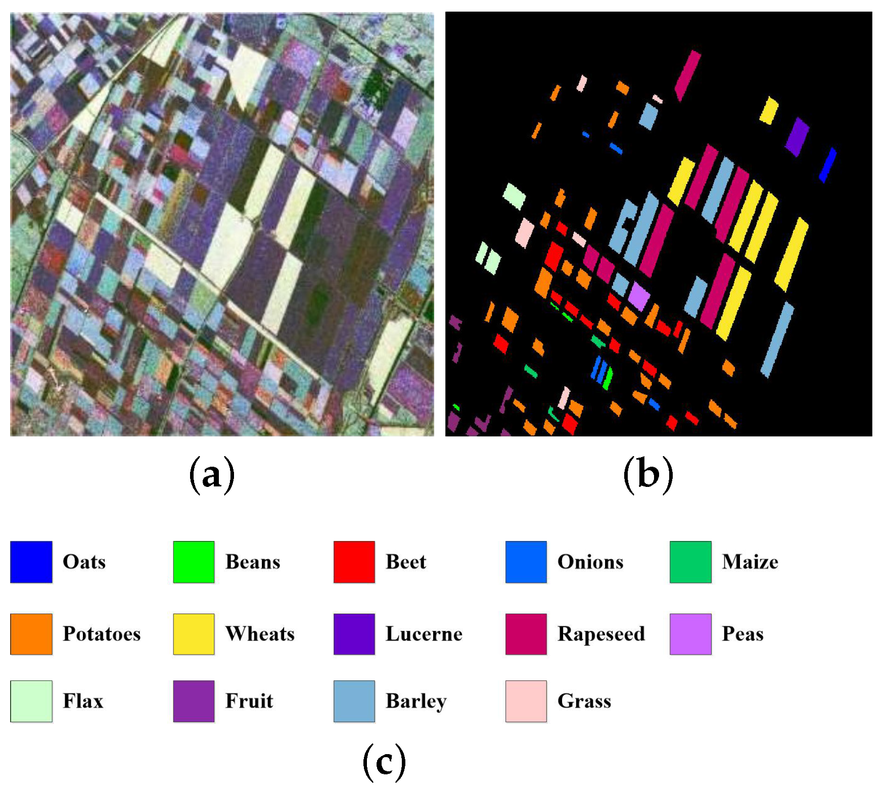
3. PolSAR Data Processing

For PolSAR images, the complex scattering matrix $\mathcal{S}$ is usually used to capture the scattering characteristics of a single target through HH, HV, VH, and VV polarization channels, which can be expressed as

$$\mathcal{S}=\left[\begin{array}{cc}{\mathcal{S}}_{\mathrm{HH}}& {\mathcal{S}}_{\mathrm{HV}}\\ {\mathcal{S}}_{\mathrm{VH}}& {\mathcal{S}}_{\mathrm{VV}}\end{array}\right],$$

where “H” and “V” denote the orthogonal horizontal/vertical polarization directions, respectively, ${\mathcal{S}}_{\mathrm{HV}}$ is the complex scattering coefficient of horizontal transmitting and vertical receiving polarization, and the other coefficients are similarly defined. In the case of reciprocal backscattering, ${\mathcal{S}}_{\mathrm{HV}}={\mathcal{S}}_{\mathrm{VH}}$, and $\mathcal{S}$ based on the Pauli basis [47] can be represented by a complex scattering vector ${\mathit{k}}_{3\mathrm{P}}$,

$${\mathit{k}}_{3\mathrm{P}}=\frac{1}{\sqrt{2}}{[{\mathcal{S}}_{\mathrm{HH}}+{\mathcal{S}}_{\mathrm{VV}},{\mathcal{S}}_{\mathrm{HH}}-{\mathcal{S}}_{\mathrm{VV}},2{\mathcal{S}}_{\mathrm{HV}}]}^T,$$

where subscript T denotes the matrix transpose.

Thus, the coherency matrix $\mathbf{T}$ of PolSAR data can be obtained as follows:

$$\mathbf{T}={\mathit{k}}_{3\mathrm{P}}{\mathit{k}}_{3\mathrm{P}}^H=\left[\begin{array}{ccc}{T}_{11}& T_{12}& T_{13}\\ T_{12}^{\ast }& T_{22}& T_{23}\\ T_{13}^{\ast }& T_{23}^{\ast }& T_{33}\end{array}\right],$$

where subscript H and ∗ denote the conjugate transpose and conjugate operation, respectively. Therefore, the upper triangular elements ($T_{11}$, $T_{12}$, $T_{13}$, $T_{22}$, $T_{23}$, $T_{33}$) of the coherency matrix $\mathbf{T}$ are used as the input dataset of ACV-CWNN-MRF, and $R=6$.

After the preprocessing of the input datasets, such as expansion operation, data augmentation (DA), and batch normalization (BN), we can obtain a higher classification accuracy for PolSAR images.

4. Results

In order to verify the effectiveness of the proposed ACV-CWNN-MRF approach, a series of experiments on three real PolSAR datasets are analyzed and compared with some state-of-the-art deep learning-based methods in the following experiments. The overall accuracy (OA), average accuracy (AA), Kappa coefficient ($\kappa$), and the confusion matrix are used to evaluate the performance on the proposed ACV-CWNN-MRF method. Details about these three benchmark PolSAR datasets are described as follows. We randomly select some samples as the training dataset and the remaining samples as the testing dataset.

(1) Flevoland Dataset: This dataset was acquired by the NASA/JPL AIRSAR platform over an agriculture area of the Netherlands on August 1989, and is a subset of an L-band, full PolSAR image with a range resolution of $6.6$ m and an azimuth resolution of $12.1$ m. There are, in total, 15 identified categories, including stem beans, beet, barley, peas, potatoes, three types of wheat, forest, bare soil, lucerne, grasses, water, rapeseed, and buildings. The PauliRGB image of the Flevoland dataset is shown in Figure 3a, whose size is $750\times 1024$ pixels. A ground-truth map of the 15 categories and a corresponding color legend of the ground-truth map are shown in Figure 3b,c, respectively.

(2) Benchmark Dataset: A Benchmark PolSAR dataset of another L-band full PolSAR image was acquired over the Flevoland area in 1991, and is widely used for PolSAR image classification research. The size of the PolSAR image is $1020\times 1024$ pixels. There are, in total, 14 identified categories, including oats, potatoes, flax, beans, wheats, fruit, beet, lucerne, barley, onions, rapeseed, grass, maize, and peas. The PauliRGB image of the Flevoland dataset, a ground-truth map of the 14 categories, and a corresponding color legend of the ground-truth map are shown in Figure 4a–c, respectively.

(3) CONVAIR Ice Dataset: The third dataset comprises multilook CONVAIR C-band full PolSAR data obtained over an ice area in Canada in 2001. The original PolSAR image has dimensions of $544\times 5238$ pixels with a spatial resolution of 4 m × 0.43 m. This Pauli RGB image with $544\times 523$ pixels in Figure 5a was produced by using 10x Azimuth MultiLooking during the CONVAIR data extraction and conversion process. There are, in total, five identified categories, including leads, ThI (thin ice, new forming ice), rough FYI (rough First-Year Ice), ridged FYI (ridged First-Year Ice), FYI-1 (floes, far range), and FYI-2 (floes, near range). A ground-truth map of the five categories and a corresponding color legend of the ground-truth map are shown in Figure 5b,c, respectively.

4.1. Parameter Setting

In this subsection, we conduct an experiment to evaluate the effectiveness of our proposed ACV-CWNN-MRF method for PolSAR image classification incorporating four key strategies: (1) batch normalization (BN); (2) data augmentation (DA); (3) active learning (AL); (4) MRF optimization. In this experiment, the baseline method is CV-CWNN. To discuss the effectiveness of these strategies, we establish four comparison methods which gradually add each of the other techniques.

(1)

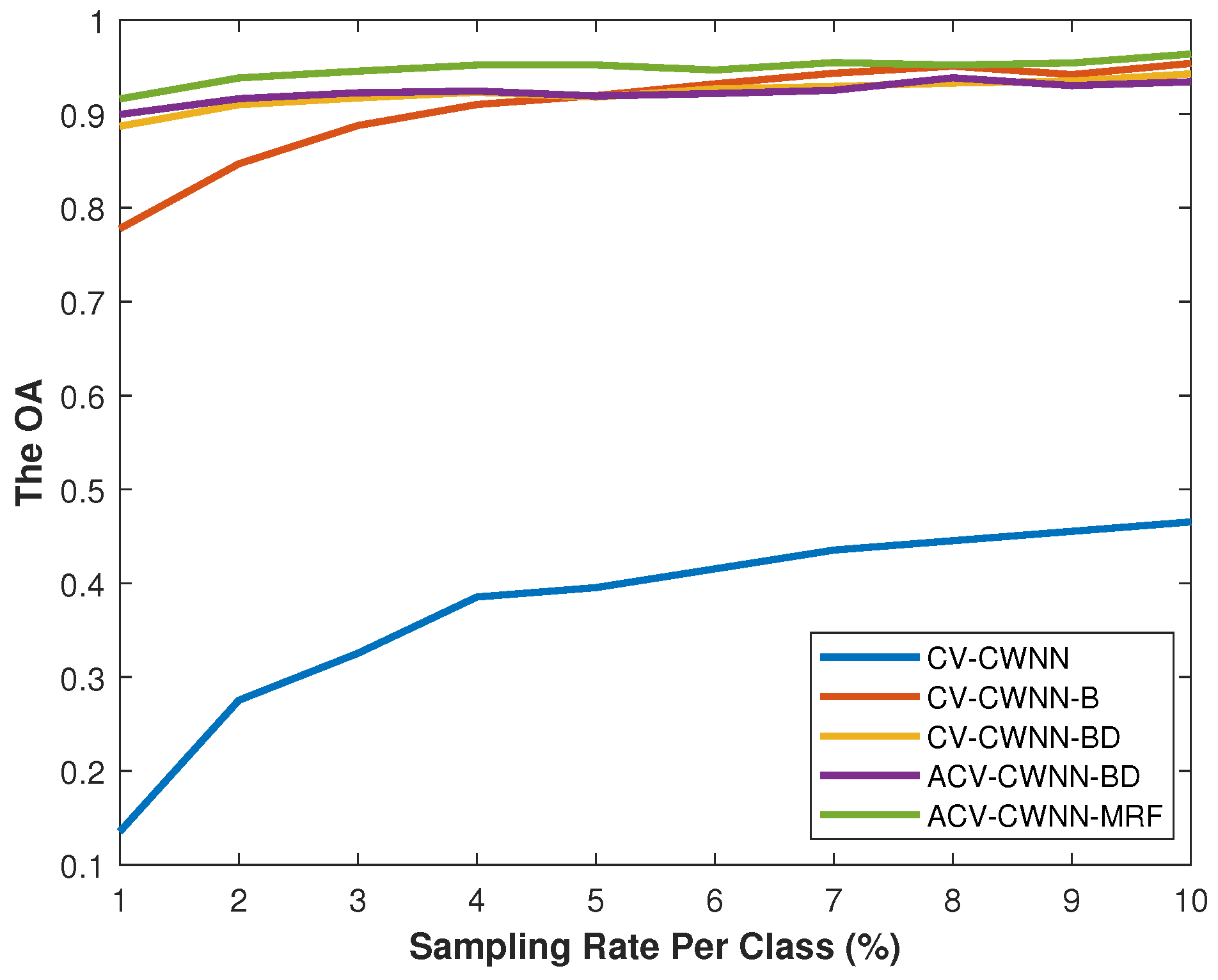
CV-CWNN: The method that is introduced in Section 2.1.

(2)

CV-CWNN + BN (CV-CWNN-B): A method that combines the CV-CWNN method and BN strategy.

(3)

CV-CWNN + BN + DA (CV-CWNN-BD): A method that incorporates the CV-CWNN-B method with the DA strategy.

(4)

CV-CWNN + BN + DA + AL (ACV-CWNN-BD): A method that integrates the AL strategy with the CV-CWNN-BD method.

(5)

CV-CWNN + BN + DA + AL +MRF (ACV-CWNN-MRF): A method that integrates the MRF optimization strategy with the ACV-CWNN-BD method.

We take the Flevoland dataset to construct the experiment, and the relevant experimental parameters for the CV-CWNN-based methods are set as follows. The learning rate $\eta$ is set at 0.6. The batchsize is empirically set as 128. For all the methods, we conduct two rounds for training in the experiments and randomly select different sample rate of available labeled samples for training. For non-AL based methods, including CV-CWNN, CV-CWNN-B, and CV-CWNN-BD, each round contains 40 training epochs until the training model converges. For AL based methods, including ACV-CWNN-BD and ACV-CWNN-MRF, the first round contains 15 training epochs, while the second round contains 20 training epochs. Specifically, for the first round, we randomly choose 500 labeled samples as the training dataset and the remaining samples as the testing dataset. For the second round, we randomly add 50 samples into the training set for the non-AL based methods and actively select 50 samples to enlarge the training set for the AL based methods. We compute The average OA and the standard derivation of CV-CWNN based methods by averaging 5 independent runs. The experimental results are recorded in

Table 1. The average OA and the standard derivation (%) of CV-CWNN based methods with different strategies for PolSAR classification.

Method	CV-CWNN	CV-CWNN-B	CV-CWNN-BD	ACV-CWNN-BD	ACV-CWNN-MRF
1st round, 500 samples	11.52 (2.86)	17.16 (1.51)	46.29 (2.12)	60.74 (2.47)	61.66 (1.51)
2st round, 550 samples	12.26 (1.80)	28.13 (2.91)	68.85 (1.92)	70.14 (2.92)	72.33 (2.14)

.

From Table 1, we can observe by column that each method has better performance as the round carries out, which is due to add some samples into the training dataset after the first round. From the results by row, we observe that the different strategy can improve classification and recognition performance. Specifically, CV-CWNN-B can first obtain a classification OA of up to $10\%$ improvement compared with CV-CWNN. Second, DA strategy can achieve an increase of approximately $35\%$ OA by comparing CV-CWNN-BD and CV-CWNN-B. Next, compared with CV-CWNN-B, ACV-CWNN-BD with AL strategy increase OA by about $8\%$. Finally, MRF strategy can further obtain about $1.5\%$ improvement of classification OA. Therefore, it demonstrates that each different strategy used in the CV-CWNN based methods can improve the overall classification performance.

Second, in order to evaluate the performance of the CV-CWNN based methods and investigate an optimal sampling rate, we carry out the contrasting experiments on the overall accuracy (OA) versus different sampling rate per class. As can be seen from Figure 6, when the sampling rate is $1\%$, the OA of ACV-CWNN-MRF is approximately $91.61\%$, and as the sampling rate approaches $4\%$, the accuracy quickly rises to $95\%$. It follows that for the Flevoland data set, a $5\%$ sample rate is sufficient for ACV-CWNN-MRF. Indeed, it is observable from Figure 6 that as the number of training samples increases, the accuracy of all CV-CWNN based classification methods improves. Additionally, it is evident that each technique is capable of enhancing the classification performance of the CV-CWNN based model to a certain extent.

4.2. Effectiveness Verification

We present our proposed method’s performance and analysis using the Benchmark Dataset. According to the discussions aforementioned, for training, we randomly select $5\%$ of the available labeled samples each class. For AL based methods, the first round contains 15 training epochs, while the second round contains 20 training epochs. For the second round, we randomly add 50 samples into the training set for the non-AL based methods and actively select 50 samples to enlarge the training set for the AL based methods. The size of a local patch is 12. The classification maps achieved by the CV-CWNN based methods are shown in Figure 7, and the classification accuracies are reported in

Table 2. Classification accuracies (%) for the Benchmark dataset with 15 training epochs the first round and 20 training epochs the second round by different methods.

Class	CV-CWNN	CV-CWNN-B	CV-CWNN-BD	ACV-CWNN-BD	ACV-CWNN-MRF
1	0	99.78	99.54	99.63	99.80
2	0	90.83	91.27	91.54	95.39
3	0	50.34	93.74	92.88	96.67
4	0	99.09	98.58	96.94	97.70
5	99.94	99.65	99.76	99.94	99.95
6	0	0.15	42.34	46.47	57.50
7	0	99.82	99.71	99.67	99.78
8	0	0	49.71	80.90	88.60
9	0	92.73	99.07	96.87	98.73
10	0	0	94.05	95.40	98.19
11	0	96.21	95.37	95.42	97.28
12	99.39	99.84	99.63	99.78	99.70
13	0	71.49	88.03	82.24	87.32
14	0	93.69	93.33	95.97	96.40
AA	14.24	70.97	88.87	90.89	93.79
OA	38.85	94.37	97.25	97.36	98.14
$\kappa$	24.19	93.35	96.75	96.89	97.80

. It is evident from Table 2 that, when compared to all other approaches, the proposed ACV-CWNN-MRF method performs the best in terms of AA and OA metrics. Comparing the CAs of all the CV-CWNN based methods, it can be seen that the suggested method has the best classification accuracy in the majority of the classes. Furthermore, Figure 7 shows that the proposed ACV-CWNN-MRF method can produce smoother and more accurate classification maps.

5. Discussion

In this section, we compare the ACV-CWNN-MRF method with other some state-of-the-art PolSAR classification methods on CONVAIR Ice dataset with the speckle noise. These compared methods include real-valued CNN (RV-CNN) [14], real-valued CNN-MRF (RV-CNN-MRF) [48], complex-valued CNN (CV-CNN) [17], and real-valued CNN-AL-MRF (RV-CNN-AL-MRF) [25]. The experimental settings for the CONVAIR Ice dataset are as follows. For all methods, there are 238 training samples altogether since we choose $5\%$ of the CONVAIR Ice dataset at random from each class to use as the training set. The learning rate $\eta$ is set as $0.8$. The batch size is empirically set at 100. For RV-CNN, RV-CNN-MRF, and CV-CNN, each round contains 50 epochs, which do not employ the AL strategy, while for RV-CNN-AL-MRF and ACV-CWNN-MRF, the first round contains 25 epochs and the second round contains 50 epochs. For the second round, we actively select 50 samples to enlarge the training set for the AL-based methods.

The speckle noise in the PolSAR image of the HH, HV, VH, and VV polarization channels is modeled as a multiplicative form, which can be expressed as $\tilde{f}=f+\gamma \times f$, where $f={\mathcal{S}}_{\mathrm{HH}},{\mathcal{S}}_{\mathrm{HV}},{\mathcal{S}}_{\mathrm{VH}}$, and ${\mathcal{S}}_{\mathrm{VV}}$, and $\gamma$ is white Gaussian noise. The original multiplicative noise of the PolSAR speckling model can be converted to an additive case by the logarithmic operation $log\left(\tilde{f}\right)=log\left(f\right)+log(\gamma +1)$. Therefore, the log-transformed speckle model of PolSAR images can also be regarded as an additive white Gaussian noise model with a mean of 0 and variance $\sigma$ for mathematical tractability [49]. We consider the range of the level $\gamma$ of speckle noise as $\gamma \in [0.02,0.18]$, and the local patch size as $12\times 12$, so as to train the compared model and the proposed model for PolSAR classification.

Finally, the overall accuracies (OAs), the average accuracies (AAs), and the Kappa coefficients ($\kappa$) for all considered methods with different noise levels of speckles are reported in Figure 8. Visually, Figure 8 shows that as the level $\gamma$ of speckle noise increases, the PolSAR image classification performance for all considered methods will decrease. Moreover, when the noise level exceeds $0.08$, the classification performance drops sharply. However, it can be also easily observed that in the presence of PolSAR speckle noise, our ACV-CWNN-MRF method achieves the best performance in OA, AA, and $\kappa$ on the CONVAIR Ice dataset compared with the other four methods. The superior classification performance of our ACV-CWNN-MRF method can be explained by exploiting the CWNN and MRF strategy simultaneously, where the complex-valued wavelet pooling layer of CWNN can not only remove some PolSAR speckle noise, but it can also maintain the structures of the feature maps in accordance with the specified rules. Additionally, classification maps of the CONVAIR Ice dataset with noise levels of $\gamma =0.02$ and $\gamma =0.16$ using different methods are presented in Figure 9 and Figure 10, respectively. It can be visually seen from Figure 9 and Figure 10 that our ACV-CWNN-MRF method for the despeckled PolSAR classification achieves a smoother classification map than RV-CNN, RV-CNN-MRF, RF-CNN-AL-MRF, and CV-CNN. According to the aforementioned discussions, our ACV-CWNN-MRF method can suppress the influence of speckle noise and obtain more accurate, smooth, and coherent classification performance.

6. Conclusions

In this paper, we have proposed a novel PolSAR image classification method based on an active complex-valued convolutional-wavelet neural network framework by incorporating dual-tree complex wavelet transform and Markov random field. Our proposed ACV-CWNN-MRF method has the following advantages. Firstly, we introduce a DT-CWT-constrained pooling layer into CV-CNN-based PolSAR classification to suppress speckle noise in a PolSAR image and maintain the SAR image structure information. Secondly, we combine the AL and MRF strategies into CV-CWNN to obtain the most informative unlabeled training samples and achieve the local correlation of neighboring pixels. Finally, experiments on three benchmark PolSAR datasets show that our proposed ACV-CWNN-MRF method can outperform some other state-of-the-art deep learning-based PolSAR image classification methods. We conclude that our fine-tuned ACV-CWNN-MRF method is an effective alternative method for PolSAR classification. We will continue to study how to better perform PolSAR classification on our own datasets in our future work.

References

1. Cloude, S. Polarisation: Applications in Remote Sensing; OUP Oxford: Oxford, UK, 2009. [Google Scholar]
2. Lee, J.S.; Pottier, E. Polarimetric Radar Imaging: From Basics to Applications; CRC Press: Boca Raton, FL, USA, 2017. [Google Scholar]
3. Hänsch, R.; Hellwich, O. Skipping the real world: Classification of PolSAR images without explicit feature extraction. ISPRS J. Photogramm. Remote Sens. 2018, 140, 122–132. [Google Scholar] [CrossRef]
4. Durieux, L.; Lagabrielle, E.; Nelson, A. A method for monitoring building construction in urban sprawl areas using object-based analysis of Spot 5 images and existing GIS data. ISPRS J. Photogramm. Remote Sens. 2008, 63, 399–408. [Google Scholar] [CrossRef]
5. Zhong, P.; Wang, R. A multiple conditional random fields ensemble model for urban area detection in remote sensing optical images. IEEE Trans. Geosci. Remote Sens. 2007, 45, 3978–3988. [Google Scholar] [CrossRef]
6. Besic, N.; Vasile, G.; Chanussot, J.; Stankovic, S. Polarimetric incoherent target decomposition by means of independent component analysis. IEEE Trans. Geosci. Remote Sens. 2014, 53, 1236–1247. [Google Scholar] [CrossRef]
7. Doulgeris, A.P.; Anfinsen, S.N.; Eltoft, T. Classification with a non-Gaussian model for PolSAR data. IEEE Trans. Geosci. Remote Sens. 2008, 46, 2999–3009. [Google Scholar] [CrossRef]
8. Kong, J.; Swartz, A.; Yueh, H.; Novak, L.; Shin, R. Identification of terrain cover using the optimum polarimetric classifier. J. Electromagn. Waves Appl. 1988, 2, 171–194. [Google Scholar]
9. Tao, M.; Zhou, F.; Liu, Y.; Zhang, Z. Tensorial independent component analysis-based feature extraction for polarimetric SAR data classification. IEEE Trans. Geosci. Remote Sens. 2014, 53, 2481–2495. [Google Scholar] [CrossRef]
10. Lardeux, C.; Frison, P.L.; Tison, C.; Souyris, J.C.; Stoll, B.; Fruneau, B.; Rudant, J.P. Support vector machine for multifrequency SAR polarimetric data classification. IEEE Trans. Geosci. Remote Sens. 2009, 47, 4143–4152. [Google Scholar] [CrossRef]
11. Ersahin, K.; Cumming, I.G.; Ward, R.K. Segmentation and classification of polarimetric SAR data using spectral graph partitioning. IEEE Trans. Geosci. Remote Sens. 2009, 48, 164–174. [Google Scholar] [CrossRef]
12. Bi, H.; Sun, J.; Xu, Z. Unsupervised PolSAR image classification using discriminative clustering. IEEE Trans. Geosci. Remote Sens. 2017, 55, 3531–3544. [Google Scholar] [CrossRef]
13. Antropov, O.; Rauste, Y.; Astola, H.; Praks, J.; Häme, T.; Hallikainen, M.T. Land cover and soil type mapping from spaceborne PolSAR data at L-band with probabilistic neural network. IEEE Trans. Geosci. Remote Sens. 2013, 52, 5256–5270. [Google Scholar] [CrossRef]
14. Zhou, Y.; Wang, H.; Xu, F.; Jin, Y.Q. Polarimetric SAR image classification using deep convolutional neural networks. IEEE Geosci. Remote Sens. Lett. 2016, 13, 1935–1939. [Google Scholar] [CrossRef]
15. Liu, F.; Jiao, L.; Hou, B.; Yang, S. POL-SAR image classification based on Wishart DBN and local spatial information. IEEE Trans. Geosci. Remote Sens. 2016, 54, 3292–3308. [Google Scholar] [CrossRef]
16. Jiao, L.; Liu, F. Wishart deep stacking network for fast POLSAR image classification. IEEE Trans. Image Process. 2016, 25, 3273–3286. [Google Scholar] [CrossRef] [PubMed]
17. Zhang, Z.; Wang, H.; Xu, F.; Jin, Y.Q. Complex-valued convolutional neural network and its application in polarimetric SAR image classification. IEEE Trans. Geosci. Remote Sens. 2017, 55, 7177–7188. [Google Scholar] [CrossRef]
18. Bi, H.; Sun, J.; Xu, Z. A graph-based semisupervised deep learning model for PolSAR image classification. IEEE Trans. Geosci. Remote Sens. 2018, 57, 2116–2132. [Google Scholar] [CrossRef]
19. Tuia, D.; Ratle, F.; Pacifici, F.; Kanevski, M.F.; Emery, W.J. Active learning methods for remote sensing image classification. IEEE Trans. Geosci. Remote Sens. 2009, 47, 2218–2232. [Google Scholar] [CrossRef]
20. Tuia, D.; Volpi, M.; Copa, L.; Kanevski, M.; Munoz-Mari, J. A survey of active learning algorithms for supervised remote sensing image classification. IEEE J. Sel. Top. Signal Process. 2011, 5, 606–617. [Google Scholar] [CrossRef]
21. Samat, A.; Gamba, P.; Du, P.; Luo, J. Active extreme learning machines for quad-polarimetric SAR imagery classification. Int. J. Appl. Earth Obs. Geoinf. 2015, 35, 305–319. [Google Scholar] [CrossRef]
22. Liu, W.; Yang, J.; Li, P.; Han, Y.; Zhao, J.; Shi, H. A novel object-based supervised classification method with active learning and random forest for PolSAR imagery. Remote Sens. 2018, 10, 1092. [Google Scholar] [CrossRef]
23. Bi, H.; Xu, F.; Wei, Z.; Xue, Y.; Xu, Z. An active deep learning approach for minimally supervised PolSAR image classification. IEEE Trans. Geosci. Remote Sens. 2019, 57, 9378–9395. [Google Scholar] [CrossRef]
24. Li, J.; Bioucas-Dias, J.M.; Plaza, A. Spectral–spatial classification of hyperspectral data using loopy belief propagation and active learning. IEEE Trans. Geosci. Remote Sens. 2012, 51, 844–856. [Google Scholar] [CrossRef]
25. Cao, X.; Yao, J.; Xu, Z.; Meng, D. Hyperspectral image classification with convolutional neural network and active learning. IEEE Trans. Geosci. Remote Sens. 2020, 58, 4604–4616. [Google Scholar] [CrossRef]
26. De Silva, D.; Fernando, S.; Piyatilake, I.; Karunarathne, A. Wavelet based edge feature enhancement for convolutional neural networks. In Proceedings of the Eleventh International Conference on Machine Vision (ICMV 2018), Munich, Germany, 1–3 November 2018; International Society for Optics and Photonics: Bellingham, WA, USA, 2019; Volume 11041, p. 110412R. [Google Scholar]
27. Liu, P.; Zhang, H.; Lian, W.; Zuo, W. Multi-level wavelet convolutional neural networks. IEEE Access 2019, 7, 74973–74985. [Google Scholar] [CrossRef]
28. Sahito, F.; Zhiwen, P.; Ahmed, J.; Memon, R.A. Wavelet-integrated deep networks for single image super-resolution. Electronics 2019, 8, 553. [Google Scholar] [CrossRef]
29. Guberman, N. On complex valued convolutional neural networks. arXiv 2016, arXiv:1602.09046. [Google Scholar]
30. Tygert, M.; Bruna, J.; Chintala, S.; LeCun, Y.; Piantino, S.; Szlam, A. A mathematical motivation for complex-valued convolutional networks. Neural Comput. 2016, 28, 815–825. [Google Scholar] [CrossRef]
31. Trabelsi, C.; Bilaniuk, O.; Zhang, Y.; Serdyuk, D.; Subramanian, S.; Santos, J.; Mehri, S.; Rostamzadeh, N.; Bengio, Y.; Pal, C. Deep Complex Networks. arXiv 2018, arXiv:1705.09792. [Google Scholar]
32. Benvenuto, N.; Piazza, F. On the complex backpropagation algorithm. IEEE Trans. Signal Process. 1992, 40, 967–969. [Google Scholar] [CrossRef]
33. Lau, M.M.; Lim, K.H.; Gopalai, A.A. Malaysia traffic sign recognition with convolutional neural network. In Proceedings of the 2015 IEEE International Conference on Digital Signal Processing (DSP), Singapore, 21–24 July 2015; IEEE: Piscataway, NJ, USA, 2015; pp. 1006–1010. [Google Scholar]
34. Kingsbury, N. Complex wavelets for shift invariant analysis and filtering of signals. Appl. Comput. Harmon. Anal. 2001, 10, 234–253. [Google Scholar] [CrossRef]
35. Baraniuk, R.; Kingsbury, N.; Selesnick, I. The dual-tree complex wavelet transform-a coherent framework for multiscale signal and image processing. IEEE Signal Process. Mag. 2005, 22, 123–151. [Google Scholar]
36. Kingsbury, N. Image processing with complex wavelets. Philos. Trans. R. Soc. Lond. Ser. A Math. Phys. Eng. Sci. 1999, 357, 2543–2560. [Google Scholar]
37. Rumelhart, D.E.; Hinton, G.E.; Williams, R.J. Learning representations by back-propagating errors. Nature 1986, 323, 533–536. [Google Scholar]
38. Bengio, Y. Practical recommendations for gradient-based training of deep architectures. In Neural Networks: Tricks of the Trade; Springer: Berlin/Heidelberg, Germany, 2012; pp. 437–478. [Google Scholar]
39. MacKay, D.J. Information-based objective functions for active data selection. Neural Comput. 1992, 4, 590–604. [Google Scholar]
40. Luo, T.; Kramer, K.; Goldgof, D.B.; Hall, L.O.; Samson, S.; Remsen, A.; Hopkins, T.; Cohn, D. Active learning to recognize multiple types of plankton. J. Mach. Learn. Res. 2005, 6, 589–613. [Google Scholar]
41. Settles, B. Active learning. Synth. Lect. Artif. Intell. Mach. Learn. 2012, 6, 1–114. [Google Scholar]
42. Joshi, A.J.; Porikli, F.; Papanikolopoulos, N. Multi-class active learning for image classification. In Proceedings of the 2009 IEEE Conference on Computer Vision and Pattern Recognition, Miami, FL, USA, 20–25 June 2009; IEEE: Piscataway, NJ, USA, 2009; pp. 2372–2379. [Google Scholar]
43. Farag, A.A.; Mohamed, R.M.; El-Baz, A. A unified framework for map estimation in remote sensing image segmentation. IEEE Trans. Geosci. Remote Sens. 2005, 43, 1617–1634. [Google Scholar]
44. Boykov, Y.; Veksler, O.; Zabih, R. Fast approximate energy minimization via graph cuts. IEEE Trans. Pattern Anal. Mach. Intell. 2001, 23, 1222–1239. [Google Scholar]
45. Kolmogorov, V. Convergent tree-reweighted message passing for energy minimization. In Proceedings of the International Workshop on Artificial Intelligence and Statistics, Bridgetown, Barbados, 6–8 January 2005; pp. 182–189. [Google Scholar]
46. Yedidia, J.S.; Freeman, W.T.; Weiss, Y. Constructing free-energy approximations and generalized belief propagation algorithms. IEEE Trans. Inf. Theory 2005, 51, 2282–2312. [Google Scholar]
47. Cloude, S.R.; Pottier, E. A review of target decomposition theorems in radar polarimetry. IEEE Trans. Geosci. Remote Sens. 1996, 34, 498–518. [Google Scholar]
48. Cao, X.; Zhou, F.; Xu, L.; Meng, D.; Xu, Z.; Paisley, J. Hyperspectral image classification with Markov random fields and a convolutional neural network. IEEE Trans. Image Process. 2018, 27, 2354–2367. [Google Scholar] [CrossRef] [PubMed]
49. Xie, H.; Pierce, L.E.; Ulaby, F.T. Statistical properties of logarithmically transformed speckle. IEEE Trans. Geosci. Remote Sens. 2002, 40, 721–727. [Google Scholar] [CrossRef]
Figure 1. The configuration of ACV-CWNN-MRF architecture for PolSAR image classification.
Remotesensing 16 01094 g001
Figure 2. Flowchart of 2D DTCWT for level j 0 = 1 .
Remotesensing 16 01094 g002
Figure 3. Flevoland dataset. (a) Pauli RGB image of the target scene. (b) Ground-truth map of the 15 categories. (c) Color legend of the ground-truth map.
Remotesensing 16 01094 g003
Figure 4. Benchmark dataset. (a) Pauli RGB image of the target scene. (b) Ground-truth map of the 14 categories. (c) Color legend of the ground-truth map.
Remotesensing 16 01094 g004
Figure 5. CONVAIR Ice dataset. (a) Pauli RGB image of the target scene. (b) Ground-truth map of the 5 categories. (c) Color legend of the ground-truth map.
Remotesensing 16 01094 g005
Figure 6. The overall accuracy (OA) obtained by all CV-CWNN based methods with different numbers of training samples on the Flevoland dataset.
Remotesensing 16 01094 g006
Figure 7. Classification maps for the Benchmark dataset with 15 training epochs the first round and 20 training epochs the second round by different methods. (a,f) CV-CWNN classified map. (b,g) CV-CWNN-B classified map. (c,h) CV-CWNN-BD classified map. (d,i) ACV-CWNN-BD classified map. (e,j) ACV-CWNN-MRF classified map.
Remotesensing 16 01094 g007
Figure 8. The OA, AA, and Kappa coefficient versus the level γ of speckle noise using different classification methods on CONVAIR Ice dataset. (a) OA vs. γ curves. (b) AA vs. γ curves. (c) κ vs. γ curves.
Remotesensing 16 01094 g008
Figure 9. Classification maps of the CONVAIR Ice dataset with noise level γ = 0.02 using different methods. (Top row) Results of the whole map classification. (Bottom row) Result overlaid with the ground-truth map. (a,f) RV-CNN-classified map. (b,g) RV-CNN-MRF-classified map. (c,h) RV-CNN-AL-MRF-classified map. (d,i) CV-CNN-classified map. (e,j) ACV-CWNN-MRF-classified map.
Remotesensing 16 01094 g009
Figure 10. Classification maps of the CONVAIR Ice dataset with noise level γ = 0.16 using different methods. (Top row) Results of the whole map classification. (Bottom row) Result overlaid with the ground-truth map. (a,f) RV-CNN-classified map. (b,g) RV-CNN-MRF-classified map. (c,h) RV-CNN-AL-MRF-classified map. (d,i) CV-CNN-classified map. (e,j) ACV-CWNN-MRF-classified map.
Remotesensing 16 01094 g010